Article

Regression Modeling of Daily PM2.5 Concentrations with a Multilayer Perceptron

1
Faculty of Infrastructure and Environment, Czestochowa University of Technology, 69 Dabrowskiego St., 42-200 Czestochowa, Poland
2
Faculty of Electrical Engineering, Czestochowa University of Technology, 17 Armii Krajowej, 42-200 Czestochowa, Poland
*
Author to whom correspondence should be addressed.
Energies 2024, 17(9), 2202; https://doi.org/10.3390/en17092202
Submission received: 14 March 2024 / Revised: 25 April 2024 / Accepted: 30 April 2024 / Published: 3 May 2024
(This article belongs to the Collection Energy Economics and Policy in Developed Countries)

Abstract

:
Various types of energetic fuel combustion processes emit dangerous pollutants into the air, including aerosol particles, marked as PM10. Routine air quality monitoring includes determining the PM10 concentration as one of the basic measurements. At some air monitoring stations, the PM10 measurement is supplemented by the simultaneous determination of the concentration of PM2.5 as a finer fraction of suspended particles. Since the PM2.5 fraction has a significant share in the PM10 fraction, the concentrations of both types of particles should be strongly correlated, and the concentrations of one of these fractions can be used to model the concentrations of the other fraction. The aim of the study was to assess the error of predicting PM2.5 concentration using PM10 concentration as the main predictor. The analyzed daily concentrations were measured at 11 different monitoring stations in Poland and covered the period 2010–2021. MLP (multilayer perceptron) artificial neural networks were used to approximate the daily PM2.5 concentrations. PM10 concentrations and time variables were tested as predictors in neural networks. Several different prediction errors were taken as measures of modeling quality. Depending on the monitoring station, in models with one PM10 predictor, the RMSE error values were in the range of 2.31–6.86 μg/m3. After taking into account the second predictor D (date), the corresponding RMSE errors were lower and were in the range of 2.06–5.54 μg/m3. Our research aimed to find models that were as simple and universal as possible. In our models, the main predictor is the PM10 concentration; therefore, the only condition to be met is monitoring the measurement of PM10 concentrations. We showed that models trained at other air monitoring stations, so-called foreign models, can be successfully used to approximate PM2.5 concentrations at another station.

1. Introduction

As knowledge about air pollution deepens, new information about the threats resulting from the presence of these pollutants reaches public awareness. Threats concern various aspects of social life. The most obvious and longest historically studied threat is the adverse impact of pollution on human life and health. Research confirms that air pollution also affects animals, plants and other living organisms [1,2,3]. It can cause large losses in animal husbandry and crop yields, therefore causing losses in agriculture [4,5,6]. Pollution also has a direct or indirect adverse impact on other sectors of the economy [7,8,9,10,11].
Basic air pollutants are emitted by natural processes. Anthropogenic emissions, mainly related to energy production, introduce additional amounts of pollutants into the air and cause pollutant concentrations to reach unnaturally high levels [12]. In the case of large anthropogenic emissions and in unfavorable weather, concentrations of toxic pollutants may be so high that they threaten not only health but also the lives of people, animals and other organisms. The first historically documented strong smog episode was recorded on 5–9 December 1952 in London [13]. According to medical statistics, about 4000 people died and about 150,000 were hospitalized. According to the reports, people suffered from respiratory failure and hypoxia, i.e., oxygen deficiency. These were the first documented medical diagnoses of the reasons for death and hospitalization. Until today, it has been recognized that air pollution can cause bronchial and lung diseases [14,15,16], cancer [17,18] and also cardiovascular diseases [19,20,21,22]. Smog also affects the brain and can deepen mental illnesses and neurological ailments [23,24,25,26].
After this tragic event, the first legal regulations forcing the improvement of air quality (including the Clean Air Act) were passed in Great Britain [27]. There was also a need to monitor the air quality. Intensive research in the field of environmental chemistry was initiated to identify pollutants, mechanisms of their formation and threats to the broadly understood natural environment, including humans, animals and plants. The development of pollution detection techniques enabled the construction of automatic air monitoring stations [28,29]. Currently, networks of air monitoring stations operate in almost all developed and emerging countries of the world. This enables continuous monitoring of air quality and warning against smog episodes.
Typical air monitoring stations are equipped with analyzers enabling continuous measurement of the concentrations of basic gaseous air pollutants: O3, SO2, NOx and CO. Sometimes this measurement package is expanded to include other pollutants, e.g., from the group of volatile organic compounds (VOCs). Studies of atmospheric toxicity revealed that particularly dangerous pollutants can be sorbed on the surfaces of aerosols, which are also ubiquitous in atmospheric air. These pollutants include polycyclic aromatic hydrocarbons (PAHs), heavy metals and many others. Therefore, an important challenge for atmospheric monitoring is to measure the concentration of suspended particles and the pollutants they contain. Initially, attention was focused on the dust fraction with particle sizes up to 10 μm, designated as PM10. The measurement of this aerosol fraction is performed at most automatic air monitoring stations, even those that are poorly equipped.
New research is providing more and more information about the relationship between dust particle size and human exposure risk. It turned out that the worst health effects are observed when inhaling particles smaller than 2.5 μm (the dust fraction called PM2.5). Due to their small size, PM2.5 particles can penetrate much deeper into the respiratory system than PM10 particles. Pollutants collected in particles can reach the bronchi and even the alveoli of the lungs, enter the bloodstream and then spread throughout the body [30,31,32]. Currently, it is the concentration of the PM2.5 fraction that is used to calculate mortality rates, such as the number of premature deaths. It is estimated that in Poland, this number is approximately 40,000 people, which constitutes approximately 0.1% of the population [33]. Particulate matter is considered the main cause of premature death in many other countries around the world [34,35].
The development of measurement techniques enables automatic measurement of PM2.5 concentration. However, this measurement is complicated and expensive. It is performed only at selected air monitoring stations. It should be mentioned that the reference measurement method in the case of PM10 or PM2.5 is the gravimetric method, which involves measuring the mass of dust collected on a special filter [36]. This method has its limitations and is usually used over longer averaging periods than gas concentration measurements. Throughout the European Union, including Poland, a 24 h (daily) measurement period has been adopted as the standard for this type of measurement [37]. To sum up, the results of PM2.5 concentration measurements are key to assessing health effects, but appropriate monitoring is performed in only a few measurement stations. There is a need to increase the density of the PM2.5 measurement network. In the long term, this need will probably be met by measurements of PM2.5 concentrations at each air monitoring station. Until this happens, PM2.5 concentrations can be estimated using modeling techniques.
Modeling air pollution concentrations has a long history. These techniques can be used to fill in missing data in air monitoring systems. They are also used to predict concentrations of selected air pollutants. In the past, classical regression or autoregressive methods were used [38,39,40]. Since the 1990s, artificial intelligence techniques have been increasingly used to model air pollution concentrations [41,42,43,44,45,46,47,48,49,50]. The most popular were models that provide prediction without any data from outside of the monitoring system. They are sometimes called autonomous models [48,49]. Very complex neural models, including deep learning methods, are increasingly used to predict air pollution concentrations [51,52,53]. However, these networks require a lot of data, including external data, and therefore their practical applicability is limited.
Neural networks, even networks with a relatively simple structure, turn out to be useful in regression models if predictors are available that are highly correlated with the variable being modeled. If the goal is to model PM2.5 concentrations at a selected air monitoring station, PM10 concentrations measured at the same location are often also available. In Polish conditions, both types of concentrations are always strongly correlated because PM2.5 is a finer fraction within PM10, and its percentage usually significantly exceeds 50% in the mass of PM10 aerosol [54]. Strong statistical dependencies between PM10 and PM2.5 fractions were also found in reports from other countries [55,56]. PM10 concentration can therefore be considered a universal primary predictor in regression models approximating PM2.5 concentration. This concept was tested in neural network models trained to approximate hourly PM2.5 concentrations [54], and promising results were obtained. It turned out that using simple regression MLP models could yield a small PM2.5 prediction error. It is enough to use time variables and PM10 concentration as explanatory variables. Introducing more predictors only slightly improves the accuracy of MLP regression models. In the studies described below, similar modeling was performed to predict 24 h PM2.5 concentrations. The analysis was performed on data from various air monitoring stations in Poland. We took into consideration the stations where the concentrations of both PM10 and PM2.5 were measured over many years. MLP regression neural networks were used for modeling.
The purpose of the analysis was not to create the most accurate predictive models of PM2.5 concentrations. The main goal was to test the concept of possibly simple predictive models that would use data resources available at most air monitoring stations. It was decided that the key predictor would be the concentration of PM10. Since the modeling concerns 24 h (daily) concentrations, the supporting predictor was a time variable providing information about the time of year. Therefore, the analysis was limited to testing only the two variables mentioned above as predictors. An additional goal was to test the universality of the obtained models. For this purpose, simulations were performed to check whether a neural network trained at one of the stations could be used to predict daily PM2.5 concentrations at other air monitoring stations.

2. Materials and Methods

2.1. Air Monitoring Sites

We took to the examination data from 11 automatic air monitoring stations situated in Poland in the following sites: Jaslo, Katowice, Koscierzyna, Krakow, Lodz, Lublin, Olsztyn, Osieczow, Puszcza Borecka, Zielona Gora and Zielonka. Measurement data cover a period from 2010 to 2021. Monitoring stations were selected to meet two conditions:
  • Their location was diverse enough to cover various regions of Poland;
  • Daily concentrations of both PM10 and PM2.5 fractions were simultaneously measured at each station for at least several years.
The location of the station is shown in Figure 1, where the borders of the administrative division of Poland are marked. All the monitoring stations are operated by the Chief Inspectorate of Environmental Protection in Poland. Table 1 contains background information about the location of individual stations, including addresses, international codes, geographical coordinates, station types and types of monitored area.

2.2. Air Monitoring Data

The 24 h PM10 and PM2.5 concentration values recorded in 2010–2021 were used for the study. The data were provided by the Chief Inspectorate of Environmental Protection in Poland. The provided air monitoring data were validated and officially approved.
The concentration of PM10 and PM2.5 was measured using the gravimetric method [35]. The PM concentrations were calculated on the basis of differences in filter masses before and after daily exposure, which involved passing a specific volume of dust-contaminated air through the filters. The filters were replaced automatically every 24 h. PM concentrations are given in μg/m3.
The following symbols were used to describe the data used:
  • PM10—daily averaged concentration of particles up to 10 μm in size.
  • PM2.5—daily averaged concentration of particles up to 2.5 μm in size.
  • D—date in the numerical form.

2.3. Temporal Variable’s Transformation

The numerical form of the date (D) was prepared in such a way that each date was replaced with a value from the range 0 ÷ 1. For January 1 (the first day of the year), the value was set to 1, and for July 2 (the middle day of the year), the value was set to 0. During the first half of the year, the numerical value of the date decreases linearly from 1 to 0. During the second half of the year, the numerical value of the date increases linearly from 0 to almost 1.
The purpose of transforming the date into such a cyclic numerical form was to assign the same values to similar days in different years. The transformation also made it possible to maintain continuity when changing the year: 31 December and 1 January of the following year have almost identical values.

2.4. Data Preparation

Not all the air monitoring stations carried out measurements for the entire 12 years. Even if measurements were performed, their completeness was sometimes unsatisfactory. Therefore, only the annual series of measurements whose completenesses exceeded 80% were taken into account for the analysis. At lower completeness, the entire annual measurement series was removed from the analyzed set. The aim of this procedure was to ensure that the analyzed cases covered all seasons of a calendar year as evenly as possible. Cases without PM measurements were also removed from the set of analyzed data. Only those cases (days) for which both PM10 and PM2.5 concentration values were known were left to train the network. As for the choice of the station, the principle was adopted that measurements of PM10 and PM2.5 concentrations should be carried out for a minimum of 5 consecutive years. The processed data, prepared for the analysis in this way, have been attached as a Supplemental File.
Table 2 shows the completeness of the data series for individual air monitoring stations, after removing cases with missing data and after removing annual time series with completeness below 80%. Due to the fact that only complete cases were retained, the completeness of data for both PM10 and PM2.5 pollutants was the same.
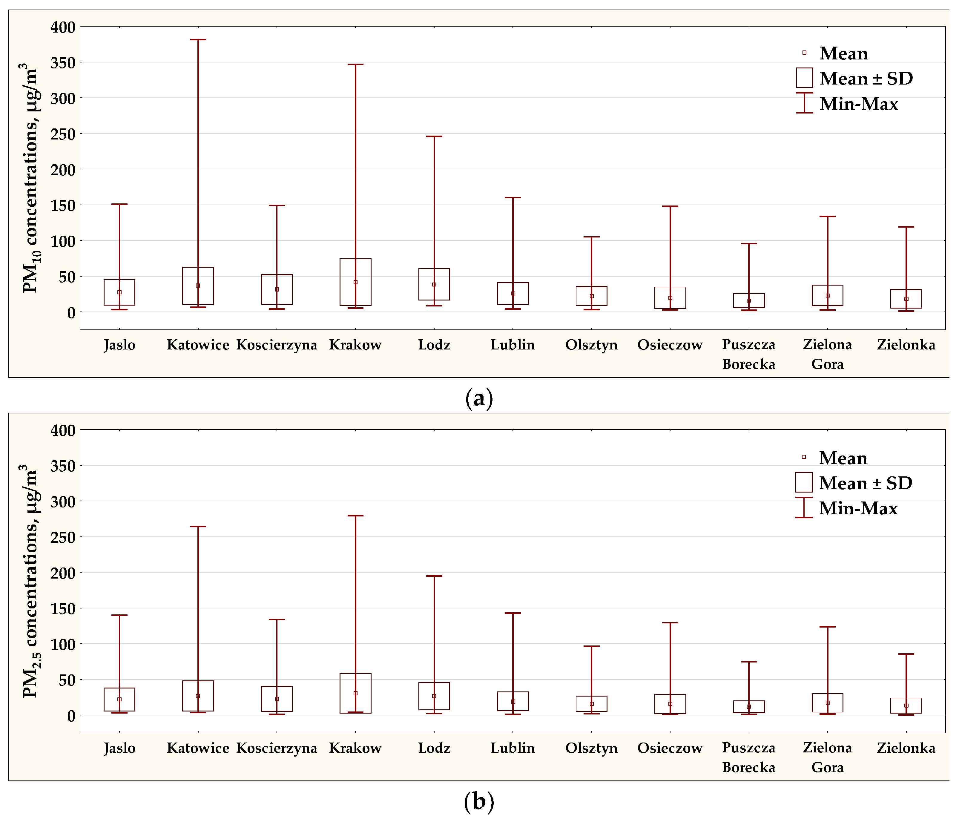
Figure 2 presents a statistical description of the set of daily PM10 and PM2.5 concentrations, measured at considered air monitoring stations, calculated only for complete cases. Among the selected stations, the highest average and maximum concentrations of suspended dust occurred at measuring stations located in large urban agglomerations, i.e., in Katowice, Krakow and Lodz. The lowest values were at air monitoring stations mainly located in rural areas, i.e., Puszcza Borecka, Zielonka, Osieczow and Olsztyn.

2.5. Regression Models

For modeling, the Statistica version 13.3 program was used, together with the SANN (Statistica Artificial Neural Networks) extension subprogram, enabling the creation of neural networks [58]. A separate data set was prepared for each station. The modeling was performed separately for each of the 11 air monitoring stations. The multilayer perceptron (MLP) was adopted in the generated models. It was assumed that all models have the same architecture. All perceptrons have a single hidden layer of 10 neurons. Before training a neural network, a data set was randomly divided into three subsets: a training subset (50% of cases), a testing subset (25% of cases) and a validation subset (25% of cases). The number of all cases in the sets from various air monitoring stations is given in Table 2. The BFGS (Broyden–Fletcher–Goldfarb–Shanno) algorithm was used in the network training process. This algorithm is intended for numerical optimization [59]. The mathematical basis of the algorithm was developed by the above-mentioned mathematicians in 1970 [60,61,62,63].
For all networks, the learning process was stopped after 300 epochs. A logistic activation function was assumed in the hidden neurons and a linear activation function in the output neurons. The network was initialized randomly using the Gaussian method. The initial weights followed a normal distribution with zero mean and unit variance. The sum of squares (SOS) was used as the error function in the network training process. The SOS is the sum of the squares of the differences between the predicted and observed concentration values. For each air monitoring station, the prediction was repeated 5 times, each time with different random assignment of cases to subsets and with different randomly chosen initial weights. The most precise of the 5 generated models was selected for each station, and the results of these most accurate models are presented in the Results section. The accuracy of the models was assessed by calculating 5 different error measures, MAE, RMSE, MARE, R2 and d. The mentioned error measures were described in the next subsection. The networks generated for the same monitoring stations differed slightly in the modeling errors. They had identical neuronal structures but differed in the weights and degrees of activation of individual neurons in the hidden layer. Statistica Neural Networks automatically scales input and output variables using a linear transformation to the interval [0, 1].
For each monitoring station, regression models were created whose output variable was the daily concentration of PM2.5, while the input variables were introduced in one of the three variants:
  • Variant I—D—(MLP 1-10-1, Figure 3a);
  • Variant II—PM10—(MLP 1-10-1, Figure 3b);
  • Variant III—D and PM10—(MLP 2-10-1, Figure 3c).
Figure 3 shows the MLP architectures for these different variants.
In addition to the perceptron models, simpler models were also created to compare accuracy. A linear regression model (LIN) and a naive mean model (MEAN) were generated. In the latter, the average value of PM2.5 concentration was assumed for each station, calculated separately for each station from historical measurements.

2.6. Assessment of the Prediction Accuracy

To assess the accuracy of the obtained MLP artificial neural network models, the following error values were used: MAE (mean absolute error), RMSE (root mean squared error), MARE (mean absolute relative error), R2 (coefficient of determination) and d (Willmott index of agreement). Index d is a special formula dedicated to air quality modeling [64]. These values were calculated by comparing real 24 h PM2.5 concentration values with predicted values. The formulas for calculating the listed errors are given below in Equations (1)–(5).
MAE—Mean Absolute Error
M A E = 1 n i = 1 n x i y i
RMSE—Root Mean Squared Error
R M S E = i = 1 n x i y i 2 n
MARE—Mean Absolute Relative Error
M A R E = 1 n i = 1 n x i y i x i
R2—Coefficient of Determination
R 2 = i = 1 n y i x ¯ 2 i = 1 n x i x ¯ 2
d—Willmott Index of Agreement
d = 1 i = 1 n y i x i 2 i = 1 n y i x ¯ + x i x ¯ 2
where:
n—number of cases;
y—predicted concentrations;
x—real concentrations;
x ¯ —arithmetic average of real concentrations;
i—the case number.

2.7. Verification of Models

Approach 1
In order to check whether it is possible to predict PM2.5 concentrations in a later measurement period using neural networks trained on historical data, a trial modeling of daily PM2.5 concentrations was performed. Each trial prediction was made for a period of one month, using a neural network model trained on data recorded in the past at the same station. The test time series were selected at different time periods than those used to train the network, so the input data packets were completely unknown to the network. By comparing the course of actual and predicted concentrations for the selected periods, the usefulness of the obtained MLP neural network models for predicting PM2.5 concentrations in “new conditions” was tested. The MLP 2-10-1 models with numerical date D and PM10 concentration as predictors were verified. The modeling errors were calculated for each chosen period.
Approach 2
This approach examined the “universality” of the obtained MLP models. For this purpose, a neural network trained at one of the stations was used to predict daily PM2.5 concentrations at other air monitoring stations. The models in Variant III (MLP 2-10-1) created for 3 different air monitoring stations (Kraków) were tested as reference ones. Then, the prediction quality of these models “fed” with input data from other stations previously unknown to these models was assessed. The modeling error was then calculated.

3. Results

3.1. Annual Courses of PM10 and PM2.5 Concentrations

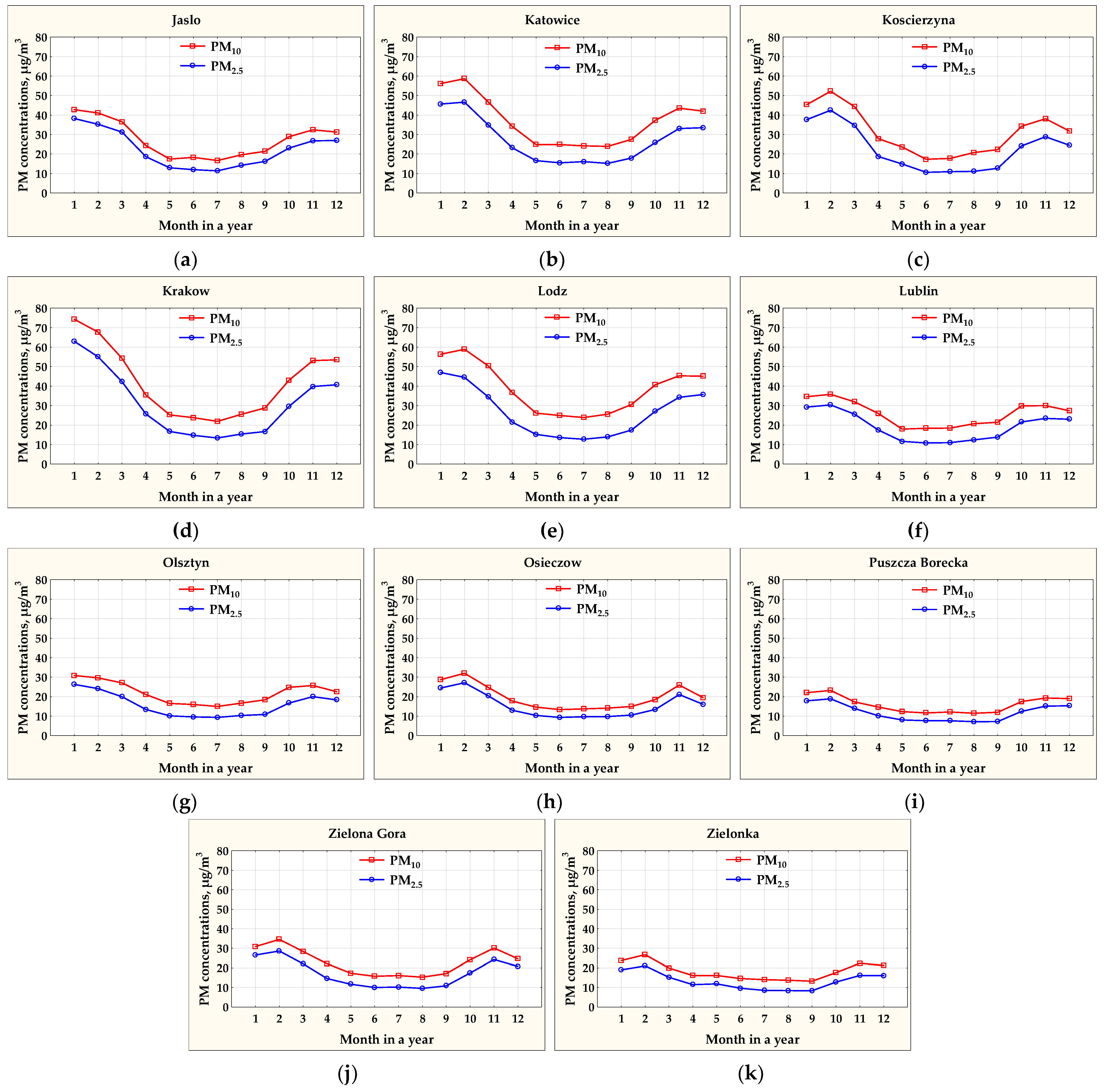
Based on many years of data recorded at the air monitoring stations, annual statistical patterns of PM2.5 and PM10 concentrations were calculated for each station. The plots of these patterns are presented in Figure 4. At all the stations, the lowest concentrations of suspended dust occurred in the spring/summer periods. In typical winter months, the particulate matter concentrations reached their highest values.

3.2. Correlations of Variables

A correlation analysis of the input variables, PM2.5, PM10 concentrations and date (D), was performed at each of the air monitoring stations. This analysis was performed to compare potential predictors of PM2.5 concentrations. The values of the Pearson correlation coefficients are presented in Table 3. The Pearson correlation coefficient ranges from −1 to 1; the closer to 1 or −1, the stronger the correlation between the variables. A positive sign means a positive correlation and a negative sign means a negative correlation. A coefficient value close to zero means a complete lack of correlation between the variables. At all the stations, the strongest correlations in relation to the PM2.5 concentration occurred for the PM10 concentration, much lower for the time variable D. These predictors were used to generate models I, II and III (see Section 2.5).

3.3. Results of Predicting PM2.5 Concentrations

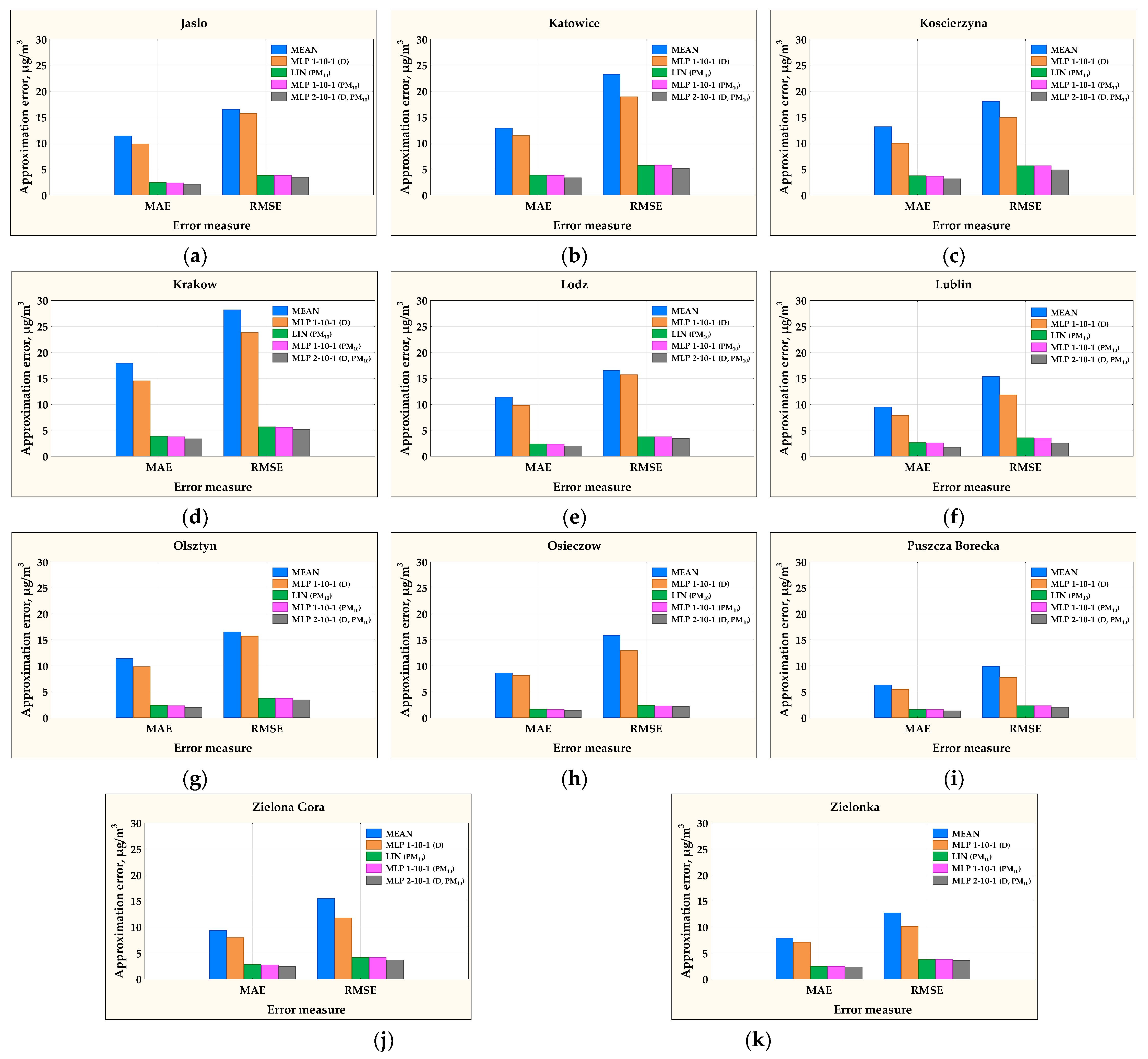
Modeling errors were calculated by comparing the predicted concentrations to the actual PM2.5 concentrations. Statistical prediction errors were calculated for each model variant separately for each air monitoring station. To evaluate the modeling accuracy, the five error measures defined by Formulas (1)–(5) were calculated. A summary of the prediction error values is presented in Table 4. The MAE and RMSE values are also presented graphically in Figure 5.
For all the stations, the largest modeling errors were achieved for the simplest neural models (Variant I), in which the only predictor was the time variable D (day). A very significant increase in the quality of modeling was noted for models in Variant II, in which the second predictor was the PM10 variable, strongly correlated with the explained variable PM2.5. These results are not surprising because PM10 is potentially the most important explanatory variable for PM2.5.
All naive MEAN models showed significantly lower accuracy than the MLP models. In turn, the LIN models were only slightly less accurate than the corresponding MLP models.
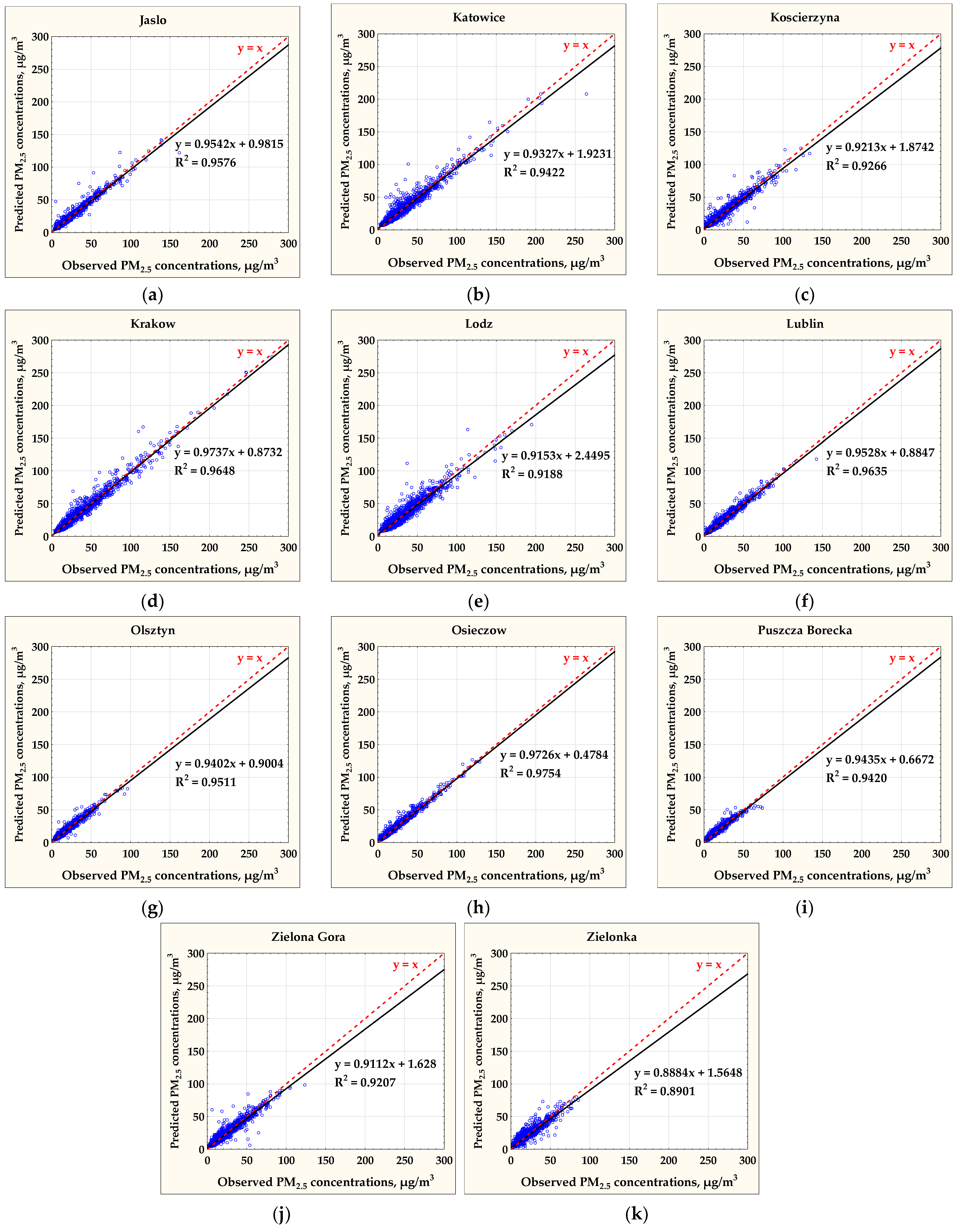
To compare the predicted and observed PM2.5 concentration values at different air monitoring stations, the corresponding scatterplots are shown in Figure 6. The results are presented for models with two predictors (Variant III: MLP 2-10-1). The perfect fit lines (red lines: y = x) and regression lines (black lines) are also shown in the scatterplots, as well as linear regression equations and determination coefficients.

3.4. Verification of the Models

Approach 1
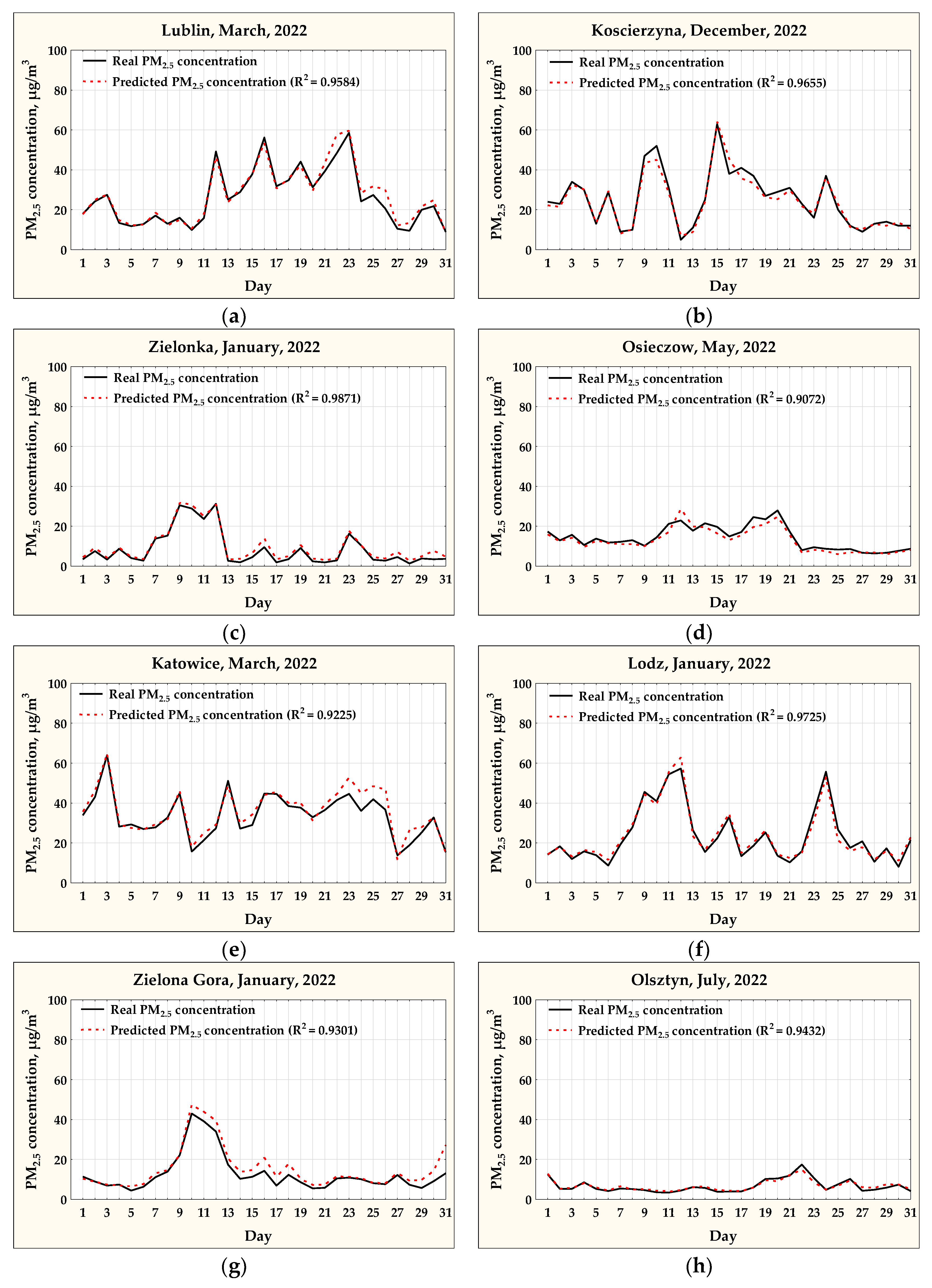
The usefulness of the considered ANN models was verified by computing trial forecasts for a period of one month, using models trained on data recorded in the past at the same station. Figure 7 shows predicted PM2.5 concentration courses for eight different locations and for different months in 2022. In each case, the network dedicated to a given station was used, i.e., the network trained on data from the same station. The graphs show actual courses and predicted PM2.5 concentration courses obtained using MLP 2-10-1 models with numeric date D and PM10 concentration as predictors (the most accurate model). For each selected period, the R2 value was calculated as a measure of the modeling accuracy.
Approach 2
In order to test the “universality” of the obtained MLP models, neural networks trained on data from one station were used to predict daily PM2.5 concentrations at other air monitoring stations. The models created for three air monitoring stations, Krakow, Osieczow and Olsztyn, were tested in this way, and the corresponding networks for Variant III (MLP 2-10-1) were used. For each monitoring station, the prediction capability of each of these three “foreign” models was assessed. The modeling errors were calculated for all the implementation cases, and the results are presented in Table 5, Table 6 and Table 7.

4. Summary and Discussion

The RMSE modeling errors compared to some PM2.5 and PM10 concentration statistics are presented in Table 8.
The modeling of PM2.5 concentrations using only the time variable D (Variant I) is burdened with significant prediction errors. However, such models have certain advantages over completely simple naive models such as mean models. In the naive mean model, all modeling results are the same and equal to the mean. The RMSE error of such modeling is equal to the standard deviation (SD) in the set of actual concentrations (the same formula). For models of Variant I (MLP 1-10-1), the RMSE values at individual stations were in the range of 7.79–23.8 μg/m3, while the standard deviations in the sets of actual PM2.5 concentrations were in the range of 8.6–28.0 μg/m3, depending on the station. SD always achieved values definitely higher than RMSE. The prediction day is always known and available, so a model in Variant I can be easily created. The time variable D brings information about the time of year to the models, and this is sufficient to improve the modeling quality compared to the mean model.
The implementation of PM10 concentration as an input significantly improved the quality of modeling at all stations (Variants II and III). RMSE values for models in Variant II were in the range of 2.31–6.86 μg/m3 and in Variant III in the range of 2.06–5.54 μg/m3. It should be emphasized that in the conditions occurring in Poland, the PM10 concentrations are usually strongly correlated with the PM2.5 concentrations (correlation coefficients ranged from 0.934 (Lodz) to 0.985 (Osieczow)). The values of other error measures also confirm that the Variant III models are the most accurate. Therefore, models MLP 2-10-1 can be recommended for use in practice.
Practical modeling needs may result from various reasons. There may be a need to supplement missing PM2.5 concentrations in data collected at air monitoring stations. The completeness of the PM2.5 concentration time series is required to assess air quality and is also the basis for assessing mortality rates, such as the number of premature deaths. Completing missing data on the concentrations of pollutants such as PM2.5 may be helpful in air quality management and environmental policy at local and regional levels.
Verification of the models in approach 1 showed the usefulness of the models in situations where historical data are available at the monitoring station. The results prove that models trained on historical data can be used to predict concentrations in periods other than those covered by measurements. In the episodes shown, which were randomly selected, the determination coefficients usually exceed 0.9 (Figure 7), which can be considered a good prediction quality. The prediction accuracy is only slightly inferior to the prediction accuracy determined for the tested measurement period.
Verification of the models in approach 2 was performed in order to test the “universality” of the obtained MLP models. Neural networks trained on data from one station were used to predict daily PM2.5 concentrations at other air monitoring stations. Three different models were tested. In each case, the relatively good quality of modeling at “foreign” monitoring stations was confirmed. The determination coefficients range from 0.880 to 0.971 for the Krakow model (Table 5), from 0.883 to 0.975 for the Osieczow model (Table 6) and from 0.712 to 0.951 for the Olsztyn model (Table 7). Each of the tested models retained the ability to make reasonable predictions, although the accuracies of some models were clearly worse than others. However, it was found that the models have a certain universality. This means that “foreign” models can be used for modeling, but the lower accuracy of such models should be taken into account.
The presented research addresses the possibility of modeling the 24 h PM2.5 concentrations, the so-called daily concentrations. Similar studies were previously carried out to check the possibility of modeling PM2.5 concentrations averaged over 1 h measurement periods, i.e., for the so-called hourly concentrations [54]. In the previously studied 1 h models, an additional time variable—hour—had to be taken into account. Hourly concentrations are characterized by much greater variability than daily concentrations, which is why they are more difficult to model. However, the addition of the H (hour) variable enabled reasonably accurate modeling of hourly PM2.5 concentrations. It was stated that neural regression models trained on the data from past years can be successfully used to model the current PM2.5 concentrations. The results presented in this study confirm this conclusion.
The main trend of research is the search for new, more and more accurate methods of modeling air pollution concentrations. Our research went in the opposite direction towards finding models that were as simple and universal as possible and could be used at most air monitoring stations. The only condition is to monitor PM10 concentrations. In our models, PM10 concentration is the primary predictor. We have shown that models trained at other air monitoring stations, the so-called foreign models, can be successfully used to approximate PM2.5 concentrations at a selected station. This is a novelty in modeling PM2.5 concentrations. This modeling method provides new possibilities in air quality assessment. Approximate concentrations of the PM2.5 fraction may be used to calculate mortality rates and other public health effects.
We are conscious of the limitations of the proposed methodology. The resulting models are accurate. The precision of these models can be improved, for example, by including additional predictors, such as concentrations of other pollutants, meteorological parameters and others. However, our goal was not to create the most accurate model possible. We were looking for models that were as simple as possible and highly accessible. We also wanted to test the possibility of building universal models.
Future research may aim to look for models that fit specific data.. Such research may lead to the use of more complex modeling tools, which have been described in many publications [51,52,53,65]. Research can also be conducted on segment modeling. Since differences in modeling accuracy were found in different concentration subranges [66,67], the improvement of modeling quality was tested by replacing a single model with a group of models dedicated to specific subranges of pollutant concentrations [68]. Promising results were obtained for segmented modeling.
The accuracy of the models can be increased by including other predictors that may influence PM concentration levels. These may be meteorological parameters affecting the emission of pollutants or the spread of pollutants in the air. Future research may also aim to find a more universal model that combines historical knowledge from measurements at various air monitoring stations.

Supplementary Materials

The following supporting information can be downloaded at: https://www.mdpi.com/article/10.3390/en17092202/s1.

Author Contributions

Conceptualization, S.H.; methodology, S.H. and R.J.; software, R.J. and J.B.; validation, R.J.; formal analysis, S.H. and R.J.; resources, R.J.; data curation, R.J.; writing—original draft preparation, S.H.; writing—review and editing, S.H., R.J. and J.B.; visualization, R.J.; project administration, S.H.; funding acquisition, S.H. All authors have read and agreed to the published version of the manuscript.

Funding

The research was funded by the statute subvention of the Czestochowa University of Technology Faculty of Infrastructure and Environment BS/PB-400-301 and Faculty of Electrical Engineering BS/PB-3-300-301.

Data Availability Statement

The data presented in this study are available on request from the corresponding author due to commercial restrictions.

Conflicts of Interest

The authors declare no conflicts of interest. The funders had no role in the design of the study; in the collection, analyses or interpretation of the data; in the writing of the manuscript; or in the decision to publish the results.

References

  1. Gurjar, B.R.; Molina, L.T.; Ojha, C.S.P. Air Pollution: Health and Environmental Impacts; CRC Press: Boca Raton, FL, USA, 2010. [Google Scholar]
  2. Kumar, P. Airborne Particles: Origin, Emissions and Health Impacts; Nova Science Publisher’s, Inc.: Hauppauge, NY, USA, 2017. [Google Scholar]
  3. Hoffmann, B.; Roebbel, N.; Gumy, S.; Forastiere, F.; Brunekreef, B.; Jarosinska, D.; Walker, K.D.; van Erp, A.M.; O’Keefe, R.; Greenbaum, D.; et al. A joint workshop report of ERS, WHO, ISEE and HEI. Eur. Respir. J. 2020, 56, 2002575. [Google Scholar] [CrossRef] [PubMed]
  4. Pandya, S.; Gadekallu, T.R.; Maddikunta, P.K.R.; Sharma, R. A Study of the Impacts of Air Pollution on the Agricultural Community and Yield Crops (Indian Context). Sustainability 2022, 14, 13098. [Google Scholar] [CrossRef]
  5. Wei, W.; Wang, Z. Impact of Industrial Air Pollution on Agricultural Production. Atmosphere 2021, 12, 639. [Google Scholar] [CrossRef]
  6. Agathokleous, E.; Frei, M.; Knopf, O.M.; Muller, O.; Xu, Y.; Nguyen, T.H.; Gaiser, T.; Liu, X.; Liu, B.; Saitanis, C.J.; et al. Adapting crop production to climate change and air pollution at different scales. Nat. Food 2023, 4, 854–865. [Google Scholar] [CrossRef] [PubMed]
  7. Chang, T.; Zivin, J.G.; Gross, T.; Neidell, M. Particulate Pollution and the Productivity of Pear Packers. Am. Econ. J. Econ. Policy 2016, 8, 141–169. [Google Scholar] [CrossRef]
  8. Graff-Zivin, J.; Neidell, M. The Impact of Pollution on Worker Productivity. Am. Econ. Rev. 2012, 102, 3652–3673. [Google Scholar] [CrossRef] [PubMed]
  9. Hanna, R.; Oliva, P. The Effect of Pollution on Labor Supply: Evidence from a Natural Experiment in Mexico City. J. Public Econ. 2015, 122, 68–79. [Google Scholar] [CrossRef]
  10. Aragon, F.; Miranda, J.; Oliva, P. Particulate Matter and Labor Supply: The Role of Caregiving and Non-linearities. J. Environ. Econ. Manag. 2017, 86, 295–309. [Google Scholar] [CrossRef]
  11. Conti, S.; Ferrara, P.; D’Angiolella, L.S.; Lorelli, S.C.; Agazzi, G.; Fornari, C.; Cesana, G.; Mantovani, L.G. The economic impact of air pollution: A European assessment. Eur. J. Public Health 2020, 30 (Suppl. 5), ckaa165.084. [Google Scholar] [CrossRef]
  12. Vallero, D.A. Fundamentals of Air Pollution, 4th ed.; Academic Press: Cambridge, MA, USA, 2008. [Google Scholar]
  13. Martinez, J. Great Smog of London. Encyclopedia Britannica, Article History. 27 February 2024. Available online: https://www.britannica.com/event/Great-Smog-of-London (accessed on 14 March 2024).
  14. Maesano, I. The Air of Europe: Where Are We Going? Eur. Respir. Rev. 2017, 26, 170024. [Google Scholar] [CrossRef]
  15. Tiotiu, A.I.; Novakova, P.; Nedeva, D.; Chong-Neto, H.J.; Novakova, S.; Steiropoulos, P.; Kowal, K. Impact of Air Pollution on Asthma Outcomes. Int. J. Environ. Res. Public Health 2020, 17, 6212. [Google Scholar] [CrossRef] [PubMed]
  16. Brito, F.F.; Gimeno, P.M.; Sánchez, J.F.; García, J.A.L.; Arias, T.A.; Ardanaz, J.M.U. Air Pollution and Asthma. In The Dangers of Allergic Asthma; García-Menaya, J.M., Ed.; Nova Science Publisher’s, Inc.: Hauppauge, NY, USA, 2023. [Google Scholar] [CrossRef]
  17. Kusumawardani, I.A.J.D.; Indraswari, G.; Komalasari, N.L.G.Y. Air Pollution and Lung Cancer. J. Respirasi 2023, 9, 150–158. [Google Scholar] [CrossRef]
  18. Berg, C.D.; Schiller, J.H.; Boffetta, P.; Cai, J.; Connolly, C.; Kerpel-Fronius, A.; Kitts, A.B.; Lam, D.C.; Mohan, A.; Myers, R.; et al. Air Pollution and Lung Cancer: A Review by International Association for the Study of Lung Cancer Early Detection and Screening Committee. J. Thorac. Oncol. 2023, 18, 10. [Google Scholar] [CrossRef] [PubMed]
  19. Brook, R.D.; Rajagopalan, S.; Pope, C.A., 3rd; Brook, J.R.; Bhatnagar, A.; Diez-Roux, A.V.; Holguin, F.; Hong, Y.; Luepker, R.V.; Mittleman, M.A.; et al. Particulate matter air pollution and cardiovascular disease: An update to the scientific statement from the American Heart Association. Circulation 2010, 121, 2331–2378. [Google Scholar] [CrossRef] [PubMed]
  20. Münzel, T.; Hahad, O.; Daiber, A.; Lelieveld, J. Luftverschmutzung und Herz-Kreislauf-Erkrankungen [Air pollution and cardiovascular diseases]. Herz 2021, 46, 120–128. (In German) [Google Scholar] [CrossRef]
  21. de Bont, J.; Jaganathan, S.; Dahlquist, M.; Persson, Å.; Stafoggia, M.; Ljungman, P. Ambient air pollution and cardiovascular diseases: An umbrella review of systematic reviews and meta-analyses. J. Intern. Med. 2022, 291, 779–800. [Google Scholar] [CrossRef] [PubMed]
  22. Li, J.; Xin, Y. Air Pollution and Cardiovascular Diseases. J. Am. Coll. Cardiol. 2023, 81, e97. [Google Scholar] [CrossRef] [PubMed]
  23. Peterson, B.S.; Rauh, V.A.; Bansal, R.; Hao, X.; Toth, Z.; Nati, G.; Walsh, K.; Miller, R.L.; Arias, F.; Semanek, D.; et al. Effects of Prenatal Exposure to Air Pollutants (Polycyclic Aromatic Hydrocarbons) on the Development of Brain White Matter, Cognition, and Behavior in Later Childhood. JAMA Psychiatry 2015, 72, 531–540. [Google Scholar] [CrossRef] [PubMed]
  24. Kim, Y.; Manley, J.; Radoias, V. Air Pollution and Long Term Mental Health. Atmosphere 2020, 11, 1355. [Google Scholar] [CrossRef]
  25. Calderón-Garcidueñas, L.; Ayala, A. Air Pollution, Ultrafine Particles, and Your Brain: Are Combustion Nanoparticle Emissions and Engineered Nanoparticles Causing Preventable Fatal Neurodegenerative Diseases and Common Neuropsychiatric Outcomes? Environ. Sci. Technol. 2022, 56, 6847–6856. [Google Scholar] [CrossRef]
  26. Peters, R.; Ee, N.; Peters, J.; Booth, A.; Mudway, I.; Anstey, K.J. Air Pollution and Dementia: A Systematic Review. J. Alzheimers Dis. 2019, 70, S145–S163. [Google Scholar] [CrossRef] [PubMed]
  27. Clean Air Act. UK Public General Acts, 5 July 1956. Available online: https://www.legislation.gov.uk/ukpga/Eliz2/4-5/52/enacted (accessed on 14 March 2024).
  28. Knox, A.; Evans, G.J.; Lee, C.J.; Brook, J.R. Air Pollution Monitoring and Sustainability. In Encyclopedia of Sustainability Science and Technology; Meyers, R.A., Ed.; Springer: New York, NY, USA, 2012. [Google Scholar] [CrossRef]
  29. Spandana, G.; Shanmughasundram, R. Design and Development of Air Pollution Monitoring System for Smart Cities. In Proceedings of the Second International Conference on Intelligent Computing and Control Systems (ICICCS), Madurai, India, 14–15 June 2018; pp. 1640–1643. [Google Scholar] [CrossRef]
  30. Xing, Y.F.; Xu, Y.H.; Shi, M.H.; Lian, Y.X. The impact of PM2.5 on the human respiratory system. J. Thorac. Dis. 2016, 8, E69–E74. [Google Scholar] [PubMed]
  31. Liu, G.; Li, Y.; Zhou, J.; Xu, J.; Yang, B. PM2.5 deregulated microRNA and inflammatory microenvironment in lung injury. Environ. Toxicol. Pharmacol. 2022, 91, 103832. [Google Scholar] [CrossRef] [PubMed]
  32. Behinaein, P.; Hutchings, H.; Knapp, T.; Okereke, I.C. The growing impact of air quality on lung-related illness: A narrative review. J. Thorac. Dis. 2023, 15, 5055–5063. [Google Scholar] [CrossRef] [PubMed]
  33. European Environment Agency. Air Quality in Europe-2020 Report. No. 12/2018; Publications Office of the European Union: Luxembourg, 2020.
  34. World Health Organization. New WHO Global Air Quality Guidelines Aim to Save Millions of Lives from Air Pollution. 2021. Available online: https://www.who.int/news/item/22-09-2021-new-who-global-air-quality-guidelines-aim-to-save-millions-of-lives-from-air-pollution (accessed on 14 March 2024).
  35. EN 12341:2014; Ambient Air—Standard Gravimetric Measurement Method for the Determination of the PM10 or PM2.5 Mass Concentration of Suspended Particulate Matter. iTeh, Inc.: Newark, DE, USA, 2014.
  36. Hammitt, J.K.; Morfeld, P.; Tuomisto, J.T.; Erren, T.C. Premature Deaths, Statistical Lives, and Years of Life Lost: Identification, Quantification, and Valuation of Mortality Risks. Risk Anal. 2020, 40, 674–695. [Google Scholar] [CrossRef] [PubMed]
  37. Ministry of Climate and Environment (Polish Government). Regulation on the Evaluation of Levels of Substances in the Air. 11 December 2020. Available online: http://isap.sejm.gov.pl/isap.nsf/DocDetails.xsp?id=WDU20200002279 (accessed on 12 March 2024). (In Polish)
  38. Milionis, A.E.; Davies, T.D. Regression and Stochastic Models for Air Pollution-I. Review, Comments and Suggestions. Atmos. Environ. 1994, 28, 2801–2810. [Google Scholar] [CrossRef]
  39. Manly, B.F.J. Statistics for Environmental Science and Management; Chapman & Hall/CRC: Boca Raton, FL, USA, 2001. [Google Scholar]
  40. Peng, G.; Leslie, L.M.; Shao, Y. Environmental Modeling and Prediction; Springer: Berlin/Heidelberg, Germany, 2002. [Google Scholar]
  41. Plaia, A.; Bondi, A.L. Single Imputation Method of Missing Values in Environmental Pollution Data Sets. Atmos. Environ. 2006, 40, 7316–7330. [Google Scholar] [CrossRef]
  42. Gardner, M.W.; Dorling, S.R. Artificial Neural Networks (the Multilayer Perceptron)-A Review of Applications in the Atmospheric Sciences. Atmos. Environ. 1998, 32, 2627–2636. [Google Scholar] [CrossRef]
  43. Dorling, S.R.; Gardner, M.W. Statistical Surface Ozone Models: An Improved Methodology to Account for Non-linear Behaviour. Atmos. Environ. 2000, 34, 21–34. [Google Scholar]
  44. Hoffman, S. Short-Time forecasting of atmospheric NOx concentration by neural networks. Environ. Eng. Sci. 2006, 23, 603–609. [Google Scholar] [CrossRef]
  45. Gentili, S.; Magnaterra, L.; Passerini, G. Handling Missing Data: Applications to Environmental Analysis; Latini, G., Passerini, G., Eds.; Wit Press: Southampton, UK, 2004. [Google Scholar]
  46. Hoffman, S. Missing data completing in the air monitoring systems by forward and backward prognosis methods. Environ. Protec. Eng. 2006, 32, 25–29. [Google Scholar]
  47. Hoffman, S. Treating missing data at air monitoring stations. In Environmental Engineering; Pawłowski, L., Dudzińska, M., Pawłowski, A., Eds.; Taylor & Francis Group: London, UK, 2007; pp. 349–353. [Google Scholar]
  48. Hoffman, S. Approximation of Imission Level at Air Monitoring Stations by Means of Autonomous Neural Models. Environ. Prot. Eng. 2012, 38, 109–119. [Google Scholar] [CrossRef]
  49. Lin, W.C.; Tsai, C.F. Missing value imputation: A review and analysis of the literature (2006–2017). Artif. Intell. Rev. 2020, 53, 1487–1509. [Google Scholar] [CrossRef]
  50. Shams, S.R.; Jahani, A.; Kalantary, S.; Moeinaddini, M.; Khorasani, N. The evaluation on artificial neural networks (ANN) and multiple linear regressions (MLR) models for predicting SO2 concentration. Urban Clim. 2021, 37, 100837. [Google Scholar] [CrossRef]
  51. Rijal, N.; Gutta, R.T.; Cao, T.; Lin, J.; Bo, Q.; Zhang, J. Ensemble of Deep Neural Networks for Estimating Particulate Matter from Images. In Proceedings of the IEEE 3rd International Conference on Image, Vision and Computing (ICIVC), Chongqing, China, 27–29 June 2018; pp. 733–738. [Google Scholar] [CrossRef]
  52. Chae, S.; Shin, J.; Kwon, S.; Lee, S.; Kang, S.; Lee, D. PM10 and PM2.5 real-time prediction models using an interpolated convolutional neural network. Sci. Rep. 2021, 11, 11952. [Google Scholar] [CrossRef] [PubMed]
  53. Zhang, B.; Rong, Y.; Yong, R.; Qin, D.; Li, M.; Zou, G.; Pan, J. Deep learning for air pollutant concentration prediction: A review. Atmos. Environ. 2022, 290, 119347. [Google Scholar] [CrossRef]
  54. Hoffman, S.; Jasiński, R. The Use of Multilayer Perceptrons to Model PM2.5 Concentrations at Air Monitoring Stations in Poland. Atmosphere 2023, 14, 96. [Google Scholar] [CrossRef]
  55. Duan, J.; Chen, Y.; Fang, W.; Su, Z. Characteristics and Relationship of PM, PM10, PM2.5 Concentration in a Polluted City in Northern China. Procedia Eng. 2015, 102, 1150–1155. [Google Scholar] [CrossRef]
  56. Colangeli, C.; Palermi, S.; Bianco, S.; Aruffo, E.; Chiacchiaretta, P.; Di Carlo, P. The Relationship between PM2.5 and PM10 in Central Italy: Application of Machine Learning Model to Segregate Anthropogenic from Natural Sources. Atmosphere 2022, 13, 484. [Google Scholar] [CrossRef]
  57. Chief Inspectorate of Environmental Protection (Poland)—Measurement Data Bank. Available online: https://powietrze.gios.gov.pl/pjp/archives (accessed on 12 March 2024).
  58. Statistica. Electronic Textbook, 1984–2017, Available in the STATISTICA 13.3 Program.
  59. Fletcher, R. Practical Methods of Optimization, 2nd ed.; John Wiley & Sons: New York, NY, USA, 2000. [Google Scholar]
  60. Broyden, C.G. The convergence of a class of double-rank minimization algorithms. J. Inst. Math. Its Appl. 1970, 6, 76–90. [Google Scholar] [CrossRef]
  61. Fletcher, R. A New Approach to Variable Metric Algorithms. Comput. J. 1970, 13, 317–322. [Google Scholar] [CrossRef]
  62. Goldfarb, D. A Family of Variable Metric Updates Derived by Variational Means. Math. Comput. 1970, 24, 23–26. [Google Scholar] [CrossRef]
  63. Shanno, D.F. Conditioning of quasi-Newton methods for function minimization. Math. Comput. 1970, 24, 647–656. [Google Scholar] [CrossRef]
  64. Willmott, C.J. On the validation of models. Phys. Geogr. 1981, 2, 184–194. [Google Scholar] [CrossRef]
  65. Li, X.; Peng, L.; Hu, Y.; Shao, J.; Chi, T. Deep learning architecture for air quality predictions. Environ. Sci. Pollut. Res. 2016, 23, 22408–22417. [Google Scholar] [CrossRef] [PubMed]
  66. Hoffman, S. Assessment of Prediction Accuracy in Autonomous Air Quality Models. Desalination Water Treat. 2015, 57, 1322–1326. [Google Scholar] [CrossRef]
  67. Hoffman, S. Estimation of Prediction Error in Regression Air Quality Models. Energies 2021, 14, 7387. [Google Scholar] [CrossRef]
  68. Hoffman, S.; Filak, M.; Jasiński, R. Air Quality Modeling with the Use of Regression Neural Networks. Int. J. Environ. Res. Public Health 2022, 19, 16494. [Google Scholar] [CrossRef]
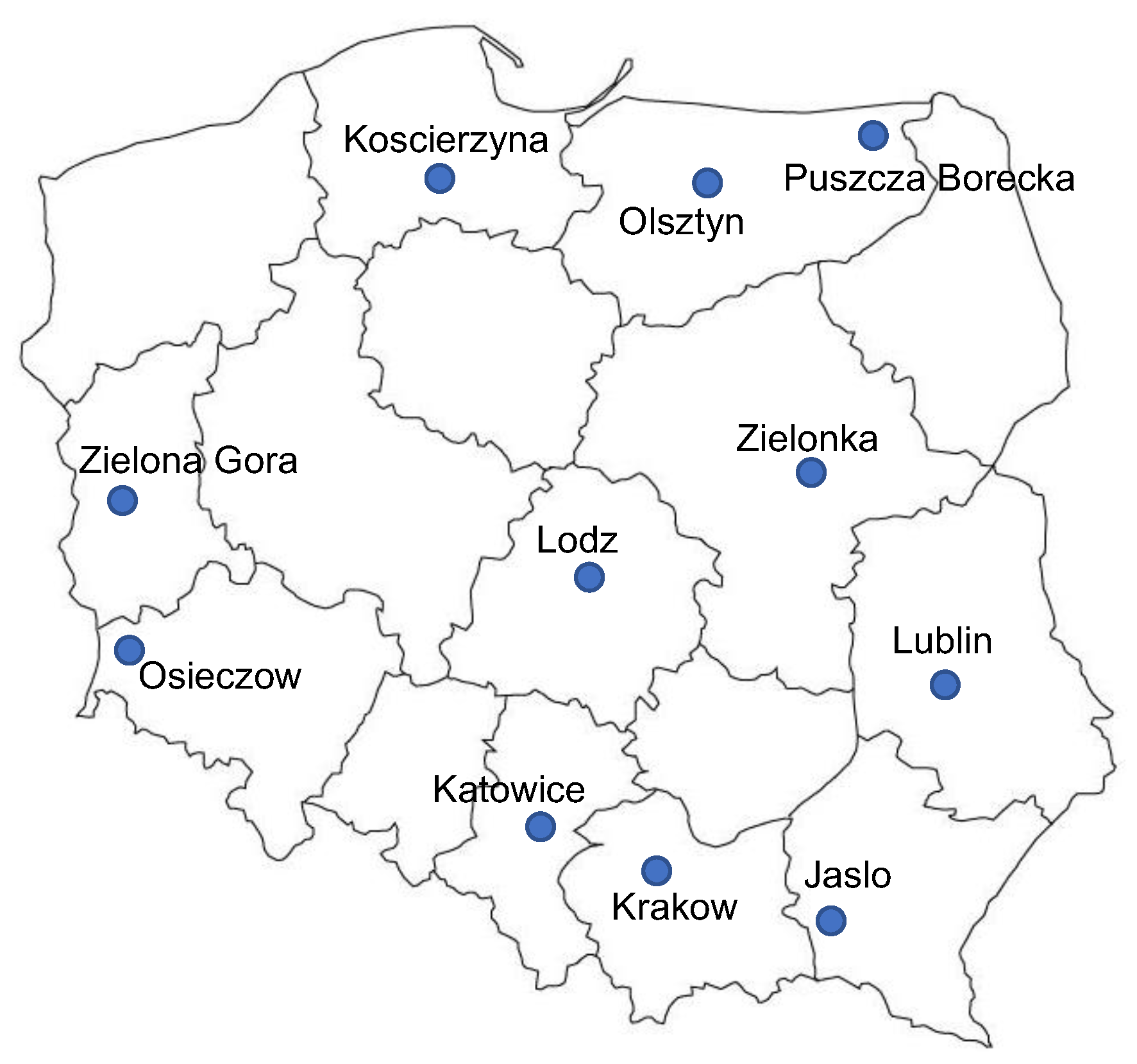
Figure 1. Map of Poland with locations of the air monitoring stations considered in the research.
Energies 17 02202 g001
Figure 2. Graphical presentation of basic statistical parameters of PM10 and PM2.5 concentrations from the considered air monitoring stations in 2010–2021: (a) PM10 concentrations, (b) PM2.5 concentrations. Values calculated after removing cases with missing data and for the years included in the analysis.
Energies 17 02202 g002
Figure 3. MLP architecture diagrams with 10 neurons in one hidden layer and 3 variants of predictors: (a) D; (b) PM10; (c) D, PM10.
Energies 17 02202 g003
Figure 4. Annual changes in PM10 and PM2.5 concentrations at the monitoring stations: (a) Jaslo, (b) Katowice, (c) Koscierzyna, (d) Krakow, (e) Lodz, (f) Lublin, (g) Olsztyn, (h) Osieczow, (i) Puszcza Borecka, (j) Zielona Gora, (k) Zielonka.
Energies 17 02202 g004
Figure 5. MAE and RMSE values for approximating PM2.5 concentrations in MEAN model, LINEAR model with PM10 as predictor and MLP models with D and PM10 predictors: (a) Jaslo, (b) Katowice, (c) Koscierzyna, (d) Krakow, (e) Lodz, (f) Lublin, (g) Olsztyn, (h) Osieczow, (i) Puszcza Borecka, (j) Zielona Gora, (k) Zielonka.
Energies 17 02202 g005
Figure 6. Scatterplots of predicted and observed PM2.5 concentrations for the MLP 2-10-1 models with D and PM10 predictors: (a) Jaslo, (b) Katowice, (c) Koscierzyna, (d) Krakow, (e) Lodz, (f) Lublin, (g) Olsztyn, (h) Osieczow, (i) Puszcza Borecka, (j) Zielona Gora, (k) Zielonka.
Energies 17 02202 g006
Figure 7. Example graphs of observed and modeled daily PM2.5 concentrations in selected months of 2022 using models of neural networks in Variant III (MLP 2-10-1), trained at the same station on the data from 2010 to 2021: (a) Lublin, March 2022; (b) Koscierzyna, December 2022; (c) Zielonka, January 2022; (d) Osieczow, May 2022; (e) Katowice, March 2022; (f) Lodz, January 2022; (g) Zielona Gora, January 2022; (h) Olsztyn, July 2022.
Energies 17 02202 g007
Table 1. Background information about the considered air monitoring stations, from [57].
Air Monitoring
Station
Address International
Code
Geographical
Coordinates, WGS84
Type of Station Area Type
JasloSikorskiego Str.PL0518AΦ 49.744886, λ 21.454617backgroundurban
Katowice6 Kossutha Str.PL0008AΦ 50.264611, λ 18.975028backgroundurban
KoscierzynaTargowa Str.PL0558AΦ 54.120694, λ 17.975861backgroundurban
KrakowBujaka Str.PL0501AΦ 50.010575, λ 19.949189backgroundurban
Lodz1 Legionow Str.PL0100AΦ 51.776417, λ 19.452936backgroundurban
Lublin5 Sliwińskiego Str.PL0085AΦ 51.273078, λ 22.551675backgroundurban
Olsztyn16 Puszkina Str.PL0175AΦ 53.789233, λ 20.486075backgroundurban
Osieczow(no street)PL0505AΦ 51.317630, λ 15.431719backgroundrural
Puszcza BoreckaDiabla GoraPL0005RΦ 54.124819, λ 22.038056backgroundrural
Zielona GoraKrotka Str.PL0213AΦ 51.939783, λ 15.518861backgroundurban
ZielonkaBory TucholskiePL0077AΦ 53.662136, λ 17.933986backgroundrural
Table 2. Completeness of the annual series of 24 h PM10 and PM2.5 concentrations for the years covered by the analysis, 2010–2021. Only values above 80% are shown.
Air Monitoring
Station
Total
Number of
Observations (Cases)
Completeness of the Annual Series
2010
%
2011
%
2012
%
2013
%
2014
%
2015
%
2016
%
2017
%
2018
%
2019
%
2020
%
2021
%
Jaslo2043----91.591.599.597.381.498.4--
Katowice2731----89.089.389.695.992.197.399.595.1
Koscierzyna1709----90.184.498.495.699.5---
Krakow2102----91.096.797.394.297.099.5--
Lodz2813----91.099.599.599.795.199.796.789.0
Lublin3229---96.790.4100.0100.0100.097.0100.0100.0100.0
Olsztyn2438-----95.995.694.089.097.397.398.4
Osieczow3412-95.395.6-88.894.886.391.597.089.997.097.8
Puszcza Borecka3413--92.991.887.194.891.395.197.596.293.494.2
Zielona Gora3849-89.992.994.892.991.899.797.5100.099.796.498.1
Zielonka376796.4100.089.199.289.0-89.187.198.496.492.993.7
Table 3. Pearson’s correlation coefficient for the input variables at individual air monitoring stations, 24 h average values, 2010–2021.
Air Monitoring StationVariableDPM10PM2.5
JasloD1.0000
PM100.42011.0000
PM2.50.47680.97351.0000
KatowiceD1.0000
PM100.38421.0000
PM2.50.44500.96391.0000
KoscierzynaD1.0000
PM100.44411.0000
PM2.50.50690.94871.0000
KrakowD1.0000
PM100.46891.0000
PM2.50.50480.97921.0000
LodzD1.0000
PM100.47551.0000
PM2.50.56610.93391.0000
LublinD1.0000
PM100.33191.0000
PM2.50.45530.96461.0000
OlsztynD1.0000
PM100.34321.0000
PM2.50.45190.94931.0000
OsieczowD1.0000
PM100.32191.0000
PM2.50.34430.98521.0000
Puszcza BoreckaD1.0000
PM100.34781.0000
PM2.50.43290.96111.0000
Zielona GoraD1.0000
PM100.37251.0000
PM2.50.44340.94871.0000
ZielonkaD1.0000
PM100.26621.0000
PM2.50.31760.93871.0000
Table 4. Values of modeling errors of PM2.5 concentrations in MEAN model, LINEAR model with PM10 as a predictor and MLP models with D and PM10 as predictors.
Air Monitoring
Station
Regression ModelExplanatory Variable (Predictors)MAE
μg/m3
RMSE
μg/m3
MARER2d
JasloMEAN-11.4316.550.68930.00000.0000
LINPM102.433.790.14000.94770.9864
MLP 1-10-1D9.8515.740.55150.23730.6155
MLP 1-10-1PM102.363.800.13210.94910.9867
MLP 2-10-1D, PM102.043.470.11480.95760.9890
KatowiceMEAN-12.9023.280.41610.00000.3162
LINPM103.875.730.16910.92920.9814
MLP 1-10-1D11.5018.950.51650.22360.5760
MLP 1-10-1PM103.845.810.16830.92740.9805
MLP 2-10-1D, PM103.355.180.15090.94220.9848
KoscierzynaMEAN-13.1818.040.97550.00000.0000
LINPM103.745.700.26680.90000.9732
MLP 1-10-1D10.0114.970.66930.30500.6807
MLP 1-10-1PM103.675.670.26750.90140.9735
MLP 2-10-1D, PM103.154.890.23390.92660.9805
KrakowMEAN-17.9628.200.78390.00000.1307
LINPM103.915.690.15760.95880.9894
MLP 1-10-1D14.5623.830.65390.27800.6492
MLP 1-10-1PM103.805.630.14970.95980.9897
MLP 2-10-1D, PM103.385.260.13400.96480.9910
LodzMEAN-13.1121.320.46140.00000.3499
LINPM104.866.940.22690.87220.9648
MLP 1-10-1D10.0515.630.45800.35220.7073
MLP 1-10-1PM104.746.860.21830.87540.9659
MLP 2-10-1D, PM103.765.540.18210.91880.9783
LublinMEAN-9.5015.380.44080.00000.3713
LINPM102.653.580.16920.93040.9817
MLP 1-10-1D7.9111.840.55030.23690.6047
MLP 1-10-1PM102.623.560.16400.93100.9820
MLP 2-10-1D, PM101.792.590.11610.96350.9905
OlsztynMEAN-7.7712.020.52670.00000.3059
LINPM102.513.580.17930.90120.9734
MLP 1-10-1D7.029.980.61970.23150.6118
MLP 1-10-1PM102.423.520.16830.90490.9742
MLP 2-10-1D, PM101.722.520.13010.95110.9872
OsieczowMEAN-8.6415.890.44560.00000.3434
LINPM101.702.430.14570.97050.9925
MLP 1-10-1D8.1812.950.77480.16210.5094
MLP 1-10-1PM101.582.310.13020.97330.9932
MLP 2-10-1D, PM101.482.220.12390.97540.9937
Puszcza BoreckaMEAN-6.359.960.48450.00000.3940
LINPM101.622.360.16920.92370.9798
MLP 1-10-1D5.527.790.69950.21880.5910
MLP 1-10-1PM101.612.340.17020.92550.9801
MLP 2-10-1D, PM101.382.060.14580.94200.9849
Zielona GoraMEAN-9.3315.500.43890.00000.3829
LINPM102.844.210.21070.90010.9732
MLP 1-10-1D7.9511.760.58970.22520.5708
MLP 1-10-1PM102.784.170.20580.90230.9734
MLP 2-10-1D, PM102.453.760.18120.92070.9787
ZielonkaMEAN-7.8712.750.56030.00000.3856
LINPM102.513.770.23760.88110.9675
MLP 1-10-1D7.1110.120.94100.12950.4835
MLP 1-10-1PM102.503.770.24450.88150.9676
MLP 2-10-1D, PM102.383.630.23850.89010.9701
Table 5. Prediction errors of 24 h PM2.5 concentrations at individual stations. Applied model: MLP 2-10-1 trained on data from Krakow, 2010–2021.
Air Monitoring
Station
Regression ModelExplanatory Variable (Predictors)MAE
μg/m3
RMSE
μg/m3
MARER2d
JasloMLP 2-10-1D, PM103.014.530.14630.95330.9796
KatowiceMLP 2-10-1D, PM103.405.380.14810.94010.9845
KoscierzynaMLP 2-10-1D, PM103.305.100.25140.92040.9785
KrakowMLP 2-10-1D, PM103.385.260.13400.96480.9910
LodzMLP 2-10-1D, PM104.136.210.20720.90460.9730
LublinMLP 2-10-1D, PM102.112.880.13690.95970.9877
OlsztynMLP 2-10-1D, PM102.042.840.16760.94080.9829
OsieczowMLP 2-10-1D, PM102.173.180.17860.97070.9852
Puszcza BoreckaMLP 2-10-1D, PM101.762.350.24610.93070.9784
Zielona GoraMLP 2-10-1D, PM102.633.950.19130.92030.9746
ZielonkaMLP 2-10-1D, PM102.663.810.33250.88000.9663
Table 6. Prediction errors of 24 h PM2.5 concentrations at individual stations. Applied model: MLP 2-10-1 trained on data from Osieczow, 2010–2021.
Air Monitoring
Station
Regression ModelExplanatory Variable (Predictors)MAE
μg/m3
RMSE
μg/m3
MARER2d
JasloMLP 2-10-1D, PM102.193.810.12150.95030.9872
KatowiceMLP 2-10-1D, PM104.247.760.18230.88860.9675
KoscierzynaMLP 2-10-1D, PM103.846.250.28640.91580.9720
KrakowMLP 2-10-1D, PM104.849.340.17900.90060.9712
LodzMLP 2-10-1D, PM105.698.430.28250.88260.9551
LublinMLP 2-10-1D, PM102.273.360.15140.95320.9853
OlsztynMLP 2-10-1D, PM102.263.470.17200.93150.9779
OsieczowMLP 2-10-1D, PM101.482.220.12390.97540.9937
Puszcza BoreckaMLP 2-10-1D, PM101.482.320.16110.93660.9823
Zielona GoraMLP 2-10-1D, PM102.614.030.19990.91500.9768
ZielonkaMLP 2-10-1D, PM102.534.090.24900.88420.9667
Table 7. Prediction errors of 24 h PM2.5 concentrations at individual stations. Applied model: MLP 2-10-1 trained on data from Olsztyn, 2010–2021.
Air Monitoring
Station
Regression ModelExplanatory Variable (Predictors)MAE
μg/m3
RMSE
μg/m3
MARER2d
JasloMLP 2-10-1D, PM103.315.760.15720.91340.9661
KatowiceMLP 2-10-1D, PM104.6111.340.16300.73710.9061
KoscierzynaMLP 2-10-1D, PM103.485.970.23600.89250.9692
KrakowMLP 2-10-1D, PM106.0315.860.15980.71190.8815
LodzMLP 2-10-1D, PM104.358.220.19100.82260.9472
LublinMLP 2-10-1D, PM102.143.760.12470.92810.9788
OlsztynMLP 2-10-1D, PM101.722.520.13010.95110.9872
OsieczowMLP 2-10-1D, PM102.063.630.14330.95000.9811
Puszcza BoreckaMLP 2-10-1D, PM101.482.170.15940.93600.9832
Zielona GoraMLP 2-10-1D, PM102.544.070.17610.90970.9741
ZielonkaMLP 2-10-1D, PM102.463.870.24050.87880.9678
Table 8. The RMSE modeling errors and some statistics on PM2.5 and PM10 concentrations for considered air monitoring stations.
Air Monitoring
Station
PM10,
μg/m3
PM2.5,
μg/m3
PM2.5/PM10
Ratio,
%
r-Pearson
PM2.5/PM10
RMSE,
μg/m3
MeanSDMeanSDVariant I
(MLP 1-10-1)
Variant III
(MLP 2-10-1)
Jaslo27.218.321.916.60.790.973515.743.47
Katowice36.626.526.721.50.710.963918.955.18
Koscierzyna31.421.122.818.00.700.948714.974.89
Krakow41.733.230.628.00.700.979223.835.26
Lodz38.822.526.519.40.660.933915.635.54
Lublin26.015.819.213.60.720.964611.842.59
Olsztyn22.013.615.711.40.700.94939.982.52
Osieczow19.915.315.514.10.740.985212.952.22
Puszcza Borecka16.010.311.78.60.710.96117.792.06
Zielona Gora23.014.717.213.30.720.948711.763.76
Zielonka18.413.313.310.90.710.938710.123.63
Disclaimer/Publisher’s Note: The statements, opinions and data contained in all publications are solely those of the individual author(s) and contributor(s) and not of MDPI and/or the editor(s). MDPI and/or the editor(s) disclaim responsibility for any injury to people or property resulting from any ideas, methods, instructions or products referred to in the content.