Article

Hybrid Approach for Detection and Diagnosis of Short-Circuit Faults in Power Transmission Lines

by
Luís Brito Palma
1,2
1
School of Science and Technology, NOVA University Lisbon, Campus de Caparica, 2829-516 Caparica, Portugal
2
CTS-Uninova & LASI, Campus de Caparica, 2829-516 Caparica, Portugal
Energies 2024, 17(9), 2169; https://doi.org/10.3390/en17092169
Submission received: 1 January 2024 / Revised: 3 April 2024 / Accepted: 25 April 2024 / Published: 1 May 2024
(This article belongs to the Section F: Electrical Engineering)

Abstract

:
In this article, the main problem under investigation is the detection and diagnosis of short-circuit faults in power transmission lines. The proposed fault detection (FDD) approach is mainly based on principal component analysis (PCA). The proposed fault diagnosis/identification (FAI) approach is mainly based on sliding-window versions of the discrete Fourier transform (DFT) and discrete Hilbert transform (DHT). The main contributions of this article are (a) a fault detection approach based on principal component analysis in the two-dimensional scores space; and (b) a rule-based fault identification approach based on human expert knowledge, combined with a probabilistic decision system, which detects variations in the amplitudes and frequencies of current and voltage signals, using DFT and DHT, respectively. Simulation results of power transmission lines in Portugal are presented in order to show the robust and high performance of the proposed FDD approach for different signal-to-noise ratios. The proposed FDD approach, implemented in Python, that can be executed online or offline, can be used to evaluate the stress to which circuit breakers (CBs) are subjected, providing information to supervision- and condition-based monitoring systems in order to improve predictive and preventive maintenance strategies, and it can be applied to high-/medium-voltage power transmission lines as well as to low-voltage electronic transmission systems.

1. Introduction

Electricity has been used as a major energy source since the late years of the 19th century. In 1891, three-phase alternating current transmission started in Germany, when a 175 km overhead power line was commissioned to supply electrical energy to an international electrical engineering exhibition located in Frankfurt [1]. Since high quantities of electrical energy are difficult to store, power transmission lines are needed to connect electrical power plants to electrical grids and consumer facilities.
Electrical power systems consisting of a great number of generation, transmission, and distribution subsystems are considered large complex systems; hence, their planning, design, modeling, installation, operation, and management are very difficult tasks [2,3,4]. Circuit breakers (CBs) are critical assets in power transmission systems; they are needed to control electrical power networks by switching circuits on, by carrying loads, and by switching circuits off in short-circuit faults or maintenance situations, under manual command or automatic supervision [5,6,7]. In recent decades, in typical overhead power transmission lines, network voltages have risen from 110 to 700 kV or more; typical nominal currents are of the order of several hundred amperes [8]. In SCADA systems, that supervise and control electrical power networks, fault detection and diagnosis (FDD) approaches and fault-tolerant control approaches must be implemented in order to try to guarantee that faults do not provoke drastic failures [9,10,11,12].
The occurrence of a short-circuit fault in a phase implies a rapid increase in current and a rapid decrease in voltage in that phase; in addition to these symptoms associated with amplitude variations, another relevant symptom is the rapid change in the frequency of these signals. Some relevant reviews related to state-of-the-art approaches for fault detection and diagnosis, with potential to be applied in power transmission lines, can be found in Refs. [13,14,15,16,17,18,19]. There exist two major approaches: (a) rule-based approaches, where rules are based on human expert knowledge; (b) data-driven machine learning (ML)/artificial intelligence (AI) approaches, where the algorithms independently detect and analyze data patterns and modify their behavior accordingly to predict new output.
The proposed rule-based robust FDD approach was developed in the context of the H2020 BD4NRG EU Project—Big Data for Next Generation Energy, https://www.bd4nrg.eu/ (accessed on 18 March 2024 ). It was found that the vast majority of references are associated with machine learning (ML)/artificial intelligence (AI) approaches; in this article, the great challenge was to propose a new rule-based hybrid FDD approach, with the advantage of being an easy-to-understand methodology based on signal processing and statistical analysis techniques. The main contributions of this article are (a) a fault detection approach based on principal component analysis in the two-dimensional scores space; and (b) a rule-based fault identification approach based on human expert knowledge, DFT, and DHT, combined with a probabilistic decision system. This is a hybrid rule-based approach in the sense that it combines different classical approaches such as principal component analysis for fault detection, discrete Fourier transform for fault identification via amplitude estimation, discrete Hilbert transform for fault recovery via instantaneous frequency estimation, and probabilistic decisions, without resorting to optimization techniques, in order to take advantage of the potential of each approach, with the aim of obtaining a high performance similar to the performances of ML/AI-based approaches.
The remaining parts of this article are organized as follows. Section 2 describes the state of the art. In Section 3, the theoretical concepts of the proposed robust rule-based fault detection and diagnosis approach are presented. Section 4 is dedicated to the presentation of the simulation results, a discussion regarding the performance of the new robust FDD approach, and also, a performance comparison with other approaches. Finally, in Section 5 the conclusions and directions for further research are presented.

2. State of the Art

This section starts with the presentation of the terminology and notation, covering topics of power systems and typical short-circuit faults, protection devices (relays and circuit breakers), and also typical fault detection and diagnosis approaches in this research area.

2.1. Terminology and Notation

Given that terminology is not always a consensual subject, it is important to clarify it when writing scientific articles. The terminology in the area of fault management used in this article can be found in Refs. [20,21], and also at the IFAC website https://tc.ifac-control.org/6/4/terminology/terminology-in-the-area-of-fault-management (accessed on 18 March 2024). In Table 1, the most relevant notation used in this article is presented.

2.2. Three-Phase Power Systems and Typical Faults

In three-phase power systems, the voltages and the currents can be modeled as sinusoidal signals for non-fault situations. In fault situations, the voltages and the currents are no longer sinusoidal signals, and assuming a simplified model can be expressed by (1) and (2) for a short period of time after the fault occurs, given that variations in amplitude, frequency, and phase will occur.
u ( k ) = A u ( k ) s i n ( w ( k ) k + ϕ ( k ) )
i ( k ) = A i ( k ) s i n ( w ( k ) k + ϕ ( k ) )
When an unintentional electrical connection occurs between two points at different potentials, a low-impedance loop is created, called a fault loop, in which a short-circuit current circulates [4,22]. Shunt (or short-circuit) faults are considered the most typical faults in power grids [23,24]. On high-voltage power networks, ground faults account for more than 80% of the total number of faults [25,26]. Ground faults are associated with both overcurrents and undervoltages in the affected phases (A, B, or C). The typical power system shunt (short-circuit) faults are [27] three-phase faults, three-phase-to-phase faults, three-phase-to-ground faults, and three-double-phase-to-ground faults.
Faults on high-voltage overhead power lines are generally single-phase-to-ground arcing faults and are mostly temporary; for this reason, protective circuit breakers are provided with the automatic reclosing function. This function allows the line to be reclosed and kept in operation after the fault has disappeared because the arc can self-extinguish [28]. The two main types of distribution network faults are transient faults and permanent faults, with about 80% being transient faults and 20% permanent faults [29].
High-impedance faults (HIFs) are very difficult to detect and recognize by traditional monitoring equipment because their presence results in a slight increase in load currents and a small decrease in the voltages [9,27,30].
The typical values of the signal-to-noise ratio (SNR) on power lines depends on the type, length, and load conditions, as well as the amplitudes and frequencies of signals and noise. According to [26], in the context of power lines, the noise is defined as an unwanted electrical signal with less than 200 kHz superimposed on the power system voltage or current in phase conductors, or found on neutral conductors or signal lines; it is not a harmonic distortion or transient, and it can disturb computers and controllers.

2.3. Circuit Breakers and Protective Relays

Circuit breakers are critical assets in power transmissions systems, since they are power devices used to control electrical power networks by switching circuits on, by carrying loads, and by switching circuits off in short-circuit faults or maintenance situations, under manual command or automatic supervision [5,6,7,31]. Typically, when a fault is detected in any of the three phases (A, B, or C), the circuit breaker opens the power contacts associated with the three phases (A, B, and C) for safety reasons. Since circuit breakers are critical assets in power transmission systems, new fault detection and diagnosis approaches should be developed and implemented in the SCADA systems of electricity distribution companies.
A protective relay is a device that monitors the electrical variables (voltages, currents, frequency, etc.) of power systems and triggers a circuit breaker to isolate the faulty element when a fault is detected. In recent years, a revolution has taken place in the development and application of microprocessor-based multifunction protective relays (MMPRs). Single-function electromechanical relays are now outdated, and these are being replaced with MMPRs in many industrial and utility systems [32].
In Figure 1, the fault times and circuit breaker actuation times are represented. Typically, the fault start is unknown, as is the case in the present work, although it can be estimated by analyzing the available signals. The fault detection time ( t 1 t 0 ) should be as short as possible, as the next tasks (FAI, CBO, CBC, and FAR) will only occur if the fault is detected. The fault detection and diagnosis approaches should be able to detect all the times: t 0 , t 1 , t i , t 2 , t 3 , and t 4 . The fault identification (FAI) task is the most complex.

2.4. Fault Detection and Diagnosis Approaches

In the last two decades there have been major developments in the areas of fault detection/diagnosis and fault-tolerant control due to increasing performance, quality, and sustainability requirements [12,33,34]. The first task is fault detection and the next is fault diagnosis [20]. Fault detection implies the determination of the faults present in the system, and the time of detection. In the context of this work, fault diagnosis implies the determination of the kind of the faults (fault identification), and also the fault times and circuit breaker actuation times, as depicted in Figure 1.
Reviews related to state-of-the-art approaches for fault detection and diagnosis that can be applied in power transmission lines can be found in [13,14,15,16,17,18,19]. There exist two major approaches: (a) rule-based approaches, where rules are based on human expert knowledge; and (b) data-driven machine learning/artificial intelligence approaches, where the algorithms independently detect and analyze data patterns and modify their behavior accordingly to predict new output.
Typical fault detection and diagnosis approaches applied to power transmission lines are as follows:
  • Rule-based signal processing approaches. Relevant studies include (a) phasor-based algorithms, time-domain analysis, time–frequency analysis (Fourier transform and wavelet transform) [28]; (b) approach based on positive sequence voltage and current measurement from phasor measurement units (PMUs) [35]; (c) harmonic analysis and use of discrete Fourier transform (DFT) [36]; (d) fault classification based on group sparse representation [37].
  • Rule-based statistical approaches. Relevant studies include (a) statistical fault detection approach based on the voltage energy signal (VES) [38]; (b) combination of symmetrical components technique with principal component analysis (PCA) for fault detection and classification [39].
  • Rule-based artificial intelligence approaches. Relevant studies include (a) fault detection based on fuzzy logic [40]; (b) approach based on fuzzy logic and wavelet transform [41]; (c) approach based on discrete wavelet transform and fuzzy decision system [42].
  • Data-driven machine learning/artificial intelligence approaches. Relevant studies include (a) fault detection and classification based on neural ELM networks [43]; (b) fault detection using the Pruned Exact Linear Time (PELT) algorithm in large datasets, and classification using wavelet transform [44]; (c) performance evaluation of different machine learning algorithms [45]; (d) different machine learning algorithms [28]; (e) automatic oscillography analysis with neural networks [46]; (f) variational autoencoders (VAEs) in conjunction with ML algorithms [47]; (g) empirical wavelet transform (EWT), local energy (LE), and support vector machine (SVM) [48]; (h) data-based Cauchy distribution weighting M-estimate RVFLNs neural method [30]; (i) review on artificial intelligence-based fault location methods in power distribution networks [18]; (j) fault location in power distribution systems via deep graph convolutional networks [49]; (k) fault identification based on deep reinforcement learning, using deep Q-network [50].
In Table 2, relevant modern references in the FDD area applied to power transmission lines are mentioned, sorted by year. In the bibliographical research carried out, it was found that the vast majority of references are associated with ML/AI approaches; in this article, the great challenge was to propose a new rule-based FDD approach. At the end of Section 4, the proposed FDD approach is compared to all these FDD approaches, in terms of fault identification performance.
In a great number of situations, the fault detection and diagnosis (FDD) problem can be formulated as a classification problem that maps the symptoms into faults, taking into consideration the reference patterns associated with the nominal situation without faults [10]. This was the approach followed in this article, using a rule-based classification approach. The SCADA supervision systems with fault-tolerance capabilities must try to guarantee that the systems remains in the region of required performance and safety, even in faulty situations [10,11]. Protective circuit breakers provided with the automatic reclosing function allow, in many situations, fault (short-circuit) recovery in less than 1 s, as will be detailed in Section 4.

3. Proposed Fault Detection and Diagnosis Approach

This section contains the following topics: (a) HyperSim simulator and COMTRADE files; (b) nominal operation, SNR, short-circuit faults, and main symptoms; (c) the proposed theoretical fault detection and diagnosis architectures and approaches.

3.1. HyperSim Simulator and COMTRADE Files

In this work, a big dataset with relevant short-circuit faults was used, made available by the R&D Nester laboratory (https://www.rdnester.pt/en-GB (accessed on 18 March 2024)) from the REN TSO electricity infrastructure (“Redes Elétricas Nacionais”, https://www.ren.pt/en-gb (accessed on 18 March 2024)), in the context of the H2020 BD4NRG EU Project—Big Data for Next Generation Energy, https://www.bd4nrg.eu/ (accessed on 18 March 2024). The HyperSim simulator (https://www.opal-rt.com/systems-hypersim/ (accessed on 20 March 2024)) was used to create models of 12 overhead power lines in Portugal, with different voltages (150 kV, 220 kV, and 400 kV). These models were developed by the R&D Nester laboratory, the synthetic data were saved in 619 COMTRADE files, and after converted to the CSV format that was used in this work [46].
The IEEE Standard C37.111 (https://standards.ieee.org/ieee/C37.111/3795/ (accessed on 20 March 2024)), also known as IEC 60255-24 Ed.2, defines a common format for transient data exchange, COMTRADE (common format for transient data exchange), for power systems; it was developed to provide a standard file format for sampled analog waveforms and event data collected by monitoring devices [27]. COMTRADE files enable the exchange of data files between incompatible devices.

3.2. Nominal Operation, SNR, Short-Circuit Faults, and Main Symptoms

On overhead power lines, in the nominal operating region (without short-circuit faults), the neutral current i 0 should obey the condition expressed by Equation (3). When the current exceeds the rating of the differential circuit breaker, approximately 1 A or a few amperes, the differential circuit breaker opens the power contacts; in this work, the estimation of the fault start instant t 0 is based on the instant at which | ( i 0 ( k ) | > 1 A. The grounded (earthed) neutral wire can also serve as a parallel path to earth for short-circuit fault currents, acting as a neutral fault protection.
| i 0 ( k ) | < 1 A
Harmonics in power lines are mainly due to the use of nonlinear power electronics equipment, causing voltage distortions and affecting the quality of energy supplied to consumers. According to EN-50160/IEC-61000-3-2 standards, the total harmonic distortion (THD) limit value for voltages above 1000 V is 5%; this value is valid for nominal (normal) operating conditions with a probability of 95%.
In this work, in order to emulate some of the situations referred to as load imbalances, load variations, and voltage distortions, Gaussian noise was added to the voltage and current signals, assuming different signal-to-noise ratios (SNRs), as detailed in Table 3, since the available signals generated by the HyperSim simulator, made available by the R&D Nester laboratory, do not contain noise. The lowest SNR values (25 dB and 20 dB) were established taking into account typical allowable tolerances in voltage and current signals in nominal operation; they were 5% and [10%; 20%].
In a power line, when a short-circuit fault occurs, two typical relevant symptoms are the rapid increase in current and the rapid decrease in voltage [9,27]. Based on this premise, for the faults under study, Table 4 was constructed, which defines the rules used in this work for fault detection and diagnosis; a rapid increase in the current is denoted using the label “+1”, and a rapid decrease in the voltage is denoted using the label “−1”; the label “0” denotes a symptom not relevant to fault diagnosis.
In the event of a short-circuit fault, in addition to the symptoms of rapid changes in the amplitudes of currents and voltages, another relevant symptom is the rapid change in the frequency of these signals.

3.3. High-Level Architecture of the Proposed Fault Detection and Diagnosis Approach

In Figure 2, the high-level architecture of the proposed fault detection and diagnosis approach is depicted. As detailed in Section 3.1, a big dataset with relevant short-circuit faults was generated by the HyperSim simulation software, allowing access to three-phase voltage and current signals in power lines, Ux and Ix . The fault detection approach is based on applying linear principal component analysis (PCA) to voltage signals, detecting deviations from the nominal PCA model (without short-circuit faults); here, it is assumed that the fault is detected at time t 1 . The fault diagnosis approach is mainly based on estimating the instantaneous amplitude (Ae) and instantaneous frequency (Fe) of the voltage and current signals, using the discrete Fourier transform (DFT) and the discrete Hilbert transform (DHT), respectively; in addition to identifying the type of short-circuit fault (F1-“CG”, F2-“BG”, etc.), this proposed methodology made it possible also to identify the various time instants at which the fault was identified ( t i ), the circuit breaker opening ( t 2 ), the circuit breaker closing ( t 3 ), the fault recovery ( t 4 ), the actuation delay ( t 2 t 0 ), and the reconnection time ( t 4 t 2 ).
In the next sections, detailed architectures for fault detection and for fault diagnosis will be presented and explained.

3.4. Fault Detection Approach

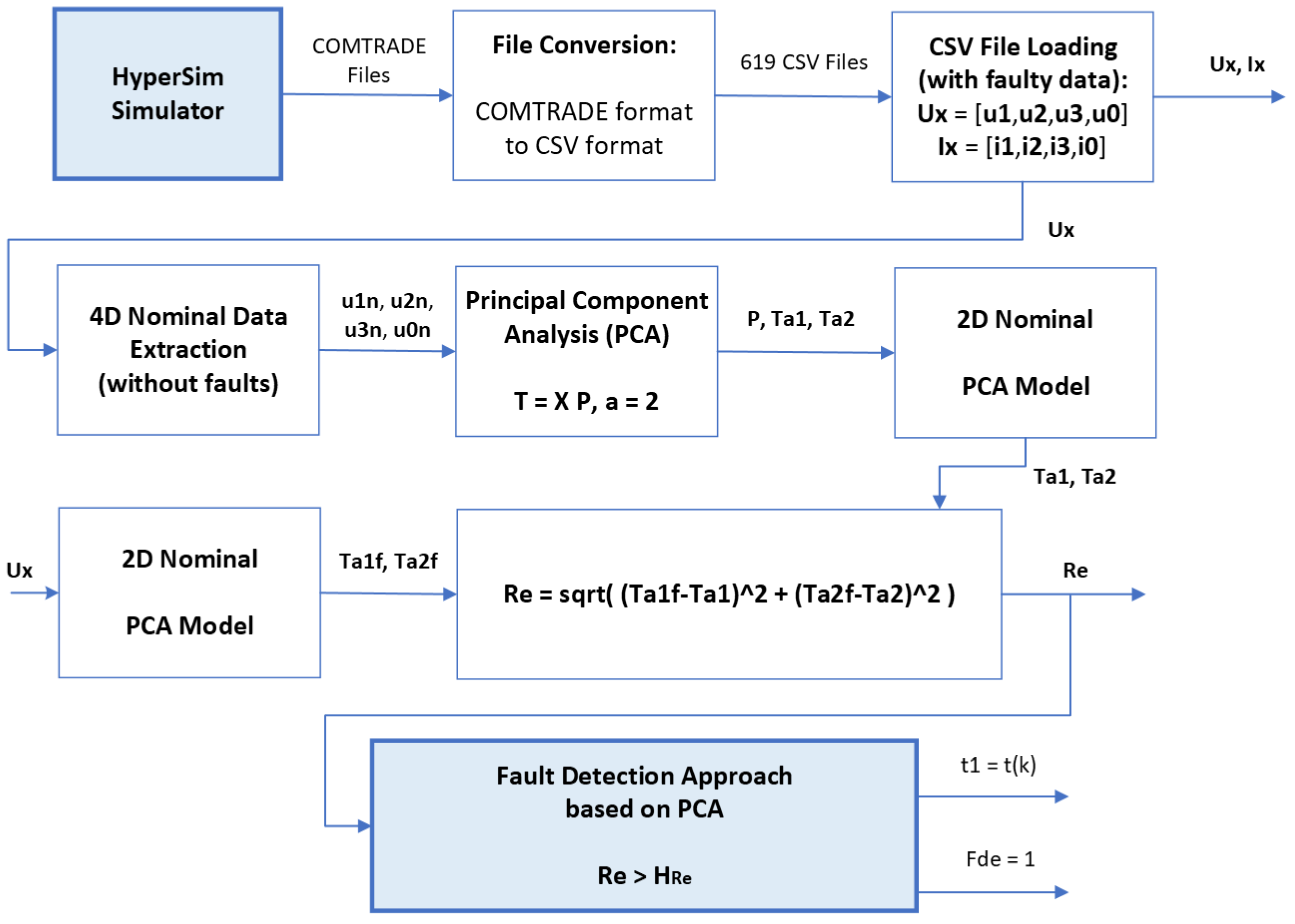
In Figure 3, the detailed architecture of the proposed fault detection approach is depicted. The fault detection approach is based on applying linear principal component analysis (PCA) to voltage signals ( u 1 , u 2 , u 3 , u 0 ), given that voltage signals present a high level of correlation under nominal (fault-free) operating conditions. When a fault occurs, in our case a short-circuit fault, the correlation level decreases profoundly and quickly.
In dynamic processes where correlation or redundancy between variables exists, it is advantageous to reduce the number of variables, maintaining an important quantity and quality of relevant original information. Dimensionality reduction techniques, such as principal component analysis (PCA), can greatly simplify and improve process monitoring tasks, since they project the data into a lower-dimensional space that accurately characterizes the state of the process under study [34,51,52,53,54]. Principal component analysis (linear PCA) is one of the most popular dimensionality reduction techniques. PCA is a multivariate statistical technique in which a number of related variables are transformed to a smaller set of uncorrelated variables. PCA preserves the correlation structure between the process variables, and captures the variability in the data. Principal component analysis is a multivariate statistical technique that can also be used to design linear controllers [55,56] or nonlinear controllers [57].
Next, the methodology proposed for applying linear PCA to voltage signals is described, based on PCA and implemented using singular value decomposition (SVD) [10]. Given a training set of n observations and m process variables stacked into a data matrix X n × m , the loading vectors are computed by solving the stationary points of the optimization problem formulated in Equation (4), where v m × 1 [34].
m a x v 0 v T X T X v v T v
The stationary points of Equation (4) can be computed via singular value decomposition (SVD) as described in Equation (5), where U n × n and V m × m are unitary matrices, and the matrix Σ n × m contains the non-negative real singular values of decreasing magnitude along its main diagonal σ 1 σ 2 . . . σ m i n ( m , n ) ) 0 , and zero off-diagonal elements. The loading vectors are the orthonormal column vectors in the matrix V , and the variance in the training set projected along the i t h column of V is equal to σ i 2 .
1 n 1 X = U Σ V T
Solving Equation (5) is equivalent to solving an eigenvalue decomposition of the sample covariance matrix S , as described in Equation (6), where the diagonal matrix Λ = Σ T Σ , with Λ m × m , contains the non-negative real eigenvalues of decreasing magnitude λ 1 λ 2 . . . λ m 0 , and the i t h eigenvalue equals the square of the i t h singular value, λ i = σ i 2 [34].
S = 1 n 1 X T X = V Λ V T
In a great number of practical applications, and also in this work, one of the goals is to minimize the effect of random noise, or high-frequency disturbance signals, that can corrupt the PCA representation, and to optimally capture the relevant variations in the data. To achieve this goal, only the loading vectors associated with the a largest singular values must be retained in the PCA model. PCA projects the observation space into two subspaces: the scores subspace, and the residual subspace. Selecting the columns of the loading matrix P m × a to correspond to the loading vectors V m × m associated with the a largest singular values, the projections of the observation data X n × m into the lower-dimensional space are contained in the scores matrix T n × a , as described in Equation (7), and the projection of T back into the m-dimensional observation space X ^ is given by Equation (8).
T = X P
X ^ = T P T
The residual matrix E is computed according to Equation (9) and captures the variations in the observation space spanned by the loading vectors associated with the m a smallest singular values. Typically, the two subspaces spanned by X ^ and E are denominated the scores space and residual space, respectively. A more accurate representation of the process is given by the scores space, since residual spaces that have a small signal-to-noise ratio (SNR) are removed.
E = X X ^
For a linear PCA model, the amount of variance explained by a principal components is given by Equation (10), that depends on the eigenvalues λ i of the matrix Λ obtained in Equation (6) by SVD, assuming that m is the number of process variables [34,52].
E σ 2 ( a ) [ % ] = i = 1 a λ i i = 1 m λ i × 100 %
In the PCA approach, the number of dimensions of the reduced space a defines the number of dimensions of the scores space. One way to define this number of dimensions a is to choose a number of dimensions that explains a high percentage of the total variance in the features data, for example, 80 % or more. For many applications, only two or three principal components are retained in the PCA model [10,34].
In this work, only the scores space T was selected for implementing the short-circuit fault detection approach, considering only two principal components, a = 2 , for m = 4 process variables (nominal voltage signals u 1 n , u 2 n , u 3 n and u 0 n ); this decision was based on the high variance explained by the first two principal components, as described in Table 5, for high-SNR voltage signals.
A big dataset with relevant short-circuit faults was generated by the HyperSim simulation software, allowing access to three-phase voltage and current signals in power lines, U x = [ u 1 u 2 u 3 u 0 ] and I x = [ i 1 i 2 i 3 i 0 ] , as described in Section 3.1. Each one of the 619 files generated by the HyperSim software recorded a simulation lasting t m a x = 1.5 s, including the occurrence of one of the seven short-circuit faults described in Table 4; given that the sampling interval was T s = 50 µs, the number of samples in each signal was n = 30,001.
Based on the SVD and PCA concepts described in this section, it is now possible to present in detail the proposed short-circuit fault detection approach. The data matrix X n n × m ( n =  30,001, m = 4 ) used to build the nominal PCA model is given by Equation (11), containing the nominal voltages (without short-circuit faults) in each phase and in the neutral wire. The covariance matrix S n m × m ( m = 4 ) is described in Equation (12). The loading matrix P a m × a ( m = 4 , a = 2 ) corresponds to the loading vectors V m × m associated with the a largest singular values, expressed by Equation (13). The projections of the observation data X n × m into the lower-dimensional space are contained in the scores matrix T a n × a ( n =  30,001, a = 2 ) , as described in Equation (14).
X = X n = u 1 n ( 0 ) u 2 n ( 0 ) u 3 n ( 0 ) u 0 n ( 0 ) u 1 n ( 1 ) u 2 n ( 1 ) u 3 n ( 1 ) u 0 n ( 1 ) u 1 n ( n 1 ) u 2 n ( n 1 ) u 3 n ( n 1 ) u 0 n ( n 1 )
S = S n = 1 n 1 X T X = V Λ V T
P = P a = V m , a
T = T a = X n P a
Human beings only have the ability to monitor signals well in one or two dimensions [10]. In this work, the PCA analysis allowed a reduction in the dimensionality of the problem from m = 4 to a = 2 . Given that the choice was a = 2 (two principal components), the scores space is a two-dimensional (2D) space, i.e., T a = T 2 , so we have a 2D nominal PCA model. In this 2D scores space, the scores matrix for a window of length n can be represented by two column vectors Equation (15). Each line of T a is a score, and each score is a projection of the original data in the 2D reduced scores space; the score with coordinates ( t a 1 ( k ) , t a 2 ( k ) ) , with k { 0 , 1 , . . . , n 1 } , is represented by a point in the two-dimensional scores space.
T a = T 2 = [ t a 1 t a 2 ] = t a 1 ( 0 ) t a 2 ( 0 ) t a 1 ( 1 ) t a 2 ( 1 ) t a 1 ( k ) t a 2 ( k ) t a 1 ( n 1 ) t a 2 ( n 1 )
PCA models have the advantage that the scores variables produced, which are linear combinations of the original variables, are more normally distributed than the original variables themselves; this is a consequence of the central limit theorem. For problems where the data obeys a normal distribution, the threshold of the two-dimensional scores space is an ellipse, according to the T2 statistics, given by Equation (16), where T α 2 depends on Fisher’s F-distribution with m and n m degrees of freedom [10,34].
( t a 1 ( k ) ) 2 λ 1 + ( t a 2 ( k ) ) 2 λ 2 = T α 2
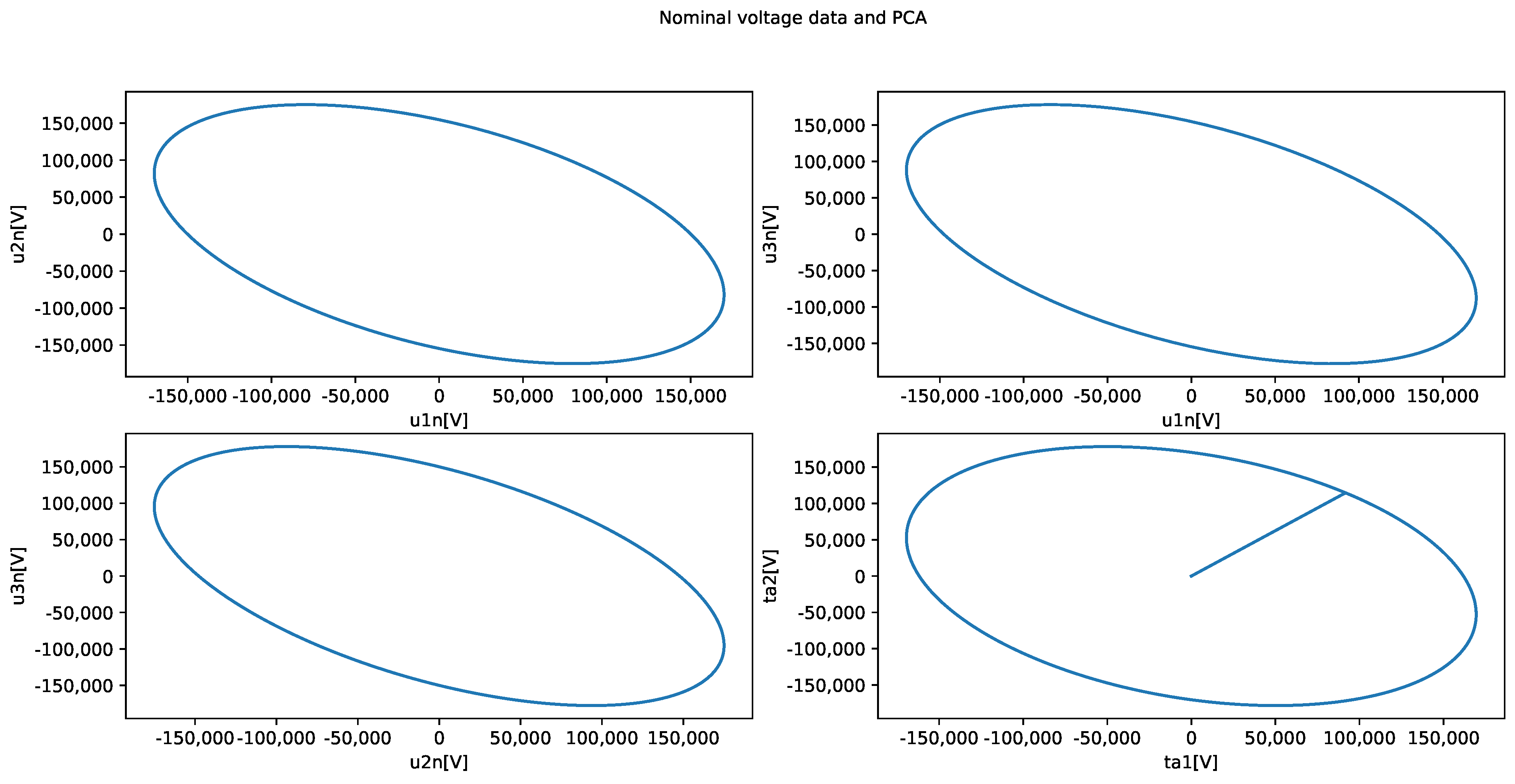
For the problem under study, the 2D graphics that relate the sinusoidal nominal voltage signals ( u 1 n , u 2 n , u 3 n ), for data in the nominal operating region (without short-circuit faults), are inclined ellipses, as depicted in Figure 4; in this figure, it can also be verified that the nominal PCA model in the 2D scores space [ t a 1 t a 2 ] , for data in the nominal operating region, is also an inclined ellipse. This nominal PCA model in the 2D scores space [ t a 1 t a 2 ] , an inclined ellipse, is proposed in this work as the reference model for fault detection, as detailed next.
For each time sample k, a short-circuit fault is detected if the signal R e ( k ) given by Equation (17) exceeds the threshold, i.e., the condition expressed in Equation (18) is verified. An adaptive threshold was used in this approach, H R e ( k ) , that depends on the SNR computed in the nominal operating region (without faults), expressed by Equation (21) and assuming G d = 1.2 , a value detailed later. Equation (17) expresses the distance between two points (two scores) in the scores space, the current score ( T a 1 f ( k ) , T a 2 f ( k ) ) and the nominal score ( T a 1 ( k ) , T a 2 ( k ) ) , as described in Equation (19) and in Equation (20), respectively, taking into account Equation (14).
R e ( k ) = ( t a 1 f ( k ) t a 1 ( k ) ) 2 + ( t a 2 f ( k ) t a 2 ( k ) ) 2
R e ( k ) > H R e ( k )
[ t a 1 f ( k ) t a 2 f ( k ) ] = [ u 1 ( k ) u 2 ( k ) u 3 ( k ) u 0 ( k ) ] P a
[ t a 1 ( k ) t a 2 ( k ) ] = [ u 1 n ( k ) u 2 n ( k ) u 3 n ( k ) u 0 n ( k ) ] P a
H R e ( k ) = G d × m a x ( R e ( k N + 1 : k ) )

3.5. Fault Diagnosis Approach

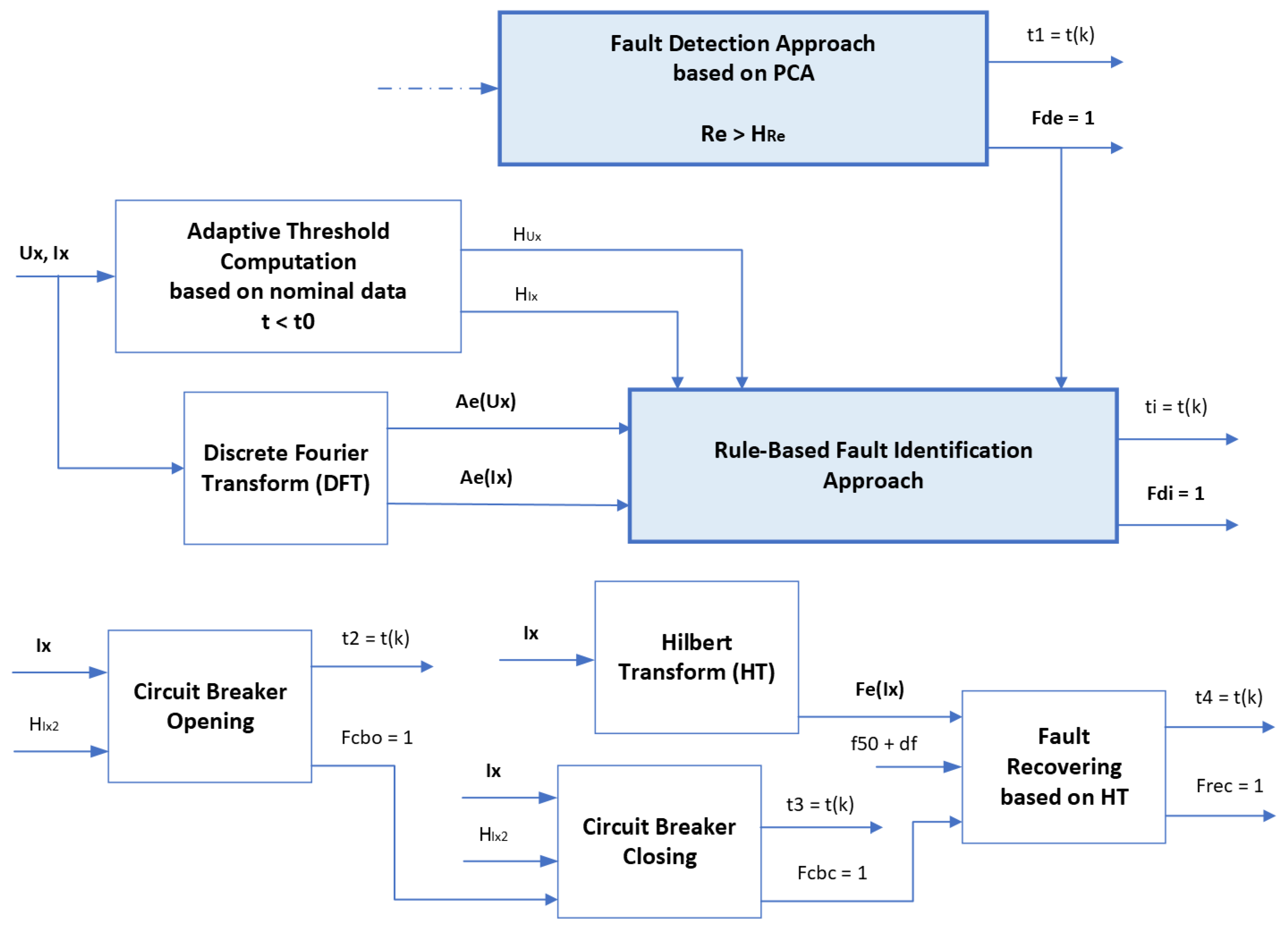
In Figure 5, the detailed architecture of the proposed fault diagnosis approach is depicted, including the final stage of the fault detection approach, in order to clarify the link between them. Taking into account the actions and respective times defined in Figure 1, the fault diagnosis stage can be divided into four tasks: (a) rule-based fault identification using the DFT for amplitude estimation, combined with a probabilistic decision system; (b) circuit breaker opening; (c) circuit breaker closing; (d) fault recovery using the DHT for instantaneous frequency estimation. Each of these tasks will be explained in different subsections.

3.5.1. Rule-Based Fault Identification

In order to increase the accuracy of the rule-based fault identification approach, for different SNR conditions, a probabilistic decision system was developed and implemented according to the architecture detailed in Figure 6, as described next.
As described in Section 3.2, when a short-circuit fault occurs in a power line, two typical relevant symptoms are the rapid increase in current and the rapid decrease in voltage. In this work, Table 4 was constructed reflecting this premise, and it is the base structure used here to create the if–then rules for fault identification.
In order to facilitate the explanation of the fault identification approach, a summarized version of Table 4 is presented here in Table 6, with only faults F5, F1, and F0. To implement the if–then rules, it is necessary to estimate the amplitudes of current signals [ i 0 i 1 i 2 i 3 ] and voltage signals [ u 1 u 2 u 3 ] , within a sliding window of length N. In the present work, this task was achieved by using a sliding-window version of the discrete Fourier transform (SW-DFT), implementing an algorithm with overlapping windows to reduce artifacts at the boundary, as a discrete short-time Fourier transform (DSTFT), according to Equation (22), for a discrete-time signal x ( k ) with N points; using smaller time frames, the frequency spectrum moves more smoothly over time; therefore, it is more accurate [58]. The DSTFT can be used to analyze how the frequency content of a nonstationary signal changes over time. If we attempt to compute the DFT over a non-integer number of cycles of the input signal, then we might expect the transform to be corrupted in some way; so, in this work, two cycles were used to compute the SW-DFT, corresponding to N = 800 samples.
X ( Ω n ) = k = 0 N 1 x ( k ) e j Ω n k , Ω n = 2 π N n
By way of example, in Equation (23) the condition for identification of fault F5 (ACG) at time instant t i = t ( k ) is expressed, ensuring t i > t 1 , according to Table 6, using the estimated amplitudes of the current signals and the voltage signals based on the SW-DFT transform; this approach was implemented in a robust way, as explained next. The diagnosis of other short-circuit faults is carried out in a similar way, following the rules formally defined in Table 4.
As currents in power lines depend on loads, it was necessary to implement an adaptive thresholds approach, H x , according to (24) and (25). A sliding-window of length N was considere, in the nominal operating region before the fault detection time t 1 , i.e., k n < k 1 and k 1 = t 1 / T s . The absolute value function is represented by | | , and the maximum function is represented by m a x ( ) . The typical allowable tolerances in voltage and current signals in nominal operation are, respectively, 5% and [10%; 20%]. The 20% tolerance allowed us to define the gain G i = 1.2 , and the 5% tolerance allowed us to define the gain G u = 0.95 .
( i 0 a ( k ) > H i 0 ) & & ( i 1 a ( k ) > H i 1 ) & & ( i 2 a ( k ) < H i 2 ) & & ( i 3 a ( k ) > H i 3 ) & & ( u 1 a ( k ) < H u 1 ) & & ( u 3 a ( k ) < H u 3 )
H i x = G i m a x ( i x ( k n N + 1 : k n ) )
H u x = G u m a x ( u x ( k n N + 1 : k n ) )
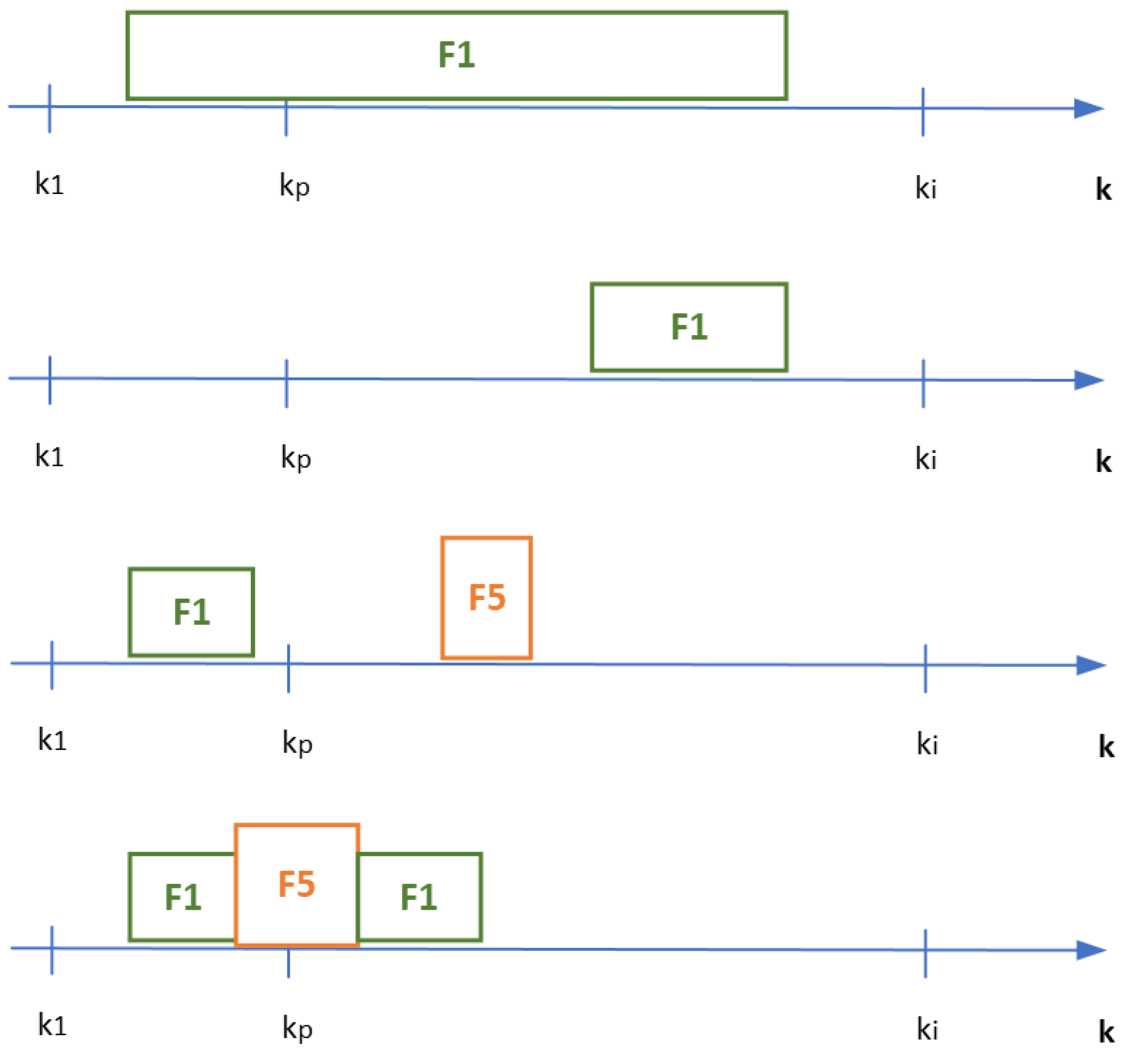
Fault identification occurs within a window w i = [ k 1 : k i ] of length n i , equivalent to three or four cycles (60 ms or 80 ms), where k 1 = t 1 / T s is associated with the fault detection time, as detailed in Figure 7. Applying the set of rules defined in Table 4 may result in the identification of one fault, two faults, or no fault (F0), given the transient behavior of short-circuit faults. In Figure 7, some possible faults identified in the window are depicted, where in this case the correct fault is fault F1.
In the probabilistic decision system proposed here (Figure 6), the fault identification window w i = [ k 1 : k i ] is divided in two sub-windows, w a = [ k 1 : k p ] and w b = [ k p + 1 : k i ] , assuming that K p = i n t ( K 1 + 1 / 4 × n i ) . In the case of identifying two faults in the window, during the simulations it was found that, in the vast majority of situations, the start of the correct fault occurs before the start of the incorrect fault, and typically within the first sub-window w a = [ k 1 : k p ] .
In this proposed fault identification approach, the decision regarding the correctly identified fault is based on the concept of the statistical mode (central tendency) of given datasets (sub-windows w a and w b ), as described next. Let us assume that the statistical mode M s (.) in sub-window w a is M a , and the statistical mode in sub-window w b is M b . It is necessary to deal with the situation where the statistical mode may result in fault F0 (no fault); the two conditions expressed in Equation (26) were established. Finally, the fault identified F i is obtained from Equation (27), given that the probability of the fault occurring in sub-window w a is greater than the probability of the fault occurring in sub-window w b .
First, the described fault identification algorithm is executed once considering that the window w i = [ k 1 : k i ] has a size equivalent to three cycles (60 ms). The simulations allowed us to conclude that the window size should be larger than the two cycles (40 ms) used in the Fourier and Hilbert transforms, also bearing in mind that some fault symptoms take longer to be revealed, possibly due to different fault locations.
i f ( M b = = F 0 ) t h e n M b = M a ; i f ( M a = = F 0 ) t h e n M a = M b ;
F i = M s ( [ M a M a M b ] )
As an example of application of the proposed fault identification approach, applying it to the case of Figure 7 results in the information presented in Table 7.
In summary, the tuning parameters of the fault identification algorithm presented in Equation (28) were obtained in order to (a) ensure tolerances in nominal operation associated with allowable load variations, since the typical allowable tolerances in voltage and current signals in nominal operation are, respectively, 5% and [10%; 20%]; and (b) minimize the cost function expressed by Equation (29) associated with high-impedance faults, subject to condition Equation (30), where N f = 619 is the number of CSV files processed.
[ G i , G u , n i ] = [ 1.2 , 0.95 , 3 or 4 cycles = 60 or 80 ms ]
J a = i = 1 N f F x ( i )
F x { F 1 , F 2 , F 3 , F 4 , F 5 , F 6 , F 7 }

3.5.2. Circuit Breaker Opening

For safety reasons, when a short-circuit fault is detected in any of the three phases (A, B, or C), the circuit breaker opens the power contacts associated with the three phases (A, B, and C). After fault detection at instant t 1 , detecting the instant in which the circuit breaker opens the power contacts is a relatively simple task, as the current in the power lines will tend to zero. Assuming t 2 > t 1 , this instant t 2 = t ( k ) is calculated when the condition described in Equation (31) is true for the first time in a sliding window of length N = 3 , using the current signals at time instants { k 2 ; k 1 ; k } , assuming some temporal redundancy in all the phases A, B, and C. The threshold H i x 2 should be a small value greater than zero, so the value H i x 2 = 1.0 was assumed.
( i 1 ( k ) < H i x 2 ) & & ( i 1 ( k 1 ) < H i x 2 ) & & ( i 1 ( k 2 ) < H i x 2 ) & & ( i 2 ( k ) < H i x 2 ) & & ( i 2 ( k 1 ) < H i x 2 ) & & ( i 2 ( k 2 ) < H i x 2 ) & & ( i 3 ( k ) < H i x 2 ) & & ( i 3 ( k 1 ) < H i x 2 ) & & ( i 3 ( k 2 ) < H i x 2 )

3.5.3. Circuit Breaker Closing

After the detection of the circuit breaker opening at instant t 2 , detecting the instant in which the circuit breaker closes the power contacts is a relatively simple task, as the current in the power lines will recover from zero to the nominal values. Assuming t 3 > t 2 , this instant t 3 = t ( k ) is calculated when the condition described in Equation (31) is true for the last time in a sliding window of length N = 3 , using the current signals at time instants { k 2 ; k 1 ; k } , assuming some temporal redundancy in all the phases: A, B, and C. The threshold H i x 2 should be a small value greater than zero, so the value H i x 2 = 1.0 was assumed.

3.5.4. Fault Recovery

Fault recovery corresponds to the situation in which the currents { i 1 , i 2 , i 3 } have frequencies close to the nominal value. After the detection of the circuit breaker closing at instant t 3 , detecting the instant of time t 4 = t ( k ) , assuming that t 4 > t 3 , in which the fault recovery occurs is a task with some complexity, as will be explained next. The main idea is to detect the instant t 4 in which the estimated instantaneous frequency of the current signals { i 1 , i 2 , i 3 } reaches a value close to the standard frequency; in Portugal, this value is 50 Hz ± 1 % , i.e., a range of [49.50; 50.50] Hz.
The estimation of the instantaneous frequency f i x ( . ) of current signals { i 1 , i 2 , i 3 } in a sliding window is carried out here using the discrete Hilbert transform (DHT). The Hilbert transform is useful in the analysis of nonstationary signals, in which the frequency may vary with time, expressing the frequency as a rate of phase variation [59].
Here, the instant t 4 = t ( k ) is calculated when the condition described in Equation (32) is true for the first time in a sliding window of length N = 400 , corresponding to one cycle (20 ms). In order to take into account the transient behavio r, it was established here that the estimated instantaneous frequency should belong to the range described in Equation (33), with d f = 15 Hz.
( ( m a x ( f i 1 ( k N + 1 : k ) ) f 50 + d f ) & & ( m i n ( f i 1 ( k N + 1 : k ) ) f 50 d f ) ) | | ( ( m a x ( f i 2 ( k N + 1 : k ) ) f 50 + d f ) & & ( m i n ( f i 2 ( k N + 1 : k ) ) f 50 d f ) ) | | ( ( m a x ( f i 3 ( k N + 1 : k ) ) f 50 + d f ) & & ( m i n ( f i 3 ( k N + 1 : k ) ) f 50 d f ) )
[ f 50 d f ; f 50 + d f ] = [ 50 Hz d f ; 50 Hz + d f ]

3.6. Thresholds and Robustness to Noise

As mentioned in Section 3.2, in this work, in order to emulate some of the situations referred to as load imbalances, load variations, and voltage distortions, Gaussian noise was added to the voltage and current signals, assuming different signal-to-noise ratios (SNRs). Table 8 summarizes all thresholds used in this work, described earlier in Section 3. The proposed FDD approach is robust to noise since the thresholds are adaptive, and depend on the SNR computed in the nominal operating region.

3.7. Pseudo-Code of the Hybrid FDD Algorithm

In order to clarify and explain in a sequential way the proposed FDD approach, the pseudo-code of the implemented algorithm is presented next, in Algorithm 1.
The algorithms were programmed in the Python language using classes and objects. In some lines, comments are presented at the end, referring to the subsections where the various tasks are described; for example, “S:3.2” refers to Section 3.2.
Algorithm 1 Hybrid Fault Detection and Diagnosis
1:
Class Signals; Sig = Signals(.);                              {/* Python Class + Object */}
2:
Class RENSignals; SRen = RENSignals(.);                {/* Python Class + Object */}
3:
NumFiles = 619;                                                      {/* 619 CSV files */}
4:
for  i = 1 to N u m F i l e s  do
5:
   [U1,U2,U3,U0,I1,I2,I3,I0] = Load_Signals_from_CSV_File(SRen,i);
6:
   Sig.Ux = [U1,U2,U3,U0]; Sig.Ix = [I1,I2,I3,I0];
7:
   for  k = 1 to n do
8:
     Sig = Add_Noise_Evaluate_SNR(Sig);                                      {S: 3.2}
9:
     Sig.t0 = Fault_Start(Sig,Sig.i0);                                  {Fault_start, S: 3.2}
10:
     [U1n,U2n,U3n,U0n] = Capture_Nominal_Data(Sig.Ux,Sig.t0);             {S: 3.4}
11:
     Sig.Un = [U1n,U2n,U3n,U0n];
12:
     [Sig.H] = Compute_Thresholds(Sig);                              {Table 8, S: 3.6}
13:
     [P,T1,T2] = Compute_2D_Nominal_PCA_Model(Sig.Un);                    {S: 3.4}
14:
     [T1f,T2f] = Project_Data_using_PCA_Model(Sig.Ux,P);                    {S: 3.4}
15:
     [Sig.Re] = Compute_Fault_Detection_Residual(T1f,T2f,T1,T2);             {S: 3.4}
16:
     if (Sig.Re(k) > Sig . H R e (k)) then
17:
             Sig.t1 = t(k); Fde = 1;                                  {Fault detected, S: 3.4}
18:
     end
19:
     [Ae_Ux,Ae_Ix] = SW_Disc_Fourier_Transform(Sig);                       {S: 3.5}
20:
     [Sig.ti,Sig.fault] = Fault_Identif(Sig,Ae_Ux,Ae_Ix,Sig.t1);   {Fault identified, S: 3.5}
21:
     [Sig.t2] = CBreaker_Opening_Detection(Sig,Sig.t1);         {CB Opening, S: 3.5}
22:
     [Sig.t3] = CBreaker_Closing_Detection(Sig,Sig.t2);             {CB Closing, S: 3.5}
23:
     [Fe_Ix] = SW_Hilbert_Transform(Sig,Sig.t3);                                  {S: 3.5}
24:
     [Sig.t4] = Fault_Recovering_Detec(Sig,Sig.t3,Fe_Ix);      {Fault recovering, S: 3.5}
25:
     Fault_detection_delay = Sig.t1 - Sig.t0;
26:
     Fault_identification_delay = Sig.ti - Sig.t1;
27:
     CB_actuation_delay = Sig.t2 - Sig.t0;
28:
     CB_reconnection_time = Sig.t4 - Sig.t2;
29:
     Save_Results(“bd4nrg.txt”,“append”);
30:
   end for
31:
end for

4. Simulation Results and Discussion

In this section, most of the simulation results presented in the figures are related to short-circuit fault “ABG” (F6), associated with the first file “LCGRM1_1_11_15_54.csv” of the big dataset. In some figures, some simulation results related to short-circuit fault F1 (CG), associated with the last file “LCGRM1_7_20_24_10.csv” of the big dataset, are also presented. Both simulations were performed with signal-to-noise ratios of SNR i = 30 dB and SNR u = 35 dB.
Here, a discussion is provided regarding the performance of the new proposed FDD approach. A performance comparison of the proposed FDD approach with other FDD approaches (rule-based and ML/AI-based) is also provided.

4.1. Dataset, HyperSim, and Programming Language

As mentioned in Section 3.1, a big dataset with synthetic data comprising 619 CSV files was created by the REN company using the HyperSim simulator, containing the seven typical short-circuit faults described in Table 4. Each CSV file was saved in a different directory. The 619 directories occupy 2.87 gigabytes of disk space. In the near future, this big dataset, with 619 CSV files, should be available in open access (e.g., in OpenAIRE—https://www.openaire.eu (accessed on 28 March 2024)). The big dataset allowed for around 90 files for each type of short-circuit fault, facilitating the testing of the algorithms and the tuning of their parameters, as well as their validation.
In Table 9, the HyperSim simulator parameters used to generate the big dataset can be observed. HyperSim allows a diversity of topological and operational scenarios of the electrical network to be simulated, i.e., variation in the fault resistance, variation in the location where the fault occurred along the power transmission lines, and also the different moments for each of the events (start of fault, end of fault, circuit breaker opening and closing), for models of 12 overhead power lines in Portugal with different voltages (150 kV, 220 kV, and 400 kV) [46].
The developed FDD algorithms were implemented in the Python programming language (v3.8), https://www.python.org/ (accessed on 28 March 2024) [60,61], on a computer with Windows 64 bits OS, 32 GB of RAM and Intel(R) Core(TM) i7-6700K CPU @ 4.00 GHz 4.00 GHz processor. The CPU processing time for each CSV file was around 58 s, given that the Python language is interpreted, and also there was no concern about optimizing some routines that included some graphics. It may be possible to reduce this time to a few seconds using faster hardware, a compiled language, and optimization routines.
In each simulation performed in the HyperSim simulator, the simulation time t m a x was 1.5 s. Given that the sampling time used was T s = 50 µs, the number of samples in each current signal and voltage signal was n = 30,001. Considering the standard frequency f 50 = 50 Hz, which corresponds to a period of T = 20 ms, each cycle (period) had 400 samples associated.
In Table 10, the seven short-circuit faults considered in this work, and also some filename examples, are presented.

4.2. Simulation Parameters

In order to facilitate understanding of the work, in Table 11, the main simulation parameters and times are presented. It should be highlighted that the proposed FDD approach was tested with a big dataset that considers situations of noise, different signal-to-noise ratios, load variations, and low-, medium-, and high-impedance short-circuit faults.

4.3. Fault Detection Results

The fault detection simulation results with fault F6 (ABG) and fault F1 (CG) are presented and analyzed, considering SNR i = 30 dB and SNR u = 35 dB. For other types of short-circuit faults, the performance was similar.
In Figure 8, the added noise, and current and voltage signals with added noise, in the nominal operating region ([0.0; 0.10] s), can be observed. From top to bottom, the following signals can be observed: (a) noise added to voltage u 1 ; (b) voltage u 1 with noise, where SNR u = 35 dB; (c) noise added to current i 1 ; (d) current i 1 with noise, where SNR i = 30 dB; (e) current i 0 , which verifies the condition | i 0 ( k ) | < 1 described in Equation (3).
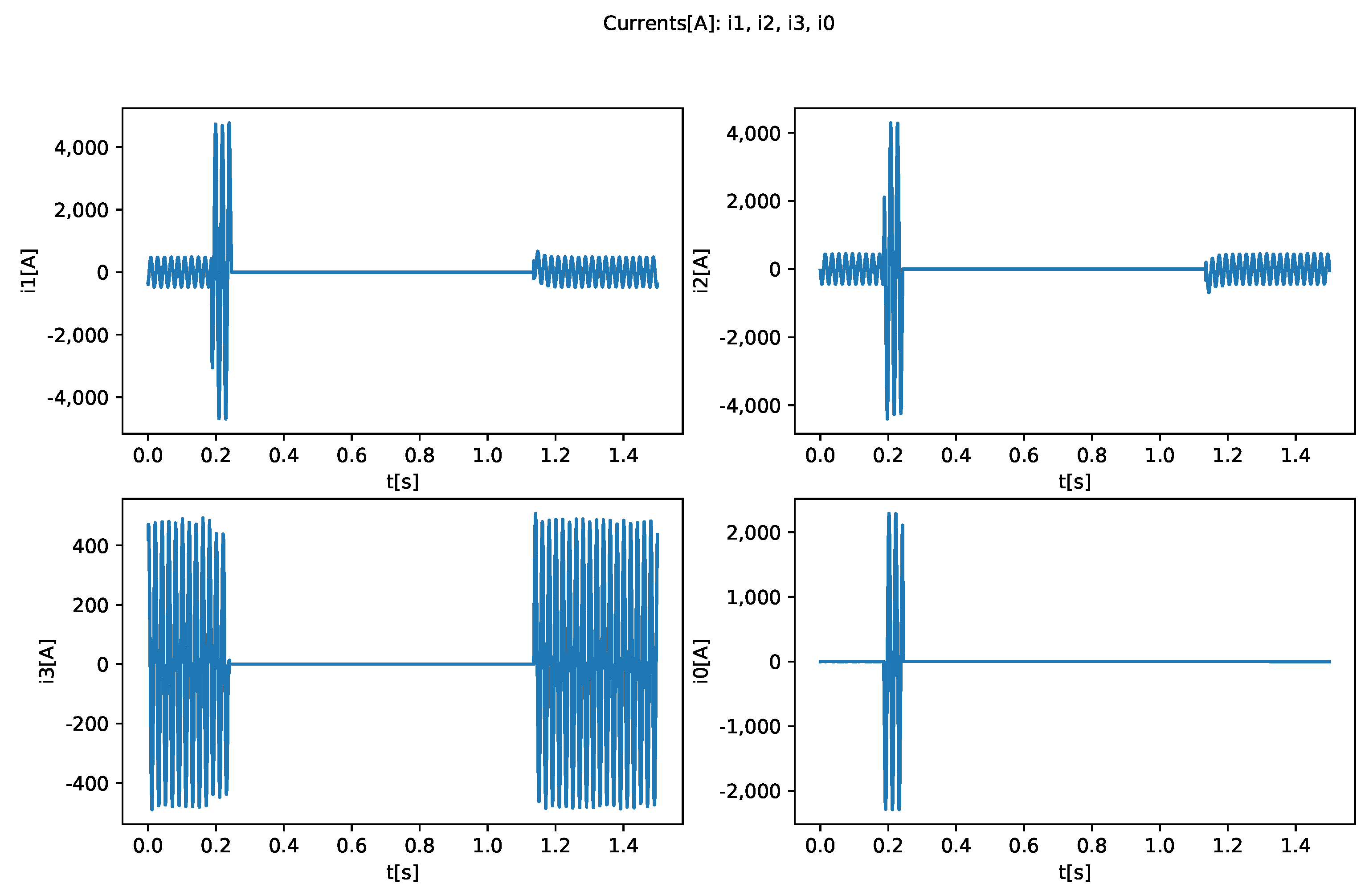
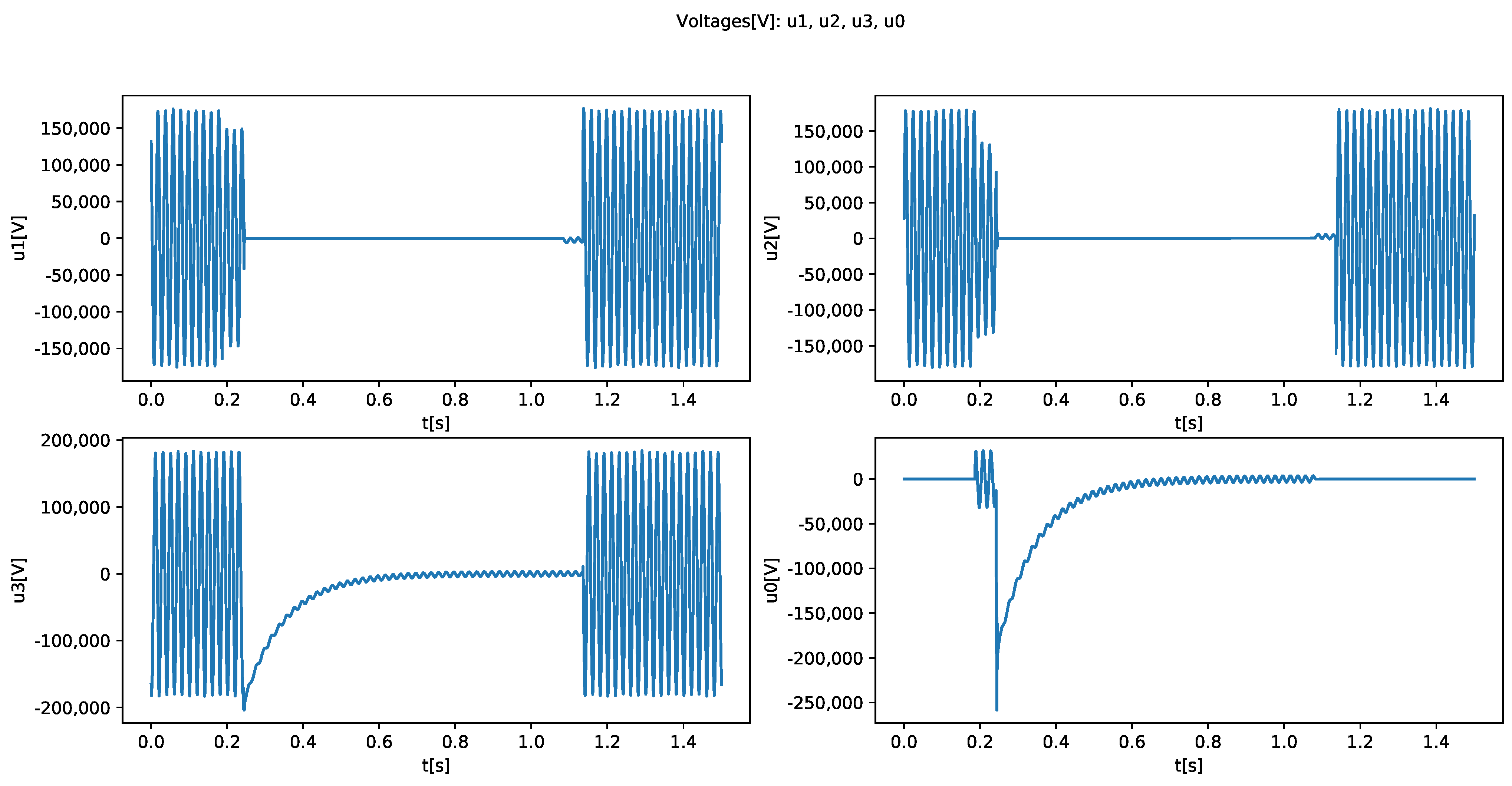
For fault F6 (ABG), two main symptoms are expected: a rapid increase in current signals [ i 1 i 2 ] and a rapid decrease in voltage signals [ u 1 u 2 ] . In Figure 9 and Figure 10, respectively, in the instant t ( k ) = 0.187 s, which corresponds to sample k = 3740 , these two main symptoms can be observed. In phase A, the amplitude of the current i 1 quickly changed from a value close to 460 A to 4700 A, and the amplitude of the voltage u 1 quickly changed from a value close to 170,000 V to 145,000 V. In phase B, the amplitude of the current i 2 quickly changed from a value close to 450 A to 4300 A, and the amplitude of the voltage u 2 quickly changed from a value close to 180,000 V to 130,000 V. In phase C, variations in current and voltage amplitudes are of little significance.
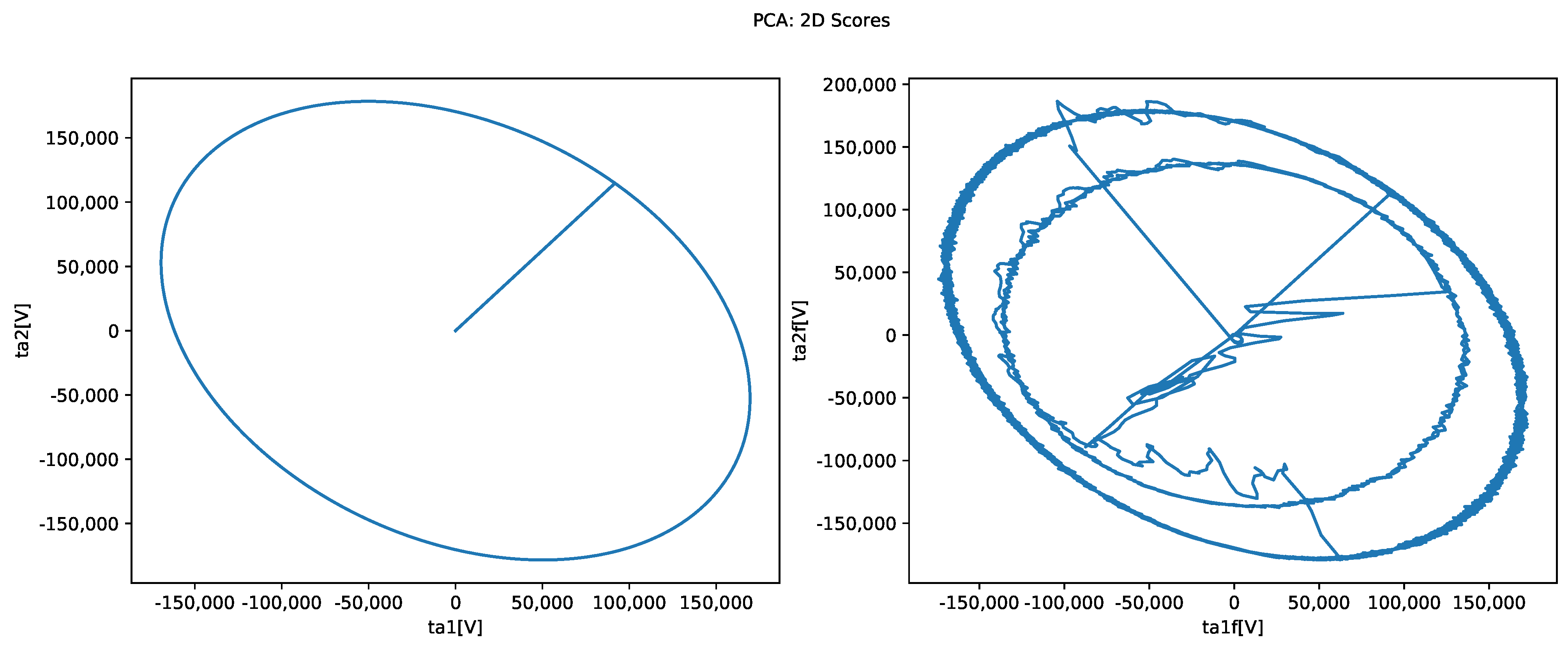
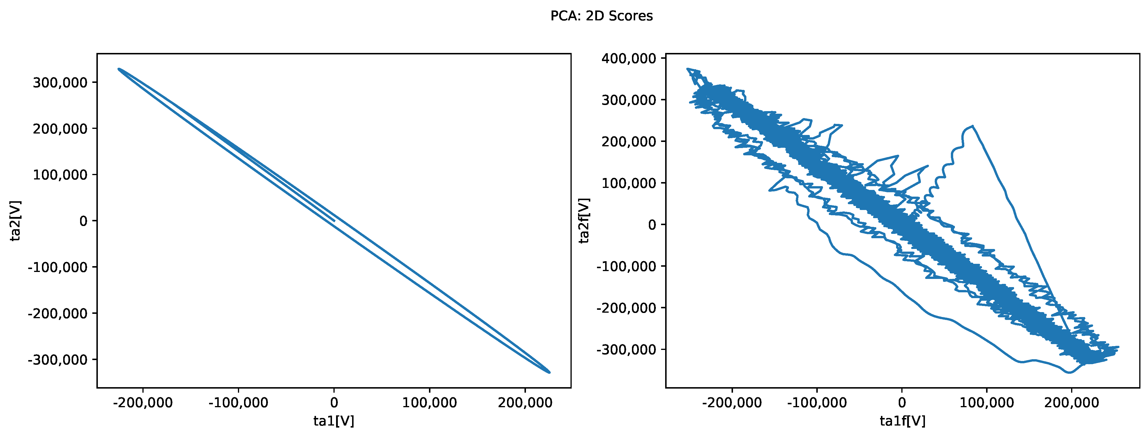
In Figure 11, the PCA 2D scores are presented, for nominal behavior without a fault (left panel) and for behavior with a fault (right panel). When the fault occurs, the scores moves away from the ellipse (nominal PCA model) as the correlation between the voltage signals [ u 1 u 2 u 3 u 0 ] changes. In Figure 12, now the PCA 2D scores for fault F1 (CG) are presented, for nominal behavior without a fault (left panel) and for behavior with a fault (right panel).
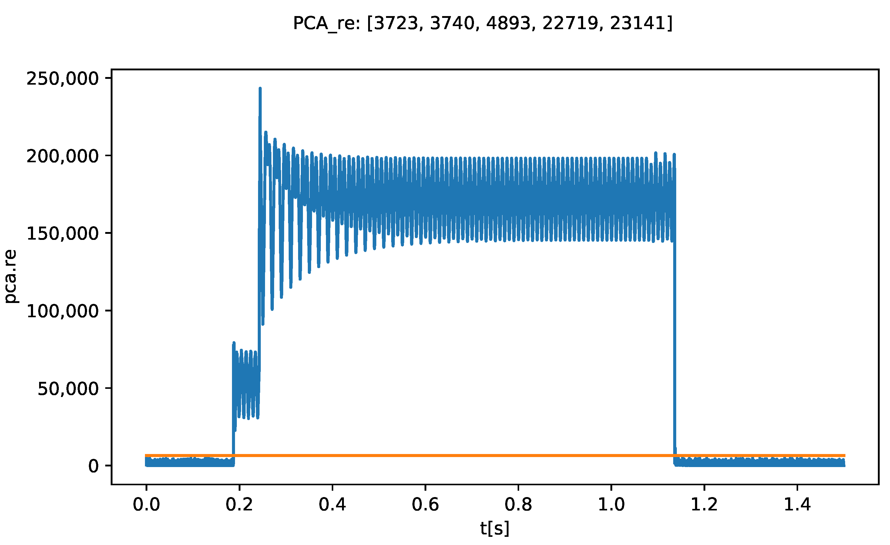
The proposed fault detection approach detects the short-circuit fault based on the R e ( k ) signal described in Equation (17), as can be observed in Figure 13. The R e ( k ) signal is drawn in blue, and the adaptive threshold H R e ( k ) described in Equation (21) is drawn in orange; the short-circuit fault is detected when the R e ( k ) signal exceeds the threshold H R e ( k ) . In the figure title, the vector associated with the fault times [ t 0 , t 1 , t 2 , t 3 , t 4 ] , in samples [ 3723 , 3740 , 4893 , 22719 , 23141 ] , is presented.
The simulation results obtained with the proposed fault detection approach are in line with expectations, and in the future the performance could be improved.

4.4. Fault Diagnosis Results

In this section, the fault diagnosis simulation results with short-circuit faults F6 (ABG) and F1 (CG) are presented and analyzed. For other types of short-circuit faults, the performance was similar.
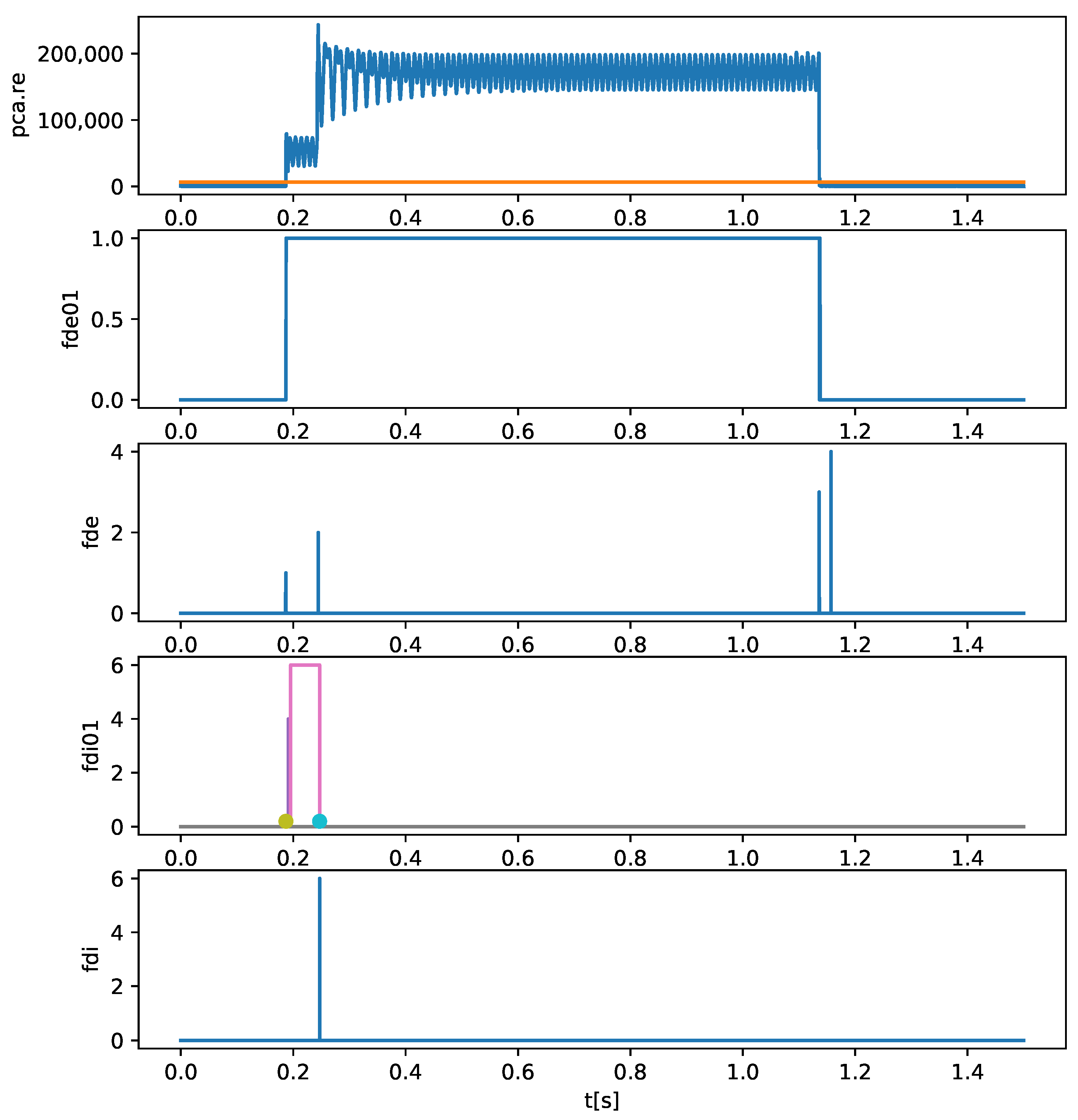
In Figure 14, in the graphics presented, from top to bottom, the following signals can be observed for fault F6 (ABG):
  • (a) the fault detection signal “Re” (blue signal), and the respective adaptive threshold (orange signal);
  • (b) the signal “fde01”, which corresponds to the moments in which the fault is active;
  • (c) the “fde” signal, that records the various time instants, [ t 0 t 1 t 2 t 3 t 4 ] ; In the figure title, the vector associated with the fault times [ t 0 , t 1 , t 2 , t 3 , t 4 ] , in samples [ 3723 , 3740 , 4893 , 22719 , 23141 ] , is presented.
  • (d) the “fdi01” signal, that allows evaluating, in the identification window, the short-circuit faults identified; in this case, two faults were identified: first, the fault F4 (AG) for a short time (in magenta color); and second, the correct fault F6 (ABG) for most of the time (in pink color);
  • (e) the signal “fdi”, which indicates which fault was well identified based on the rules and on the probabilistic decision system: in this case, fault F6 (ABG) and the respective instant t i ; the colored dots define the beginning and end of the fault identification window;
  • (f) the relevant FDD times are [ t 0 t 1 t 2 t 3 t 4 ] = [ 0.186 0.187 0.245 1.136 1.157 ] s, and t i = 0.247 s;
  • (g) the title of the figure also mentions the number of the processed file (0, in this case), the identified fault "ABG" and the real fault "ABG*" (marked with the symbol "*").
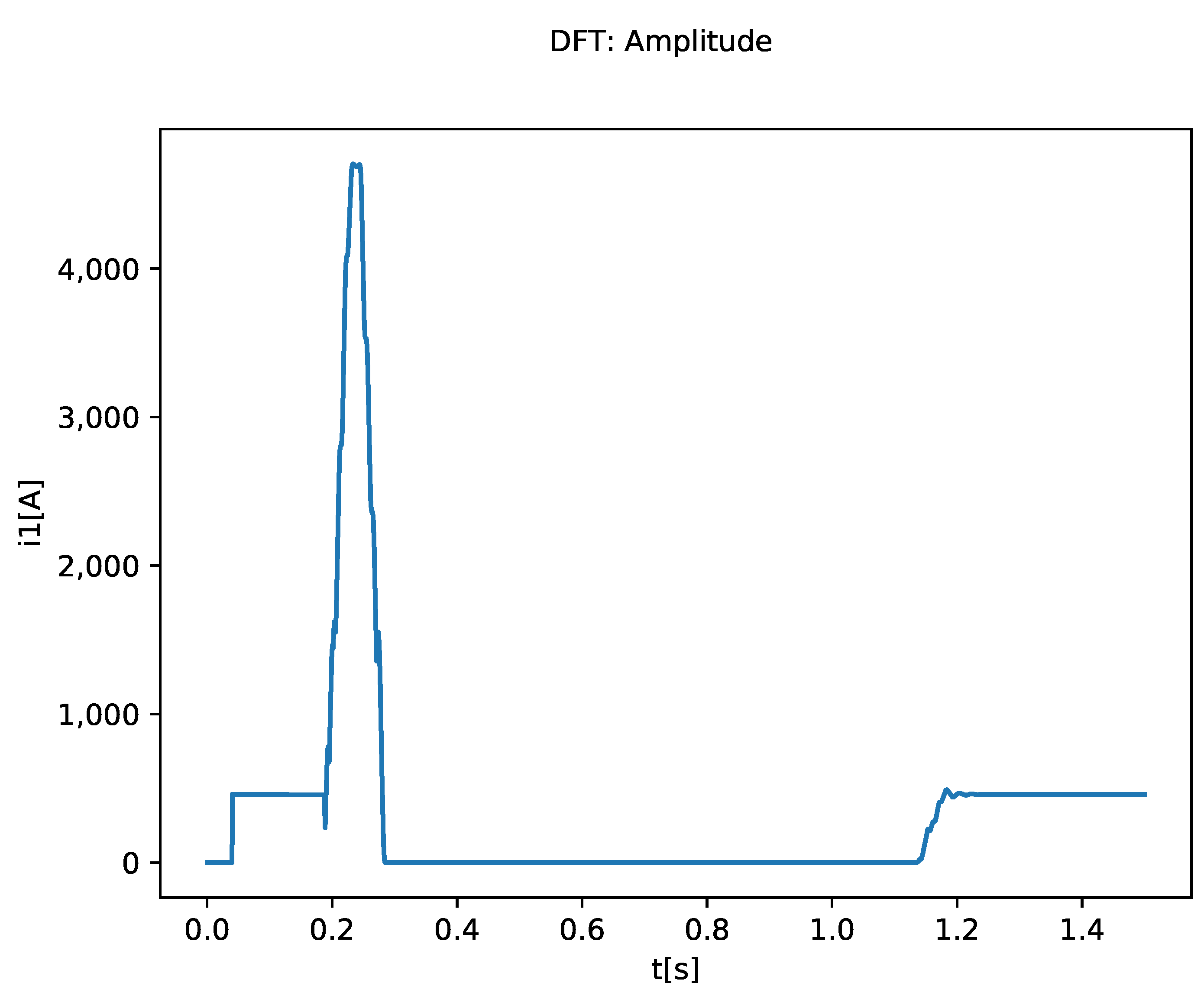
In order to elucidate the dynamic behavior of the amplitudes estimated by discrete Fourier transform (DFT), in Figure 15, for fault F6 (ABG), a graphic with the estimation of the amplitude of the current i 1 using the DFT, based on a sliding window algorithm, is depicted. Estimation of current and voltage amplitudes is necessary to implement the fault identification task.
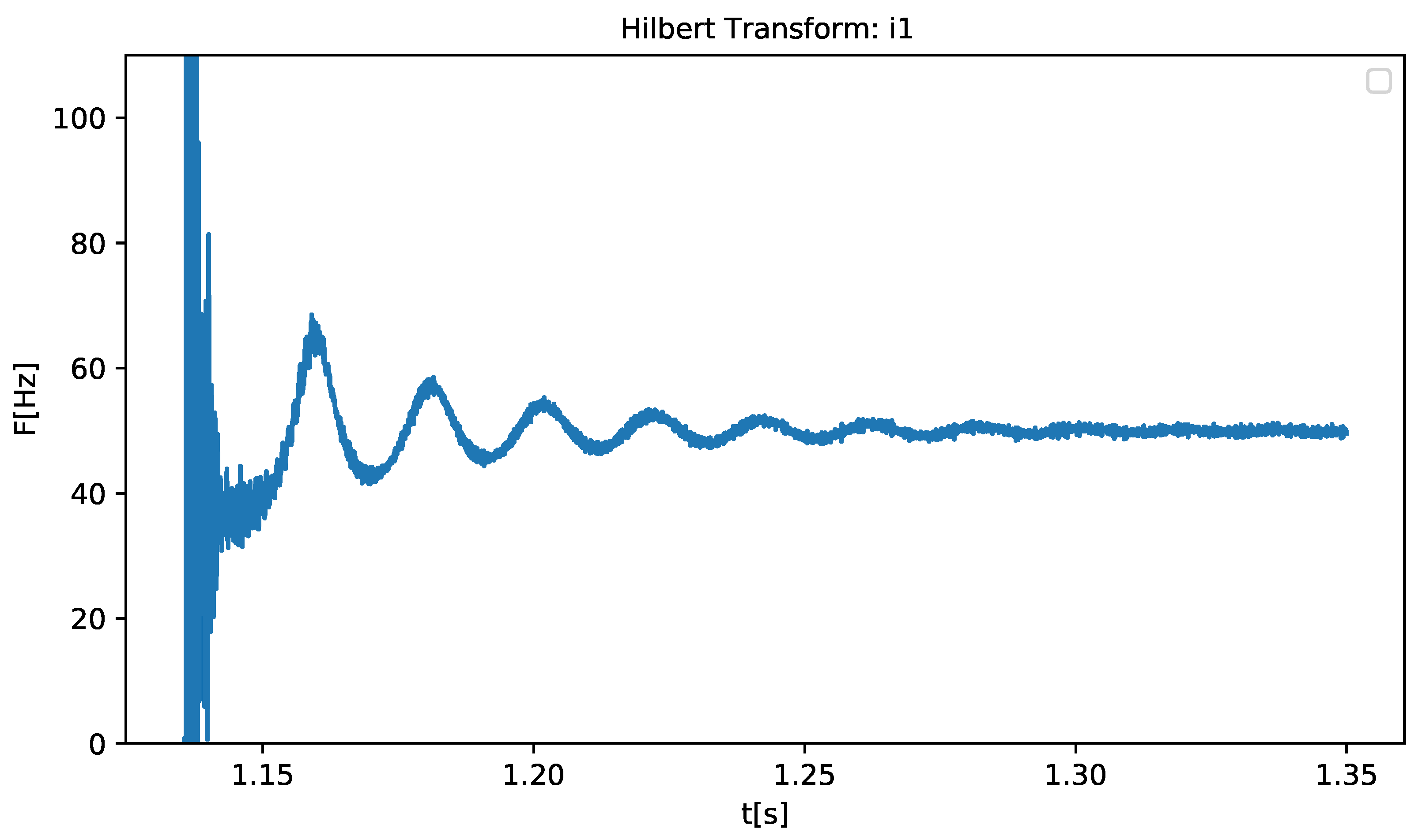
In order to elucidate the dynamic behavior of the frequencies estimated by discrete Hilbert transform (DHT), in Figure 16, for fault F6 (ABG), a graphic with the estimation of the instantaneous frequency of the current i 1 using the discrete Hilbert transform, based on a sliding window algorithm, is depicted. The Hilbert transform allowed us to determine the instant t 4 associated with fault recovery. It can be observed that after circuit breaker reclosing, the frequency of current i 1 tends to 50 Hz, as expected.
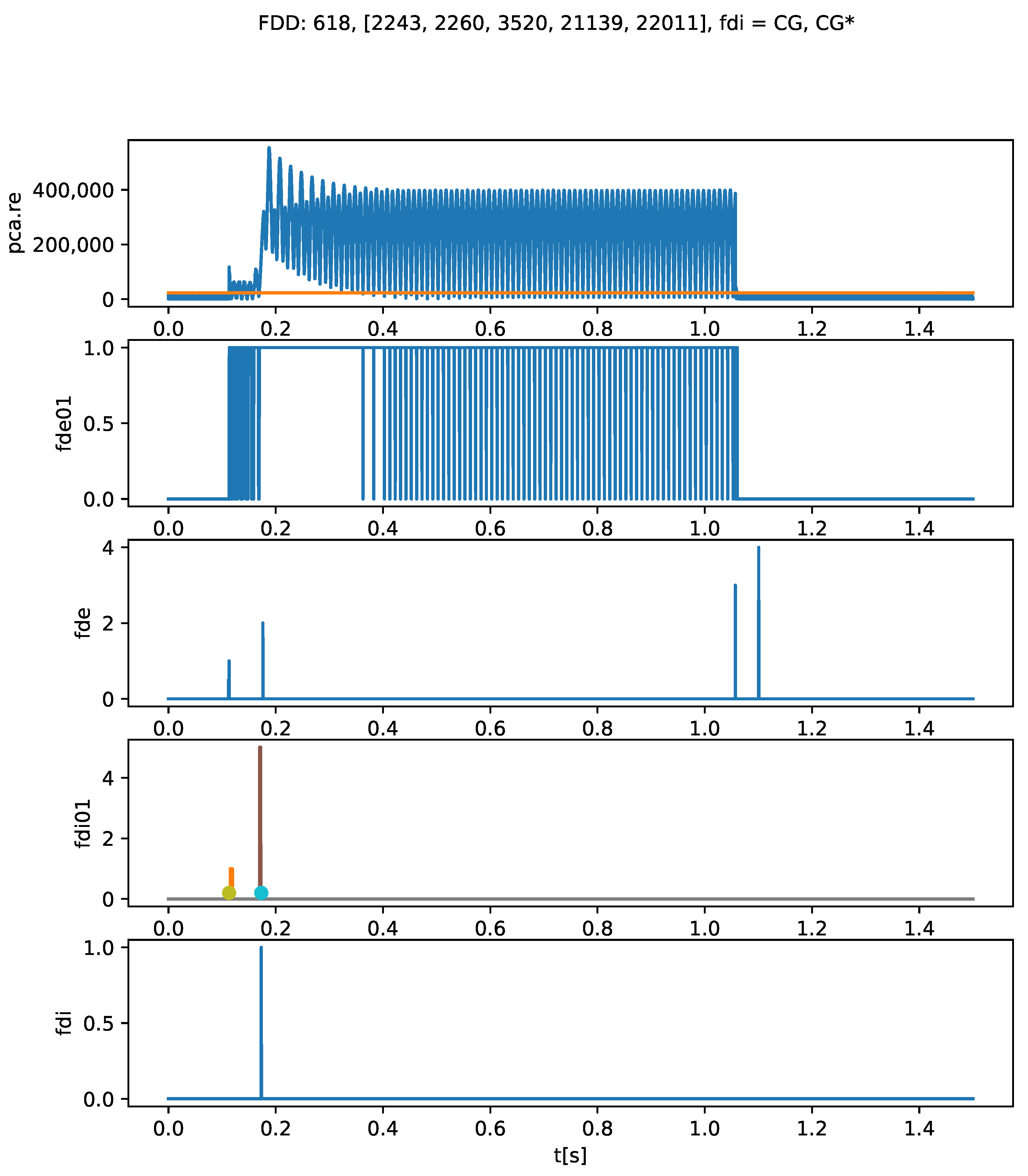
In Figure 17, in the graphics presented, from top to bottom, the following signals can be observed for fault F1 (CG):
  • (a) the fault detection signal “Re” (blue signal), and the respective adaptive threshold (orange signal);
  • (b) the signal “fde01”, which corresponds to the moments in which the fault is active;
  • (c) the “fde” signal, that records the various time instants, [ t 0 t 1 t 2 t 3 t 4 ] ; In the figure title, the vector associated with the fault times [ t 0 , t 1 , t 2 , t 3 , t 4 ] , in samples [ 2243 , 2260 , 3520 , 21139 , 22011 ] is presented.
  • (d) the “fdi01” signal, that allows evaluation of, in the identification window, the short-circuit faults identified; in this case, two faults were identified: first, the correct fault F1 (CG) at the beginning of the identification window (in orange color); and second, the fault F5 (ACG) at the end of the identification window (in brown color);
  • (e) the signal “fdi”, which indicates which fault was well identified based on the rules and on the probabilistic decision system: in this case fault F1 (CG) and the respective instant t i ; the colored dots define the beginning and end of the fault identification window;
  • (f) the relevant FDD times are [ t 0 t 1 t 2 t 3 t 4 ] = [ 0.112 0.113 0.176 1.057 1.101 ] s, and t i = 0.173 s;
  • (g) the title of the figure also mentions the number of the processed file (618, in this case), the identified fault "CG" and the real fault "CG*" (marked with the symbol "*").

4.5. Main Results and Discussion

To allow conclusions to be made about the overall performance, in Table 12 the main simulation results, without noise, for all the 619 CSV files processed, are presented. The pseudo-fault Fx (xyz) is associated with the faults that were not identified, as a typical fault belongs to the set {F1; F2; F3; F4; F5; F6; F7}; these are high-impedance faults, which cause a small increase in the short-circuit current, and for this reason they are difficult to identify given the thresholds used. Note that all short-circuit faults were detected by the proposed approach. For each fault, the number of faults generated by the HyperSim simulator (“Sim”), the number of well-identified faults (“FDD”), and the difference between previous values (“FDD-Sim”), are presented. The last line of the table provides validation of the values.
The information available in Table 13, FDD main simulation results for different SNR i , allows Table 14 to be built; the “Sim” column indicates the real number of faults, and the “FDD” column indicates the number of faults identified by the FDD approach. In Table 14, the main global performance indices ( η ) are presented. The fault detection performance is 100%, for any SNR. The fault identification performance has a value in the range [97.09; 98.22]%, depending on SNR; the best performance (98.22%) occurs for SNR = 30 dB, given that the probabilistic decision system was tuned for this central SNR value. These fault detection and identification results reveal that the proposed FDD approach presents good robustness to noise.
As fault detection and diagnosis systems implemented in hardware/software may perform at less than 100%, when a fault is detected in any of the three phases (A, B, or C), for safety reasons the circuit breaker opens all the power contacts associated with the three phases (A, B, and C).
In Table 15, for the circuit breakers, the mean values and the standard deviations of actuation delay and reconnection time are presented. The mean value of the reconnection time is close to the typical value for circuit breakers, which is around 0.90 s, as mentioned in Table 9. The mean value of the actuation delay is similar to values obtained with other approaches, such as Ref. [44]. The fault detection delay depends on the SNR, and takes mean values in the range [0.80; 4.83] ms; these mean values are less than 17 ms, a value obtained in Ref. [44]. The mean value of the fault identification delay is closer to the mean value of the circuit breaker actuation delay, assuming an approximate value of 60 ms.
In Table 16, the proposed FDD approach is compared to other studies in the literature, in terms of fault identification accuracy/performance, η [ % ] . The “dataset” column shows the type of dataset/software used. The “noise” column indicates which references considered noise in the tests carried out. The proposed robust rule-based FDD approach achieved very high performance, similar to the performances of machine learning/artificial intelligence (ML/AI) approaches, validating this FDD approach. It is important to highlight that the rule-based hybrid FDD approach proposed in this work, considering noise, achieved similar performance to the ML/AI approach [46] based on wavelet transform and neural networks, without considering noise, using the same big dataset (REN: HyperSim).
High-impedance faults are very difficult to detect and diagnose using traditional monitoring equipment because their presence results in only a slight increase in load currents and a slight decrease in load voltages. More research should be performed on the topic of FDD of high-impedance faults. A methodology with the potential to solve this type of incipient fault could be the use of deep learning approaches, such as nonlinear Deep-PCA [62].

5. Conclusions

The proposed rule-based hybrid fault detection and diagnosis approach, developed in the context of the H2020 BD4NRG EU Project—Big Data for Next Generation Energy, implemented in Python, allows the detection and diagnosis of short-circuit faults in power transmission lines, and it can be applied to high-/medium-voltage power transmission lines as well to low-voltage electronic transmission systems.
This hybrid FDD approach, combining different classical approaches such as PCA, DFT, DHT and probabilistic decision, without resorting to optimization techniques, takes advantage of the potential of each approach, with the aim of obtaining high accuracy in identifying faults (around 98%), similar to the performances of ML/AI-based approaches. The proposed FDD approach was tested and validated on a big dataset (619 files), having achieved 100% accuracy in detecting short-circuit faults, as detailed in Table 14.
The use of adaptive thresholds allowed situations of load imbalances, load variations, and voltage distortions, to be dealt with, modeled as different signal-to-noise ratios (SNRs), revealing the good robustness to noise of the proposed FDD approach. Adaptive thresholds also made it possible to better deal with various fault situations, such as low-, medium-, and high-impedance short-circuit faults.
The proposed robust FDD approach can be used to evaluate the stress to which the circuit breakers are subjected, providing information to supervision- and condition-based monitoring systems, in order to improve predictive and preventive maintenance strategies.
Some pointers for future work are (a) improve the performance of the proposed FDD approach using optimization techniques, to compute tuning parameters and thresholds; (b) estimate the short-circuit fault resistance; (c) develop an FDD approach to deal better with high-impedance faults based on nonlinear deep-PCA; (d) better compare this robust FDD approach with other FDD approaches, for the same big dataset, such as ML/AI approaches.

Funding

This research was funded by H2020 BD4NRG European Project—GA872613, grant agreement no. 872613, https://www.bd4nrg.eu/ (accessed on 18 March 2024). The APC was funded by the H2020 BD4NRG European Project and by the UNINOVA research institute (https://www.uninova.pt(accessed on 28 March 2024)).

Data Availability Statement

In the near future, this big dataset, with 619 CSV files, should be available in open access.

Acknowledgments

This work has been supported by H2020 BD4NRG European Project—GA872613, https://www.bd4nrg.eu/ (accessed on 18 March 2024), by Department of Electrical and Computer Engineering of NOVA School of Science and Technology (FCT NOVA), by CTS-UNINOVA and LASI research units, and by national funds through FCT-Fundação para a Ciência e a Tecnologia within the Research unit CTS—Centro de Tecnologia e Sistemas—UIDB/00066/2020. The authors would like to thank all the institutions, and also thank the REN company and the R&D Nester ID center, for the simulation data made available and for the exchange of knowledge. Colleagues Pedro Maló, Rui Azevedo Antunes and Paulo Gil deserve thanks for their support in some phases of the H2020 BD4NRG European Project.

Conflicts of Interest

The authors declare no conflicts of interest.

Abbreviations

The following abbreviations are used in this manuscript:
ACDActuation delay of circuit breaker, t 2 t 0
AIArtificial intelligence
CBCircuit breaker
CBCCircuit breaker closing, t 3
CBOCircuit breaker opening, t 2
DFTDiscrete Fourier transform
DHTDiscrete Hilbert transform
EWTEmpirical wavelet transform
FAIFault identification, t i
FARFault recovery, t 4
FASFault start, t 0
FDDFault detection and diagnosis
FDEFault detection, t 1
HIFHigh-impedance faults
MLMachine learning
PCAPrincipal component analysis
RETReconnection time of circuit breaker, t 4 t 2
SNRSignal-to-noise ratio
SVDSingular value decomposition
SVMSupport vector machine

References

  1. Kiessling, F.; Nefzger, P.; Nolasco, J.; Kaintzyk, U. Overhead Power Lines: Planning, Design, Construction; Springer: Berlin/Heidelberg, Germany, 2003. [Google Scholar]
  2. Conejo, A.; Baringo, L. Power System Operations; Springer: Cham, Switzerland, 2017. [Google Scholar]
  3. Kothari, D.; Nagrath, I. Modern Power System Analysis; Tata McGraw-Hill: New Delhi, India, 2011. [Google Scholar]
  4. Das, J. Short-Circuits in AC and DC Systems: ANSI, IEEE, and IEC Standards (Power Systems Handbook); CRC Press: Boca Raton, FL, USA, 2018. [Google Scholar]
  5. Flurscheim, C. Power Circuit Breaker Theory and Design; IEE Power Engineering Series 1; Peter Peregrinus Ltd.: London, UK, 1982. [Google Scholar]
  6. Ciufo, J.; Cooperberg, A. Power System Protection—Fundamentals and Applications; Wiley: Hoboken, NJ, USA; IEEE Press: Piscataway, NJ, USA, 2021. [Google Scholar]
  7. Anderson, P.; Henville, C.; Rifaat, R.; Johnson, B.; Meliopoulos, S. Power System Protection; Wiley: Hoboken, NJ, USA; IEEE Press: Piscataway, NJ, USA, 2021. [Google Scholar]
  8. Papailiou, K. (Ed.) Springer Handbook of Power Systems; Springer: Gateway East, Singapore, 2021. [Google Scholar]
  9. Abood, S.; Fuller, J. Power System Protection and Relaying—Computer-Aided Design Using SCADA Technology; CRC Press: Boca Raton, FL, USA, 2023. [Google Scholar]
  10. Brito Palma, L. Fault Detection, Diagnosis and Fault Tolerance Approaches in Dynamic Systems based on Black-Box Models. Ph.D. Thesis, NOVA University Lisbon, Lisbon, Portugal, 2007. Available online: https://run.unl.pt/handle/10362/66049 (accessed on 8 February 2024).
  11. Blanke, M.; Kinnaert, M.; Lunze, J.; Staroswiecki, M. Diagnosis and Fault-Tolerant Control; Springer: Berlin/Heidelberg, Germany, 2010. [Google Scholar]
  12. Ding, S. Advanced Methods for Fault Diagnosis and Fault-Tolerant Control; Springer: Berlin/Heidelberg, Germany, 2021. [Google Scholar]
  13. Bindi, M.; Piccirilli, M.; Luchetta, A.; Grasso, F. A Comprehensive Review of Fault Diagnosis and Prognosis Techniques in High Voltage and Medium Voltage Electrical Power Lines. Energies 2023, 16, 7317. [Google Scholar] [CrossRef]
  14. Raza, A.; Benrabah, A.; Alquthami, T.; Akmal, M. A Review of Fault Diagnosing Methods in Power Transmission Systems. Appl. Sci. 2020, 10, 1312. [Google Scholar] [CrossRef]
  15. Furse, C.; Kafal, M.; Razzaghi, R.; Shin, Y. Fault Diagnosis for Electrical Systems and Power Networks: A Review. IEEE Sens. J. 2021, 21, 888–906. [Google Scholar] [CrossRef]
  16. Nandhini, K.; Prajith, C. Review on Fault Detection and Classification in Transmission Line using Machine Learning Methods. In Proceedings of the 5th International Conference on Control, Communication and Computing (ICCC), Kerala, India, 19–21 May 2023. [Google Scholar]
  17. Park, Y.; Fan, S.; Hsu, C. A Review on Fault Detection and Process Diagnostics in Industrial Processes. Processes 2020, 8, 1123. [Google Scholar] [CrossRef]
  18. Rezapour, H.; Jamali, S.; Bahmanyar, A. Review on Artificial Intelligence-Based Fault Location Methods in Power Distribution Networks. Energies 2023, 16, 4636. [Google Scholar] [CrossRef]
  19. Shakiba, F.; Azizi, S.; Zhou, M.; Abusorrah, A. Application of Machine Learning Methods in Fault Detection and Classification of Power Transmission Lines: A Survey. Artif. Intell. Rev. 2023, 56, 5799–5836. [Google Scholar] [CrossRef]
  20. Isermann, R.; Ballé, P. Trends in the Application of Model-Based Fault Detection and Diagnosis of Technical Processes. Control Eng. Pract. 1997, 5, 709–719. [Google Scholar] [CrossRef]
  21. Isermann, R. Fault Diagnosis Systems; Springer: Berlin/Heidelberg, Germany, 2006. [Google Scholar]
  22. Fleckenstein, J. Three-Phase Electrical Power; CRC Press: Boca Raton, FL, USA, 2016. [Google Scholar]
  23. Grigsby, L. Electric Power Generation, Transmission, and Distribution; CRC Press: Boca Raton, FL, USA, 2012. [Google Scholar]
  24. Chattopadhyay, S.; Das, A. Overhead Electric Power Lines: Theory and Practice; The Institution of Engineering and Technology (IET): Stevenage, UK, 2021. [Google Scholar]
  25. Wang, X.; Hu, H.; Liang, Z.; Guo, L.; Gao, J.; Kheshti, M.; Liu, W. Single Phase to Ground Fault Location Method of Overhead Line based on Magnetic Field Detection and Multi-Criteria Fusion. Int. J. Electr. Power Energy Syst. 2023, 145, 108699. [Google Scholar] [CrossRef]
  26. Gonen, T. Modern Power System Analysis; CRC Press: Boca Raton, FL, USA, 2016. [Google Scholar]
  27. Ibrahim, M. Disturbance Analysis for Power Systems; Wiley: Hoboken, NJ, USA, 2012. [Google Scholar]
  28. Saha, M.; Izykowski, J.; Rosolowski, E. Fault Location on Power Networks; Springer: Berlin/Heidelberg, Germany, 2010. [Google Scholar]
  29. Dashtdar, M.; Hussain, A.; Al Garni, H.Z.; Mas’ud, A.A.; Haider, W.; AboRas, K.M.; Kotb, H. Fault Location in Distribution Network by Solving the Optimization Problem Based on Power System Status Estimation Using the PMU. Machines 2023, 11, 109. [Google Scholar] [CrossRef]
  30. Haydaroglu, C.; Gumus, B. Fault Detection in Distribution Network with the Cauchy-M Estimate—RVFLN Method. Energies 2023, 16, 252. [Google Scholar] [CrossRef]
  31. Short, T. Electric Power Distribution Equipment and Systems; CRC Press: Boca Raton, FL, USA, 2019. [Google Scholar]
  32. Das, J. Power Systems Protective Relaying (Power Systems Handbook); CRC Press: Boca Raton, FL, USA, 2018. [Google Scholar]
  33. Gertler, J. Fault Detection and Diagnosis in Engineering Systems; CRC Press: Boca Raton, FL, USA, 2017. [Google Scholar]
  34. Chiang, L.; Russell, E.; Braatz, R. Fault Detection and Diagnosis in Industrial Systems; Springer: Berlin/Heidelberg, Germany, 2012. [Google Scholar]
  35. Khan, A.; Ullah, Q.; Sarwar, M.; Gul, S.; Iqbal, N. Transmission Line Fault Detection and Identification in an Interconnected Power Network using Phasor Measurement Units. IFAC-PapersOnLine 2018, 51, 1356–1363. [Google Scholar] [CrossRef]
  36. Wilson, A.; Reising, D.; Hay, R.; Johnson, R.; Karrar, A.; Loveless, T. Automated Identification of Electrical Disturbance Waveforms Within an Operational Smart Power Grid. IEEE Trans. Smart Grid 2020, 11, 4380–4389. [Google Scholar] [CrossRef]
  37. Shi, S.; Zhu, B.; Mirsaeidi, S.; Dong, X. Fault Classification for Transmission Lines Based on Group Sparse Representation. IEEE Trans. Smart Grid 2019, 10, 4673–4682. [Google Scholar] [CrossRef]
  38. Kaffashbashi, A.; Damchi, Y. Statistical Approach for Detection of Fault and Stable and Unstable Power Swings based on Signal Energy. Int. J. Electr. Power Energy Syst. 2023, 145, 108638. [Google Scholar] [CrossRef]
  39. Alsafasfeh, Q.; Abdel-Qader, I.; Harb, A. Symmetrical Pattern and PCA based Framework for Fault Detection and Classification in Power Systems. In Proceedings of the IEEE International Conference on Electro Information Technology, Normal, IL, USA, 20–22 May 2010. [Google Scholar]
  40. Petrovic, I.; Nikolovski, S.; Glavas, H.; Relic, F. Power System Fault Detection Automation Based on Fuzzy Logic. In Proceedings of the International Conference on Smart Systems and Technologies (SST), Osijek, Croatia, 14–16 October 2020. [Google Scholar]
  41. Zhang, Y.; He, G.; Li, G. Automatic Electrical System Fault Diagnosis Using a Fuzzy Inference System and Wavelet Transform. Processes 2023, 11, 2231. [Google Scholar] [CrossRef]
  42. Santos, A.; Faria, L.; Lopes, M.; Lotufo, A.; Minussi, C. Efficient Methodology for Detection and Classification of Short-Circuit Faults in Distribution Systems with Distributed Generation. Sensors 2022, 22, 9418. [Google Scholar] [CrossRef] [PubMed]
  43. Goni, O.; Nahiduzzaman; Anower, S.; Rahman, M.; Islam, R.; Ahsan, M.; Haider, J.; Shahjalal, M. Fast and Accurate Fault Detection and Classification in Transmission Lines using Extreme Learning Machine. Elsevier Prime-Adv. Electr. Eng. Electron. Energy 2023, 3, 100107. [Google Scholar] [CrossRef]
  44. Silva, F.; Amaro, N. Circuit Breaker Condition Based Maintenance Using Advanced Fault Detection and Analysis on COMTRADE Event Data. In CONTROLO 2022. Lecture Notes in Electrical Engineering, Volume 930; Brito Palma, L., Neves-Silva, R., Gomes, L., Eds.; Springer: Cham, Switzerland, 2022; pp. 542–553. [Google Scholar]
  45. Gutierrez-Rojas, D.; Christou, I.; Dantas, D.; Narayanan, A.; Nardelli, P.; Yang, Y. Performance Evaluation of Machine Learning for Fault Selection in Power Transmission Lines. Knowl. Inf. Syst. 2022, 64, 859–883. [Google Scholar] [CrossRef]
  46. Atela, P. Automatic Oscillography Analysis Associated with Short Circuits in Electrical Power Transmission Lines (in Portuguese). Master’s Thesis, NOVA University, Lisbon, Portugal, 2022. Available online: https://run.unl.pt/handle/10362/155373 (accessed on 8 February 2024).
  47. Khan, M.A.; Asad, B.; Vaimann, T.; Kallaste, A.; Pomarnacki, R.; Hyunh, V.K. Improved Fault Classification and Localization in Power Transmission Networks Using VAE-Generated Synthetic Data and Machine Learning Algorithms. Machines 2023, 11, 963. [Google Scholar] [CrossRef]
  48. Huang, N.; Qi, J.; Li, F.; Yang, D.; Cai, G.; Huang, G.; Zheng, J.; Li, Z. Short-Circuit Fault Detection and Classification Using Empirical Wavelet Transform and Local Energy for Electric Transmission Line. Sensors 2017, 17, 2133. [Google Scholar] [CrossRef]
  49. Chen, K.; Hu, J.; Zhang, Y.; Yu, Z.; He, J. Fault Location in Power Distribution Systems via Deep Graph Convolutional Networks. IEEE J. Sel. Areas Commun. 2020, 38, 119–131. [Google Scholar] [CrossRef]
  50. Li, M.; Zhang, H.; Ji, T.; Wu, Q. Fault Identification in Power Network Based on Deep Reinforcement Learning. CSEE J. Power Energy Syst. 2022, 8, 721–731. [Google Scholar] [CrossRef]
  51. Jolliffe, I. Principal Component Analysis; Springer: Berlin/Heidelberg, Germany, 2010. [Google Scholar]
  52. Jackson, J. A User’s Guide To Principal Components; Wiley: Hoboken, NJ, USA, 2003. [Google Scholar]
  53. Kong, X.; Hu, C.; Duan, Z. Principal Component Analysis Networks and Algorithms; Springer: Gateway East, Singapore, 2017. [Google Scholar]
  54. Naik, G. Advances in Principal Component Analysis: Research and Development; Springer: Gateway East, Singapore, 2018. [Google Scholar]
  55. Brito Palma, L.; Vieira Coito, F.; Sousa Gil, P.; Neves-Silva, R. Process Control based on PCA Models. In Proceedings of the 2010 IEEE 15th Conference on Emerging Technologies and Factory Automation (ETFA 2010), University of the Basque Country, Bilbao, Spain, 13–16 September 2010. [Google Scholar]
  56. Brito Palma, L.; Vieira Coito, F.; Sousa Gil, P. PI Controller for SISO Linear Systems based on Neural Linear PCA. In Proceedings of the 2014 European Control Conference (ECC), Strasbourg, France, 24–27 June 2014. [Google Scholar]
  57. Brito Palma, L.; Vieira Coito, F.; Sousa Gil, P. Neural PCA Controller Based on Multi-Models. In Proceedings of the 11th Portuguese Conference on Automatic Control (Controlo 2014), University of Porto, Porto, Portugal, 21–23 July 2014. [Google Scholar]
  58. Jacobsen, E.; Lyons, R. The Sliding DFT. IEEE Signal Process. Mag. 2003, 20, 74–80. [Google Scholar] [CrossRef]
  59. King, F. Hilbert Transforms—Vols. 1 & 2; Cambridge University Press: Cambridge, UK, 2009. [Google Scholar]
  60. Halvorsen, H. Python for Science and Engineering. 2019. Available online: https://www.halvorsen.blog/documents/programming/python/ (accessed on 23 January 2024).
  61. McKinney, W. Python for Data Analysis—Data Wrangling with Pandas, NumPy, and Jupyter; O’Reilly Media, Inc.: Sevastopol, CA, USA, 2022. [Google Scholar]
  62. Wu, Y.; Liu, X.; Wang, Y.; Li, Q.; Guo, Z.; Jiang, Y. Improved deep PCA and Kullback–Leibler divergence based incipient fault detection and isolation of high-speed railway traction devices. Sustain. Energy Technol. Assess. 2023, 57, 103208. [Google Scholar] [CrossRef]
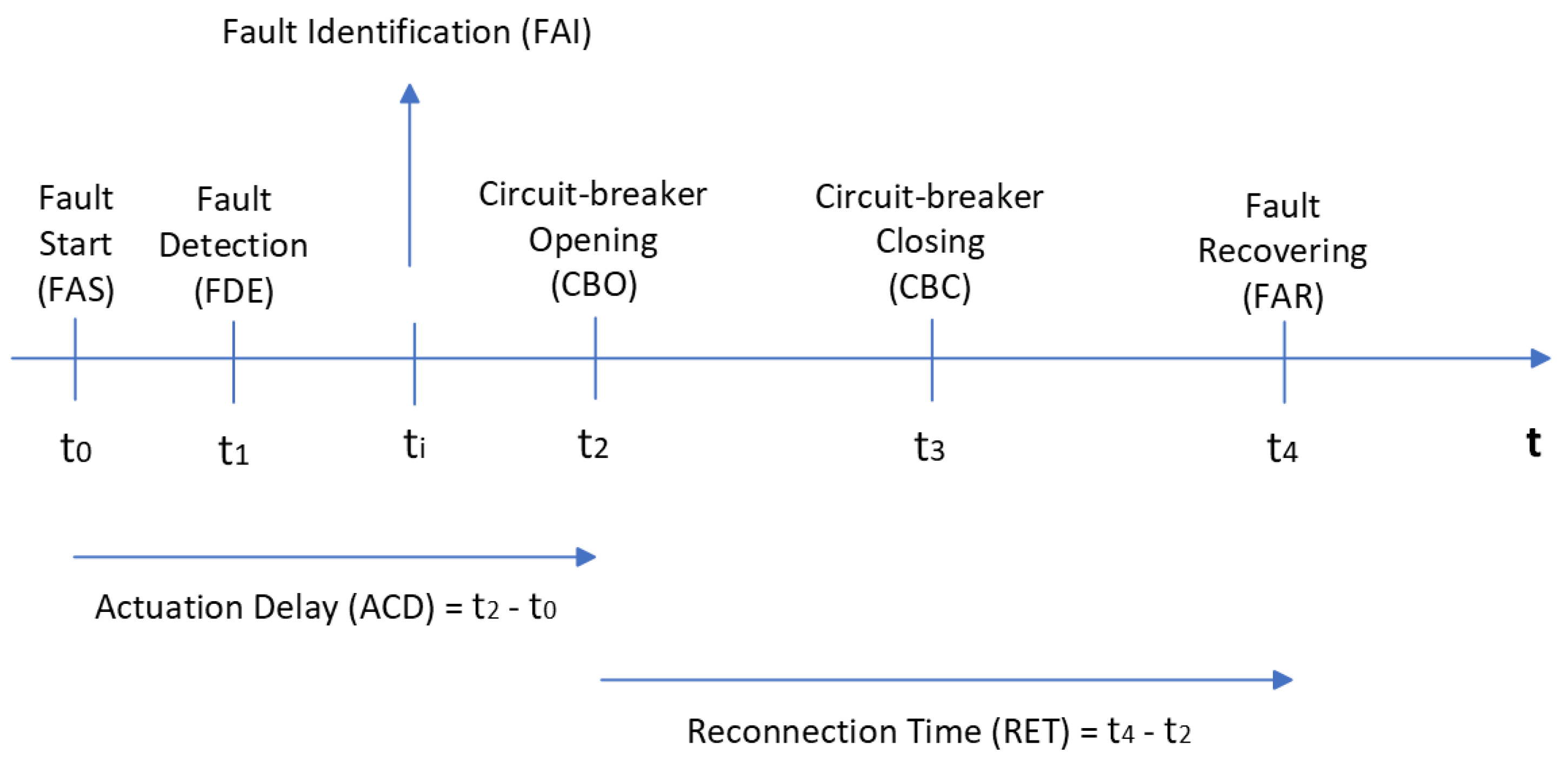
Figure 1. Fault times and circuit breaker actuation times.
Energies 17 02169 g001
Figure 2. High−level architecture of the proposed fault detection and diagnosis (FDD) approach.
Energies 17 02169 g002
Figure 3. Architecture of the fault detection approach.
Energies 17 02169 g003
Figure 4. Nominal voltage data and 2D PCA model (ta1,ta2).
Energies 17 02169 g004
Figure 5. Architecture of the fault diagnosis approach.
Energies 17 02169 g005
Figure 6. Architecture of the fault identification approach.
Energies 17 02169 g006
Figure 7. Fault identification window, with multiple faults (F1 and F5).
Energies 17 02169 g007
Figure 8. Noise and noisy signals in the nominal operating region.
Energies 17 02169 g008
Figure 9. Fault F6 (ABG): current signals (i1, i2, i3, i0).
Energies 17 02169 g009
Figure 10. Fault F6 (ABG): voltage signals (u1, u2, u3, u0).
Energies 17 02169 g010
Figure 11. Fault F6 (ABG)—PCA 2D scores: nominal behavior (left image), behavior with a fault (right image).
Energies 17 02169 g011
Figure 12. Fault F1 (CG)—PCA 2D scores: nominal behavior (left image), behavior with a fault (right image).
Energies 17 02169 g012
Figure 13. Fault F6 (ABG): Fault detection signal, Re , and adaptive threshold.
Energies 17 02169 g013
Figure 14. Fault F6 (ABG): Fault detection and diagnosis.
Energies 17 02169 g014
Figure 15. Fault F6 (ABG): Estimation of the amplitude of i 1 using the SW-DFT.
Energies 17 02169 g015
Figure 16. Fault F6 (ABG): Estimation of the instantaneous frequency of i 1 using the Hilbert transform.
Energies 17 02169 g016
Figure 17. Fault F1 (CG): Fault detection and diagnosis.
Energies 17 02169 g017
Table 1. Notation.
Table 1. Notation.
SymbolMeaning
tContinuous time
kDiscrete time
u Voltage signals
u 1 , u 2 , u 3 Voltage signals in phases A, B, C
u 0 Voltage signal in grounded (earthed) neutral wire
i Current signals
i 1 , i 2 , i 3 Current signals in phases A, B, C
i 0 Current signal in grounded (earthed) neutral wire
A s Amplitude of a signal
TPeriod of a signal
fFrequency of a signal
wAngular frequency of a signal: w = 2 π / T = 2 π f
ϕ Phase of a signal
H x Threshold for the signal x ( k )
t m a x Simulation time in HyperSim: 1.5 s
T s Sampling time in HyperSim: 50 µs
N f Number of CSV files processed for each experiment: 619
nNumber of samples in each signal per experiment in HyperSim: 30,001
aNumber of relevant principal components in the PCA model: a = 2
&&Logical AND
||Logical OR
max()Maximum function
min()Minimum function
Table 2. Relevant references in the FDD area applied to power lines.
ApproachDiagnostics TechniqueReferenceYear
PCA, DFT, and DHTRule-basedThis article2024
Data-based RVFLNs neural methodML/AI[30]2023
Machine learning and variational autoencodersML/AI[47]2023
Wavelets and fuzzy decision systemRule-based[42]2022
PELT and wavelet transformML/AI[44]2022
Machine learning with neural networksML/AI[45]2022
Wavelet transform and neural networksML/AI[46]2022
Deep reinforcement learningML/AI[50]2022
Power quality eventsML/AI[36]2020
Deep graph convolutional networksML/AI[49]2020
Group sparse representationRule-based[37]2019
Wavelets, local energy, and SVMML/AI[48]2017
Table 3. Established SNR values, and neutral current i 0 in nominal operating region.
SNR u [dB] SNR i [dB]| i 0 | [A]
8580<1
5550<1
3530<1
3025<1
2520<1
Table 4. Short-circuit faults and main symptoms.
FaultIDType i 0 i 1 i 2 i 3 u 1 u 2 u 3
F73PThree-Phase to Ground+1+1+1+1−1−1−1
F6ABGTwo-Phase to Ground+1+1+10−1−10
F5ACGTwo-Phase to Ground+1+10+1−10−1
F4AGPhase–Ground+1+100−100
F3BCGTwo-Phase to Ground+10+1+10−1−1
F2BGPhase–Ground+10+100−10
F1CGPhase–Ground+100+100−1
F0F0No Fault0000000
Table 5. PCA model: explained variance as a function of the number of principal components a.
a E σ 2 ( a ) [ % ] Choice
151.3249%
299.9989% a = 2
399.9999%
4100%
Table 6. Short-circuit faults F5, F1, and F0, and main symptoms.
FaultIDType i 0 i 1 i 2 i 3 u 1 u 2 u 3
F5ACGTwo-Phase to Ground+1+10+1−10−1
F1CGPhase–Ground+100+100−1
F0F0No Fault0000000
Table 7. Example of applying the fault identification approach for data depicted in Figure 7.
Case M a M b Fault
C1F1F1F1
C2F0F1F1
C3F1F5F1
C4F1F1F1
Table 8. Thresholds computed in nominal operating region, and SNR dependence.
TaskThresholdsExpressionValueSNR Dependence
Fault Detection H R e ( k ) G d × m a x ( R e ( k N + 1 : k ) ) G d = 1.2Equation (21)
Fault Identification H i x ( k ) G i × m a x ( i x ( k N + 1 : k ) ) G i = 1.2Equation (24)
Fault Identification H u x ( k ) G u × m a x ( u x ( k N + 1 : k ) ) G u = 0.95Equation (25)
Circuit Breaker Opening H i x 2 1.0 A
Circuit Breaker Closing H i x 2 1.0 A
Fault Recovery d f 15 Hz
Table 9. HyperSim simulator parameters.
ParameterMinimum ValueMaximum ValueVariation
Start of fault0.1 s0.3 s0.01 s
Circuit breaker openingStart of fault + 0.04 sStart of fault + 0.06 s0.001 s
End of faultCircuit breaker closing − 0.06 sCircuit breaker closing − 0.04 s0.001 s
Circuit breaker closingCircuit breaker opening + 0.9 sCircuit breaker opening + 0.9 s0 s
Fault location40% of the line length60% of the line length10% of the line length
Fault resistance (ohm)2201
Table 10. Short-circuit faults and some file examples.
FaultIDTypeFile
F73PThree-Phase to Ground“LCGRM1_4_15_30_43.csv”
F6ABGTwo-Phase to Ground“LCGRM1_1_11_15_54.csv”
F5ACGTwo-Phase to Ground“LCGRM1_2_12_36_39.csv”
F4AGPhase–Ground“LCGRM1_5_17_16_58.csv”
F3BCGTwo-Phase to Ground“LCGRM1_3_14_18_05.csv”
F2BGPhase–Ground“LCGRM1_6_18_21_34.csv”
F1CGPhase–Ground“LCGRM1_7_20_24_10.csv”
F0F0No Fault
Table 11. Main simulation parameters and times.
Parameters/TimesValue
HyperSim simulation parametersSee Table 9
Simulation time in HyperSim, t m a x 1.5 s
Sampling time in HyperSim, T s 50 µs
Number of samples in each signal generated by HyperSim, n 30 , 001
Number of CSV files processed in Python619
CPU processing time for each CSV file 58.22 s
Number of Portuguese overhead power lines simulated12
Voltages on power lines [kV] 150 , 220 , 400
SNR i [dB] in current signals20, 25, 30, 50, 80
SNR u [dB] in voltage signals25, 30, 35, 55, 85
Load variations on power linesYes
Low-, medium-, and high-impedance short-circuit faultsYes
Fault start estimation, t 0 | i 0 | > 1 A
Fault detection parameters G d = 1.2
Fault identification parameters G i = 1.2, G u = 0.95
Fault identification window size60 or 80 ms
Table 12. FDD main simulation results without noise (SNR = + ).
FaultIDSimFDDFDD-Sim
F73P90900
F6ABG8782−5
F5ACG8983−6
F4AG9091+1
F3BCG86860
F2BG8790+3
F1CG9095+5
Fxxyz02+2
Σ 6196190
Table 13. FDD main simulation results for different SNR i .
FaultIDSim20 dB25 dB30 dB50 dB80 dB
F73P909090909090
F6ABG878483828282
F5ACG898687858483
F4AG908789929191
F3BCG868484848686
F2BG878991919090
F1CG909794959695
Fxxyz021002
Σ 619619619619619619
Table 14. Main global performance (accuracy) indices, η [ % ] , for different SNR i .
TaskID20 dB25 dB30 dB50 dB80 dB
Fault Detection [%]FDE100100100100100
Fault Identification [%]FDI97.0997.9098.2298.0697.58
Table 15. Average values of times and delays for different SNR i .
Times and Delays [ms]20 dB25 dB30 dB50 dB80 dB
Fault Detection Delay: t 1 t 0 4.831.640.910.800.81
Fault Identification Delay: t i t 1 60.1960.1960.2660.7761.00
CB Actuation Delay: t 2 t 0 58.9459.1059.2259.4159.81
CB Reconnection Time: t 4 t 2 929.62929.62929.62929.62929.62
Table 16. Performance comparison with other studies in the literature.
ApproachReferenceDataset/SWNoiseAccuracy [%]
Rule-Based: PCA, DFT and DHTThis ArticleREN: HyperSimYes98.22
Deep reinforcement learning[50]IEEE 14-busYes100.00
Wavelets, local energy and SVM[48]PSCADYes99.77
Deep graph convolutional networks[49]IEEE 123-busYes99.38
Group sparse representation[37]PSCADYes99.09
Machine learning and variational autoencoders[47]AspenNo99.00
Wavelet transform and neural networks[46]REN: HyperSimNo98.50
Machine learning with neural networks[45]Matlab/SimulinkYes98.47
Wavelets and fuzzy decision system[42]IEEE 34-busNo94.90
Power quality events[36]Real Smart GridNo92.90
PELT and wavelet transform[44]REN: Real DataNo91.56
Data-based RVFLNs neural method[30]RTDS-RTSYes89.94
Disclaimer/Publisher’s Note: The statements, opinions and data contained in all publications are solely those of the individual author(s) and contributor(s) and not of MDPI and/or the editor(s). MDPI and/or the editor(s) disclaim responsibility for any injury to people or property resulting from any ideas, methods, instructions or products referred to in the content.