The Efficiency of the Kalman Filter in Nodal Redundancy

Abstract

The growing integration of distributed energy resources underscores the critical importance of having precise insights into the dynamics of an electrical power system (EPS). Consequently, an estimator must align with the EPS dynamics to enhance the overall reliability, safety, and system stability. This alignment ensures that operators can make informed decisions during system operations. An initial step in gaining insight into the system’s state involves examining its state vector, which is represented by voltage phasors. These results are derived through the application of a distributed state-estimation process in large-scale systems. This study delved into the effectiveness of Bayesian filters, with a particular emphasis on the extended Kalman filter (EKF) algorithm in the context of distributed state estimation. To analyze the outcomes, the nodal partitioning process was incorporated within the distributed state-estimation framework. The synergy between the EKF algorithm and the partitioning method was evaluated using the IEEE118 test system.

1. Introduction

The significance of having information to ascertain the state of an electrical power system (EPS) cannot be overstated. It enables system operators (SOs) to make prompt decisions that prevent operational disruptions and potential blackouts within the electrical network [1,2]. A pivotal tool in achieving this objective is a state estimator. This technology ensures that power demands are met while adhering to operational constraints, including transmission line capacities, voltage limits, and generation limits [3,4,5].

In the process of monitoring a system, the role of a state estimator (SE) is to determine or approximate the optimal value of a deterministic or random variable. These variables are often challenging to directly capture through measurement systems [6]. Consequently, state estimators hold a pivotal position in the energy industry due to their essential role in establishing the state of an electrical system [7]. Estimators play a crucial role by providing essential information about a system’s state, allowing for the real-time assessment of voltage phasors at different locations within the system. This task involves handling extensive data volumes at a control center, which, in turn, leads to increased costs related to economic and computational resources [8]. Within the estimation process, it becomes essential to analyze measurement redundancy to mitigate the risk of deviations or errors in the applied algorithm.

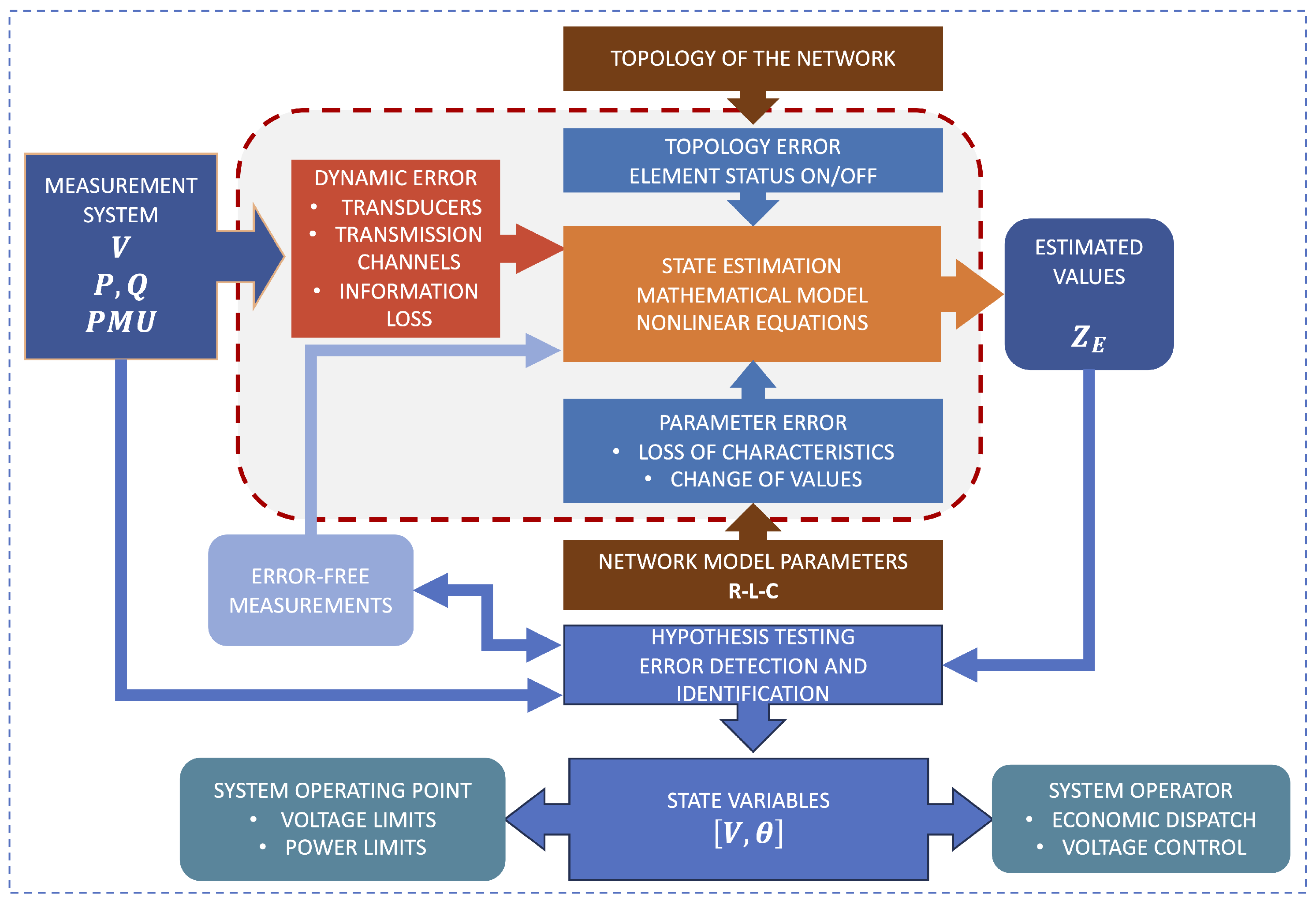
The architecture of state estimators has evolved with the development of new algorithms, Figure 1. In the centralized estimation model, a single control center is required to process all the measurements of an EPS; however, today, distributed processes are applied, making it necessary to partition a system and reduce the problem to subproblems, where the estimator is applied in this new configuration. Several methods for partitioning have been proposed in the literature [9,10].

Estimators play a pivotal role in providing crucial insights into the system’s status. They enable the real-time assessment of voltage phasors at various points within the system. However, this task involves the management of substantial data volumes at a central control center, leading to increased costs related to economic and computational resources [8]. Within the estimation process, it is essential to scrutinize measurement redundancy to mitigate the risk of deviations or errors in the applied algorithm. In contemporary times, the architecture of state estimators has evolved with the development of new algorithms. While the conventional centralized estimation model required a single control center to process all the measurements of an EPS, modern practices favor distributed processes. Consequently, system partitioning is necessary, allowing the problem to be divided into subproblems where the estimator is applied. Various partitioning methods have been proposed in the literature to address this evolving landscape.

The Kalman filter and its extension, namely, the extended Kalman filter (EKF), represent fundamental tools in the precise and up-to-date estimation of the state of dynamic systems, playing a crucial role in a wide range of fields from electrical engineering to robotics [11,12]. These algorithms are especially relevant in environments where the fusion of information from multiple sources is imperative to obtain reliable estimates of the system state. Furthermore, the Kalman filter, along with its extended variant, is capable of effectively handling the noise present in both measurements and the system model, making them valuable tools for situations where measurements may be subject to significant disturbances.

On the other hand, the weighted least squares (WLS) method offers an alternative strategy for system state estimation, focusing on minimizing the mean squared error between measurements and state estimates. This method is particularly useful when available measurements exhibit varying levels of uncertainty, as it allows for assigning different weights to each measurement based on its perceived reliability. In situations where precision and reliability are critical, the weighted least squares approach can provide more accurate estimates of the system state by prioritizing the most reliable measurements.

In summary, both the Kalman filter and its extension, as well as the weighted least squares method, are powerful tools in system state estimation, each with its own advantages and specific applications. Their effective use enables obtaining precise and up-to-date estimates of the system state in a variety of applications, from monitoring electrical systems to autonomous vehicle navigation.

It is important to note that [13] both the EKF and WLS have their respective advantages and limitations. The EKF excels when dealing with noisy measurements and when highly accurate state estimation of the system is required, although its implementation requires a dynamic model of the system and can result in a significant computational burden. On the other hand, WLS is suitable for situations where measurements come with different levels of precision, although its ability to maintain accuracy in the presence of high noise levels may be more limited compared with the EKF [14].

The main differences between WLS and the EKF can be summarized as follows:

• Application domain: WLS—Primarily used for curve fitting and regression tasks, where the objective is to find the parameters of a mathematical model that best fit the observed data. EKF—Mainly applied for state estimation in nonlinear dynamic systems. It is particularly useful when the relationships of the system and measurement equations cannot be linearly modeled.
• Problem type: WLS—Used for curve-fitting and regression problems, with the aim to find coefficients of a mathematical model that describes the relationship between variables. EKF—Designed for state-estimation problems in dynamic systems, such as object tracking or estimating positions and velocities in nonlinear systems.
• Treatment of nonlinearities: WLS—Not specifically designed to handle nonlinearities in the relationships between variables. EKF—Handles nonlinear systems by linearizing the dynamic and measurement equations around the current estimated state.
• Mathematical approach: WLS—Relies on the least squares method, minimizing the sum of squared weighted errors between observed and model-predicted data. EKF—Utilizes the theory of Kalman filters and linear approximation to perform estimation in nonlinear systems.

In essence, WLS is focused on fitting models to observed data, while the EKF is geared toward estimating states in dynamic systems, particularly nonlinear ones. Each method is tailored to address specific challenges and objectives in estimation and modeling [15,16].

The choice between these methods will depend on the specific characteristics of the system under consideration and the properties of the available measurements. This choice is crucial to ensure an effective state estimation of the system.

A dynamic state estimation is a technique, as described in [17], that tracks changes in the state variables within a power system. However, there is no precise physical modeling of the system’s time behavior when monitoring changes. Dynamic behavior in estimators is applied when the actual modeling attributed to time variables changes during operation. The advantage of a Bayesian filter provides certain benefits in terms of computational correctness and minimal measurement error in state estimation. To achieve this, it uses information from the state vector over time, as well as the physical model corresponding to the considered system [18,19].

Another concept to consider within the estimation process is network partitioning. Kron and Happ were pioneers in the study of diakoptica, which aims to break down large systems into smaller ones. This underscores the significance of reducing the computational processes associated with analyzing large-scale systems [20].

The DSE anticipates the system’s capability in the time interval $(t+1)$. As a result, DSE algorithms play a significant role in state-estimation techniques [9,21] and have the ability to impact the character of real-time monitoring and control operation. In [22], the importance of demand behavior is highlighted, as it exhibits load variations that increase and decrease over time, causing rapid changes. This dynamic nature of the load makes the model complex, turning the power system into a dynamic system. The monitoring and control of energy systems become highly complex and significant as a result. The role of the state estimator is to provide optimal real-time data on the state vector, relying on a minimum set of measurements. Therefore, the concept of state estimation plays a crucial role in ensuring the safe and economical operation of large-scale interconnected power systems. Depending on the desired states, power system state estimation can be formulated as a static or dynamic process [23].

In the MATLAB 9.14 (R2023a) environment (Mathworks, Inc., Natick, MA, USA), a code was developed to implement the distributed estimator process under the nodal redundancy criterion proposed in [24] and the recursive EKF filter implementation in order to determine the efficiency of the model in the operation of an electrical power system.

The application of the Kalman filter in a state estimator for power systems through nodal partitioning aims to determine whether there is an improvement in the accuracy and reliability of the state vector. The analysis of the results involves assessing the reduction in measurement errors, effective management of uncertainty, optimization of control strategies, and integration of multiple sources of information to achieve a more precise and coherent estimation of the system state.

The article is organized as follows. First, Section 2 describes the integration of the recursive filter within the nodal partitioning method. Second, Section 3 develops the model in the distributed state-estimation process using the EKF for a large-scale system. Next, in Section 4, the simulation results of the analyzed model are presented. The discussion unfolds in Section 5, and finally, the conclusions are summarized in Section 6.

2. Bayesian Recursive Filters

Bayesian filters are a class of algorithms used in statistical estimation theory to infer the state of a system from incomplete or noisy observations. These filters are based on Bayes’ theorem, which allows for updating beliefs about the system’s state as new observations are acquired.

$$p\left(A_i\mid B\right)=\frac{p\left(A_i\cap B\right)}{p\left(B\right)}=\frac{p\left(B\mid A_i\right)p\left(A_i\right)}{{\sum }_{j=1}^{n}p\left(B\mid A_j\right)p\left(A_j\right)}$$

(1)

The Bayesian approach in state estimation aims to construct the posterior probability distribution of a state by considering all available information, including the set of received measurements. This type of estimator is known as a recursive filter [7,10], as it processes received data sequentially rather than in a batch manner, thus avoiding the need to store all the data. The recursive filter consists of two basic stages: the prediction (a priori) stage and the update (a posteriori) stage.

In the prediction stage, the motion model is used to forecast the state of the posterior probability distribution at time $t+1$. It is important to consider that the state is subject to disturbances and is modeled as Gaussian noise. The prediction stage shifts, distorts, and expands the prior probability distribution. In the update stage, the measurement at time $t+1$ is used to modify the prediction of the probability distribution. This stage incorporates measurement information and adjusts the posterior distribution.

Significant developments related to dynamic modeling and the establishment of a state space have been proposed in the literature. From this perspective, it is necessary to establish a model that captures the system and can be mathematically represented. To do this, the plant system must be modeled, and a model that relates observations or measurements must be established. In the context of an electrical power system, nonlinear equations are used to model its dynamics [6]. Below are the equations that define a state space:

$$\begin{array}{cc}\hfill & x_t=f\left(x_{t-1},w_{t-1}\right)\hfill \\ \hfill & z_t=h\left(x_t,v_t\right)\hfill \end{array}$$

(2)

Equation (2) describes the evolution from state $x_{t-1}$ to state $x_t$ over the time interval between $t-1$ and t. This evolution is associated with the error $w_{t-1}$, which represents the uncertainty in state update. These models have a prior probability distribution $p\left(x_t\right|x_{t-1})$, which reflects the available information about the state at time $t-1$ to predict the state at time t.

Equation (3) presents the observation model, which relates the measurement $z_t$ to the current value of the state $x_t$. In this equation, the term $v_t$ is associated with the stochastic measurement error and reflects its uncertainty. A probability distribution of the measurement $p\left(z_t\right|x_t)$ can be inferred from this equation, which describes the probability of obtaining the measurement $z_t$ given the state $x_t$.

A state space is developed through a model that represents the evolution of the state vector based on the imposed control signals. In Blood et al. [25,26], a plant model is proposed based on the nodo balance equation:

$$f_i(x,\Gamma )=V_i{e}^{j{\delta }_i}\sum V_k{Y}_{ik}{e}^{j\left({\delta }_j+{\varphi }_{ik}\right)}-\left(P_i+j{Q}_i\right)=0$$

(3)

where $\Gamma ={\left[\begin{array}{c}{P}_1{P}_2\dots P_N{Q}_1{Q}_2\dots \dots Q_N\hfill \end{array}\right]}^T$ represents the vector of the active and reactive power injections of dimension 2N.

Differentiating $f_i(x,\Gamma )$ with respect to x and $\Gamma$, we have

$$\frac{\delta f_i(x,\Gamma )}{\delta x}dx+\frac{\delta f_i(x,\Gamma )}{\delta \Gamma }d\Gamma =0$$

(4)

$$\mathbf{H}=\frac{\delta f_i(\mathbf{x},\Gamma )}{\delta \mathbf{x}}$$

(5)

$$\mathbf{I}=\frac{\delta f_i(x,\Gamma )}{\delta \Gamma }$$

(6)

$$Hdx+Id\Gamma =0$$

(7)

where H turns out to be the Jacobian matrix of the state vector, while I represents the identity matrix. Solving for $dx$ from (7), we have

$$dx=-{\mathbf{H}}^{-1}d\Gamma$$

(8)

The differential $dx$ represents the infinitesimal variation between two static operating points $(x_1,{\Gamma }_1)$ and $(x_2,{\Gamma }_2)$, which satisfies Equation (7). Linearizing the differential as an incremental relationship and considering a process error $w_l$, Equation (8) can be expressed as follows:

$$\Delta x=\left(x_1-x_2\right)=-{\mathbf{H}}^{-1}\left({\Gamma }_1-{\Gamma }_2\right)+w_l$$

(9)

By considering that the two operating points are static within a time interval from t to $t+Ts$, it allows the model to be represented as:

$$x\left[t+T_s\right]=x\left[t\right]-{\mathbf{H}}^{-1}u\left[t\right]+w_l$$

(10)

where the vector $u\left[t\right]=\Delta \Gamma \left[t\right]=\Gamma \left[t+T_s\right]-\Gamma \left[t\right]$ represents the change in system operation over time due to demand dependency. Equation (10) presents the model that associates both the new operating point and the previous one with a power variation $u\left[t\right]$ when the system changes its operating point due to the dynamic behavior of the demand.

2.1. Extended Kalman Filter (EKF)

The EKF, being a recursive algorithm, estimates the state of a system that evolves over time due to the demand behavior of an electrical power system. This filter is considered optimal, as it minimizes a specific criterion using all available information from the previous state for filtering. The term recursive means that it does not require the storage of previous data, thus facilitating its implementation in real-time processing systems.

The main goal of the EKF is to optimally estimate states, minimizing the mean squared error index. Unlike WLS, the EKF leverages the system state information to improve the estimation accuracy. This is achieved by using a dynamic model that describes the state’s evolution over time and the propagation of associated uncertainty. As new measurements are received, the EKF updates the state estimation using both the dynamic model and available measurements. In the literature, various studies highlighted the advantages of the EKF compared with other methods, such as WLS. These studies emphasized the use of system state information as a key factor in improving the estimation accuracy [6,27].

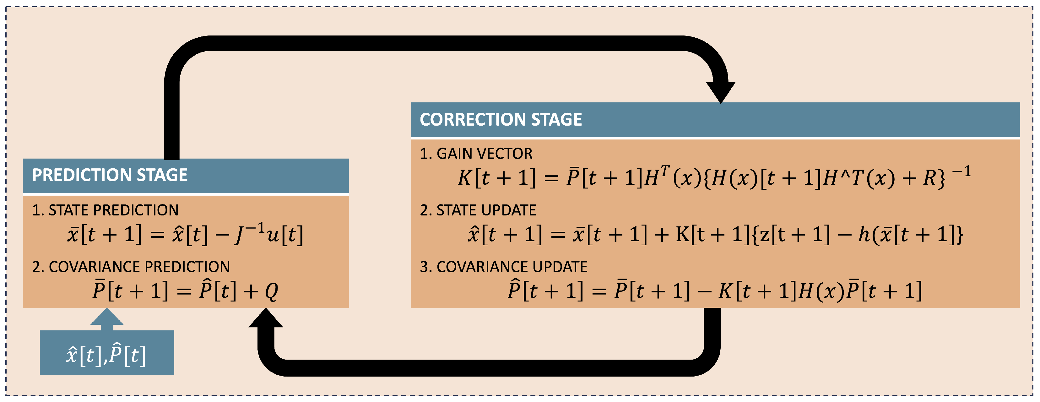
All these criteria and concepts provide us with the guidelines for implementing the extended Kalman filter algorithm by considering two stages in the voltage phasor $[\mathbf{V},\theta ]$ estimation process:

• In the prediction stage at $t+1$, the prediction of the state vector and the measurement covariance matrix are evaluated.

  $$\overline{\mathbf{x}}\left[t+T_s\right]=\widehat{\mathbf{x}}\left[t\right]-{\mathbf{H}}^{-1}\mathbf{u}\left[t\right]$$

  (11)

  $$\overline{\mathbf{P}}\left[t+T_s\right]=\widehat{\mathbf{P}}\left[t\right]+\mathbf{Q}$$

  (12)
• In the correction stage of the estimation, given the dynamic behavior of demand that generates a new operating point over a timeline, the measurement at instant $t+1$ is taken, allowing for the calculation of the gain matrix. This updates the estimation of the state vector and the covariance.

  $$\mathbf{K}\left[t+T_s\right]=\overline{\mathbf{P}}\left[t+T_s\right]{\mathbf{H}}^T\left(x\right){\left\{\mathbf{H}\left(x\right)\overline{\mathbf{P}}\left[t+T_s\right]{\mathbf{H}}^T\left(x\right)+\mathbf{R}\right\}}^{-1}$$

  (13)

  $$\widehat{\mathbf{x}}\left[t+T_s\right]=\overline{\mathbf{x}}\left[t+T_s\right]+\mathbf{K}\left[t+T_s\right]\left\{\mathbf{z}\left[t+T_s\right]-\mathbf{h}\left(\overline{\mathbf{x}}\left[t+T_s\right]\right)\right\}$$

  (14)

  $$\widehat{\mathbf{P}}\left[t+T_s\right]=\overline{\mathbf{P}}\left[t+T_s\right]-\mathbf{K}\left[t+T_s\right]\mathbf{H}\left(x\right)\overline{\mathbf{P}}\left[t+T_s\right]$$

  (15)

  where
  $\mathbf{K}$—Kalman gain;
  $\widehat{\mathbf{x}}$—estimation at $t+T_s$ (update);
  $\mathbf{H}$—Jacobian matrix construction;
  $\mathbf{R}$—inverse matrix of the measurement covariance matrix w;
  $\mathbf{x}$—system measurements or observations.

This process allows for estimating the state vector by considering an a priori system state. Figure 2 illustrates the extended Kalman filter algorithm.

The EKF approximates the nonlinear functions of the model using a first-order Taylor series expansion to optimal terms, assuming that this approximation is sufficient to describe the system’s dynamics. However, this approximation can decrease the filter’s performance and even convergence because a fundamental feature of the EKF is that it always approximates $p(x_t/z_t)$ to a Gaussian distribution, which can be a drawback if its probability density function (pdf) is not Gaussian. Additionally, another problem is that it requires the construction of Jacobian matrices, which is not trivial and can lead to difficult-to-detect errors. It is important to mention that the equations modeling the state space must be differentiable; otherwise, this filter cannot be applied. In this context, the literature presents certain improvements, such as the unscented Kalman filter (UKF).

2.2. Nodal Grouping

Traditionally, power grid state estimation has relied on a centralized architecture. However, with the deregulation of grids and growing concerns about information privacy and security, there has been a shift toward multi-area state estimation. Current state-of-the-art solutions often employ a weighted norm of a residual measurement model, which may obscure gross errors concealed within the null space of the Jacobian matrix. To address this issue, we propose a distributed innovation-based model. This approach utilizes measurement innovation to effectively tackle error composition [28].

Clustering is a technique used to group items that share similar characteristics. Various clustering methods have been developed, including K-means, electrical distance, spectral clustering, and hierarchical clustering algorithms [24,29,30]. The proposed nodal grouping method is based on the set of measurements associated with the buses of an electrical system. The objective of this estimation model is to create areas or regions within the system where measurements are distributed in such a way that the redundancy within these regions is as uniform as possible.

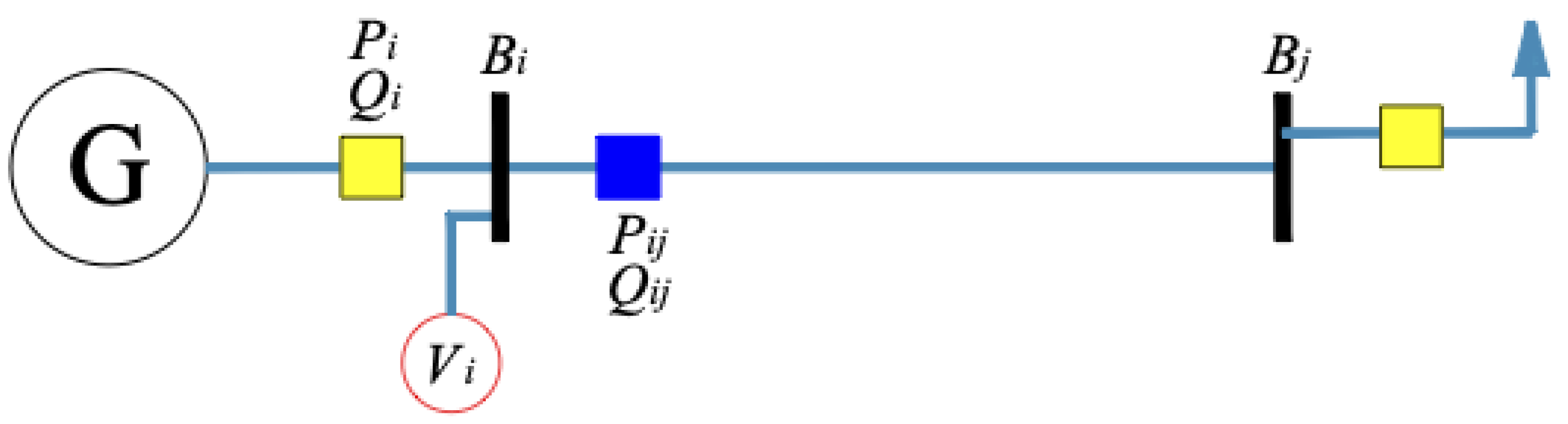
The nodal grouping principle involves determining which measurements belong to a specific bus. To achieve this, two types of measurements are established: bus measurements ($M_B$) and line measurements ($M_l$). Figure 3 illustrates the physical arrangement of measurements in an electrical system.

In the realm of $M_B$ measurements, those directly linked to the system bus can be categorized into two distinct types: voltage measurements $M_V$ on the one hand, and active power $M_P$ and reactive power $M_Q$ injection measurements on the other. These measurements are typically associated with connections between generators and buses or loads and buses. Therefore, for the i-th bus, we encounter the following:

$$M_{Bi}=\left\{\begin{array}{c}{M}_{Vi}\hfill \\ M_{Pi}\hfill \\ M_{Qi}\hfill \end{array}\right.$$

(16)

The measurement data defined as $M_l$ are the active and reactive power flow measurements between node i and node j, and the membership of the measurement will be established with the closest bus under the following consideration:

$${\mathit{M}}_l=\left\{\begin{array}{ccc}{\mathit{M}}_{Pij}\hfill & \in \hfill & {\mathbf{B}}_i\hfill \\ {\mathit{M}}_{Qij}\hfill & \in \hfill & {\mathit{B}}_i\hfill \end{array}\right.$$

(17)

Consequently, the set of all measurements affiliated with bus i is outlined as follows:

$$M_i=M_{Bi}+M_{Li}$$

(18)

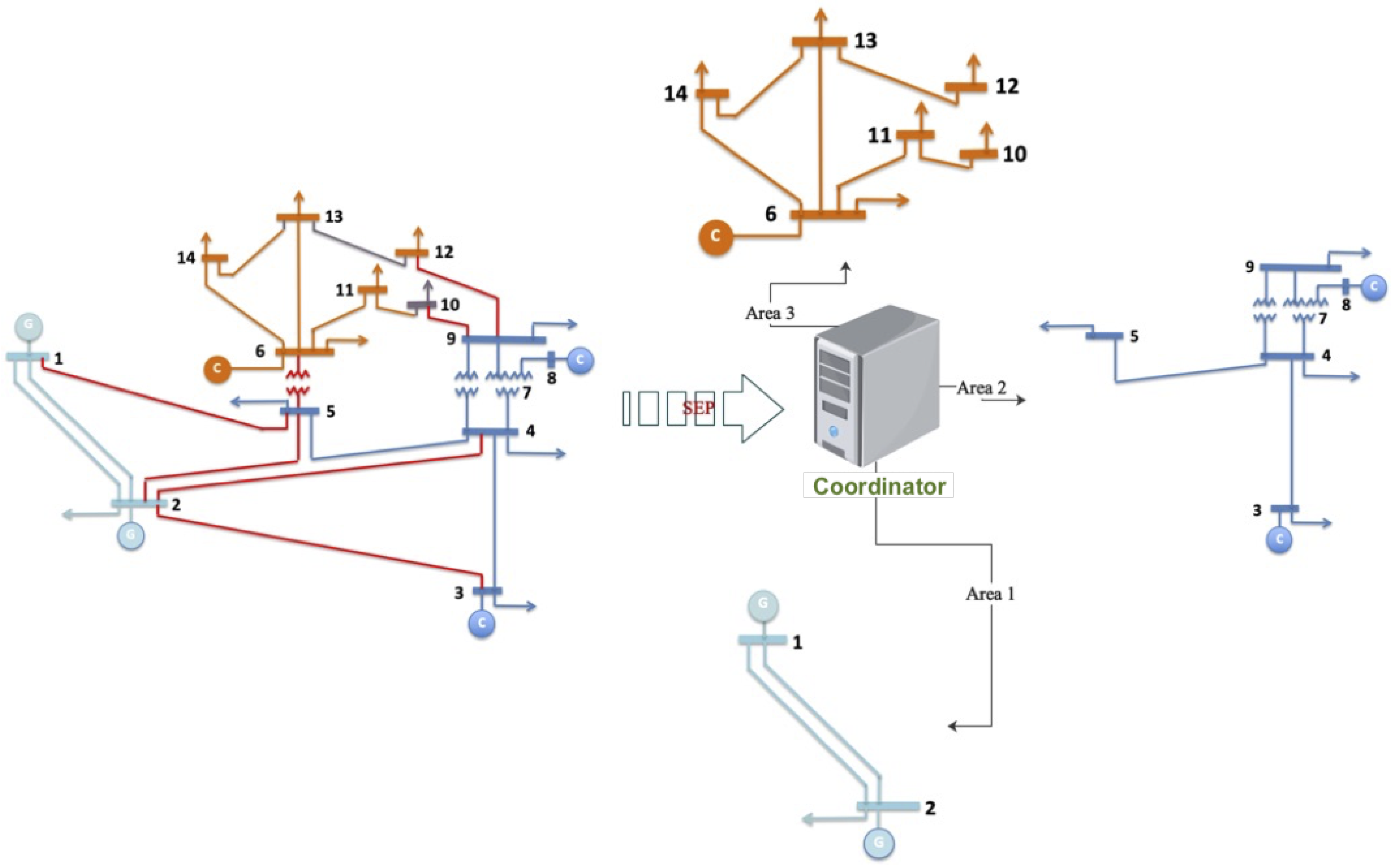
2.3. Nodal Partition Method

When implementing a distributed state estimator (DSE), the initial system is divided into multiple groups or subsystems. At this stage, a local estimate is computed using measurements from each cluster. Subsequently, the overall estimate of the electrical system is determined by integrating the information from neighboring measurements across the subsystems; see Figure 4.

2.4. Preliminary Concept

1.

State estimation: The state-estimation process for an AC system relies on a mathematical model comprising nonlinear functions. These functions establish a relationship between the set of measurements and the system’s state variables:

$$\mathbf{z}\mathbf{=}\mathbf{h}\mathbf{\left(}\mathbf{x}\mathbf{\right)}\mathbf{+}\mathbf{e}$$

(19)

where

$\mathbf{x}$: state vector 2N, [V,$\theta$];

$\mathbf{z}$: set of measurements M ($M>2$N concept of observability);

$\mathbf{h}$: set of nonlinear functions;

$\mathbf{e}$: error present in the measurements.

In traditional state-estimation models, the state vector is defined by the voltage phasor $[V,{\theta }_0]$, and the measurement set includes voltage magnitudes ${\mathit{V}}_{\mathit{i}}^h$, active and reactive power injections, and active and reactive power flows [17]. The nonlinear equations that establish the relationship between the state variables in the electric power system model are

$$\begin{array}{c}{P_i}^m={\displaystyle \sum _{j=1}^N}{V}_i{V}_j\left(G_{ij}cos{\theta }_{ij}+B_{ij}sin{\theta }_{ij}\right)\\ {Q_i}^m={\displaystyle \sum _{j=1}^N}{V}_i{V}_j\left(G_{ij}sin{\theta }_{ij}-B_{ij}cos{\theta }_{ij}\right)\\ {P_{ij}}^n=V_i{V}_j\left(G_{ij}cos{\theta }_{ij}+B_{ij}sin{\theta }_{ij}\right)-G_{ij}{V}_i^2\\ {Q_{ij}}^n=V_i{V}_j\left(G_{ij}sin{\theta }_{ij}-cos{\theta }_{ij}\right)-V_i^2\left(B_{ij}-b_{ij}\right)\end{array}$$

(20)

In the estimator model, the objective function is minimized to assess the error between the estimated measurements and the actual measured values [7].

$$minJ=\sum _1^M\frac{{\left(z_i-h_i\left(\widehat{\mathit{x}}\right)\right)}^2}{{\sigma }_i^2}={\left[\mathbf{z}-{\mathit{H}}_x\right]}^T\mathbf{W}\left[\mathbf{z}-{\mathit{H}}_x\right]$$

(21)

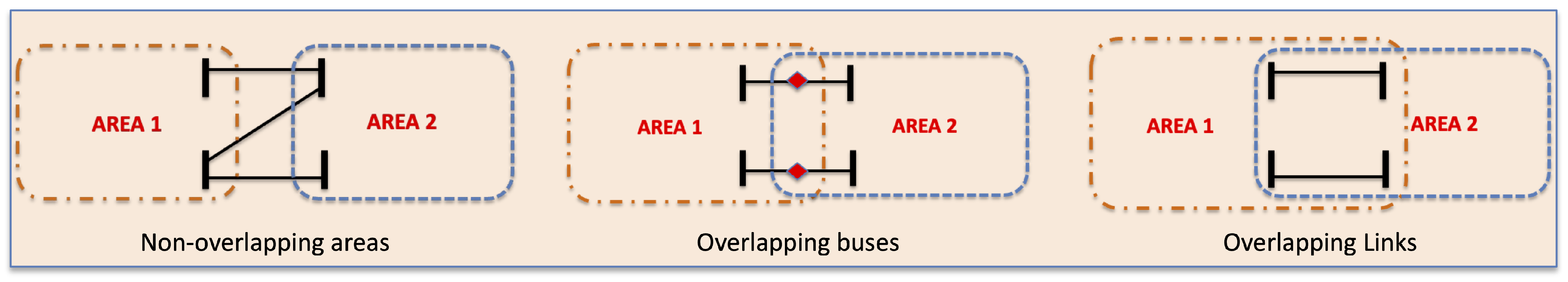
2.

Grouping concept: During the system partitioning process, interconnected areas may exhibit varying physical configurations (Figure 5):

• Non-overlapping areas consist of buses that belong exclusively to one area. The connection between these areas is established through their transmission systems.
• In overlapping buses, the buses are part of multiple areas within the partition.
• In overlapping links, the configuration accounts for the fact that the link between two buses belongs to multiple overlapping areas.

Figure 5. Physical arrangement.

Figure 5. Physical arrangement.

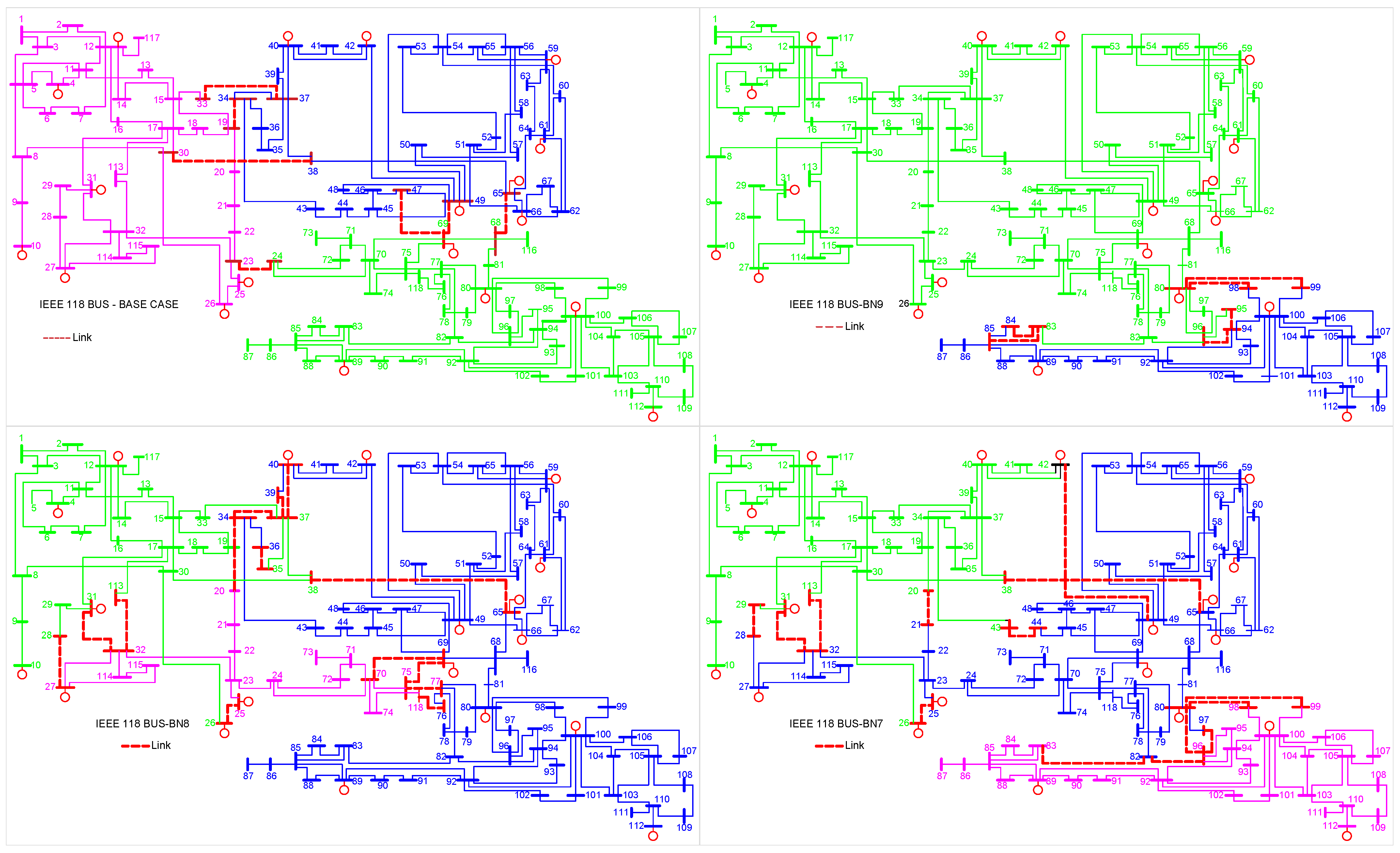
According to [24], the EPS is divided into non-overlapping areas, ensuring the physical connection of subsystems through the transmission system. The observability criterion must be met for the entire system and for each area into which it is divided. If an area is not observable, pseudo-measurements are used to restore observability.

3.

Nodal buses: these buses concentrate the largest number of measurements:

$$B{N}_k=max(\#M)$$

(22)

4.

Node links: After determining the nodal buses (BNs), the areas are constructed, where the neighboring buses connected through the transmission system must be linked. In each iteration, the subsystems grow radially. The system expands through the lines connecting the nodes, and the number of buses increases with each iteration.

5.

Overlapping criteria: In the proposed methodology, expanding areas may cause overlapping, where a bus can be part of multiple areas due to system connections. To resolve this, the redundancy error minimization criterion is used to assign overlapping buses to one area, ensuring homogeneity in redundancy values. Figure 6 shows how systems are divided under the concept of nodal redundancy.

3. Problem Formulation

Integrating the extended Kalman filter (EKF) into a distributed state estimation (DSE) requires dividing the power system into several groups (subsystems). In each of these groups, a local estimation is performed using the EKF algorithm based on the measurements from that specific group. Following this stage, the entire system is integrated with information from neighboring subsystems to determine the global estimation. The distributed estimation process involves applying the EKF algorithm in each subsystem for local estimation (Figure 4). Subsequently, a global system is constructed that performs a correction based on the information from its boundaries, which allows for a global estimation of the system.

Power system dynamics can be represented as a set of nonlinear equations, such as

$$\begin{array}{cc}\hfill & {\underline{x}}_{t+1}=f\left({\underline{x}}_t,{\underline{\omega }}_t\right)\hfill \\ \hfill & {\underline{z}}_t=h\left({\underline{x}}_t,{\underline{\delta }}_t\right),\hfill \end{array}$$

(23)

In this context, ${\underline{x}}_t$ represents the state vector, ${\underline{z}}_t$ corresponds to the measurement vector, ${\underline{\omega }}_t$ is the white Gaussian noise vector, ${\underline{\delta }}_t$ stands for the measurement noise vector at time instance t, and $f(.)$ and $h(.)$ are nonlinear functions in vector form that describe the system and state equations. The dimensions of these vectors are all $1\times N$, where N represents the number of buses in the system. The state of each bus at time t, denoted as $x_{i,t}$, can be defined by its attributes, such as $v_{i,t}$ or ${\theta }_{i,t}$. Here, $v_{i,t}$ and ${\theta }_{i,t}$ represent the voltage and phase angle at bus i during time t, respectively. Additionally, the measurements at bus i during time t, represented as $z_{i,t}$, can encompass attributes like ${\mathbf{p}}_{i,t}$, ${\mathbf{q}}_{i,t}$, $v_{i,t}$, and ${\theta }_{i,t}$. In this context, ${\mathbf{p}}_{i,t}$ and ${\mathbf{q}}_{i,t}$ refer to real and reactive power injections, respectively. The objective of the state-estimation process here is to estimate the vector ${\underline{x}}_{t+1}$ based on the measurement vector ${\underline{z}}_t$. As explained in [6], traditionally, state estimation has been addressed using dynamic complex power flow equations, such as

$$\begin{array}{cc}\hfill & {\mathbf{p}}_{i,t}=\sum _{j=1}^N\left|v_{i,t}\right|\left|v_{j,t}\right|\left|Y_{ij}\right|cos\left({\theta }_{i,t}-{\theta }_{j,t}-{\Delta }_{ij}\right)\hfill \\ \hfill & {\mathbf{q}}_{i,t}=\sum _{j=1}^N\left|v_{i,t}\right|\left|v_{j,t}\right|\left|Y_{ij}\right|sin\left({\theta }_{i,t}-{\theta }_{j,t}-{\Delta }_{ij}\right)\hfill \\ \hfill & {\mathbf{p}}_{ij,t}=\left|v_{i,t}\right|\left|v_{j,t}\right|\left|Y_{ij}\right|cos\left({\theta }_{i,t}-{\theta }_{j,t}-{\Delta }_{ij}\right)-G_{i}j{\left|v_{i,t}\right|}^2\hfill \\ \hfill & {\mathbf{q}}_{ij,t}=\left|v_{i,t}\right|\left|v_{j,t}\right|\left|Y_{ij}\right|sin\left({\theta }_{i,t}-{\theta }_{j,t}-{\Delta }_{ij}\right)-(B_{i}j-b_{i}j){\left|v_{i,t}\right|}^2\hfill \end{array}$$

(24)

4. Simulation and Results of Application of EKF

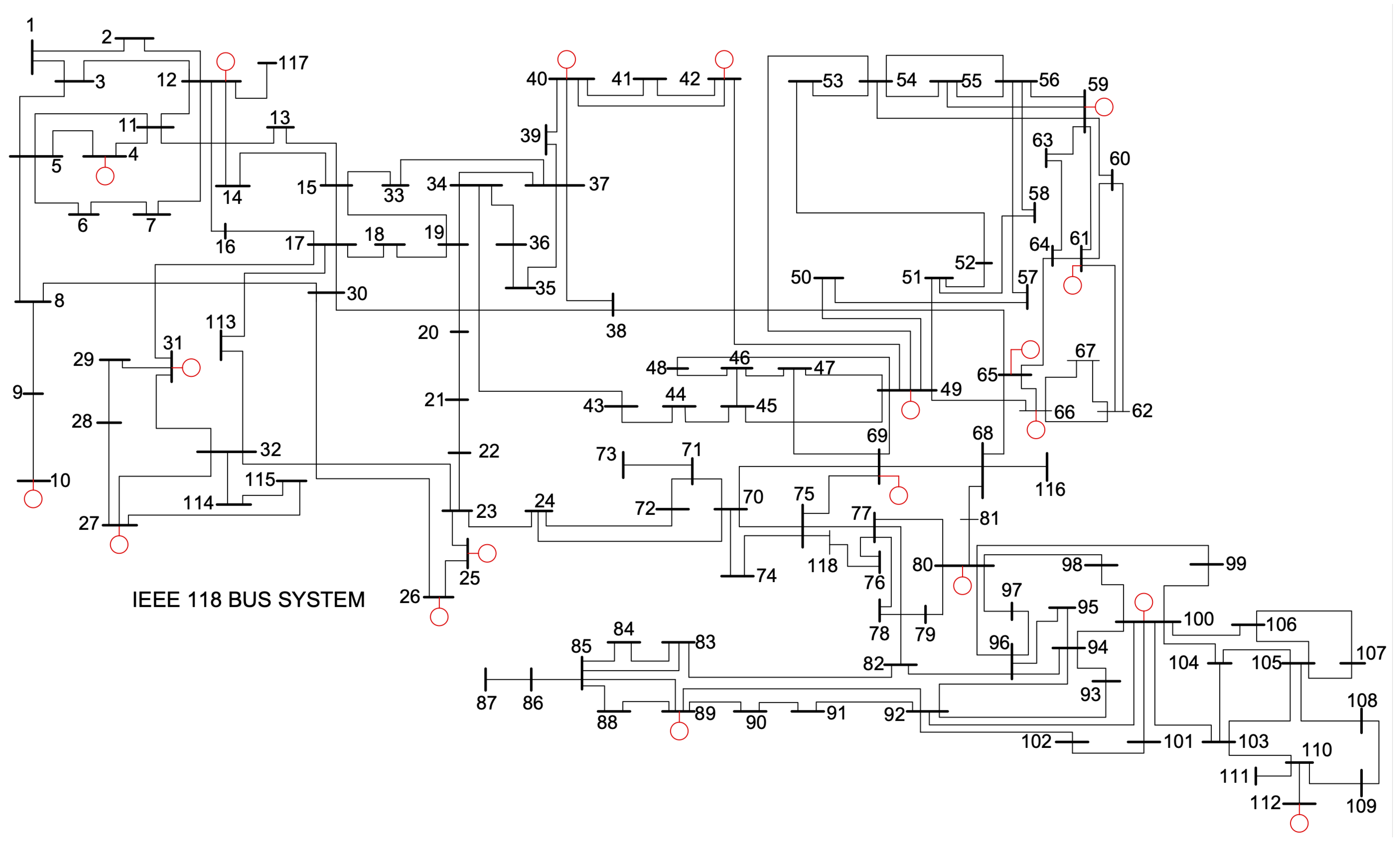
The assessment of the EKF algorithm’s efficiency using the nodal redundancy method was conducted on a MacBook Laptop (Apple’s M1 chip, featuring an eight-core GPU, 8 GB of memory, and 5 GHz, with an 866 Mbps maximum physical data rate). Simulations were performed on the IEEE 118-bus system as proposed in [24,31]. Test cases were prepared using an observable heuristic approach. The MATPOWER package was implemented to perform state estimation using the MATLAB platform. The processing time and the mean square error (MSE) of the estimated states shown in Equation (25) were used to evaluate the efficiency of the partitioning method applied to distributed estimation.

$$MSE=\sum _1^n\frac{{\left(x_i-{\widehat{x}}_i\right)}^2}{n}$$

(25)

For measurement errors, a random component was added to the load flow. In all simulations, it was assumed that the error was independent and followed an identically distributed Gaussian distribution (iid). In

Table 1. Variance of the measurement systems.

Type of Measure	Variable	Values
Voltage	${\mathit{\sigma }}_{\mathrm{V}}^2$	0.01
Power injection ${\mathit{P}}_{\mathit{i}}+j{\mathit{Q}}_{\mathit{i}}$	${\mathit{\sigma }}_{\mathrm{I}}^2$	0.015
Power flow ${\mathit{P}}_{\mathit{i}\mathit{j}}+j{\mathit{Q}}_{ij}$	${\mathit{\sigma }}_{\mathrm{F}}^2$	0.02

, the variance values of the measurement systems are presented, and

Table 2. Number of measurements in the IEEE118 bus system.

V	Injection P	Flow P	Injection P	Flow P	Number of Measurements
59	56	134	56	134	439

provides the type and number of measurements. Additionally, Figure 7 displays the schematic of the IEEE118 system.

4.1. Nodal Grouping Process

In the simulation process, the IEEE 118-bus system needed to be configured to enable the application of distributed estimation. This allowed for an analysis of the EKF filter within the process. To partition the system, the concept of nodal redundancy was employed, as described in [24]. This approach involved the use of a BN consisting of seven measurements.

Table 3. Partitioning of the IEEE118 bus system.

	Area 1	Area 2	Area 3	Area 4	Area 5
Nodal Bus	8	49	70	80	100
Bus #	27	37	17	12	25
Measurement #	101	138	64	55	81

provides details regarding the characteristics of the subsystems based on this approach. The Figure 8 shows the distribution of nodes and measurements in each subsystem, as well as the value of localized redundancy.

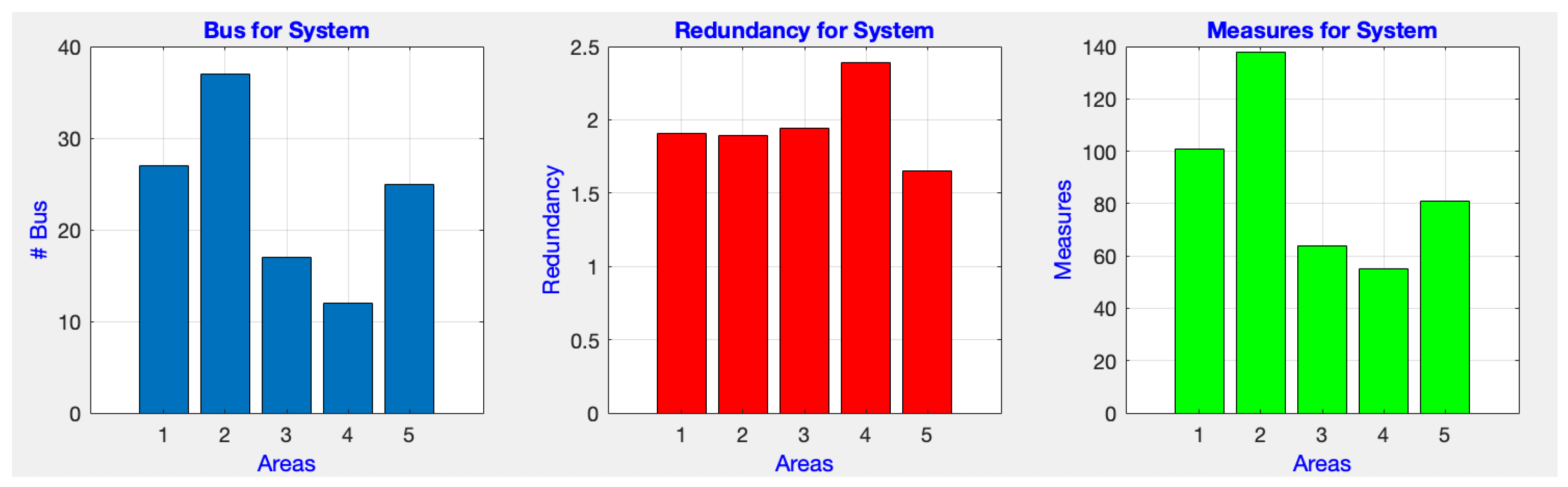
Having determined the physical conditioning of the system, for our simulation process, we established five subsystems, as shown in Figure 9. In each subsystem, we applied the iterative Kalman algorithm (IKF) for distributed estimation. Subsequently, the system was reconstructed to exchange information between the subsystems through their physical links.

In the Algorithm 1, a parallel process was employed to assess the a priori state and the gain matrix. During the update stage, information was exchanged across boundaries, facilitating the determination of the EPS state vector.

Algorithm 1 EKF distributed algorithm

Subsystem$\left({\mathbf{Area}}_{\mathbf{i}}\right)$   $\mathbf{function}[X,GA,d_Y]={\mathbf{f}}_{EKF}(XoA,arK,cov{a}_m,W,rep,D_{m}ed,M_i,$ $\mathbf{select} \mathbf{area} Are{a}_i\subset System-IEEE118$  $\mathbf{for}t=1,areas$   $X_{\mathbf{oA}}\leftarrow \{t:1=nbarras\}$  $cdemQK\left(i\right)\leftarrow \mathbf{for} \mathbf{i}=1,nbus$  $cdemPK\left(i\right)\leftarrow \mathbf{for} \mathbf{i}=1,nbus$   $d_Q\left(mat{V}_{iV}\right)\leftarrow \mathbf{for} iV=1,length\left(ma{t}_V\right)$   $d_P\left(mat{V}_{iV}\right)\leftarrow \mathbf{for} iV=1,length\left(ma{t}_V\right)$  $cdemQK\left(i\right)\leftarrow \mathbf{for} \mathbf{i}=1,nbarras$   $\mathbf{while} \mathrm{ek}>0.05\&\&\mathrm{iter}<30$  $[\mathbf{HX},{\mathbf{J}}_{\mathbf{i}},\mathbf{varVT}]=funHX({\mathbf{M}}_{\mathbf{i}},{\mathbf{mat}}_{\mathbf{Y}},\mathbf{xp})$  ${\mathbf{h}}_{\mathbf{x}}\leftarrow evaluacion(nbA,\mathbf{dVT},\mathbf{HX})$  ${\mathbf{H}}_{\mathbf{J}}\leftarrow funHJT({\mathbf{J}}_{\mathbf{i}},\mathbf{xp},{\mathbf{M}}_{\mathbf{i}},{\mathbf{mat}}_{\mathbf{Y}},\mathbf{varVT})$  $Gan{K}_i\leftarrow P_{ke}·H_J^T{(H_J·P_{ke}·H_J^T+c_m)}^{-1}$for $i=1,areas\leftarrow$ Profit Matrix  ${\mathbf{delta}}_{\mathbf{X}}\leftarrow \mathbf{GanK}·({\mathbf{D}}_{\mathbf{m}}-{\mathbf{h}}_{\mathbf{x}})$   $X(:,iter)=\mathbf{Xp}+\mathbf{GanK}\ast ({\mathbf{D}}_{\mathbf{m}}-{\mathbf{h}}_{\mathbf{x}}-{\mathbf{H}}_J·(\mathbf{Xp}-\mathbf{Xpos}(:,iter-1)))$  return $\mathbf{xp},\mathbf{GA},\mathbf{dY}$   Priori$\left({\mathbf{X}}_{\mathbf{oA}}\right)$  ${\mathbf{d}}_Y\leftarrow {({{\mathbf{H}}^{\mathbf{T}}}_{JT}·\mathbf{W}·{{\mathbf{H}}^{\mathbf{T}}}_{JT})}^{-1}\mathbf{W}·({\mathbf{D}}_{\mathbf{m}}-{\mathbf{h}}_{\mathbf{x}})$  $\mathbf{GA}\leftarrow ({{\mathbf{H}}^{\mathbf{T}}}_{JT}·\mathbf{W}·{\mathbf{H}}_{JT})$  return $\mathbf{X}\leftarrow \mathrm{State} \mathrm{vector}$

In the evaluation of the EKF applied to nodal redundancy, two scenarios were developed by considering the variation of injected powers in the system for which power flow data were available. To analyze the performance, a centralized weighted least squares (WLS) estimator, centralized EKF, and distributed estimator under the Kalman filter model were applied. The results are presented below.

4.2. Low Variation of $P_i+j{Q}_i$ in the Injected Power Balance

In a preliminary scenario, a variation of $5\%$ was considered as an input parameter in the power balance between an operation state T and $T+t$.

Table 4. Mean squared error (MSE) $minJ\left(x\right)={\sum }_1^n\frac{{\left(x_i-{\widehat{x}}_i\right)}^2}{n}$.

Iteration	EKF Distributed	EKF	WLS
0	0	0	0
1	5542.89	278.73	134,696.61
2	173.27	79.32	44.95
3	71.57	48.77	41.57
4	48.56	43.02	41.7
5	43.20	41.87	41.57
6	41.95	41.87	41.57

presents the values of the minimum mean square error (MSE) within the estimation process applied to the IEEE118 system.

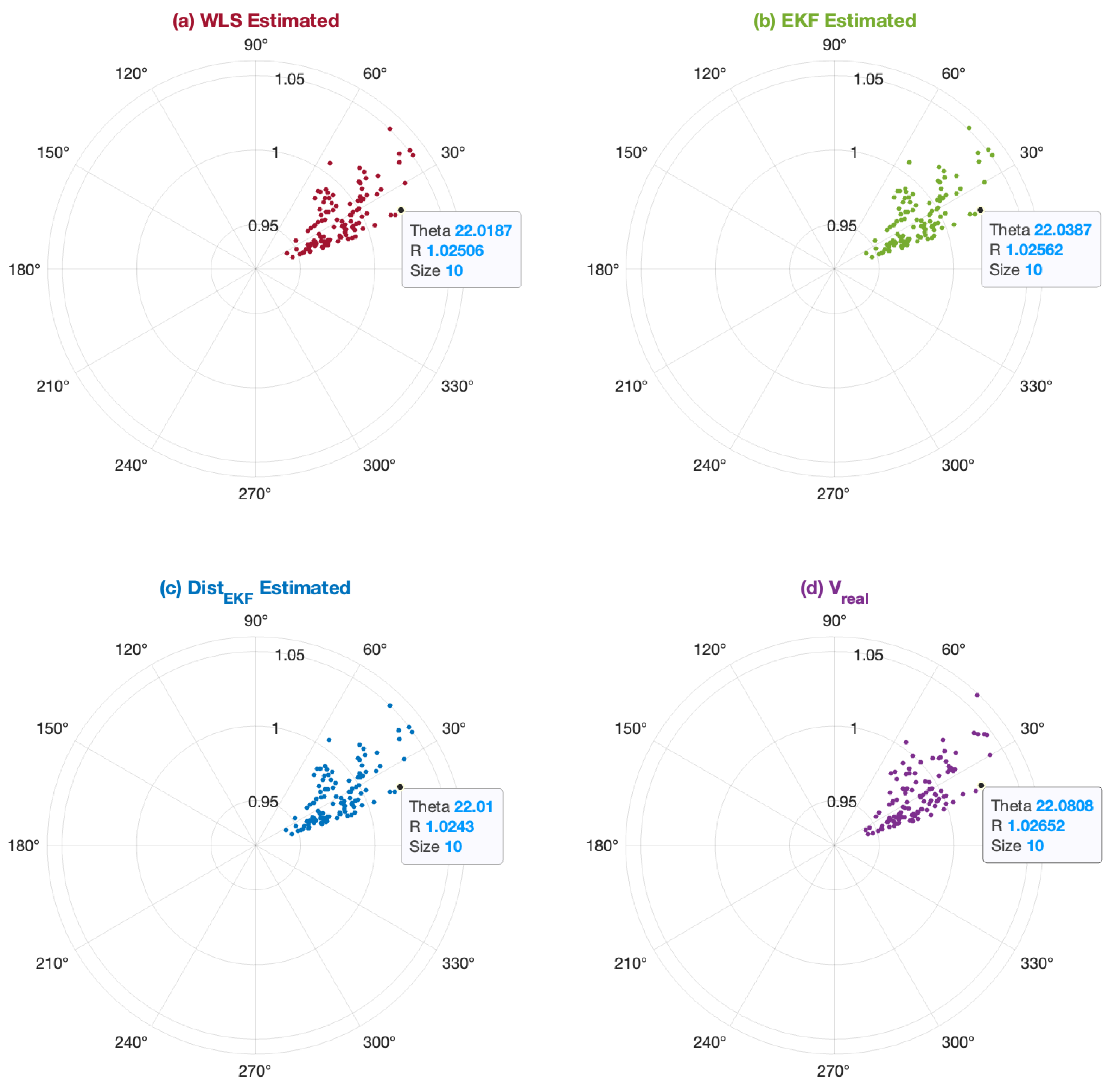
In Figure 10, the behavior of the voltage phasors applied in the proposed analysis scenario is depicted. This was achieved through the application of three estimation processes: two centralized methods, namely, WLS and EKF, and the third one through a distributed process using the nodal partition method, which leverages the mathematical model of the EKF estimator. The figure also presents the actual voltage phasors of the system during its operation. The points determine the voltage $V_i$ and its angle ${\theta }_i$. It can be observed that the concentration of the estimated state vector values exhibited a pseudo-symmetry, where no significant variation between the methods was noted. This was due to the insignificance of the power balance variation.

Similarly, to undertake a sensitivity analysis among the estimation methods, the estimated error in the system measurement set between real and estimated values in the estimation process was considered. This relationship is presented in Figure 11, where a similarity in concentration can be observed. However, in the distributed method, a higher concentration of error was observed.

In

Table 5. Computational processing time [min].

WLS Estimator	EKF Estimator	Distributed Estimator
11.61	14.30	20.03

, the time used within the estimation process is presented, comparing the centralized and distributed methods. This demonstrates the computational burden that the process utilized for the applied methods.

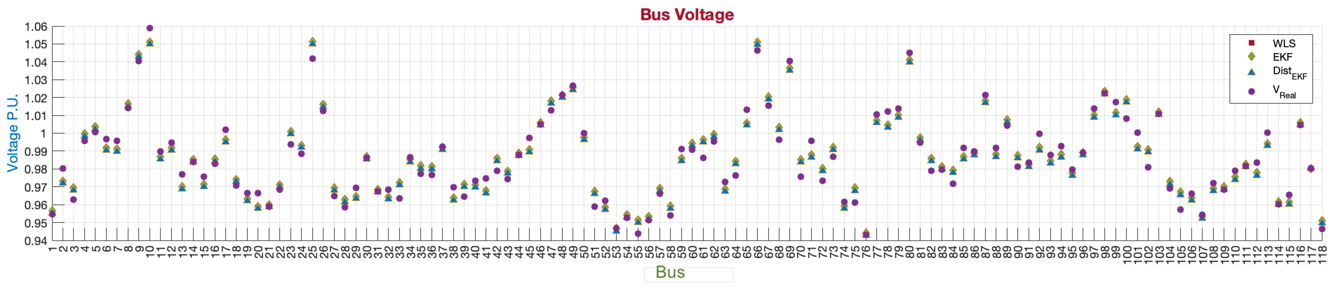
In Figure 12, the voltage values at each of the 118 buses of the IEEE118 system are presented. In all estimation processes, the resulting voltages closely approximated the real values, which is a consequence of a slow change in the system dynamics between one operating point and another.

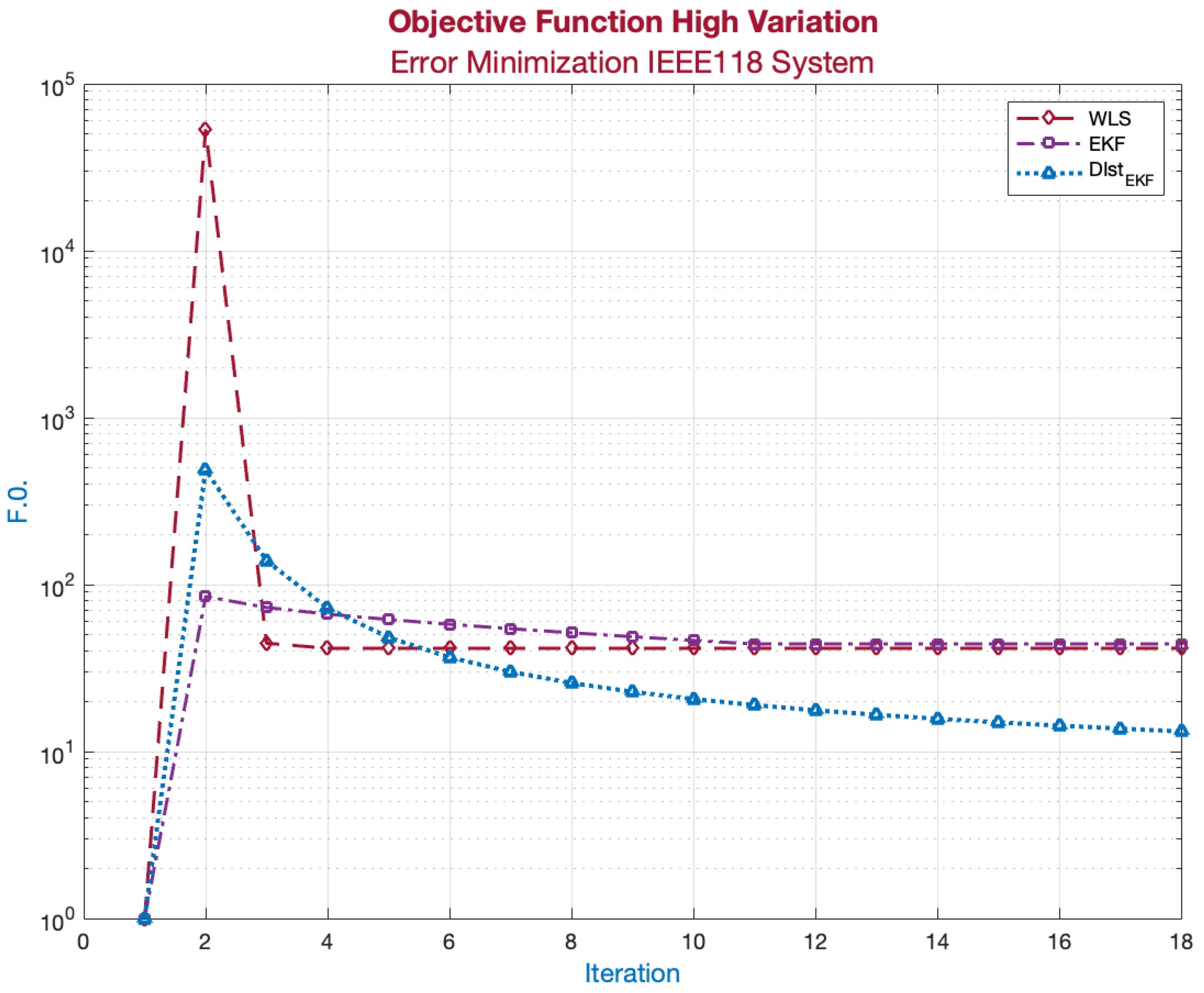
4.3. High Variation of $P_i+j{Q}_i$ in the Injected Power Balance

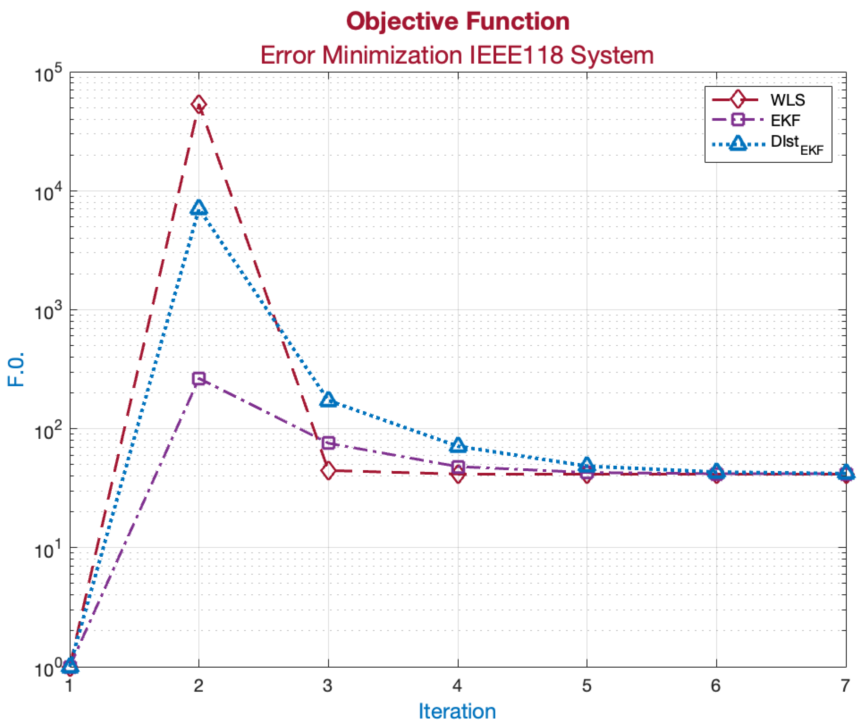
In the following Figure 13, the behavior of the objective function of the applied estimation methods is presented. Their convergence approximates a local solution of the state vector.

In this second case, focusing on the power balance deviation, the performance of both the centralized and distributed Kalman filters is analyzed. It was considered that the system exhibited a $10\%$ variation between two operating points. The considerations for this modeling are described as follows:

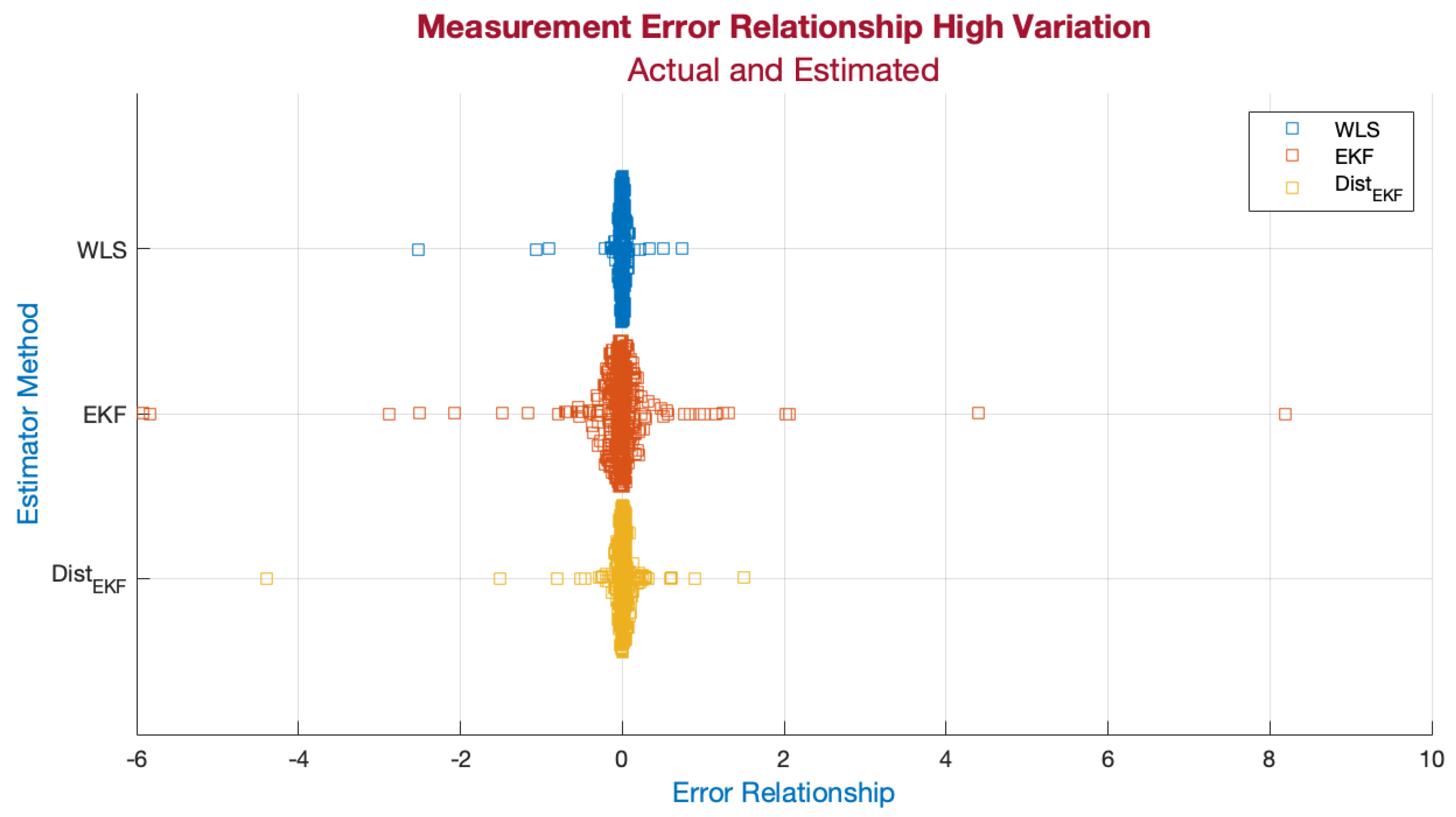
Under high variation in the power balance deviation of the system, a greater concentration of measurement errors was observed, as depicted in Figure 14, compared with the low-variation case. The difference in dispersion was notable, with it being lower in the distributed estimator than in both the centralized EKF and WLS.

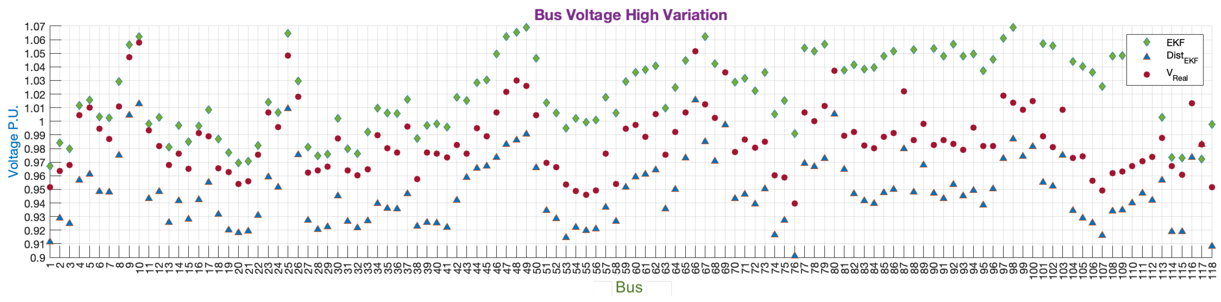
In Figure 15, the voltage magnitudes at each bus of the system are depicted for both centralized and distributed estimation processes. The estimated values closely tracked the real voltage value in both cases. However, the presence of an error could lead to misinterpretations of the system’s state.

Table 6. Comparison of MSE between centralized EKF and distributed EKF.

Iteration	EKF	EKF Distributed
0	487.31	84.88
1	138.89	72.92
2	72.27	66.58
3	48.27	61.81
4	36.70	57.87
5	30.04	54.47
6	25.76	51.46
7	22.79	48.77
8	20.63	46.31
9	18.98	44.07
10	17.67	44.07
11	16.61	44.07
12	15.72	44.07
13	14.96	44.07
14	14.30	44.07
15	13.72	44.07
16	13.20	44.07

presents the MSE results for each iteration. In the distributed estimation process, convergence was achieved by iteration 4, whereas in the centralized EKF, convergence occurred by iteration 9. However, in the distributed approach, although the result was improved, it required a longer processing time, as reflected by the higher number of iterations where the error decreased.

Similarly, comparing the scenario for centralized and distributed estimation through the implementation of the Kalman filter in both processes, it can be inferred from Figure 16 that the distributed approach converged faster to a local optimum. However, within the simulation, it also required a greater number of iterations to define another optimum that improved the values of the state vector. This indicates the need for a longer convergence time, rendering the application of the distributed EKF unable to provide a response within the time frame required by the system operator for decision-making in the operation of the electrical power system (EPS).

5. Discussion

The importance of applying the Kalman filter as an estimator lies in its ability to model systems beyond linearity, unlike the weighted least squares (WLS) estimator. However, it is crucial to consider various factors in this process, such as the reliability of results, not only of the state vector but also of the measurements represented by the set of nonlinear equations; processing time, which provides insight into the system’s state; and the identification of erroneous measurements that, due to communication processes, may skew the state vector results and lead to misinterpretations.

This study aimed to determine the reliability of a nonlinear filter, such as the extended Kalman filter (EKF), within a distributed estimator framework, employing the nodal redundancy model. This model creates subsystems to apply the Kalman filter within the process.

In the a priori stage of the filter process, the power balance variation between two operating points was considered as a starting point, which was then applied in the subsystems. Subsequently, in the a posteriori stage and during the reconstruction process, information regarding the boundaries between subsystems was considered and involved a set of measurements. During this stage, the model was iterated to determine the estimated state vector, incorporating the control metric, namely, the mean squared error (MSE).

Following this developmental stage and based on the results obtained in simulated cases, the application of another Bayesian filter described in the literature, such as the unscented Kalman filter (UKF), will be explored. Additionally, the analysis within this investigation will focus on evaluating its performance under the conditions utilized in this article.

6. Conclusions

The study underscores the pivotal role of Kalman filtering in nonlinear system estimation, highlighting its superiority over traditional techniques like weighted least squares (WLS). This capability becomes critical in environments characterized by nonlinearity or dynamic variations.

Emphasis is placed on meticulous consideration of several factors during the estimation process. These factors encompass the robustness of outcomes, encompassing both state vector reliability and measurement fidelity in the context of nonlinear equations. Moreover, meticulous identification of erroneous measurements, particularly in communication-prone settings prone to transmission errors, assumes paramount importance.

The study focuses on a rigorous evaluation of the Extended Kalman Filter’s (EKF) reliability within a distributed estimator framework leveraging the nodal redundancy model. This evaluation transcends mere state vector accuracy, extending to the efficacy of the entire estimation process, especially in complex or multi-variable scenarios.

The methodology employed is described, encompassing both a priori and a posteriori stages of the filtering process. This entails considering power balance variation between operational points, integrating information about subsystem boundaries, and utilizing control metrics such as the mean squared error (MSE). These stages ensure a thorough evaluation of the effectiveness and precision of the estimation process.

Looking ahead, the study sets forth a path to explore alternative Bayesian filters such as the nonlinear Kalman Filter (UKF). This exploration seeks to compare and evaluate the filter’s performance under conditions similar to those studied, potentially sparking new insights and methodologies in nonlinear system estimation.

In future research, the study will investigate the performance of the UKF filter and assess the influence of boundary information between subsystems. This analysis aims to understand the effects and find an alternative that ensures optimal performance without significantly increasing processing time.