Novel Self-Organizing Probability Maps Applied to Classification of Concurrent Partial Discharges from Online Hydro-Generators

Abstract

In this paper, we present an unprecedented method based on Kohonen networks that is able to automatically recognize partial discharge (PD) classes from phase-resolved partial discharge (PRPD) diagrams with features of various simultaneous PD patterns. The PRPD diagrams were obtained from the stator windings of a real-world hydro-generator rotating machine. The proposed approach integrates classification probabilities into the Kohonen method, producing self-organizing probability maps (SOPMs). For building SOPMs, a group of PRPD diagrams, each containing a single PD pattern for training the Kohonen networks and single- and multiple-class-featured samples for obtaining final SOPMs, is used to calculate the probabilities of each Kohonen neuron to be associated with the various PD classes considered. At the end of this process, a self-organizing probability map is produced. Probabilities are calculated using distances, obtained in the space of features, between neurons and samples. The so-produced SOPM enables the effective classification of PRPD samples and provides the probability that a given PD sample is associated with a PD class. In this work, amplitude histograms are the features extracted from PRPDs maps. Our results demonstrate an average classification accuracy rate of approximately 90% for test samples.

1. Introduction

Partial discharges (PDs) are localized electrical currents that occur within the insulation system of high-voltage equipment without causing a complete failure of the insulation. These discharges are typically caused by inhomogeneities in the insulation dielectric material, leading to localized intensification of the electric field and subsequent breakdown. PD activity is often characterized by the generation of electrical pulses, electromagnetic radiation, acoustic emissions, and chemical byproducts like ozone [1,2,3]. Understanding the type and location of PD is crucial for assessing the condition of the insulation and predicting potential failures. PD monitoring is a crucial measure regarding predictive maintenance procedures on rotating machines in the electric power industry [4]. PD-monitoring-driven maintenance goals are mainly concerned with keeping the generators operating properly and ultimately avoiding catastrophic events which could lead to machine loss. However, PD diagnostic methods rely on human experts to analyze the data, which is time consuming, costly, and limits the amount of data that can be inspected. While PD monitoring has standard methods to assess insulation health, real-world voltage distortions can affect how discharge responses appear [5]. Furthermore, multiple classes of discharges can emerge simultaneously [6]. To overcome those challenges, machine learning algorithms have been proposed for PD classification, which would enable automated and efficient diagnostics.

Traditional machine learning algorithms, like support vector machines and artificial neural networks, have been used for PD classification.

Table 1. Methods (and their characteristics) used for hydro-generator PD recognition in the literature and the method proposed in this work.

Papers	Algorithms	Classification Probabilities	Input Features and Metrics
Krivda and Gulski [7]	Kohonen	No	Pulse count and amplitude distributions
Araújo et al. [8]	MLP	No	Histograms (Normalized)
Lopes et al. [9]	CNN	No	Histograms
Pardauil et al. [10]	K-means and RF	No	Histograms
Zemouri et al. [11]	GAN	No	2D PDA
Zemouri et al. [12]	Deep Learning	No	Edge Detection Filter, Statistical Features
Dang et al. [13]	Supervised contrastive learning (SCL)	No	t-distributed stochastic neighbor embedding (t-SNE)
This work	SOPM (novel)	Yes (concurrent PD classification)	Amplitude Histograms, sample-neuron distances in the space of features

provides a comparative overview of various methods used for PD recognition in hydro-generators, including our proposed approach. Each row is associated with a different research paper, and the columns highlight key aspects of the methods: algorithms employed, whether the probability of a PRPD map being associated with a PD class is calculated (statistics), and the input features used for PD recognition.

Krivda and Gulski implemented Kohonen neural networks for classifying PDs [7]. The Kohonen networks demonstrated varying classification accuracies based on the number of neurons in the Kohonen layer. The best obtained Kohonen network had 12 neurons in the Kohonen layer, and it achieved a classification accuracy of 90% for two PD classes. Araújo et al. [8] implemented a Multilayer Perceptron (MLP) algorithm, employing normalized histograms as input features and achieving a single PD source classification accuracy of 94.4%. Lopes et al. [9] utilized Convolutional Neural Networks (CNNs) with real-world hydro-generator data with histograms as input, resulting in an accuracy of 89.44% for single-source PD classification. Pardauil et al. [10] combined k-means and Random Forest (RF) algorithms with data mining and clustering, using histograms as input, and achieved an accuracy of 99% for classifying single PD sources. In [11], Zemouri et al. developed an approach using a Generative Adversarial Network (GAN) and a Variational Autoencoder (VAE) to enhance the representativeness of individual PD sources in the VAE latent space with 2D Partial Discharge Analyzer (PDA) data as input. Zemouri et al. [12], introduced a multifaceted approach, utilizing the U-Net model for source isolation, Deep Learning models for PD recognition, and a novel decision-making technique for output classification. Real-world hydro-generator data analysis yields a 87% gap source detection accuracy and accuracy rates of 91%, 95%, 96%, and 94% for Internal, Corona, Slot, and Delamination single-source PDs. In [13], a method for fault diagnosis in high-voltage equipment using supervised contrastive learning (SCL) with data augmentation is proposed and applied to PRPD data collected using UHF sensors. SCL achieves a classification accuracy over 96% for single-class PRPDs. Note that in [8,9,10,11,12,13], PRPD maps with only one well-defined PD pattern each were considered and, therefore, accuracy rates tended to be around 90%.

The complex nature of PD patterns necessitates sophisticated analysis techniques. As noted in [5], real-world voltage distortions can significantly alter the appearance of discharge responses, making interpretation challenging. Furthermore, the simultaneous occurrence of multiple PD classes, as observed in [2,14,15,16], further increases the difficulty of accurate classification. These complexities highlight the limitations of traditional PD diagnostic methods relying on human expertise and underscore the need for automated and robust solutions. Prior research has explored various machine learning algorithms for PD classification, including Kohonen neural networks [7], Multilayer Perceptrons [8], and Convolutional Neural Networks [9]. However, these methods predominantly focus on single-class PD patterns, limiting their applicability in real-world scenarios where multiple PD sources are often present. Therefore, in this work, we aim to overcome these limitations by proposing the self-organizing probability map (SOPM) algorithm, a novel approach combining Kohonen networks with statistical analysis to enable accurate classification of PRPDs with concurrent features of several classes by mapping the input data into a two-dimensional space where we assign classification probabilities to each neuron in the map. The algorithm is trained on a set of PRPDs acquired from real-world hydro-generator machines and it can accurately classify PRPD maps not contained in the training set regardless of whether they contain single- or multiple-class features, providing a more comprehensive diagnostic tool than traditional methods. The paper is structured as follows: Section 2 presents a background on partial discharges, including their occurrence in hydro-generators and signal processing; Section 3 has information about our PD data set obtained from on-line hydro-generator; Section 4 contains a review of Kohonen Self-Organizing Maps; In Section 5 and Section 6, we describe the proposed SOPM method; In Section 7, SOM and SOPM results are presented and discussed; and, finally, in Section 8, conclusions are drawn.

2. Background on Partial Discharges

Partial discharges are electrical events that occur in non-uniform regions within an insulating material of high-voltage equipment. They happen when an electric field exceeds the material’s dielectric strength without leading to a complete insulation breakdown [17]. In simpler terms, partial discharges can be thought of as localized electrical discharges that do not fully bridge the gap between phase conductors and the ground. PDs are primarily initiated by imperfections within the insulating material. These imperfections can manifest as gas bubbles, voids, inclusions of foreign materials, or surface irregularities [1,17,18]. When the applied voltage reaches a certain threshold, these imperfections can act as initiation sites for electrical discharges.

As significant markers of insulation degradation in electrical equipment, PDs are particularly relevant to rotating machines such as motors and generators [1,10,17,18,19,20]. Specifically, in the context of synchronous generators, which are the focus of this work, approximately $60\%$ of the defects can be attributed to failures of electrical insulation of stator windings [21]. Three common types of PD found in rotating electrical machines are slot discharges, internal discharges and end-winding discharges, each with distinct characteristics and implications [1,2]. Slot discharges occur in the air gap between the stator core and the conductive slot portion of the winding, often arising from poor contact or damage to the conductive coating. Internal discharges occur within the main insulation, typically due to voids or delamination caused by manufacturing defects or aging. End-winding discharges, on the other hand, occur on the surface of the insulation in the end-winding region, often resulting from contamination, damaged field grading materials, or inadequate installation procedures; while internal discharges and slot discharges pose a greater risk of insulation failure due to their erosive nature, end-winding discharges are generally less critical but can accelerate aging under certain conditions [1]. Distinguishing between these PD types is essential for accurate diagnosis and effective mitigation strategies [3]. According to the IEC60034-27-2 standard [1], it is possible to derive characteristic patterns representing specific defects from PD measurements. Consequently, tracking PDs is associated with monitoring the progression of equipment defects. Accurate identification and classification of PDs are crucial for preventive maintenance, allowing issues to be rectified before they result in catastrophic equipment failures. Electromagnetic signals of PDs are typically detected and monitored using specialized techniques that measure discharge currents, propagating electromagnetic waves or visible light pulses generated by the discharges.

In order to correlate PD phenomenon and its causes, it is necessary to verify the pattern(s) formed by the discharges [1]. After measuring the current pulses and reference signals, a Phased Resolved Partial Discharge (PRPD) map is created to visualize the pattern formed by the discharges and then link it to a possible defect type. PRPD maps correlate amplitude q of the PDs, their occurrence phase $\varphi$ and the quantity n of PDs [1,17,22]. Thus, PRPDs are a fundamental tool for distinguishing the phenomena among the various types of defects that can give rise to PDs (see [1,23]).

Figure 1 shows PRPD maps for various PD classes of defect obtained from a real hydro-generator: Slot Discharge (S), Internal Void (InV), Internal Delamination (InD), Delamination Between Conductor and Insulation (DCI) and corona discharge (C). For the same reasons given in [8], samples of the internal cavity (InV) and internal delamination (InD) classes were merged into a new InV/InD class, and the samples of slot (S) and corona (C) classes were combined into a new S/C class in the PRPD database. Furthermore, Figure 1f,g show examples of PRPDs with simultaneous features of multiple patterns: InD+DCI and InD+S, respectively, as one can see by comparing Figure 1f with Figure 1c,d and by examining in detail Figure 1g along with Figure 1a,c.

Each pixel color within a PRPD map corresponds to a quantity of PD peaks sharing the same amplitude and phase, i.e., it maps PD count. Prior to PRPD assembling, data preprocessing is applied to filter out discharges with amplitudes near zero, leaving only representative discharge peaks, resulting in a region devoid of discharges termed as the gap.A collection of uninterrupted, connected discharges (non-white pixels) forms what is referred to as a cloud of discharges in PRPD maps. Discrimination between different DP patterns hinges on an examination of cloud shapes and their symmetry around the gap zone. In this work, the measurements of electrical signals from hydro-generator PDs were conducted using capacitive couplers, which were employed to separate the fast PD signals from the 60 Hz signal. The electric current pulses were recorded over multiple cycles of the 60 Hz voltage signal, from which the phase is used for composing PRPDs.

2.1. Partial Discharges in Hydro-Generators

In hydroelectric generators, partial discharges (PDs) are a common occurrence within the stator bar insulation system. These discharges are categorized based on their specific location within the bar and are typically classified as slot discharges, internal discharges, and end-winding discharges.

Slot discharges (S) primarily arise as a result of the generator’s vibration, which, over time, erodes the semi-conducting layer which should avoid high electric field gradients on the surfaces of stator bars [17]. Once the semi-conducting layer is sufficiently damaged, PDs emerge. Slot PDs generate a characteristic PRPD pattern, as is seen in Figure 1a. The PD pattern in Figure 1a is distinguished from other PD types by its positive- and negative-voltage discharge clouds with triangular shapes, with the positive-voltage cloud being more prominent than the negative one. This kind of voltage-level asymmetry has been referred to as positive-voltage asymmetry in [24].

Internal discharges, which occur within the insulation layers of stator bars, can be further classified into three distinct categories: internal void (InV), internal delamination (InD), and delamination between conductor and insulator (DCI).

InV discharges primarily result from the formation of air bubbles during the manufacturing process of the bars [10]. These discharges exhibit a unique Phase-Resolved Partial Discharge (PRPD) pattern characterized by rounded and symmetrical discharge clouds, as illustrated by Figure 1b.

On the other hand, InD discharges are manifested as detachments or elongated cavities located between the insulation layers. The PRPD pattern of InD discharges features symmetrically arranged triangular clouds around the gap zone (refer to Figure 1c).

As the name suggests, DCI discharges occur in proximity to the copper conductor of the bars. These faults are typically initiated by overheating, which subsequently leads to the detachment of the insulation layers. The PRPD pattern associated with DCI discharges is distinguished by a negative-voltage cloud that surpasses the positive-voltage cloud in amplitude, thereby resulting in a negative-voltage asymmetry, as is seen in Figure 1d.

Finally, corona discharges (C) occur when the electric field between end-winding and nearby surfaces becomes stronger than the surrounding air’s dielectric strength, thus ionizing the air. An arc between stator bar and the air is formed, which is responsible for the bright glow and buzzing noises characterizing typical corona discharges. Preventing corona discharges requires careful design of end-winding and adjacent surfaces, primarily by avoiding high electric fields near conductors, which are usually mitigated by using anti-corona sleeves. Once corona sleeves are damaged, corona PDs emerge. A typical PRPD pattern of corona discharges is characterized by positive-voltage cloud asymmetry. PRPD corona clouds tend to have rounded shapes, as seen in Figure 1e.

2.2. PRPD Denoising and Feature Extraction

In the process of PD class recognition, filtering of PRPD maps is a critical step [25]. When PD measurements are conducted in an operating generator, its stator is subjected electrical, mechanical, and thermal stresses, which account to noise addition to signal measurements [8,24]. Therefore, the filtering step is essential for attenuating noise and interference, thereby increasing recognition rates.

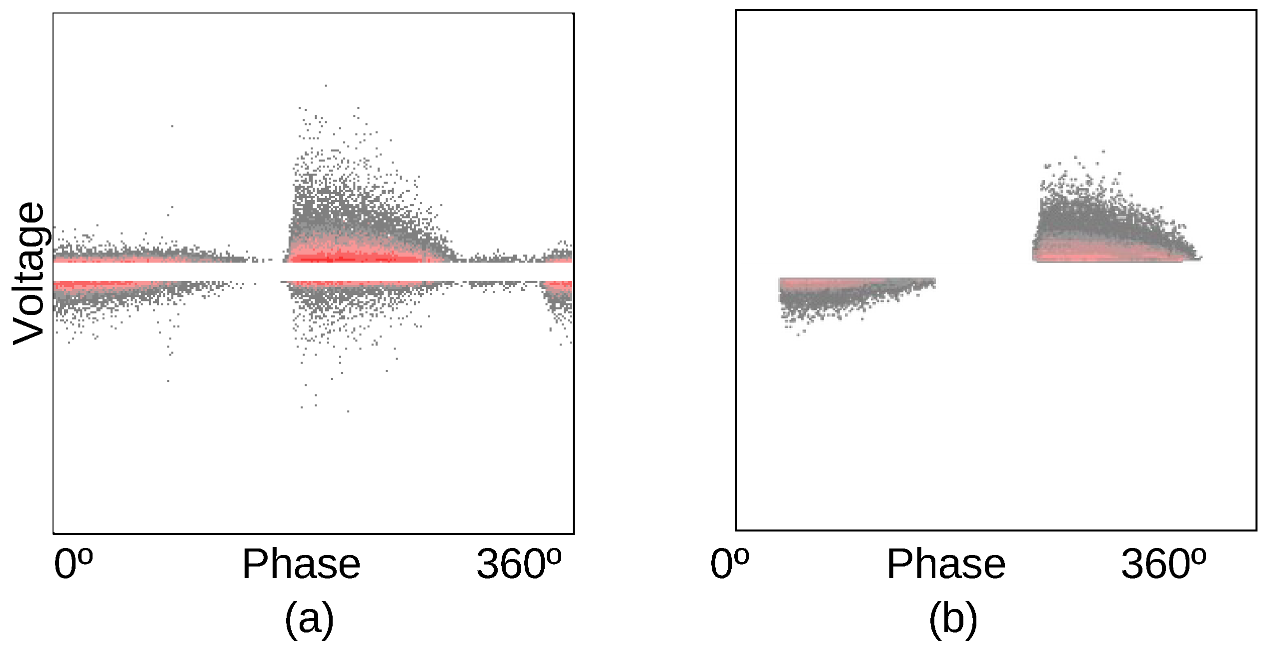
In this study, we utilize the PRPD image-based PD denoising algorithm proposed in [8]. This filtering algorithm treats PRPD maps as images and it is capable of eliminating low-density PD clouds or PD peaks not linked to large clouds (usually associated with noise) and, furthermore, it is able to remove non-dominant PD clouds present due to cross-talk. Those noise sources are commonly observed in online hydro-generators. As illustrated in Figure 2a,b, the application of the denoising algorithm significantly increases the possibility of automatic recognition of PD cloud shapes in PRPD patterns and, therefore, improves the overall PD recognition process.

In order to increase the DP classification rates, in addition to filtering, it is crucial to minimize the number of dimensions of the inputs by providing the network exclusively indispensable attributes (features) to properly group PD samples by classes in the space of features while keeping classes properly separated. The feature extraction method described in [8] was adopted in this paper. As PRPDs contain positive- and negative-voltage PDs, for each polarity, two sets of histograms are generated [8] resulting in four distinct normalized histograms: two phase histograms (one for positive voltage and the other for negative voltage) and two voltage histograms (also each one for positive and negative PD polarity). Therefore, amplitude histograms are used as classification features in this work.

3. The Data Set Obtained from the On-Line Hydro-Generators

The data set used in this study consists of online-measured PDs from hydro-generators at the Tucuruí and Coaracy Nunes hydroelectric power plants, both situated in north region of Brazil. The employed electrical measurement procedures are based on traditional capacitive sensing systems. The capacitors are distributed over the stator bars of each hydro-generator.

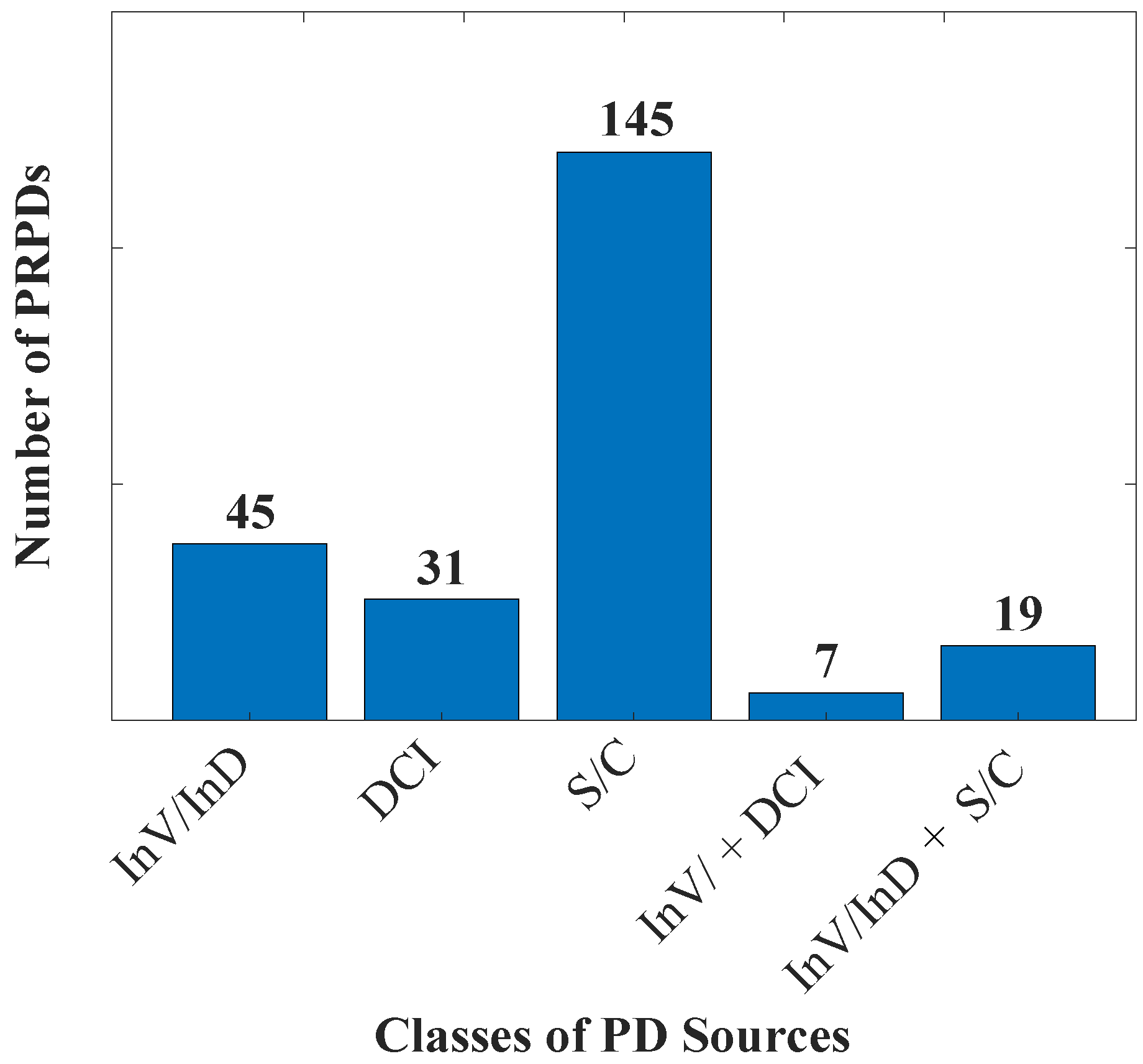
PD patterns were manually labeled by an expert professional following the PD classes outlined in IEC 60034-27-2 [1] (internal void (InV), internal delamination (InD), delamination between conductor and insulation (DCI), slot (S), corona (C), surface and gap discharges). This study does not encompass samples of surface PDs or gap PDs classes. Figure 3 displays the quantities of samples in the database for each class.

4. Review of Kohonen Self-Organizing Maps (SOMs)

Kohonen self-organizing maps or networks, originally proposed by T. Kohonen [26], consist of a type of unsupervised neural network trained via competitive learning that produce lower-dimensional discrete representations of the training samples, i.e., maps. Therefore, Kohonen networks consist of an arrangement of neurons with weights. The neural arrangements typically have one, two, or three dimensions mapping the higher-dimensional space of features defining the input samples [27]. While preserving the data’s topographic structure [28], Kohonen maps are particularly useful for tasks like clustering, data visualization, and dimensionality reduction.

Since sample groups are usually complex to visualize and analyze in the original high-dimensional space of features, the input samples are grouped on the maps based on their topographic similarities [29]. Therefore, Kohonen SOMs are commonly assembled in two dimensions. In a Kohonen SOM, each neural node $i=1,2,\dots ,zy$ in the network has assigned a weight vector ${\mathbf{w}}_i=[w_{i1},w_{i2},\dots ,w_{im}]$ with the same number of dimensions m as input sample $\mathbf{x}=[x_1,x_2,\dots ,x_m]$. Quantities z and y are the total numbers of lines and columns of the neural map. During the training procedure, weight vectors are progressively adjusted to properly clustering samples with similar features set. The Euclidean distances from $\mathbf{x}$ to all weight ${\mathbf{w}}_i$ vectors are computed. The neuron with a weight vector closer to the input vector is called the Best Matching Unit (BMU).

In Figure 4a, the arrangement of samples and neurons in the a didactic two-dimensional space of features is shown (note that, frequently, $m>3$). It can be observed that BMU (red neuron) is the closest neuron to $\mathbf{x}$ and, therefore, it has the highest similarity level with the input sample $\mathbf{x}$. Figure 4b,c show, respectively, BMU on the SOM map (with neural weights and input sample) and the SOM map with each neuron labeled as the class of its exciting samples with foregrounded BMU.

Once the BMU is identified, its weight vector and its neighboring nodes are updated to be closer to the input vector, as Figure 5 illustrates in the didactic two-dimensional space of features. Over a sufficient number of iterations, the map will organize itself in such a way that sub-areas will be formed and associated with a specific characteristic (i.e., a set of features) of the training samples.

4.1. Training SOM Networks

SOM networks can be trained using a sequential algorithm [27]. A single input sample is used to update the weights of the neurons per training epoch t (iteration). Training SOMs involves initialization, sampling, similarity matching, update of weights of neurons, and repetition of the process while the map changes. As mentioned earlier, the goal of training is to update the weights of neurons to approximate the feature vectors representing N samples in such a way that each region of the map is able to gather similar samples.

The first key step towards achieving this goal is to find the neuron ${\mathbf{w}}_c\left(t\right)$ closest to the current input sample ${\mathbf{x}}_j\left(t\right)$. The neuron ${\mathbf{w}}_c\left(t\right)$ is referred to as the BMU (Best Matching Unit) to ${\mathbf{x}}_j\left(t\right)$. The index c of the neuron ${\mathbf{w}}_c$ is defined by using

$$c\left(\mathbf{x}\left(t\right)\right)={\mathrm{argmin}}_i\Vert \mathbf{x}\left(t\right)-{\mathbf{w}}_i\left(t\right)\Vert ,$$

(1)

where $\Vert .\Vert$ is the norm operator, and the function $\mathrm{argmin}$ returns the index of the neuron that minimizes the norm [30]. Then, weights of all neurons are updated by using

$${\mathbf{w}}_i(t+1)={\mathbf{w}}_i\left(t\right)+\alpha \left(t\right)h_{i,c\left(\mathbf{x}\right(t\left)\right)}\left(\mathbf{x}\left(t\right)-{\mathbf{w}}_i\left(t\right)\right),$$

(2)

where $\alpha \left(t\right)$ is the learning rate at iteration t, and $h_{i,c\left(t\right)}$ is the neighborhood function regarding neurons with indices i and c (BMU) at iteration t.

In (2), both $\alpha \left(t\right)$ and $h_{i,c\left(t\right)}$ are functions that decay over epochs. This is necessary for achieving convergence of the training process. In this work, the learning rate $\alpha \left(t\right)$ is calculated using

$$\alpha \left(t\right)={\alpha }_0{e}^{-t/\tau },$$

(3)

where $\tau$ is a constant used to adjust the decay level of the learning rate and ${\alpha }_0$ is the initial value of $\alpha \left(t\right)$. The neighborhood function is computed in this work employing

$$h_{i,c\left(\mathbf{x}\right(t\left)\right)}=exp\left(-\frac{d_{i,c\left(\mathbf{x}\right(t\left)\right)}^2}{2{\sigma }^2}\right),$$

(4)

in which $d_{i,c\left(\mathbf{x}\right(t\left)\right)}$ is the distance between the winning neuron c and the excited neuron i, and $\sigma$ is the neighborhood radius function, given by

$$\sigma \left(t\right)={\sigma }_{0}exp\left(-t/\tau \right),$$

(5)

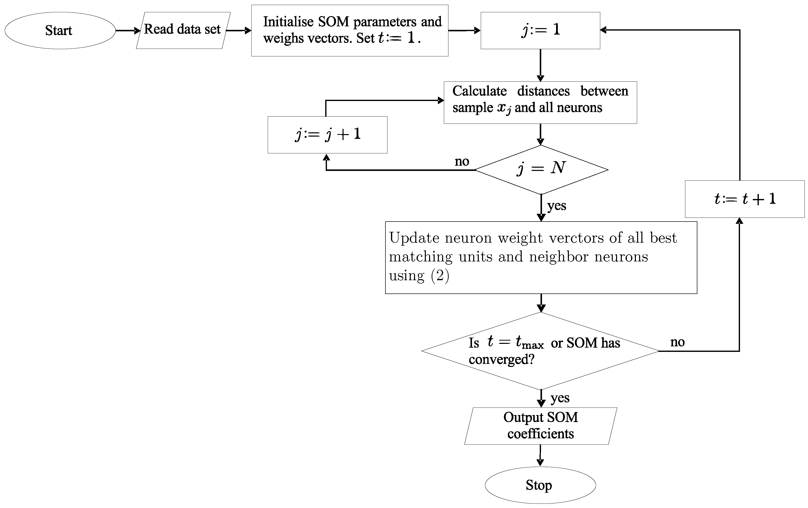
where ${\sigma }_0$ defines the initial neighborhood radius [27]. The neighborhood range (or radius) determines the number of neurons that will be updated along with the BMU. Therefore, we may say that Kohonen self-organizing maps employ a neighborhood function to facilitate the formation of topologically ordered representations of high-dimensional data. This function, often modeled using a Gaussian distribution as given in (4), determines the extent to which the weight update of the winning neuron influences neighboring neurons during the learning process. The distance between neurons $d_{i,c\left(\mathbf{x}\right(t\left)\right)}$ dictates the strength of this influence, with closer neurons experiencing a greater impact. Furthermore, Equation (5) introduces an exponential decay of the neighborhood radius $\sigma \left(t\right)$ over iteration index t. This decay ensures that the initial broad influence of the winning neuron is gradually reduced, eventually encompassing only the winning neuron itself. The combined effect of these mechanisms balances global order and local specialization within the SOM. During the early stages of learning, the large neighborhood radius promotes the formation of ordered clusters of neurons with similar properties in each cluster. As the learning progresses and the radius shrinks, fine-tuning of individual neuron weights allows for a more precise representation of the input data distribution. This kind of interplay between global and local updates contributes to the ability of SOM to effectively cluster complex high-dimensional data [27]. Finally, in Figure 6, we present a flowchart illustrating the employed training process of the SOM networks in this work.

4.2. Metrics for SOM Evaluation

In this work, we used two well-known metrics to evaluate SOM networks: the quantization error $Q_E$ and the topographic error $T_E$, which are derived in [27]. The quantization error $Q_E$ corresponds to the average of the Euclidean distances obtained between each input sample and its corresponding BMU. Thus, $Q_E$ is given by

$$Q_E={\displaystyle \frac{1}{N}}\sum _{j=1}^N\Vert {\mathbf{x}}_j-{\overline{\mathbf{w}}}_j\Vert ,$$

(6)

where N is the total number of samples and ${\overline{\mathbf{w}}}_j$ is the BMU of sample ${\mathbf{x}}_j$. The smaller the quantization error is, the closer the BMUs are to the input samples.

Topographic error $T_E$ is an important measure because it directly assesses how well the SOM preserves the topology of the input space. A low topographic error indicates that similar data points in the high-dimensional space are mapped to adjacent units on the map, thus suggesting appropriate topographic preservation. It is calculated by

$$T_E={\displaystyle \frac{{\sum }_{j=1}^{N}u\left(x_j\right)}{N}},$$

(7)

where $u\left(x_j\right)=0$ if the BMU and the second closer neuron to the sample are adjacent and $u\left(x_j\right)=1$ otherwise.

In this work, all training processes have been executed until convergence, i.e., until minimization of $Q_E$ and $T_E$ have been achieved. This ensures that the resulting self-organizing maps are optimally tuned to accurately reflect the underlying structure and distribution of the input data, maximizing the efficacy of the model for subsequent analysis, interpretation, and novel developments.

5. The Novel Self-Organizing Probability Maps (SOPMs)

In this section, we present a new method for automatic classification of simultaneous PDs based on Kohonen networks, which has been named the self-organizing probability map (SOPM). For each class with index k, the classification probability labels of a neuron with index i are determined by the average Euclidean distance $D_i^k$, calculated in the space of features between ${\mathbf{w}}_i$ and the n samples from class k that are closer to that neuron. Thus, the closer a neuron is to a given class in the space of features, the higher is the probability of that neuron to be associated with that class.

5.1. Calculation of $D_i^k$

Thinking of a class as a group of points, i.e., samples, that are geometrically close to each other in the space of features, we can define the distance between ${\mathbf{w}}_i$ and a class k as the average of the distances between the neuron ${\mathbf{w}}_i$ the n samples nearest to it. Therefore, mathematically one has

$$D_i^k={\displaystyle \frac{1}{n}}\sum _{j=1}^n{d}_{i,j}^k,$$

(8)

in which $d_{i,j}^k$ corresponds to the Euclidean distance between neuron ${\mathbf{w}}_i$ and the j-th sample of class k, which is given by

$$d_{i,j}^k=\Vert {\mathbf{w}}_i-{\mathbf{x}}_j^k\Vert .$$

(9)

For each class k and neuron ${\mathbf{w}}_i$, distances $d_{i,j}^k$ given by (9) are previously sorted in ascending order and in that way accessed as j is increased from 1 to n when calculating $D_k^i$ by employing (8).

A visual representation of the process of obtaining $D_i^k$ is illustrated in Figure 7a, which shows samples of three distinct classes and neurons in a didactic two-dimensional space of features ($x_1$ and $x_2$ are the features). With $n=2$, distances $d_{i,j}^k$ measured from neuron ${\mathbf{w}}_i$ (the red hexagon) to samples j of each class k are being calculated. It is notable that, although ${\mathbf{w}}_i$ is not positioned in a specific group of samples of any class, that neuron is very close to the edge of the group of samples of class 1, indicating that ${\mathbf{w}}_i$ is more likely to be associated with that specific class. This can also be seen in Figure 7b, which shows lines connecting ${\mathbf{w}}_i$ to positions in space of features at averaged coordinates calculated using the $n=2$ closer samples to ${\mathbf{w}}_i$ from each class k. The so-defined connecting lines measure $D_i^k$. Finally, Figure 7c shows distances $D_i^k$ on a distance d-axis for k ranging between 1 and 3.

5.2. Calculation of Classification Probabilities $P_i^k$

Classification probabilities $P_i^k$ are calculated and assigned to each neuron ${\mathbf{w}}_i$. $P_i^k$ is the probability of a neuron with the index i being associated a class indexed by k. The smaller $D_i^k$, the higher $P_i^k$.

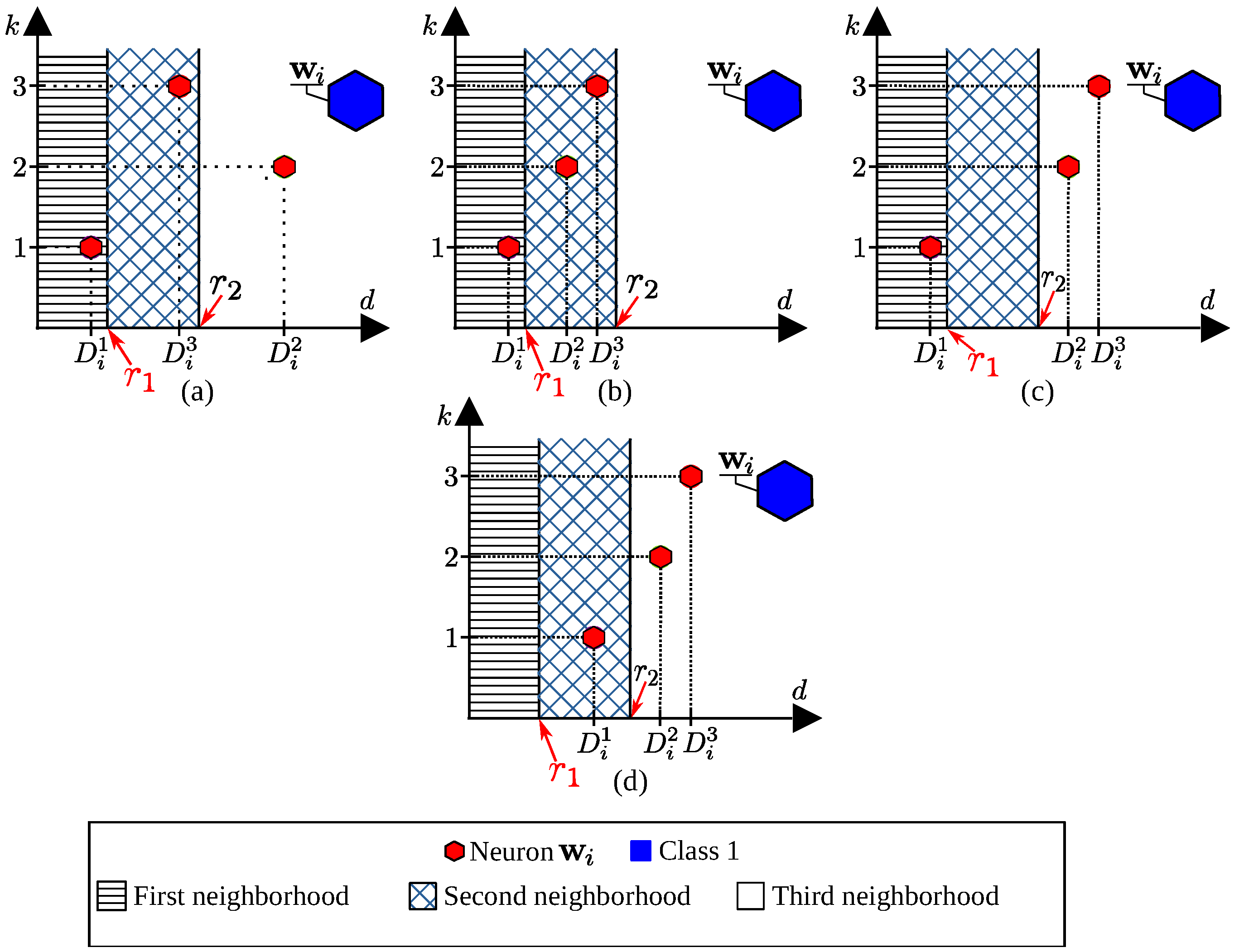
The calculation of classification probabilities is performed by defining neuronal neighbor regions, as Figure 8a illustrates. The first neuronal neighborhood comprises distances $D_i^k$ from zero to $r_1$ (the first neighbor threshold which measured from neuron ${\mathbf{w}}_i$). This first neuronal neighborhood region can be understood as the space contained within a hypersphere of radius $r_1$ in an m-dimensional space of features. If there is at least one class k with $D_i^k\le r_1$, all other classes will be assigned a zero classification probability at neuron ${\mathbf{w}}_i$. The second neighbor threshold $r_2>r_1$ is also measured from neuron ${\mathbf{w}}_i$. Thus, the second neuronal neighborhood lies between the hypersphere of radius $r_1$ and the hypersphere of radius $r_2$, as Figure 8b illustrates. The second neighborhood region has influence on neuronal probabilities if $D_k^i>r_1,\forall k$. Finally, the third neuronal region encompasses the entire hypervolume outside the hypersphere with radius $r_2$. Classes with average distances greater than $r_2$, such as in Figure 8c for the class with $k=2$, have their association with neuron ${\mathbf{w}}_i$ disregarded, i.e., $P_i^2=0$. The numeric values of $r_1$ and $r_2$ are obtained by using the optimization algorithm Cuckoo-GRN [31], applied to maximize average accuracy rate of the SOPM system.

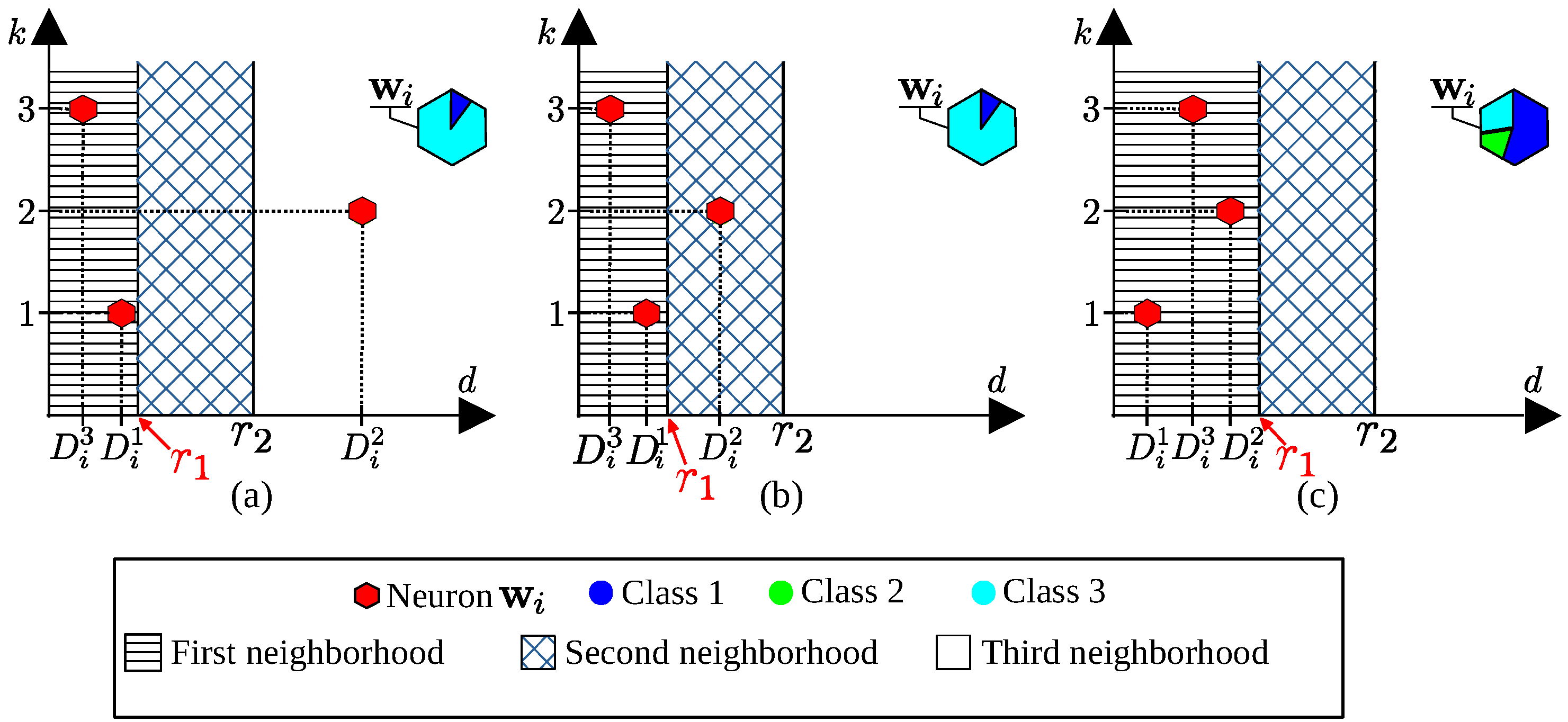
In Figure 9, Figure 10 and Figure 11, we present detailed illustrations of the neural positions on the distance axis, accompanied by thresholds $r_1$ and $r_2$, and the resulting proposed probability neural representation. In Figure 9, the neuron ${\mathbf{w}}_i$ is showcased in instances where $P_i^1=100\%$. Figure 9a–c depict scenarios where $D_i^1\le r_1$, ensuring a classification probability of 100% for class 1. In the case of Figure 9d, the neuron remains associated with class 1, with $D_i^2>r_2$ and $D_i^3>r_2$ but specially because $r_1<D_i^1\le r_2$. The blue color represents neurons associated with class 1, and the classification probabilities are proportional to the areas covered by each color in the probability neural representation.

In Figure 10, the neuron ${\mathbf{w}}_i$ is presented in scenarios where it is associated with multiple classes. Figure 10a,b illustrate situations where the neuron is linked to classes 1 and 3 due to $D_i^1\le r_1$ and $D_i^3\le r_1$, and in Figure 10c, it is associated with classes 1, 2, and 3 since $D_i^k<r_1$ for all k. The colors blue and cyan in Figure 10a,b represent the classes 1 and 3, while in Figure 10c, the colors blue, green, and cyan signify associations with classes 1, 2, and 3. The classification probabilities are indicated by the respective colored areas in the probability neural representation, providing a comprehensive visualization of the neuron’s associations with multiple classes under different distance conditions.

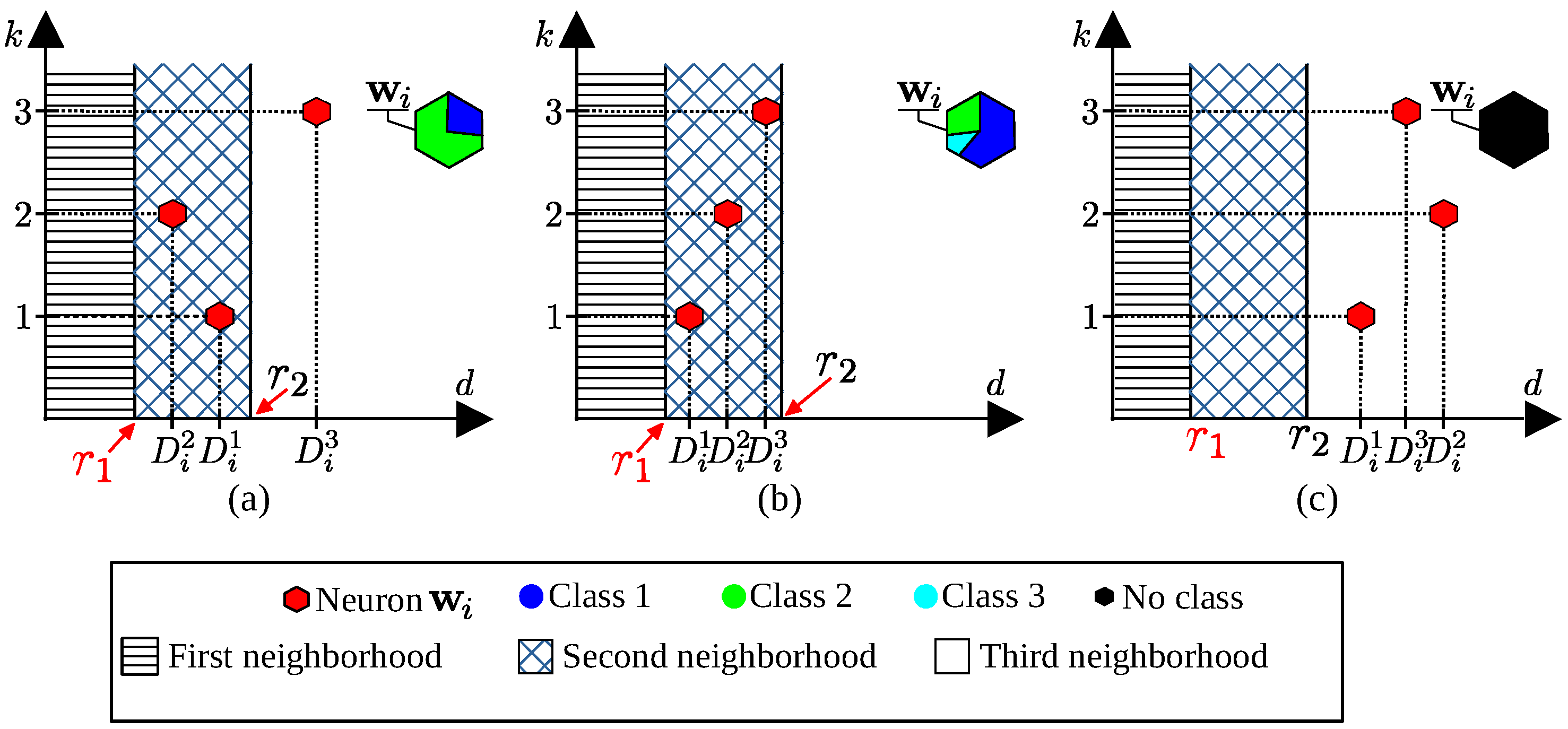
In Figure 11, the neuron ${\mathbf{w}}_i$ is depicted in three distinct scenarios, each illustrating cases where it is associated with more than one class or to no class. In Figure 11a, the neuron is linked to classes 1 and 2 because its distance to class 1, i.e., $D_i^1$, falls within the range $[r_1$, $r_2]$, the distance $D_i^2$ also falls within the same range, while the distance to class 3 $D_i^3$ exceeds $r_2$. Figure 11b portrays a scenario where the neuron is associated with classes 1, 2, and 3. This occurs because the distances to all three classes, $D_i^1$, $D_i^2$, and $D_i^3$, are all within the range $[r_1,r_2]$. In contrast, Figure 11c represents a case where the neuron is not linked to any class, as its distances $D_i^k$ for all classes exceed the threshold $r_2$. The black color has been used for representing neuron ${\mathbf{w}}_i$ in that case.

Once visual representations of ${\mathbf{w}}_i$ in various scenarios have been shown and discussed, along with illustrations of its associated classification probability cases, mathematical definitions can be given. For cases where there is only one class k within the first neighborhood region of ${\mathbf{w}}_i$, or when all classes have distances greater than $r_1$ and only a class k has its distance to ${\mathbf{w}}_i$ smaller than $r_2$, the probability $P_i^k=100\%$ for that class. Otherwise, we might have smaller classification probabilities. We may thus write

$$P_i^k={\delta }_i^k\times 100\%,\mathrm{if}\sum _{k^{\prime }=1}^s{\delta }_i^{k^{\prime }}=1\mathrm{or}\sum _{k^{\prime }=1}^s{\delta }_i^{k^{\prime }}=0$$

(10)

and

$$P_i^k=\left(1-{\displaystyle \frac{{\delta }_i^k}{{\displaystyle \sum _{k^{\prime }=1}^s}{\delta }_i^{k^{\prime }}}}\right)\times 100\%,\mathrm{otherwise}.$$

(11)

For cases in which multiple classification probabilities are associated with ${\mathbf{w}}_i$, one employs (11). In (10) and (11), ${\delta }_i^k$ is an auxiliary parameter used for probability calculation, which is obtained from the analysis of the cases illustrated in Figure 9, Figure 10 and Figure 11 and it is given by

$$\begin{array}{c}\hfill {\delta }_i^k=1,\mathrm{if}f(D_i^k,r_1)=1\mathrm{and}\sum _{a=1}^{s}f(D_i^a,r_1)=1\mathrm{or}f(D_i^k,r_2)=1\mathrm{and}\\ \hfill \sum _{a=1}^s[f(D_i^a,r_1)+f(D_i^a,r_2)]=1,\end{array}$$

(12)

$${\delta }_i^k={\displaystyle \frac{D_i^k}{r_1}},\mathrm{if}f(D_i^k,r_1)=1\mathrm{and}\sum _{a=1}^{s}f(D_i^a,r_1)>1,$$

(13)

$${\delta }_i^k=\frac{D_i^k-r_1}{r_2-r_1},\mathrm{if}f(D_i^k,r_2)=1\mathrm{and}\sum _{a=1}^{s}f(D_i^a,r_1)=0\mathrm{and}\sum _{a=1}^{s}f(D_i^a,r_2)>1$$

(14)

and

$${\delta }_i^k=0,\mathrm{otherwise}.$$

(15)

In (12)–(14), $f(D,r)$ is defined as

$$\begin{array}{c}\hfill f(D,r)=\left\{\begin{array}{cc}\hfill 1,\hfill & \hfill \mathrm{if}D⩽r\hfill \\ \hfill 0,\hfill & \hfill \mathrm{if}D>r.\hfill \end{array}\right.\end{array}$$

(16)

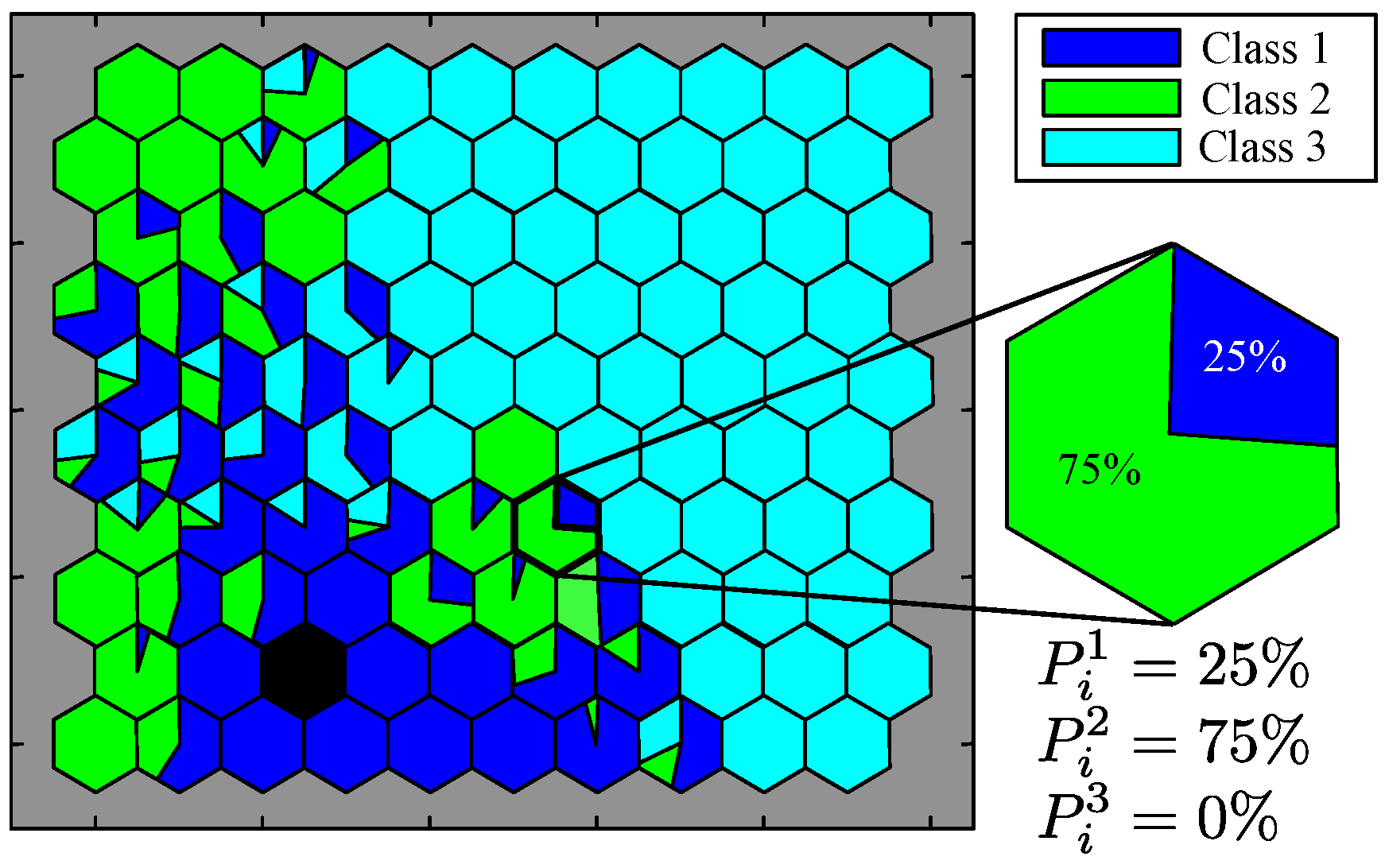
The parameter ${\delta }_i^k$ is computed based on the values of $D_i^k$ for each class considering the neighborhood thresholds $r_1$ and $r_2$. In the case where class k is within the second neighborhood region, i.e., $f(D_i^k,r_2)=1$, and all other classes are in the third neighborhood region, i.e., ${\displaystyle \sum _{a=1}^s}[f(D_i^a,r_1)+f(D_i^a,r_2)]=1$, ${\delta }_i^k$ is set to 1 for class k and 0 for other classes. Figure 9d illustrates such a case where only class 1 is in the second neighborhood region. Another scenario arises when the neuron is associated with multiple classes, indicating multiple class features may be present. For cases with more than one distance within the first neighborhood region, ${\delta }_i^k$ is set to $D_i^k/r_1$ for all classes within this region, i.e., $D_i^k$ is normalized by the first neighborhood radius $r_1$, and ${\delta }_i^k$ is set to 0 for other classes. Figure 10a–c exemplifies instances of such cases. For scenarios with multiple distances within the second neighborhood region and no class in the first region, ${\delta }_i^k$ is set to $\left(D_i^k-r_1\right)/\left(r_2-r_1\right)$ for relevant classes, i.e., $r_1$ is used as the zero distance and $D_i^k-r_1$ is normalized by $r_2-r_1$ (the effective distance threshold for this case) and ${\delta }_i^k$ is set to 0 for other classes. Figure 11a,b depict such cases, with Figure 11a showing a case with features of classes 1 and 3, and Figure 11b exhibiting a case with features of all classes. Note that $r_1$ is used as a referential distance value. Finally, neurons far enough from all classes, i.e., $D_k^i>r_2$ for all k, present a $0\%$ probability, as shown in Figure 11c and they are represented using the color black. Importantly, $P_i^k$ is determined by $D_i^k$, enabling the assignment of probabilities for neurons at class intersections, visually represented on the map by colored neurons with percentages indicated by the degree of color filling. Figure 12 illustrates an instance of the SOPM. Neurons are depicted as hexagons, with each color corresponding to a specific class. Notably, the inset highlighted neuron demonstrates probabilities for multiple classes, with a $75\%$ likelihood of association with class 2 and a $25\%$ probability for class 1.

6. The SOPM Algorithm

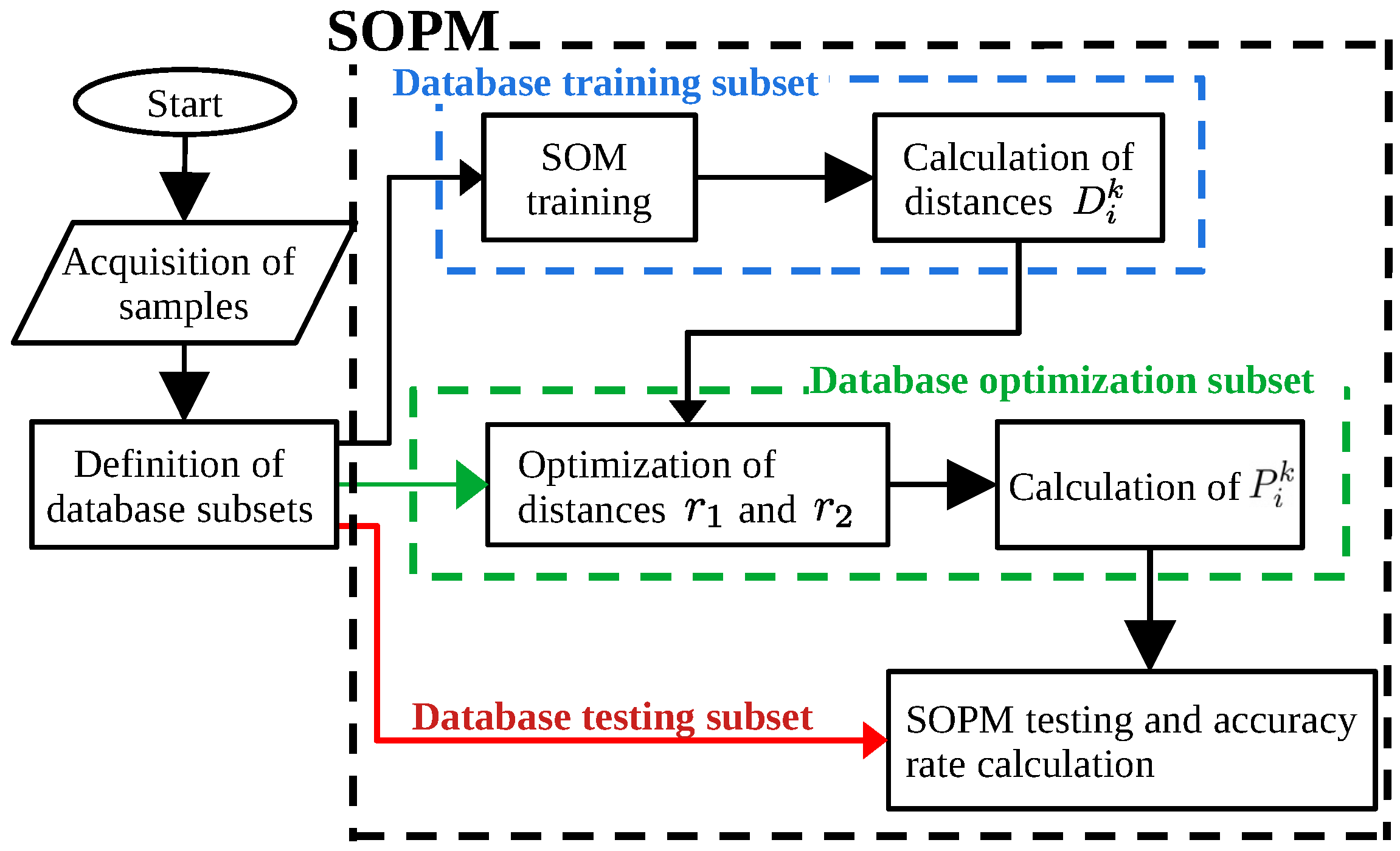
In this study, we employ the proposed SOPM method for the classification of partial discharge patterns obtained from online hydro-generator. The developed method is depicted in the flowchart presented in Figure 13. The flowchart delineates the SOPM processes into three distinct phases: training, optimization of $r_1$ and $r_2$, and testing of the SOPM.

In each phase of the algorithm, a specific sub-database is used to prevent the SOPM from over-specializing on the given samples. Thus, the database samples were distributed into three disjoint sub-bases: (1) the SOM network training sub-base, (2) the sub-base used for performing optimization of distances $r_1$ and $r_2$, and (3) SOPM testing sub-base.

The training sub-base, as the name suggests, is used to train the SOM network. In this sub-base, the chosen samples must be the most representative of each class, thus avoiding samples that may present dubious characteristics, i.e., features of more than one class. Exclusively samples with features of a single class each are used. The SOM training is an iterative process that aims to find the training parameters that best suit the input data (the training sub-base). The network is trained to simultaneously minimize the quantization error $Q_E$ and the topographic error $T_E$ of the Kohonen map, respectively, given by (6) and (7). In this process, different configurations of map size and $\tau$ values are tested. According to [32], the number of neurons should be from two to seven times the number of samples used in the training process. In this work, we have used the SOM neural network size $10\times 10$ and $\tau =2000$. The initial neighborhood parameter ${\sigma }_0$ was chosen in accordance to the SOM dimensions y and z, and it is given by ${\sigma }_0=\sqrt{y^2+z^2}$. The maximum number of epochs was set to $\mathrm{60,000}$ for all networks trained. This maximum number of epochs ensures the training convergence, i.e., the minimization of $Q_E$ and $T_E$ is assured.

After the SOM training stage, the optimization process of the distances $r_1$ and $r_2$ begins, aiming at maximizing the correct classification rates of the system, i.e., maximizing its accuracy. In this process, a great diversity of inputs is used, including multiple-class-feature samples, since it is in this stage that the probabilities $P_i^k$ will be defined. For performing optimization of the parameters $r_1$ and $r_2$, the algorithm Cuckoo-GRN [31] has been used with the goal of maximizing average accuracy of the SOPM system.

The calculation of the accuracy rate ${\overline{A}}_{\mathrm{cc}}$ is performed in a manner similar to what is performed in a conventional supervised network, that is, by comparing the network’s output with the targets of the samples. In the context of this study, the samples can be classified as associated with one or to multiple classes. The target is represented by a vector ${\mathbf{T}}_j=[t_j^1,t_j^2,\dots ,t_j^s]$ of zeros and ones, corresponding to the class(es) associated with the sample j. For instance, for a given sample labeled as class 1 in a problem with only three classes, we have a target vector ${\mathbf{T}}_j=[1,0,0]$. Therefore, if sample j is associated with classes 1 and 2, we would have ${\mathbf{T}}_j=[1,1,0]$.

Unlike conventional networks, which for classification problems always return a single possible class as a classification response, SOPMs can output probabilities for more than one class possibly associated with a given sample. Therefore, the calculation of the accuracy rate is performed differently depending on whether the neuron is associated with multiple classification probabilities or not. When a neuron excited by a given sample j has $P_i^k=100\%$ for a given class $1\le k\le s$, the accuracy rate for the referred sample is calculated by

$$A_{\mathrm{cc}}\left(j\right)={\displaystyle \frac{{\displaystyle \sum _{a=1}^s}[P_{c\left(j\right)}^a{t}_j^a]}{{\displaystyle \sum _{a=1}^s}{t}_j^a}},$$

(17)

where $c\left(j\right)$ is the BMU index for sample j. When the neuron excited by a given sample j presents probabilities associated with multiple classes, the classification accuracy for sample j is

$$A_{\mathrm{cc}}\left(j\right)=\sum _{a=1}^s[P_{c\left(j\right)}^a{t}_j^a].$$

(18)

Thus, the accuracy rate of the network is considered to be the average

$${\overline{A}}_{\mathrm{cc}}=\frac{1}{N}\sum _{j=1}^N{A}_{\mathrm{cc}}\left(j\right),$$

(19)

in which the sub-database of test samples are considered. Note that (19) is maximized while using Cuckoo-GRN for optimizing $r_1$ and $r_2$ with the optimization subset of samples.

7. Results and Discussion

In this section, the obtained results regarding application of SOM and of the proposed SOPM method for performing classification of PDs are shown and discussed. Single- and multiple-class-featured PRPDs are classified using the new SOPM method. For performing tests on the proposed method, we have trained a SOM network with neural dimensions of $10\times 10$, with $\tau =2000$, using single-class-featured PRPDs. Then, cuckoo-GRN optimization of thresholds $r_1$ and $r_2$ and calculation of SOPM classification probabilities $P_j^k$ have been conducted as previously described in this work.

7.1. SOM Classification Results

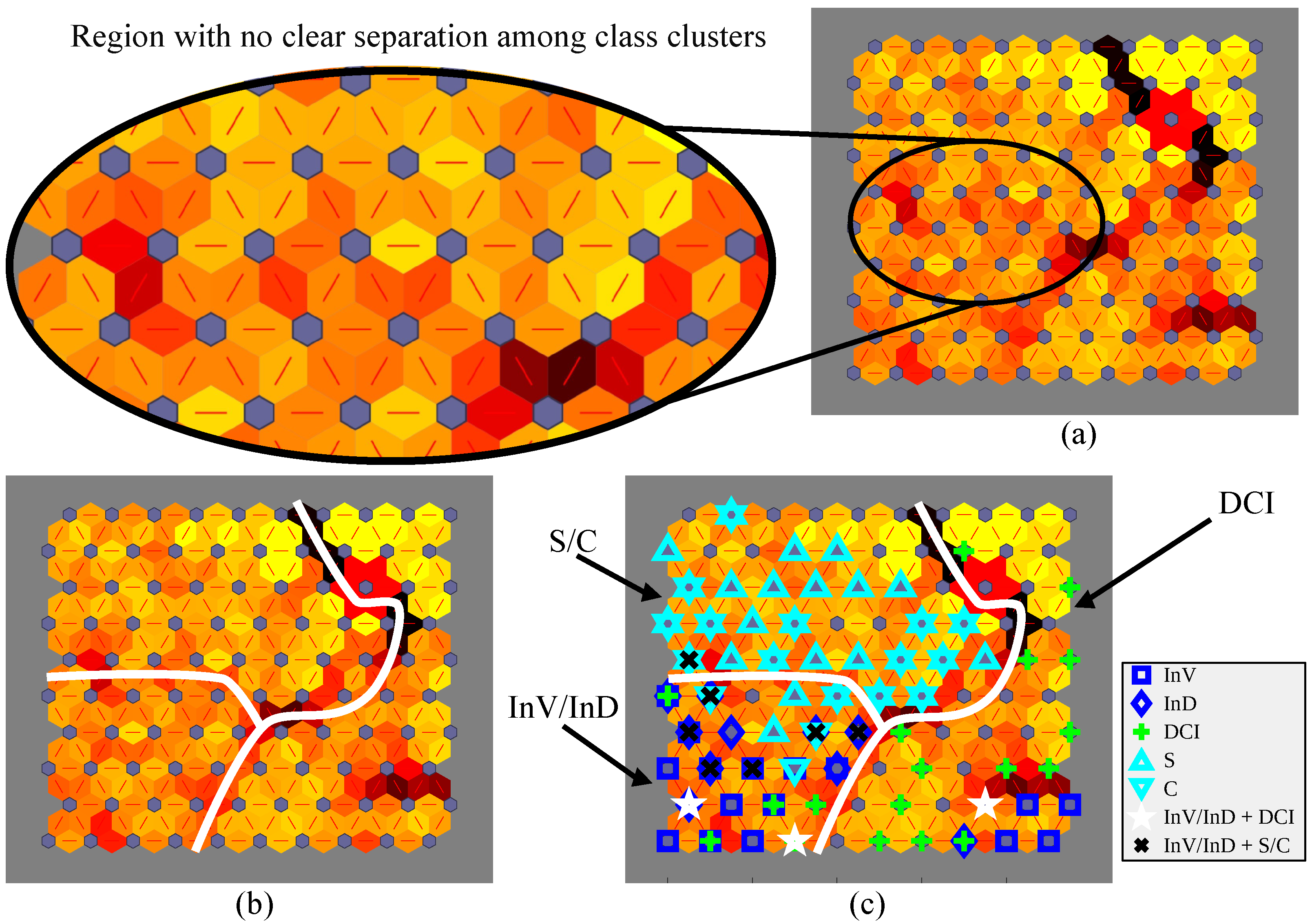
For the sake of comparison with the proposed SOPM method, we develop a simple sample classification method using the SOM network. In Figure 14a, our obtained $10\times 10$-SOM is shown, in which yellowish tones represent small distances among neurons, and orangish colors are associated with intermediate distances and red and darker colors indicate the greater distances among neurons. By observing Figure 14b,c, one notices that regions can be boundaried according to the samples classes exciting neurons, as specifically depicted in Figure 14c, thus forming discernible classification clusters. Class assignments to the so-formed clusters are made based on predominant sample classes within each neuron group [33], as shown in Figure 14c. Boundaries established among the classification regions are highlighted by the white lines in Figure 14b,c. Although it is possible to delineate clusters after the completion of the training phase, definition of boundaries remain ambiguous since the partitioning of the SOM network based on inter-neuronal distances depends on threshold values, which are subjected to human interpretation.

In

Table 2. SOM confusion matrix obtained using training samples, where bold values highlight correct classification rates.

True Class	Predicted Class
	Inv/InD	DCI	S/C
Inv/InD	80.00%	20.00%	0.00%
DCI	13.33%	86.67%	0.00%
S/C	13.33%	0.00%	86.67%

, the classification rates obtained to the training samples are shown. Accuracy assessment of the training data showcases rates ranging from 80.00% to 86.67%, slightly below the desirable threshold of 90%.

In order to classify multi-class-featured samples effectively, it is imperative that the network’s output comprises a combination of multiple classes. Nonetheless, the conventional self-organizing map architecture yields outputs corresponding to the predominant class of the activated neuron’s cluster. Consequently, it is unfeasible to classify multi-class-featured-samples solely relying on the SOM network. Consequently, to assess the efficacy and precision of the SOM map, exclusively single-feature samples from the test dataset were utilized. It should be noted that, as depicted in Figure 14c, multiple-class-featured samples are classified as one of the classes composing its multi-class features array. However, it is crucial to highlight that the multi-class samples were not included in the confusion matrix obtained for the test samples, which is seen in

Table 3. SOM confusion matrix obtained using single-class-featured test samples, where bold values highlight correct classification rates.

True Class	Predicted Class
	Inv/Ind	DCI	S/C
Inv/Ind	92.59%	7.41%	0.00%
DCI	53.85%	46.15%	0.00%
S/C	14.17%	0.00%	85.83%

. As one can see, the SOM network yielded inadequate accuracy rate, registering 46.15% for the PD class DCI.

7.2. SOPM Classification Results

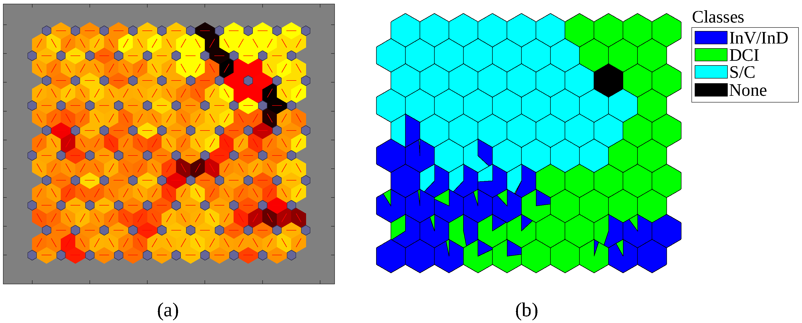
The obtained SOPM is shown in Figure 15b. We observe not just a clear neural division among the different classes, as shown by the single-colored neurons, but also transition regions among the areas associated with single-class samples. The transition regions, formed by neurons associated with multiple classes, are used for performing classification of multiple-class-featured samples, which tend to excite such neurons, and to estimate the respective classification probabilities of each sample exciting a given transition neuron. As previously described, classification probabilities are proportional to the areas filled with colors associated with each class.

In contrast to the SOPM, in obtained SOM map (Figure 15a), there is no obvious information on the classes of the samples that have excited each neuron, and much less on which class they are associated with. Those characteristics are intrinsic to SOM maps, even though it uses different shades of colors to delimit groups formed by neurons, where lighter colors represent small distances among neurons and darker colors represent larger distances in the space of features.

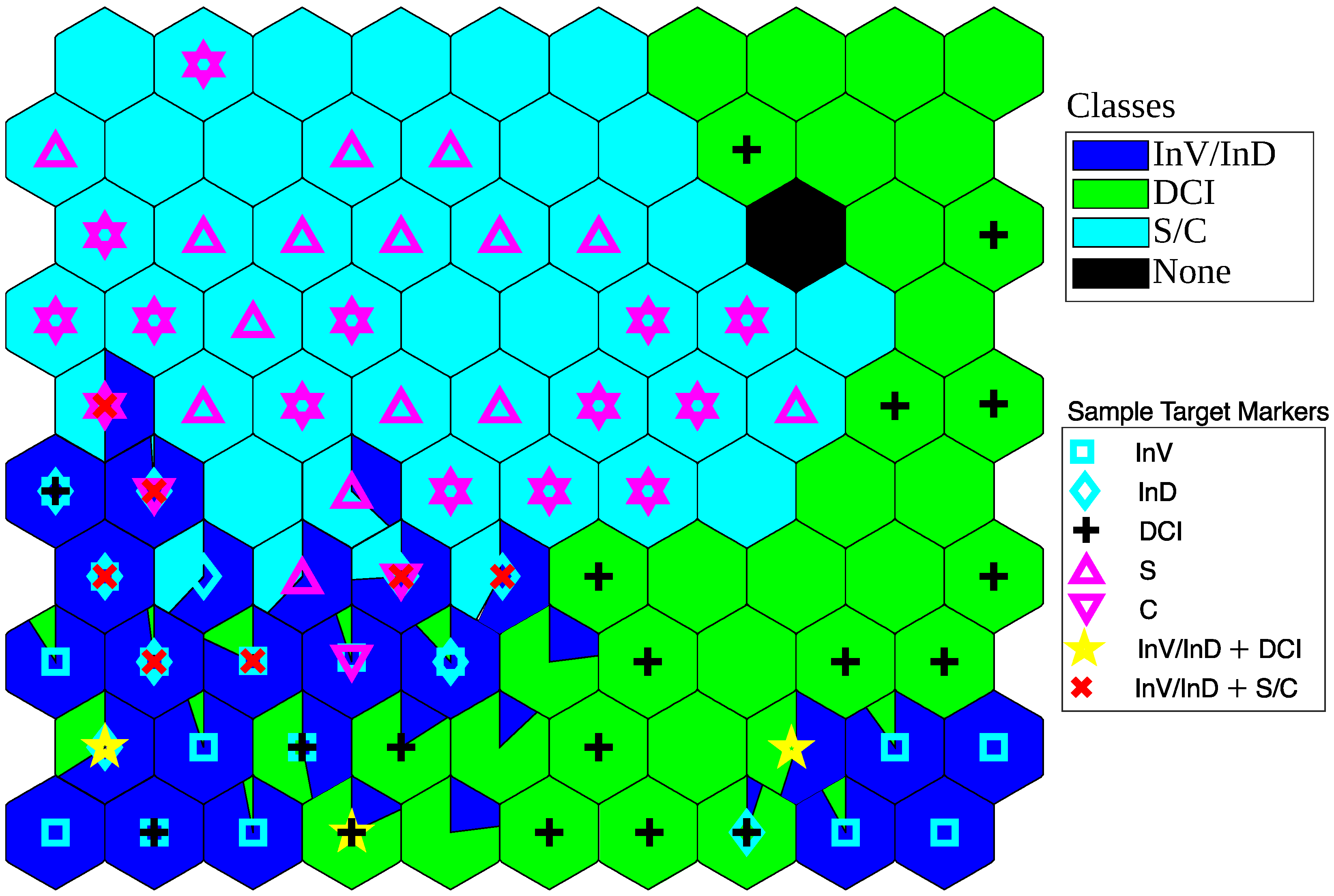
Furthermore, for a clearer illustration of how SOPM operates, the labels of the samples that excited the neurons were plotted on the probability map, as shown in Figure 16. It can be seen in Figure 16 that most of the samples were classified according to their respective classes, for single- or multi-class-featured cases.

Table 4. SOPM confusion matrix obtained using training samples, where bold values highlight correct classification rates.

True Class	Predicted Class
	Inv/InD	DCI	S/C
Inv/InD	97.00%	2.93%	0.07%
DCI	2.60%	97.40%	0.00%
S/C	0.00%	0.00%	100%

shows the obtained confusion matrix for training stage. The obtained accuracy varies from 97% to 100%. The observed high levels of accuracy are expected for the training procedures. Furthermore, for the threshold optimization stage, in which $r_1$ and $r_2$ are optimized for maximizing classification accuracy on the so-called optimization subset of samples, accuracy ranges from 93.50% to 100%, as seen in

Table 5. SOPM confusion matrix obtained using optimization samples, where bold values highlight correct classification rates.

True Class	Predicted Class
	Inv/InD	DCI	S/C
Inv/InD	93.50%	4.11%	2.39%
DCI	2.17%	97.83%	0.00%
S/C	0.00%	0.00%	100%

, which shows the success of the optimization process.

Finally,

Table 6. SOPM confusion matrix obtained using test samples, where bold values highlight correct classification rates.

True Class	Predicted Class
	Inv/InD	DCI	S/C	Inv/InD + DCI	Inv/InD + S/C
Inv/InD	86.75%	8.88%	4.37%	0.00%	0.00%
DCI	24.23%	75.77%	0.00%	0.00%	0.00%
S/C	6.84%	0.00%	91.37%	1.79%	0.00%
Inv/InD + DCI	0.00%	0.00%	0.00%	100%	0.00%
Inv/InD + S/C	0.00%	3.44%	9.69%	0.00%	86.87%

shows the confusion matrix obtained for test samples by using our SOPM method. Test samples are PRPDs not used on previous stages. It can be seen that SOPM has good performance, presenting accuracy rates from 75.77% for DCI class (minimum obtained accuracy rate) to 100% for InV/InD+DCI, which is a multiple-class featured group. The obtained results indicates that the developed method is working as expected when classifying single- or multiple-class samples. Note that when test samples are used, an average accuracy rate of $88.21\%$ was achieved, which is comparable to what is seen in the literature for single-class sample classifiers [8,9,10,11,12].

7.3. Discussion on Features of Samples Mapped on SOPM

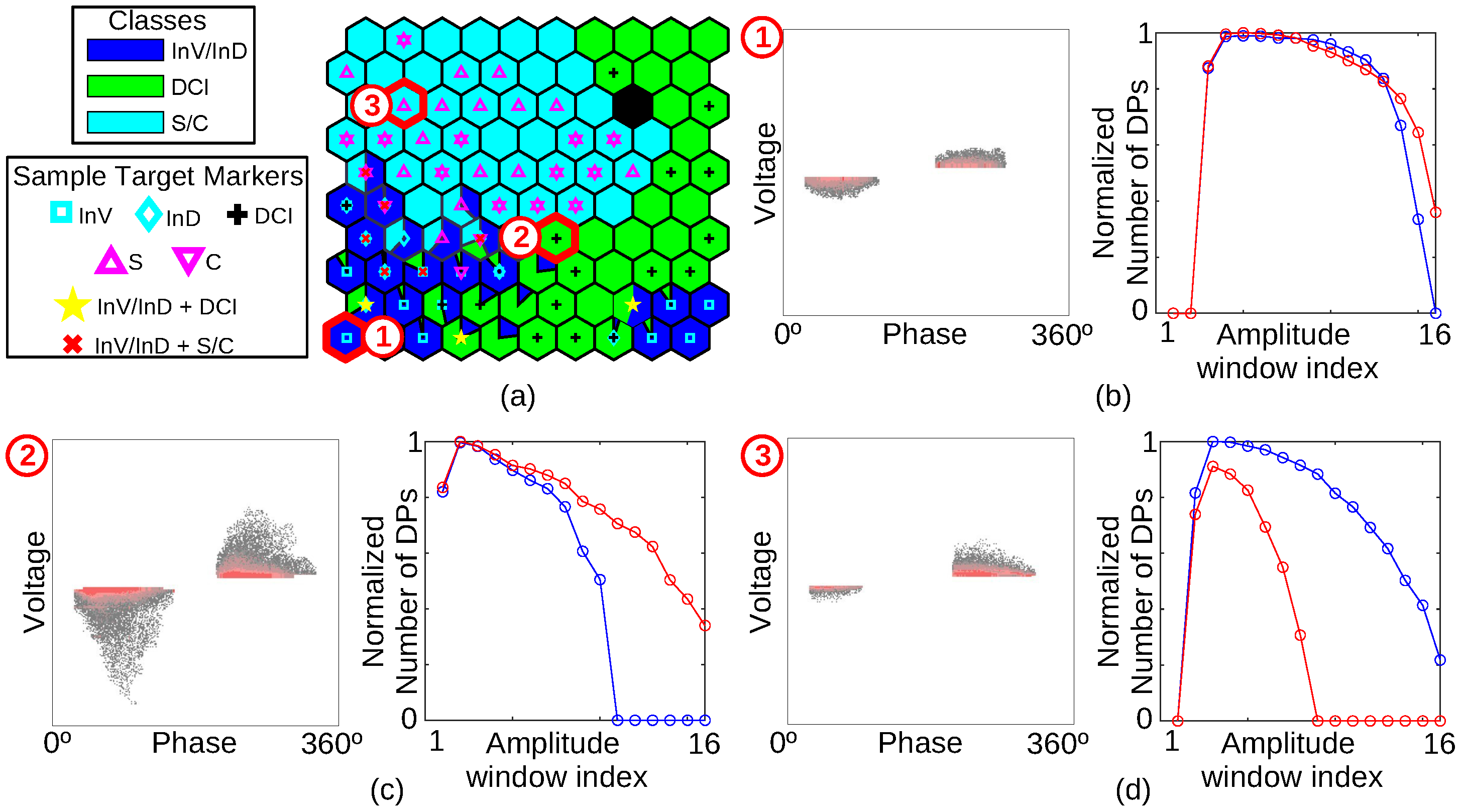
In this Section, we provide a detailed examination of PRPDs and their respective histograms for selected samples on our SOPM map. Figure 17a illustrates the SOPM map with three highlighted and numbered neurons of interest, each one associated with a distinctly specific class: InV/InD (neuron 1), DCI (neuron 2) and S/C (neuron 3). The neurons of interest were chosen because of their single-class associations and due to their positioning relative to class transition zones. Figure 17b–d show the PRPDs and histograms of samples activating the neurons of interest (neurons 1, 2, and 3, respectively).

In PRPDs graphs, reddish colors represent high PD count levels, while grayish tones are associated with low PD repetition rates. On the other hand, the blue lines in histograms’ plots represent normalized PD counts of PRPD clouds with positive voltage levels, whereas red lines are associated with normalized PD counts of PRPD clouds with negative voltage levels. Positive-voltage and negative-voltage PD count histograms have been obtained using sixteen voltage windows each [8].

In Figure 17b, the PRPD and PD-count amplitude histograms of the InV/InD-class sample are depicted. Notably, the PD-count amplitude histograms reveal comparable PD counts for positive- and negative-voltage clouds over amplitude windows, i.e., there is symmetry between the positive and negative clouds. This is a characteristic trait of the InV/InD class. Conversely, for the DCI sample, its histograms portray higher PD-count values for the negative-voltage cloud, as seen in Figure 17c, which is a characteristic attribute of the DCI class. Finally, regarding the S/C sample, Figure 17d showcases positive asymmetry, i.e., its histograms show higher PD-count values for the positive-voltage cloud, which is the main property characterizing the S/C class.

In contrast to single-class samples, multi-class samples lack a distinct symmetry or asymmetry between positive- and negative-voltage clouds in amplitude histograms. In order to better illustrate this aspect, two neurons, A and B, situated in class transition zones of SOPM, separating regions associated with InV/InD and S/C classes and regions linked to InV/InD and DCI classes, were chosen for visualizing and analyzing multi-class samples PRPD and histograms, as shown by Figure 18. Figure 18b illustrates PRPD and amplitude histograms of a multi-class sample with simultaneous features of the classes InV/InD and S/C, which excited transition neuron A. It is notable that the positive- and negative-voltage histograms exhibit close values (specially for amplitude window indexes under 11), a feature associated with the class InV/InD. However, the negative-voltage histogram displays a slightly steeper decline as amplitude window index increases, reaching zero at the index numbered as 13. This tendency suggests a potential classification of the sample as S/C, as previously discussed. Upon closer examination, when comparing the sample depicted in Figure 18b with those presented in Figure 17b,d, it becomes evident that the sample under analysis occupies a middle ground between the two mentioned classes, which shows proper classification of the sample by SOPM, as one can see in class probabilities distribution of neuron A in Figure 18a, which indicates a classification probability slightly higher for the class InV/InD than for the class S/C.

Finally, Figure 18c illustrates the PRPD and amplitude histograms for a multi-class sample, exciting neuron B, with simultaneous features of the classes InV/InD and DCI. Notably, while both positive- and negative-voltage histograms display comparable values across the amplitude window index, particularly for indexes under 12, indicating a possible classification as InV/InD, the positive-voltage histogram demonstrates a more pronounced decline than its negative-voltage counterpart. Despite this subtle asymmetry, upon comparing Figure 18c with Figure 17c, it becomes apparent that the sample also has DCI features, since the positive-voltage histogram exhibits a sharper decay, eventually reaching zero at the amplitude index 16 for the multi-class sample, which is not seen for the negative-voltage histogram. Consequently, this sample exhibits characteristics indicative of both of the classes InV/InD and DCI. As one can see in neuron B of Figure 18a, this is what SOPM is indicating, with a modestly superior probability in favor of InV/InD.

8. Conclusions

In this study, we proposed a self-organized probability map (SOPM) method for detecting and classifying partial discharges (PDs) in hydro-generators. The system was tested with samples obtained from online hydro-generator, and the results shows that it is capable of accurately classifying PRPDs with simultaneous features of several classes with classification accuracy comparable to previously published classifications methods designed to perform single-class sample classification (around 90% with test samples).

As the energy landscape evolves towards increased reliance on renewable sources and distributed generation, ensuring the reliability and longevity of critical power infrastructure becomes increasingly important. The SOPM method proposed in this work contributes to this goal by offering a robust and efficient tool for PD diagnostics in hydro-generators, key components of many renewable energy systems. By enabling accurate classification of complex, multi-class PD patterns, the SOPM method facilitates early detection of insulation degradation, allowing for timely maintenance interventions and preventing catastrophic failures. This not only enhances the reliability of hydro-power generation but also contributes to the overall stability and sustainability of the power grid. Moreover, the SOPM method’s potential applicability to other diagnostic and classification problems apart from PDs suggests broader implications for the future of energy, including applications in the monitoring and maintenance of wind turbines, solar panels and other renewable energy technologies. As the energy sector embraces digitalization and data-driven approaches, the SOPM method represents a pioneering step towards intelligent and automated fault diagnosis, paving the way for more stable energy systems in the future.

In contrast to previously published PD classification methods, which primarily focus on single-class PD patterns and achieve accuracy rates around 90%, the proposed SOPM method demonstrates the capability to accurately classify PRPDs containing simultaneous features of multiple PD classes. This advantage stems from the unique combination of a Kohonen network with statistical analysis, allowing the SOPM to map input data into a two-dimensional space and assign classification probabilities to each neuron. By incorporating a feature space with average distances between each neuron to n samples nearest to it, regarding each class, the SOPM gains a deeper understanding of the complex relationships between different PD classes and their manifestations in PRPDs. This, in turn, enables the SOPM to effectively disentangle overlapping features and provide reliable classifications even when dealing with the real-world complexities of multiple concurrent PD phenomena. As a result, the SOPM offers a more comprehensive and robust diagnostic tool compared to traditional methods, particularly in scenarios where multiple PD sources are present. Further research is suggested to evaluate the SOPM method’s applicability to other types of classification problems, not only related to partial discharges, potentially extending its benefits beyond the realm of PD diagnostics to many other areas of science.

References

1. IEC TS 60034-27:2006; Rotating Electrical Machines—Part 27-2: On-Line Partial Discharge Measurements On The Stator Winding Insulation Of Rotating Electrical Machines. IEC: Geneva, Switzerland, 2006.
2. Stone, G.C.; Culbert, I.; Boulter, E.A.; Dhirani, H. Electrical Insulation for Rotating Machines, 2nd ed.; IEEE Press Series on Power Engineering; Wiley-Blackwell: Hoboken, NJ, USA, 2012. [Google Scholar]
3. Stone, G.C.; Cavallini, A.; Behrmann, G.; Serafino, C.A. Practical Partial Discharge Measurement on Electrical Equipment; Wiley-IEEE Press: New York, NY, USA, 2023. [Google Scholar]
4. Cruz, J.S.; Fruett, F.; Lopes, R.R.; Takaki, F.L.; Tambascia, C.A.; Lima, E.R.; Giesbrecht, M. Partial Discharges Monitoring for Electric Machines Diagnosis: A Review. Energies 2022, 15, 7966. [Google Scholar] [CrossRef]
5. Machado, G.d.O.; Gomes, L.C.; da Silveira, A.W.F.V.; Tavares, C.E.; de Andrade, D.A. Impacts of Harmonic Voltage Distortions on the Dynamic Behavior and the PRPD Patterns of Partial Discharges in an Air Cavity Inside a Solid Dielectric Material. Energies 2022, 15, 2650. [Google Scholar] [CrossRef]
6. Lalitha, E.; Satish, L. Wavelet analysis for classification of multi-source PD patterns. IEEE Trans. Dielectr. Electr. Insul. 2000, 7, 40–47. [Google Scholar] [CrossRef]
7. Krivda, A.; Gulski, E. Neural networks as a tool for recognition of partial discharges. In Proceedings of the 1993 International Conference on Partial Discharge, Canterbury, UK, 28–30 September 1993; pp. 84–85. [Google Scholar]
8. Araújo, R.C.F.; de Oliveira, R.M.S.; Brasil, F.S.; Barros, F.J.B. Novel Features and PRPD Image Denoising Method for Improved Single-Source Partial Discharges Classification in On-Line Hydro-Generators. Energies 2021, 14, 3267. [Google Scholar] [CrossRef]
9. Lopes, F.H.; Zampolo, R.F.; Oliveira, R.M.; Dmitriev, V. Evaluation of transfer learning approaches for partial discharge classification in hydrogenerators. In Proceedings of the 2022 Workshop on Communication Networks and Power Systems (WCNPS), Fortaleza, Brazil, 17–18 November 2022; pp. 1–6. [Google Scholar]
10. Pardauil, A.C.N.; Nascimento, T.P.; Siqueira, M.R.S.; Bezerra, U.H.; Oliveira, W.D. Combined Approach Using Clustering-Random Forest to Evaluate Partial Discharge Patterns in Hydro Generators. Energies 2020, 13, 5992. [Google Scholar] [CrossRef]
11. Zemouri, R.; Lévesque, M.; Kokoko, O.; Hudon, C. Generative Adversarial Networks used for latent space Optimization: A comparative study for the Classification of Partial Discharge Sources. In Proceedings of the PHM Society European Conference, Prague, Czech Republic, 3–5 July 2021; Volume 6, p. 10. [Google Scholar]
12. Zemouri, R.; Lévesque, M. Ensemble Deep-Learning Model for Phase-Resolved Partial Discharge Diagnosis in Hydrogenerators. IEEE Trans. Dielectr. Electr. Insul. 2023, 30, 2394–2401. [Google Scholar] [CrossRef]
13. Dang, N.Q.; Ho, T.T.; Vo-Nguyen, T.D.; Youn, Y.W.; Choi, H.S.; Kim, Y.H. Supervised Contrastive Learning for Fault Diagnosis Based on Phase-Resolved Partial Discharge in Gas-Insulated Switchgear. Energies 2024, 17, 4. [Google Scholar] [CrossRef]
14. Florkowski, M. Classification of Partial Discharge Images Using Deep Convolutional Neural Networks. Energies 2020, 13, 5496. [Google Scholar] [CrossRef]
15. Basharan, V.; Siluvairaj, W.I.M.; Velayutham, M.R. Recognition of multiple partial discharge patterns by multi-class support vector machine using fractal image processing technique. IET Sci. Meas. Technol. 2018, 12, 1031–1038. [Google Scholar] [CrossRef]
16. Castro Heredia, L.C.; Rodrigo Mor, A. Density-based clustering methods for unsupervised separation of partial discharge sources. Int. J. Electr. Power Energy Syst. 2019, 107, 224–230. [Google Scholar] [CrossRef]
17. Hudon, C.; Belec, M. Partial discharge signal interpretation for generator diagnostics. IEEE Trans. Dielectr. Electr. Insul. 2005, 12, 297–319. [Google Scholar] [CrossRef]
18. Stone, G.C.; Warren, V. Objective methods to interpret partial-discharge data on rotating-machine stator windings. IEEE Trans. Ind. Appl. 2006, 42, 195–200. [Google Scholar] [CrossRef]
19. de Oliveira, R.M.S.; Araújo, R.C.F.; Barros, F.J.B.; Segundo, A.P.; Zampolo, R.F.; Fonseca, W.; Dmitriev, V.; Brasil, F.S. A system based on artificial neural networks for automatic classification of hydro-generator stator windings partial discharges. J. Microwaves Optoelectron. Electromagn. Appl. 2017, 16, 628–645. [Google Scholar] [CrossRef]
20. Stone, G.C. A perspective on online partial discharge monitoring for assessment of the condition of rotating machine stator winding insulation. IEEE Electr. Insul. Mag. 2012, 28, 8–13. [Google Scholar] [CrossRef]
21. Leffler, J.; Trnka, P. Failures of Electrical Machines-Review. In Proceedings of the 2022 8th International Youth Conference on Energy (IYCE), Eger, Hungary, 6–9 July 2022; pp. 1–4. [Google Scholar]
22. Raymond, W.J.K.; Illias, H.A.; Mokhlis, H. Partial discharge classifications: Review of recent progress. Measurement 2015, 68, 164–181. [Google Scholar] [CrossRef]
23. Luo, Y.; Li, Z.; Wang, H. A review of online partial discharge measurement of large generators. Energies 2017, 10, 1694. [Google Scholar] [CrossRef]
24. Araújo, R.C.F.; de Oliveira, R.M.S.; Barros, F.J.B. Automatic PRPD Image Recognition of Multiple Simultaneous Partial Discharge Sources in On-Line Hydro-Generator Stator Bars. Energies 2022, 15, 326. [Google Scholar] [CrossRef]
25. Stone, G.C. Partial discharge diagnostics and electrical equipment insulation condition assessment. IEEE Trans. Dielectr. Electr. Insul. 2005, 12, 891–904. [Google Scholar] [CrossRef]
26. Kohonen, T. Analysis of a simple self-organizing process. Biol. Cybern. 1982, 44, 135–140. [Google Scholar] [CrossRef]
27. Haykin, S.O. Neural Networks and Learning Machines, 3rd ed.; Pearson: Upper Saddle River, NJ, USA, 2008. [Google Scholar]
28. Vesanto, J. SOM-based data visualization methods. Intell. Data Anal. 1999, 3, 111–126. [Google Scholar] [CrossRef]
29. Kohonen, T. Self-Organizing Maps; Springer Science & Business Media: New York, NY, USA, 2012; Volume 30. [Google Scholar]
30. Kohonen, T. Essentials of the self-organizing map. Neural Netw. 2013, 37, 52–65. [Google Scholar] [CrossRef] [PubMed]
31. de Oliveira, V.Y.M.; de Oliveira, R.M.S.; Affonso, C.M. Cuckoo Search approach enhanced with genetic replacement of abandoned nests applied to optimal allocation of distributed generation units. IET Gener. Transm. Distrib. 2018, 12, 3353–3362. [Google Scholar] [CrossRef]
32. Han, Y.; Song, Y. Using improved self-organizing map for partial discharge diagnosis of large turbogenerators. IEEE Trans. Energy Convers. 2003, 18, 392–399. [Google Scholar] [CrossRef]
33. Darabad, V.; Vakilian, M.; Blackburn, T.; Phung, B. An efficient PD data mining method for power transformer defect models using SOM technique. Int. J. Electr. Power Energy Syst. 2015, 71, 373–382. [Google Scholar] [CrossRef]
Figure 1. Examples of PRPD maps in the data set. Each sample is associated with a PD class: (a) Slot Discharge (S), (b) Internal Void (InV), (c) Internal Delamination (InD), (d) Delamination Between Conductor and Insulation (DCI), (e) Corona (C), (f) Inv/InD + DCI and (g) Inv/InD + S/C.
Energies 17 02208 g001
Figure 2. PRPD map as seen (a) before filtering and (b) after filtering.
Energies 17 02208 g002
Figure 3. Quantity of PRPDs in each class of the data set.
Energies 17 02208 g003
Figure 4. Illustrations of (a) neurons, BMU and samples distributed in a didactic 2D space of features ( m = 2 ), (b) A 2D SOM network with input layer, output layer (the two-dimensional map itself), input sample, neural weights, and BMU and (c) SOM map with each neuron labeled as the class of its exciting samples (BMU is also highlighted).
Energies 17 02208 g004
Figure 5. Illustration of an update step of the best-matching unit and its neighbor neurons towards the input sample X in the didactic two-dimensional space of features.
Energies 17 02208 g005
Figure 6. Flowchart illustrating the employed SOM training algorithm. N is the total number of samples.
Energies 17 02208 g006
Figure 7. Calculation of D i k using n = 2 : (a) neurons and samples in the didactic space of features x 1 - x 2 , where the black lines defining d i , j k cross neuron w i and the two closer samples from each class k, (b) neuron w i and points to which distance D i k is calculated in the space of features for each class k and (c) distances D i k on a distance d-axis for k ranging between 1 and 3.
Energies 17 02208 g007
Figure 8. Representation of neuronal neighborhood regions in the didactic space of features regarding neuron w i with (a) samples and thresholds r 1 and r 2 and (b) distances D i k . (c) The neuronal neighborhood regions, distances D k i , and thresholds r 1 and r 2 in the distance space.
Energies 17 02208 g008
Figure 9. Cases in which P i 1 = 100 % because: (ac) exclusively D i 1 r 1 ; and (d) D i 2 > r 2 and D i 3 > r 2 with r 1 < D i 1 r 2 . Note that the neuron is represented by the blue color (associated with class 1). Classification probabilities are proportional to the areas covered by each color in the probability neural representation.
Energies 17 02208 g009
Figure 10. Examples in which w i is associated with more than one class. The related classes are (a,b) classes 1 and 3 because D i 1 r 1 and D i 3 r 1 ; and (c) classes 1, 2 and 3, since D i 1 r 1 , D i 2 r 1 and D i 3 r 1 . Note that the neuron is represented with the colors blue and cyan in (a,b), which are associated with classes 1 and 3, and by the colors blue, green, and cyan in (c), which are associated with classes 1, 2, and 3. Classification probabilities are proportional to the areas covered by each color in the probability neural representation.
Energies 17 02208 g010
Figure 11. Illustrative scenarios depicting the associations of w i with multiple classes or no class, in which it is (a) linked to classes 1 and 2 because r 1 < D i 1 r 2 , r 1 < D i 2 r 2 , and D i 3 > r 2 ; (b) associated with classes 1, 2, and 3, since r 1 < D i k r 2 for all k and (c) not linked to any class, as D i k > r 2 for all k.
Energies 17 02208 g011
Figure 12. An illustrative example of a self-organizing probability map (SOPM).
Energies 17 02208 g012
Figure 13. Flowchart with the algorithm developed for building and testing SOPM statistical classification.
Energies 17 02208 g013
Figure 14. The obtained 10 × 10 -SOM Map, with τ = 2000: (a) the Kohonen Map, in which regions with no clear separation among class clusters are observed, (b) SOM with white lines defining borders of class clusters, and (c) classes are assigned to each cluster according to labels of samples exciting neurons.
Energies 17 02208 g014
Figure 15. 10 × 10 -SOM-network with τ = 2000 and its (a) Kohonen map and (b) the probability map (SOPM) obtained using the proposed method.
Energies 17 02208 g015
Figure 16. SOPM with the exciting samples on their respective map neurons.
Energies 17 02208 g016
Figure 17. Single-class SOPM analysis of samples: (a) SOPM with highlighted and numbered single-class neurons associated with InV/InD (neuron 1), DCI (neuron 2), and S/C (neuron 3); and PRPDs and PD-count amplitude histograms of single-class samples identified as (b) InV/InD, (c) DCI, and (d) S/C. In histogram plots, the blue lines represent normalized PD counts of PRPD clouds with positive voltage levels and red lines are similarly associated with negative voltage levels.
Energies 17 02208 g017
Figure 18. Multi-class SOPM analysis of samples: (a) SOPM with two highlighted multi-class neurons associated with InV/InD+S/C and InV/InD+DCI; and PRPDs and amplitude histograms of multi-class samples classified as (b) InV/InD+S/C and (c) InV/InD+DCI. In histogram plots, the blue lines represent normalized PD counts of PRPD clouds with positive voltage levels and red lines are similarly associated with negative voltage levels.
Energies 17 02208 g018