Review

Energy Forecasting: A Comprehensive Review of Techniques and Technologies

by
Aristeidis Mystakidis
1,2,
Paraskevas Koukaras
1,2,
Nikolaos Tsalikidis
2,
Dimosthenis Ioannidis
2 and
Christos Tjortjis
1,*
1
School of Science and Technology, International Hellenic University, 14th km Thessaloniki-Moudania, 57001 Thessaloniki, Greece
2
Information Technologies Institute, Centre for Research & Technology, 57001 Thessaloniki, Greece
*
Author to whom correspondence should be addressed.
Energies 2024, 17(7), 1662; https://doi.org/10.3390/en17071662
Submission received: 4 March 2024 / Revised: 26 March 2024 / Accepted: 28 March 2024 / Published: 30 March 2024
(This article belongs to the Special Issue Artificial Intelligence in Energy Efficient Buildings)

Abstract

:
Distribution System Operators (DSOs) and Aggregators benefit from novel energy forecasting (EF) approaches. Improved forecasting accuracy may make it easier to deal with energy imbalances between generation and consumption. It also helps operations such as Demand Response Management (DRM) in Smart Grid (SG) architectures. For utilities, companies, and consumers to manage energy resources effectively and make educated decisions about energy generation and consumption, EF is essential. For many applications, such as Energy Load Forecasting (ELF), Energy Generation Forecasting (EGF), and grid stability, accurate EF is crucial. The state of the art in EF is examined in this literature review, emphasising cutting-edge forecasting techniques and technologies and their significance for the energy industry. It gives an overview of statistical, Machine Learning (ML)-based, and Deep Learning (DL)-based methods and their ensembles that form the basis of EF. Various time-series forecasting techniques are explored, including sequence-to-sequence, recursive, and direct forecasting. Furthermore, evaluation criteria are reported, namely, relative and absolute metrics such as Mean Absolute Error (MAE), Root Mean Square Error (RMSE), Mean Absolute Percentage Error (MAPE), Coefficient of Determination ( R 2 ), and Coefficient of Variation of the Root Mean Square Error (CVRMSE), as well as the Execution Time (ET), which are used to gauge prediction accuracy. Finally, an overall step-by-step standard methodology often utilised in EF problems is presented.

1. Introduction

The energy sector is undergoing significant changes on a worldwide scale, with a focus on energy efficiency, Smart Grid (SG) technologies, and a shift towards renewable energy sources. Precise and trustworthy EF is now essential in an ever-changing environment for ensuring efficient energy management, maintaining the supply and demand equilibrium, maximising resource use, and strengthening power system resilience [1].
The goal of Energy Forecasting (EF) is to predict future trends in energy generation, consumption, and distribution using a variety of approaches and procedures. These projections are essential for informing decision-makers in various fields, such as utilities, business, government, and Smart Cities (SCs) [2]. Proactive planning, efficient resource allocation, and grid integration of renewable energy sources are made possible by the capacity to predict patterns of energy generation and demand. Creating more effective Demand Response (DR) methods is the outcome of practical implications that lead to the cooperation of energy stakeholders, including Distribution System Operators (DSOs) and Aggregators.
This literature overview investigates the complex field of EF, examining the basic ideas, various algorithms, and cutting-edge tactics developed in recent studies. It examines the uses of statistical, Machine Learning (ML), and Deep Learning (DL) techniques in the context of EF. It also explores the effectiveness of ensemble approaches in improving prediction reliability and accuracy. In addition, a thorough analysis of time-series forecasting, the foundation of energy prediction, including direct, recursive, and sequence-to-sequence forecasting techniques, is provided. The intricacies of forecasting models’ comparative analysis can be better understood by investigating the evaluation measures used to judge their performance.
The influence that EF has on Energy Load Forecasting (ELF) and Energy Generation Forecasting (EGF) highlights the significance of this field [3]. This review investigates the following topics:
  • ELF for estimating energy demand in various settings, such as residential, commercial, etc. It analyses several methods in various operational conditions, time frames, and geographic areas. Such an assessment may assist stakeholders in making informed decisions on resource allocation, grid management, and energy efficiency by identifying the most effective forecasting methods for their particular situation.
  • EGF based on data from various renewable energy sources, such as solar and wind. The evaluation examines the effectiveness of forecasting methods for different set-ups, focusing on how they perform under various weather situations. Such an analysis is essential for determining the most effective ways to forecast power generation in various situations, offering useful insights for improving resource allocation and promoting sustainable energy management practices.
Therefore, both ELF and EGF play pivotal roles in maintaining grid stability, preventing overloads, and guaranteeing a smooth transition to a more sustainable energy ecology, all depending on the ability to understand and predict energy supply and demand.
In addition, numerous advantages can result from applying EF and subsequent Demand Response Management (DRM) techniques, as research has shown [4,5]. One benefit is a decline in energy use, which has favourable environmental effects, such as lower emissions. As noted in [6], there are also monetary advantages for building managers, end users, or tenants. EF is also essential for supporting efficient energy management and decision-making procedures. It gives SGs the necessary flexibility, enabling power distributors to efficiently coordinate and control future energy input and output. It helps energy suppliers to precisely forecast energy usage trends and be prepared for increased power demands [7], anticipating and responding to sudden demand spikes to ensure grid stability [8].
Thus, this review provides insights into the most recent developments and cutting-edge methods/approaches/tactics that support the field’s ongoing progress as it traverses the state of the art in EF. It provides the foundation for future research initiatives by identifying gaps, difficulties, and possibilities through a critical analysis of the existing literature.
The rest of this manuscript is structured as follows. Section 2 details the methodological tools utilised for this review work. Section 3 analyses various time horizons for load and generation forecasting while discussing the commonly utilised data parameters for performing EF. Section 4 examines the methods, models, and algorithms utilised for EF. These include statistical methods, ML/DL models, and ensemble methods. Section 5 explores time-series forecasting techniques and strategies, while Section 6 reports on the commonly used EF model evaluation metrics. Section 7 provides the standard methodological flow for performing EF. Section 8 discusses the findings, implications, and challenges of EF. Finally, Section 9 summarises the accomplishments/context of this work and also provides future directions on the topic of EF.

2. Materials and Methods

2.1. Primary and Secondary Data Source Collection

This study utilised primary data from targeted case studies on EF applications within DR frameworks in SGs. The studies were carefully chosen for their relevance to EF architectures and their potential to offer practical insights into EF deployment in energy systems. Complementing this, secondary data were collected through a thorough literature review, including peer-reviewed journals and industry reports. Together, these data sources provide a solid foundation for understanding EF technologies, their current implementations in energy systems, and their role in improving the efficiency of DR strategies.

2.2. Methodological Approach

This study adopted a qualitative framework. The thematic analysis focused on gaining insights into EF’s operational challenges and opportunities. This approach facilitated the identification of patterns and evaluated the effectiveness and limitations of EF architectures. The review process depicted in Figure 1 spanned over a hundred scholarly articles, focusing on EF’s integration into DR practices. The literature examination provided a theoretical foundation, enriching our analysis of empirical case studies, and was based on keywords and sources, as specified in Table 1. The selection criteria prioritised the relevance and contribution to EF’s knowledge base, as shown in Table 2. Consequently, theoretical and empirical findings were synthesised, elucidating EF’s impact on DR efficiency within SGs. This methodology underscores the intersection of practice and theory, offering a nuanced understanding of EF’s potential to optimise DR strategies.

2.3. Structured Research Progression

The research progressed through discrete yet interlinked phases:
  • Theoretical Foundation: Initial scrutiny of secondary data established the theoretical foundation and revealed research voids.
  • Case Study Analysis: The subsequent stage delved into case studies on EF within DR contexts in SGs, elucidating practical deployments.
  • Qualitative Analysis and Synthesis: An extensive qualitative assessment was conducted, interpreting EF’s practical implications for DR.
  • Conclusive Synthesis: The final phase integrated theoretical and empirical insights that informed comprehensive conclusions and outlined strategic avenues for future inquiry.

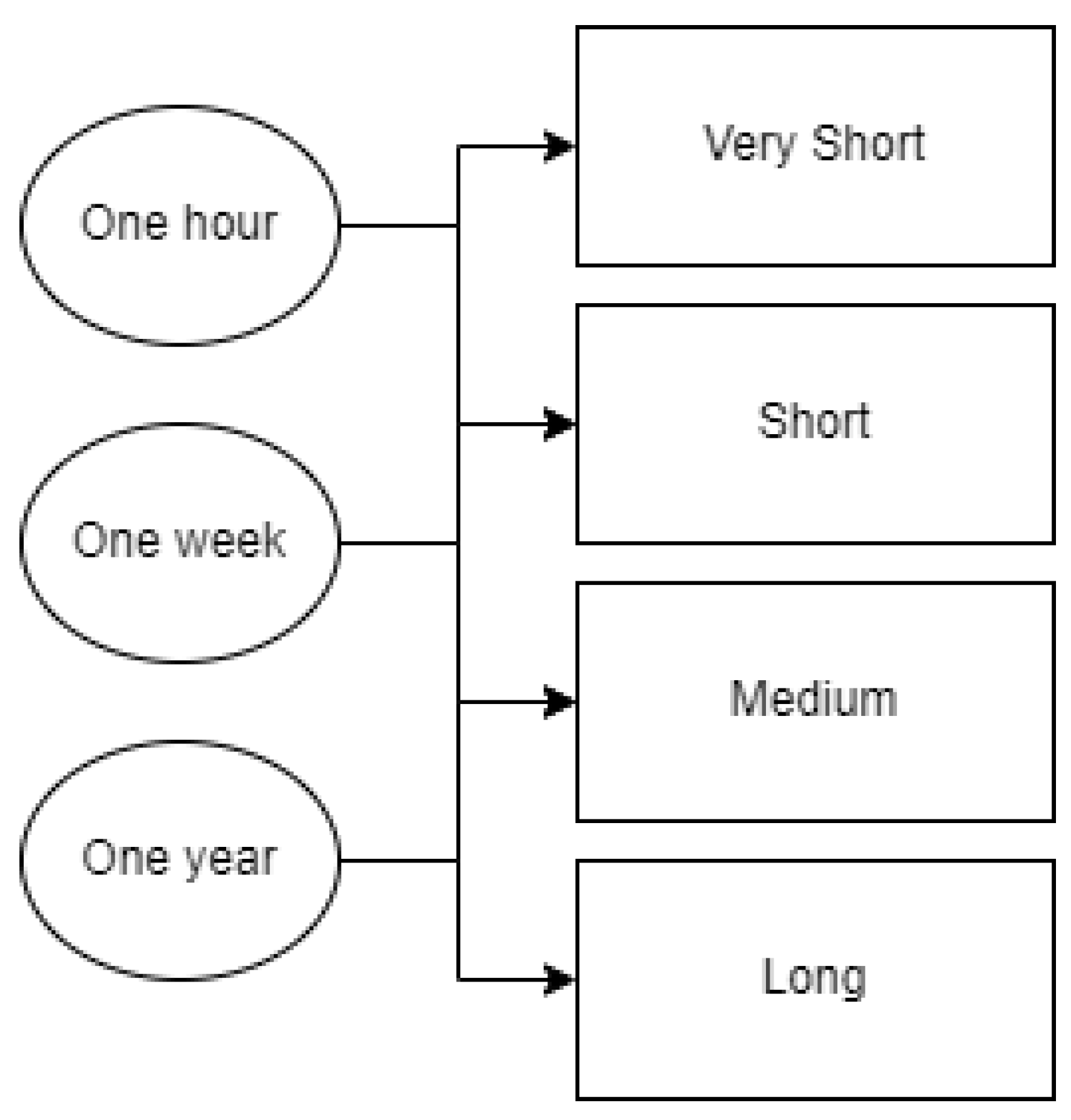
3. Energy Forecasting Horizons

In general, EGF and ELF were classified similarly with the same categorisation regarding their forecasting horizons [9,10]. According to [11,12], the field of ELF is divided into four primary forecasting horizon classes: Very Short-Term Load or Generation Forecasting (VSTLF or VSTGF), Short-Term Load or Generation Forecasting (STLF or STGF), Medium-Term Load or Generation Forecasting (MTLF or MTGF), and Long-Term Load or Generation Forecasting (LTLF or LTGF).
VSTLF and VSTGF, or Very Short-Term Forecasting (VSTF) for both, have projection ranges varying from a few minutes to an hour in advance, making it appropriate for ongoing surveillance. To predict load or generation from one hour to a day or a week in advance, STLF and STGF, or Short-Term Forecasting (STF) for both, are used [13]. With a focus on power system management and maintenance, MTLF and MTGF, or Medium-Term Forecasting (MTF) for both, forecast power consumption or generation for the upcoming weeks or months [14]. Finally, LTLF and LTGF, or Long-Term Forecasting (LTF) for both, are concerned with estimating the amount of electricity needed or generated in the next year or years [15]. The overall forecasting horizon classes are illustrated in Figure 2.
Depending on the forecasting horizon, different algorithms can be utilised, as discussed in Section 4). More specifically, statistical and linear models are more suitable for MTF and LTF, while TBMs perform better in STF and MTF. DL models can perform well regardless of the forecasting horizon.

3.1. Input Parameters for Load and Generation Forecasting

Three different types of inputs are commonly used with ELF. Examples of these include weather parameters like air temperature, relative humidity, precipitation, wind speed, and cloud cover; seasonal input variables like load variations due to air conditioning and heating (the month of the year, season, weekday, etc.); and historical load data (hourly loads for the hour prior, the day prior, and the day prior to the previous week). The daily peak load, weekly energy usage, and the projected load for each hour of the day are all output by ELF [16].
Similarly, the authors of [17] measured the most common input parameters utilised in more than 86 ELF research works, illustrating and categorising them into four categories. Weather and economic variables were used in 50% of them, household lifestyle in 8.33%, historical energy consumption/load in 38.33%, and stock indices in 3.33%.
Regarding EGF, the work of [18] proposed that time-varying parameters are very important for revealing nonlinear, fluctuating, and periodic patterns in time series in long-term Photovoltaic (PV) power generation forecasting. Moreover, the authors of [19] identified that PV power generation mainly depends on the amount of solar irradiance. In addition, other weather parameters, including atmospheric temperature, module temperature, wind speed and direction, and humidity, are considered as potential inputs.
In [20], the authors claimed that, among other factors, wind speed plays a vital role in the management, planning, and integration of wind EF systems. Other parameters include air temperature, air humidity, atmospheric pressure, average wind speed, and wind direction, as well as seasonal parameters and historical turbine velocity.
Meteorological data play a crucial role as input parameters for EGF and ELF. In addition to historical data, future weather data were utilised as inputs in works regarding EGF [21] and ELF [22]. These data were employed for the same time horizon as the specified step ahead of the target parameter (load or generation) that was being predicted.
The authors of [23] stated that Energy Planning Models (EPMs) played a critical role in identifying system boundaries and underlying relationships between the socio-technical parameters of energy, the economy, and the environment. This could include COVID-19 impacts, holidays, occupancy, or Key Performance Indicators (KPIs) like the reheat coefficient and building details’ measurements. Furthermore, the researchers of [24] also include indoor wireless sensors for temperature and humidity, among others.
Another important input to consider could be specific information about and characteristics of the facility or structure being targeted, especially when predicting the demand for huge facilities or residential buildings in certain industries. Therefore, Klyuev et al. [25] conducted experiments to provide managerial support in determining the optimal power consumption levels. To this end, a predictive model was developed to assess the potential power consumption of the power system. In addition, Chalal et al. [26] also considered factors such as users’ behaviour and buildings’ characteristics when developing forecasting models for the building industry.
A generic presentation of the input parameters regarding ELF or EGF is illustrated by category in Table 3.

3.2. Load Forecasting

At a building level, there are different types of energy loads, with the most common referring to heating, cooling, and electricity [3,27]. Besides these three, which are the most well-known, there are other types of energy referring to a non-building level, like thermochemical, pumped energy storage, magnetic, and chemical [28].
Moreover, at the building level, ELF finds applications in the optimal operation of both electric and thermal energy storage units, as well as the building’s Heating, Ventilation, and Air Conditioning (HVAC) system [29]. In the event that ELF and, consequently, DSM [4,5] result in a reduction in energy consumption, there are also environmental benefits (i.e., fewer emissions) and financial ones [6] for building managers or even for end-users or tenants.
Furthermore, another study suggests a sophisticated modular framework for STLF in SGs [30]. The researchers employed an altered version of a boosted differential evolution algorithm that utilises linear models in addition to Support Vector Machine (SVM) and Deep Neural Networks (DNNs). They suggest an approach that has been evaluated by experiments and validated on datasets for Ohio (DAYTOWN) and Kentucky (EKPC), USA, calculating performance via the Mean Absolute Percentage Error (MAPE), execution duration, and scalability. The findings demonstrated the improved results of the proposed model compared to two existing day-ahead load forecasting models.
Additionally, the authors of [29] used shallow ML and DL to predict a building’s thermal load. They employed twelve models, including vanilla DNNs, Linear Regression (LR), Extreme Gradient Boosting Regression (XGBR), Lasso Regression (LSR), Elastic Net (EN), SVM, Random Forest (RF), and Long Short-Term Memory (LSTM) Recurrent Neural Networks (RNNs). The findings indicate that the Coefficient of Variation of the Root Mean Squared Error (CVRMSE) scores range from 14.2% to 45%. More specifically, the data indicate that LSTM and XGBR are the most accurate shallow and DL models. As a result, they discovered that while LSTM performs poorly in long-term forecasts (24 h ahead), it performs better in short-term forecasts (1 h ahead). This is because sequential information loses significance and efficacy with vast forecasting scopes. Furthermore, the uncertainty associated with weather forecasting reduces the accuracy of XGBR and increases the robustness of LSTM due to the sequential knowledge.
Further, a Deep Belief Network (DBN)-based ensemble method was employed by the authors of [31] for air-conditioning cooling ELF. More precisely, they measured the Mean Absolute Error (MAE), Root Mean Square Error (RMSE), Coefficient of Determination ( R 2 ), MAPE, and CVRMSE metrics, which ranged from 12.72 to 25.48 kW, 9.44 to 16.04 kW, 2.4 to 4%, 21.4 to 27.9%, and 0.75 to 0.84, respectively, using a stacked Restricted Boltzmann Machine with a Logistic Regressor as the outcome.
Based on the Bagging-XGBR algorithm, the extreme weather identification and Short-Term Load Forecasting (STLF) model presented in [32] may offer an early warning on the time frame and specific value of peak demand. First, the XGBR algorithm-based Bagging concept is introduced, which aims to reduce the output variance and enhance the algorithm’s generalisation ability. Next, the Mutual Information (MI) between weather-affecting components and load is assessed to improve the model’s capacity to track weather variations. Then, considering the load, weather, and time factors, the extreme weather detection model is built to determine the peak load occurrence range. A high-accuracy STLF model is then created by choosing the specialised training set based on weighted similarity. The model presented in this study reduces the average MAPE of peak load by 3% to 10% when compared to the standard method.
Additionally, the researchers in [33] proposed a unique hybrid technique that combines Bi-directional Long Short-Term Memory (BiLSTM), Grey Wolf Optimisation (GWO), and Convolutional Neural Networks (CNNs) to predict building loads. GWO determines the optimal set of parameters for the CNN and BiLSTM algorithms. A one-dimensional CNN was utilised to effectively extract time-series data features. Using hourly resolution data, the performance of the proposed approach was investigated in four buildings with distinct features. The results confirm that the same approach may be successfully applied to various architectures.
The authors of [34] provide a data-driven predictive control technique that blends time-series forecasting and Reinforcement Learning (RL) to assess various sensor metadata to optimise HVAC systems. This involved designing and testing sixteen LSTM-based architectures with bi-directional, convolutional, and attention-processing mechanisms. The results show that recursive prediction greatly reduces model accuracy; this effect is more pronounced in the model for humidity and temperature prediction. In the surrogate environment, 17.4% energy savings and 16.9% improvement in thermal comfort are achieved by integrating the ideal TSF models with a Soft Actor–Critic RL agent to analyse sensor metadata and optimise HVAC operations.
Furthermore, another work addresses the problem of information loss owing to excessively long input time-series data by presenting a novel method for short-term power load forecasting that combines CNN, LSTM, and attention mechanisms [35]. Improving short-term power load prediction accuracy is the goal since it is essential to effective energy management. Using a Pearson correlation coefficient analysis, the study determined which elements have the most influence on the link between the goal load and the gathered values. After extracting high-dimensional features from the input data using a one-dimensional CNN layer, an LSTM layer is used to identify temporal correlations within historical sequences. An attention mechanism is finally included to maximise the weight of the LSTM output, strengthen the significance of important information, and improve the prediction model as a whole. Two benchmark algorithms based on MAPE, RMSE, and MAE metrics were used to assess the performance of the proposed model. According to the results, the CNN-LSTM-A model performs better than the conventional LSTM model regarding power load forecast accuracy for two thermal power units. There were improvements of 5.7% and 7.3%, respectively.

3.3. Generation Forecasting

The forecasting of PV energy has drawn a lot of interest. Numerous computational and statistical approaches are employed to enhance the precision of Electrical Energy Demand (EED) forecasts [36]. EGF models generally fall into two groups: direct and indirect forecasting models. The solar irradiation at the location where the PVs are positioned is predicted by indirect models. A range of techniques, such as hybrid Artificial Neural Networks (ANNs), statistical analysis, images, and Numerical Weather Prediction (NWP), were used to forecast the generation of PVs on various time scales [37]. The PV energy output and related meteorological data are used as historical data samples to forecast PV energy generation in direct forecasting models. To anticipate the energy generation of a PV system, another research used both direct and indirect approaches, and they concluded that the direct method was better [38].
A comparison of several scholarly articles on Energy Efficiency Directive (EEDi) predictions based on time frame, inputs, outcomes, application scale, and value was conducted by the researchers in [11]. The results of this investigation showed that, in contrast to AI-based models like ANNs, fuzzy logic, and SVM, which are suitable for STGF, regression models are primarily beneficial for LTGF, regardless of their simplicity.
Accurate STGF is complex to achieve. Forecasting solar radiation and PV power is a nonlinear problem that relies on several meteorological factors. It is very challenging to choose the best parameter estimation technique for a nonlinear situation. Numerous approaches to forecasting have been put forward in the literature; nevertheless, the choice of forecasting model is contingent upon the location and forecasting horizon. Effective information is extracted from the input training data by data-driven models, which then use this information to predict the output. The calibre of the training data affects how well these strategies function. The availability of such historical PV power data is a necessary prerequisite for direct PV forecasting, as ML techniques require some historical data for model training [21].
The two most often utilised ML methods in the field of PV forecasting are the ANN and SVM [39,40,41]. There are numerous ANN-related studies that support that Neural Networks’ (NNs) nonlinear fitting capability is superior to that of time-series models. The NN performance is a result of much research, ranging from an early simple architecture to a late deep configuration.
For ML algorithms, choosing the right hyperparameter values is crucial and significantly affects forecasting accuracy. For instance, two crucial SVM parameters, C and gamma, can have incorrect values that lead to overfitting and underfitting problems [42]. Consequently, many academics use intelligent optimisers to tune the hyperparameters of ML algorithms. By using an enhanced ACO to optimise SVM parameters, the research of [43] reported an improvement in the R 2 score from 0.991 to 0.997. Similar to this, the authors of [44] used a genetic algorithm, and [45] used enhanced swarm optimisation to adjust the Extreme Learning Machine’s (ELM) hyperparameters. Both studies reported increased forecast accuracy after incorporating optimisation algorithms. Furthermore, DL-based algorithms for PV power forecasting were given by [46,47], where the hyperparameters were optimised using Particle Swarm Optimisation (PSO) and Randomly Occurring Distributedly Delayed PSO (RODDPSO) approaches, respectively.
For PV power forecasting, the researchers in [48] employed a Bi-LSTM DL model. Following a comparison between the outcomes of different NN architectures and time-series modelling algorithms (ARMA, ARIMA, and SARIMA), it was shown that NNs had a greater predictive power while requiring fewer resources for computation. In contrast to traditional RNNs, LSTM networks have a memory unit that helps store long-term data and can also address the gradient descent problem. As a result, temporal information can be extracted from time-series data by LSTM. Comparably, in [49], a DBN was introduced to extract the nonlinear features from historical PV power time-series data. Additionally, a thorough review of optimisation-based hybrid models built on ANN models was given by the authors of [50].
A concept that establishes the best way to implement an irradiance-to-power conversion process using a mix of ML and physical techniques was studied [51]. Furthermore, a head-to-head comparison of physical, data-driven, and hybrid methodologies was carried out for the operational day-ahead power forecasting of 14 PV facilities in a pilot based on NWP. The authors devised two directives—reducing MAE and decreasing the RMSE—with different sets of predictions tailored for each directive to meet the consistency condition and get the widest overview feasible.
Records from a PV infrastructure in Cocoa, Florida, were employed by researchers [52]. The ANN approach outperformed the other algorithms in forecasting performance evaluations, yielding the best MAE, RMSE, and R 2 metrics of 0.4693, 0.8816 W, and 0.9988, respectively. The most dependable and appropriate algorithm for predicting PV solar power generation was proven to be the ANN.
Wang et al. [29] constructed 12 data-driven algorithms for shallow ML and DL. The results show that XGBR and LSTM are the most effective shallow and DL models, respectively. They determined that LSTM operates well for short-term prediction (1 h ahead) but not for long-term prediction (24 h ahead) since sequential information becomes less meaningful and valuable as the prediction horizon grows longer. Furthermore, including weather forecast inconsistency reduces XGBR accuracy and favours LSTM, as sequential information makes the algorithm more resilient to input error.
To solve shortcomings, the research of [53] suggests a hybrid framework for the power generation projection of diverse renewable energy sources. An attention-based LSTM (A-LSTM) network was designed to identify the nonlinear time-series features of weather and individual energy, a CNN was trained for obtaining local correlations among numerous energy sources, and an autoregression model was utilised to extract the linear time-series characteristics of each energy source. The suggested method’s correctness and applicability were confirmed using a renewable energy system. The outcomes demonstrate that the hybrid framework outperforms other sophisticated models, like decision trees (DTs) and ANNs, regarding accuracy. The proposed method’s MAEs decreased by 13.4%, 22.9%, and 27.1% for solar PV, solar thermal, and wind power, respectively, compared with those of A-LSTM.
Gaussian Processes (GPs) are one of the most interesting strategies for producing probabilistic forecasts. This study introduces and compares the Log-normal Process (LP) to the traditional GP. The LP was developed for positive data, such as home load forecasts, as this issue was previously overlooked [54].

4. Forecasting Methods/Models/Algorithms

This section reports statistical approaches, ML/DL methods/models/algorithms, and ensemble methods investigated in the literature following the analysis described in Section 2. An overview of these algorithms, along with the energy forecasting horizons (discussed in Section 3), is presented in Figure 3.

4.1. Statistical Methods

Statistical methods have long been the cornerstone of EF. They offer tools to model and predict energy consumption and production patterns. These methods leverage historical data to identify trends, seasonality, and other relevant patterns in energy systems. Table 4 summarises key statistical approaches, their applications in EF, and significant findings, providing an overview of their contributions to the field.
Most of the time, MTF focuses on Monthly Energy Forecasting (MEF). Random disturbances, annual seasonality, and nonlinear trends are all present in the MEF time series. They demonstrate a notable change in the annual cycle’s variance and structure with time. Climate and meteorological elements, in addition to socioeconomic and economic factors, have a significant impact on MEF. Unpredictable weather patterns, political actions, and economic events are some variables causing disruptions to the MEF [55]. The significance of MEF forecasting for the power industry and the intricacy of the issue motivate the quest for forecasting models that can produce precise forecasts while satisfying the task’s special needs.
MTF for power demand is a thoroughly studied topic. Numerous approaches have been taken to resolve this problem, including similarity-based approaches [56,57,58] and classical/statistical methods [59,60]. Initially, conventional methods were used to forecast the amount of electricity consumed. The exponential smoothing (ETS), ARIMA, and LR techniques have been applied extensively for over three decades [61].
Besides MTF, LTF is also frequently employed using linear and statistical models. For instance, the performance of the ARIMA and LR models in predicting monthly peak loads up to 12 months ahead of time was compared in [61,62]. The same set of inputs, which include historical peak demand data, meteorological data, and economic data, powered the algorithms. Test outcomes showed that the accuracy of the ARIMA model was around two times as high as that of the others.
To determine a relationship between energy usage and the influencing elements, statistical regression models rely upon previous performance information. This suggests that to train the models, enough historical data must be collected. Using basic variables, the method first predicts energy consumption and computes energy usage metrics, such as the gain factor, total heat capacity, and total heat loss coefficient, which are essential for analysing the thermal behaviour of buildings [63,64].
In simplified models, regression is occasionally used to establish an energy footprint to ascertain the relationship between energy use and climate variables [65]. Measurements collected for one day, one week, and three months were utilised to develop the regression model employed in the study by [66]. As a result, the annual energy consumption was predicted with prediction errors of 100%, 30%, and 6%, respectively. These results show that the length of the data period has a substantial effect on temperature-dependent regression models. The Auto-Regressive model with eXtra inputs (ARX) was utilised to estimate the U and g values of building components [67]. Although statistical methods are easily created, their accuracy and lack of flexibility are widely known limitations.
A description of the MTLF spatial autoregression model can be found in [68]. In the thirty Chinese provinces under analysis, the authors found a substantial link between GDP and system stress. In addition to using the local load dependence on GDP, they also used the relationships found for surrounding provinces to forecast the load in a specific province. This made it possible to lower forecast errors from 5.2–2.4% to 3.5–2.9%. The integration of bootstrap aggregation with ARIMA and ETS prognostic algorithms was presented in [62]. The Box–Cox transform, which is frequently used to account for variations, was first applied to the time series, and they were then decomposed. For the purpose of creating bootstrap tests, the ARMA model was utilised, while the ARIMA and ETS models were employed for forecasting.
Fourier series are also used in classical approaches. They were applied to the modelling of the seasonal part of the monthly load time series in [69]. Several key frequencies were found via spectral analysis, and the corresponding Fourier series were generated. The trend forecast was supplemented by the seasonal aspect of the forecast, which was computed using the Fourier series. In [70], Markov chains were exploited to evaluate the incoming data and determine which forecasting algorithm was most accurate. This method works particularly well when the time series’ upward tendency is erratic. The model shown in [71], which is predicated on a straightforward logistic function, is another example of a traditional model. Time, max air temperature, and holiday dates are the input variables.
Table 4. Summary of statistical methods for EF.
ReferencesModel/MethodApplicationsFindings
 [55]MEF Disruptions AnalysisMEFHighlighted the significant impact of climate, socioeconomic, and economic factors on MEF.
 [56,58]Similarity-based approachesMedium-Term ForecastingExplored similarity-based and classical methods for power demand forecasting.
 [61]ARIMA, LRMonthly peak load forecastingDemonstrated ARIMA’s higher accuracy in predicting monthly peak loads compared to LR.
 [62]Bootstrap aggregation with ARIMA and ETSForecasting with bootstrap testsEmployed bootstrap aggregation to enhance forecasting accuracy of ARIMA and ETS models.
 [63,64]Regression models for energy usage metricsThermal behaviour analysis of buildingsPredicted energy consumption and computed essential metrics for analysing building thermal behaviour.
 [65]Regression model for energy footprintEnergy use and climate variable relationshipEstablished a relationship between energy use and climate variables with varying prediction accuracy based on the data period length.
 [72]ARX modelEstimation of building components’ valuesUtilised the ARX model to estimate the U and g values of building components, highlighting the limitations of statistical methods in flexibility.
 [67]Spatial autoregression modelMid-/Long-Term Load ForecastingAnalysed the link between GDP and system stress for forecasting load with reduced errors.
 [68]Fourier series for seasonal modellingMonthly load time seriesApplied Fourier series to model the seasonal parts of monthly load time series, enhancing trend forecast.
 [69]Markov chains for an unstable growth sequenceMid-/Long-Term Load ForecastingEmployed Markov chains to address erratic upward trends in time-series forecasting.
 [70]Logistic Function ModelPeak demand forecastingUtilised a straightforward logistic model for long-range peak demand forecasting under high growth conditions.

4.2. Machine Learning Regression Models

In the context of ML, regression models are highly effective instruments used to forecast numerical results. This section examines different types of regression models, discussing their applications and important factors to consider.

4.2.1. Linear Models

LR can be considered both an ML and a statistical model, being a well-researched and the most basic algorithm for regression. While Multiple Linear Regression (MLR) is employed when several variables exist, typically referred to as a matrix of features, simple LR is utilised when a single input variable is provided. The weighted sum of the input characteristics is added to the bias term, often referred to as the intercept term, in an LR model to make predictions. If the LR model accurately depicts the facts, then no more complexity is needed. The effectiveness of LR is frequently verified using a cost function. The aim is to reduce the gap between the training observations and the linear model’s forecasts.
An extended LR model with periodic components implemented by using the sine function of different frequencies for non-stationary time series having an irregular periodic trend was suggested [73]. Also, there is an example of how to apply the LR model for medium- and long-term electrical load forecasting (MTLF and LTLF) [74]. The model forecasts daily load profiles in time horizons ranging from several weeks to many years using high correlations between daily (24 h) and yearly (52 weeks). Annual load increases are factored into the forecast estimates. The MAPE errors were found to have values no higher than 3.8% for forecasting within a one-year time frame.
A regularised form of LR called Ridge Regression (RR) was developed. One useful strategy to mitigate the issue of overfitting is to regularise the LR model. This is accomplished by limiting the model’s degree of freedom and decreasing the number of polynomial degrees, which makes overfitting more difficult. The least absolute shrinkage and selection operator regression, or Lasso, is another regularised version of LR. It augments the cost function with a regularisation component, just like RR [75].
Depending on the implementation (e.g., with a linear kernel), Support Vector Regression (SVR) is predicated on a high-dimensional feature space that is produced by altering the original variables and adding a term to the error function to penalise the complexity that results [76]. Because the cost function used to construct the model rejects any training data that are substantially close to the model prediction, the SVR-produced model only depends on a portion of the training data [77].
Other models include Elastic Net Regression (ENR) [78] and Lasso Least Angle Regression [79]. Furthermore, depending on how they are implemented and the context in which they are used, this category can include models like Polynomial Regression (PR) [80] and Bayesian Ridge Regression (BRR) [81]. The models presented in this review are given in Table 5.
Table 5. Summary of ML linear models for EF.
ReferencesModel/MethodApplicationsFindings
 [73]LR with periodic componentsNon-stationary time seriesEnhanced forecasting for irregular periodic trends using sine functions.
 [74]LR for medium- and long-term forecastingElectrical load forecastingDemonstrated effective daily load profile forecasting with MAPE errors under 3.8%.
 [75]Lasso and Ridge RegressionRegularisation of LRAddressed overfitting by adding regularisation components to the cost function.
 [76]SVRHigh-dimensional feature spaceUtilised a complexity penalisation term to focus on a subset of training data for model building.
 [77]SVR for training data selectionModel predictionEmphasised model dependency on a portion of the training data for construction.
 [78]ENRVariable selection and regularisation in high-dimensional dataLARS-EN algorithm proposed for efficient Elastic Net regularisation path computation.
 [79]Lasso Least Angle RegressionPrincipled choice among a range of possible estimates through a simple approximation and reduced computing timeEfficient model selection and regularisation in data modelling tasks/EF.
 [81]BRRData modelling tasksPresented methods for optimising regularisation constants and model comparison using evidence, enhancing model selection and complexity management.

4.2.2. Tree-Based Models

In general, tree-based models (TBMs) perform better than other models on data with zero values [82,83,84,85]. Since EF datasets can provide distributions with many zero values [21,22], TBMs can achieve better metric scores in both ELF and EGF. The ability of tree models to manage outliers gives them a significant advantage over linear models. When attributes do not exhibit a linear connection with the target variable, regression trees are expected to outperform linear models [86]. These are reliable algorithms that fit intricate datasets with success.
Considering that TBMs are a class of ML models that use DTs to classify or calculate the values of the target variable to carry out regression or classification tasks, it is important to mention that the basic TBM is the DT. As a supervised learning approach, the DT can be used for both regression and classification issues. A series of straightforward, binary decision rules are applied to perform data segmentation, as seen by the tree structure. These models develop criteria to forecast the numerical results of the variable being studied by splitting data repeatedly. Their main benefits are their easily understandable results and simple visualisation, in addition to the previously noted fact that they do not require data normalisation. They do not, however, generally outperform NN, particularly with regard to nonlinear data [87] for STF and MTF.
RF is another method that is utilised for both regression and classification. It is an ensemble method that uses the training data from several DTs to either classify or forecast a variable’s value. A certain number of features are randomly chosen for the split at each node of the DTs. Regression uses the mean or average value of the individual trees to determine the outcome, whereas the first scenario uses a majority vote on the results of the individual trees. RF is seen to be a fairly successful prediction tool because of the Law of Large Numbers, which prevents them from overfitting their training set, and the element of randomness [88].
A forest of extremely random trees is called the Extremely Randomised Trees ensemble or Extra-Trees. Just a random subset of the features are considered for splitting at each node while building a tree in a random field [89]. Unlike traditional DTs, which search for optimal thresholds, trees with even more random entries for every attribute can be created. By using this approach, a lower variance is traded for a bigger bias. Consequently, Extra-Trees train much quicker than traditional RFs. This is because determining the best threshold for each feature at each tree node takes very little time.
As an extension of TBMs, boosting models are ensemble methods that integrate and transform multiple weak learners into a more powerful learner [90]. Most boosting strategies revolve around the idea of training predictors one after the other in an attempt to fix the one that came before it. Gradient Boosting Regressor (GBR) [91] involves gradually adding predictors to an ensemble, each of which corrects the one before it. It achieves this without changing the instance weights throughout each iteration by fitting the new predictor to the residual errors produced by the prior predictor [90]. GBR has been used in studies that simulate the energy use of commercial buildings to anticipate the STF energy consumption of buildings [92]. GBR fared better than MLR and RF models when it came to predicting the energy usage of commercial buildings [93].
XGBR is a popular approach that uses scalable end-to-end tree boosting to produce state-of-the-art results on a range of ML problems involving both regression and classification. It is a novel weighted quantile sketch for approximation tree learning and a sparsity-aware technique for sparse data. Cache access patterns, data compression, and sharding were used in [94] to build a tree-boosting system that is thus scalable. By incorporating these findings, XGBR outperforms many algorithms in many scenarios while consuming significantly fewer resources.
There are many other popular boosting/TBMs utilised for EF. These include Light Gradient Boosting Machine Regressor (LGBMR) [95], Histogram-Based Gradient Boosting Regressor (HGBR) [91], Categorical Boosting Regressor (CBR) [96], AdaBoost Regressor (ABR) [97], and possibly others. A current overview is presented in Table 6.
Table 6. Summary of ML tree-based models for EF.
ReferencesModel/MethodApplicationsFindings
 [82,83,84,85]General TBMsELF and EGFHighlighted TBMs’ superior performance on datasets with many zero values and their ability to effectively manage outliers.
 [86]Regression treesPredicting household energy consumptionDemonstrated the advantage of TBMs in situations where attributes and target variables do not have linear connections.
 [87]DTsRegression and classificationShowed that DTs are easily interpretable but may not always outperform NNs, especially with nonlinear data.
 [88]RFRegression and classificationIndicated RF’s effectiveness as a prediction tool due to its ability to prevent overfitting through the Law of Large Numbers and randomness.
 [89]Extremely Randomised Trees (Extra-Trees)Supervised classification and regression problemsNoted for quick training times and trading lower variance for higher bias than traditional RFs.
 [90,91]GBREnergy use in commercial buildingsGBR outperformed MLR and RF models in predicting energy usage in commercial buildings.
 [94]XGBRVarious ML problemsAchieved state-of-the-art results with efficiency in resource usage.
 [91,95,96,97]Other boosting/TBMsEFIncluded various TBMs utilised for EF, showcasing the diversity and effectiveness of boosting methods.

4.3. Deep Learning Regression Models

DL regression models are powerful tools in EF, capable of capturing complex nonlinear relationships within large datasets. They range from CNNs for spatial data interpretation to RNNs for sequential data analysis and represent the cutting edge in predictive accuracy and model sophistication.
There are various EGF and ELF works implemented with DL and NNs [98,99] for VSTLF or VSTGF [21], STLF or STGF [22], MTLF or MTGF [100], and LTLF or LTGF [101].
The structure of interconnected nodes, or units known as artificial neurons, usually modelled after neurons in the biological brain, is known as an ANN. Like synapses in the neurological system, every link has the potential to communicate with neighbouring neurons. A neuron receives information, processes it, and can exchange messages with other neurons to which it is connected. The most basic neural network with input, hidden, and output layers is the Feedforward Neural Network (FNN), also called Multi-layer Perceptron (MLP) [102].
RNNs are a family of NNs intended to efficiently handle sequential data by using recurrent connections within the network to store memory of previous inputs [103]. RNNs, compared to FNNs, are more appropriate for applications like speech recognition, natural language processing, and time-series prediction since they can accommodate inputs of different durations. However, during training, they can experience disappearing or ballooning gradient issues, making it harder to capture long-term dependencies. As a result, more complex architectures like Gated Recurrent Unit (GRU) networks and LSTM networks have been developed.
A particular kind of artificial RNN design used in DL that uses a long–short gate mechanism is called LSTM [104]. LSTM differs from a conventional FNN in that it has feedback connections. It is also a type of RNN capable of learning long-term dependencies. It can handle large data series and single data points (such as images or a parameter at a particular moment), like time series, audio, or video clips.
The work of [72] first proposed using GRUs as a gating technique for RNNs in 2014. Because it does not contain an output gate, the GRU functions similarly to LSTM with a forget gate [105], but with fewer parameters. In several tasks, like natural language processing, speech signal modelling, and polyphonic music modelling, the GRU fared better than LSTM. Studies on smaller datasets have shown that GRUs perform better [83].
Within the family of DL models are the CNNs, which are specially developed for handling structured, grid-like data, like images [106]. By applying filters across spatial dimensions, they use convolutional layers to automatically develop hierarchical representations of the input data. CNNs are extremely strong for visual input problems because of their capacity to record spatial hierarchies and translational invariance, which has revolutionised applications like object identification, image segmentation, and image classification. Moreover, pooling layers and fully connected layers are frequently included in CNN designs to extract additional information and generate predictions using the learned representations, which are also used in EF applications [107].
In addition to the aforementioned DL models, there are also bidirectional RNNs [103], DBNs [108], and Radial Basis Function Networks (RBFNs) [109], among others. Table 7 summarises key DL models, their applications in EF, and noteworthy findings from recent research.

4.4. Ensemble Methods

This subsection reports on various types of ensemble methods commonly used in EF.

4.4.1. Weighted Average Ensembles

The bibliography contains a large number of publications on weighted ensembles. The presented techniques can be classified as either constant or dynamic weighting. The use of several models for a single procedure was first described by [110], which gave rise to the concept of ensemble learning. Two ensemble techniques were developed in the NN domain by the authors of [111]. These are combined via the Basic Ensemble Method (BEM), which takes the average of several regression-based learners’ predictions. They show that the prediction error can be reduced by a factor of N (the size of the estimators) using the BEM. In addition, a linear combination of regression-based learners was introduced as the Generalised Ensemble Technique (GEM), with the idea that this ensemble approach would guard against overfitting problems. The researchers developed the ensemble estimate techniques using cross-validation with all training sets. Their method was used for NIST OCR, an optical character recognition procedure.

4.4.2. Stacking and Voting

Many strategies have been proposed, such as stacking and voting strategies, that rely on weights for each model [112,113], or bagging and boosting strategies [114]. In classification and regression, voting is based on the label that receives the majority of the predicted votes; in stacking approaches, the goal is to determine the best way to combine basic learners, while in bagging and boosting, the goal is to reduce bias and variance. The weighted average outcomes of several basic learners are stacked to form these ensembles. An optimisation-based nesting strategy that determines the ideal weights to integrate basic learners was created in [115]. This was accomplished by applying a heuristic model to produce learners with a specific degree of variance and efficiency and a Bayesian search to produce basic learners. An overview of the ensemble methods presented in the current review is available in Table 8.

4.4.3. Other Ensembles

Other ensembles include ensemble models where NN learners train on the output of TBMs [116] for one-step-ahead ELF or dynamically weighted ensembles utilising a combination of RNNs and TBMs for multistep-ahead EGF [21]. In addition to the traditional time-series methods, a Zero-Inflated (ZI) regression approach was also used [117,118] on datasets with a very high number of zero values for their target parameter. This ensemble ZI regression method’s technique involves the following two-step process: first, to ascertain whether the regression result is zero (ZIC), a classifier C is used. After that, a regressor R (ZIR) is trained on the part of the data where the target is not zero.
Furthermore, there are hybrid/ensemble techniques integrating Wavelet Transformation (WT) with forecasting models, having emerged as powerful tools in addressing the intricacies of energy forecasting across different time horizons. For VSTF, STF, MTF, or LTF (ELF or EGF), there are works illustrating combinations with models like LSTM [119,120], ARIMA [121], MLP [122], and RBFs or LR [123].
Finally, there are mixtures of different models (statistical, ML, DL) and ensembles, like multiple decomposition-ensemble approaches [124] or bagging ARIMA and exponential smoothing methods [62].

5. Time-Series Forecasting Techniques and Strategies

This section presents time-series forecasting techniques and strategies to give readers significant insights into predicting future trends and patterns in time-dependent data.

5.1. Sliding Window Technique

Time-lagged values must be created to restructure the data from sequential to tabular format, which is necessary to turn a time-series forecasting problem into a supervised ML problem. This makes it possible to apply supervised ML algorithms that draw on past data. An established methodology for restructuring a time-series dataset as a supervised learning problem is the Sliding Window (SW) technique [125,126]. It entails iteratively going over the time-series data, with a fixed window of ‘n’ prior items as input, and using the next data point as the target variable or output. The link between independent variables (input) and the projected value (output) is dynamic, as time-series data frequently show trends and seasonal patterns. Choosing an acceptable time-lag value (i.e., the number of prior observations to examine) must be carefully considered to identify the precise time instances where the values of independent variables are strongly associated [116].

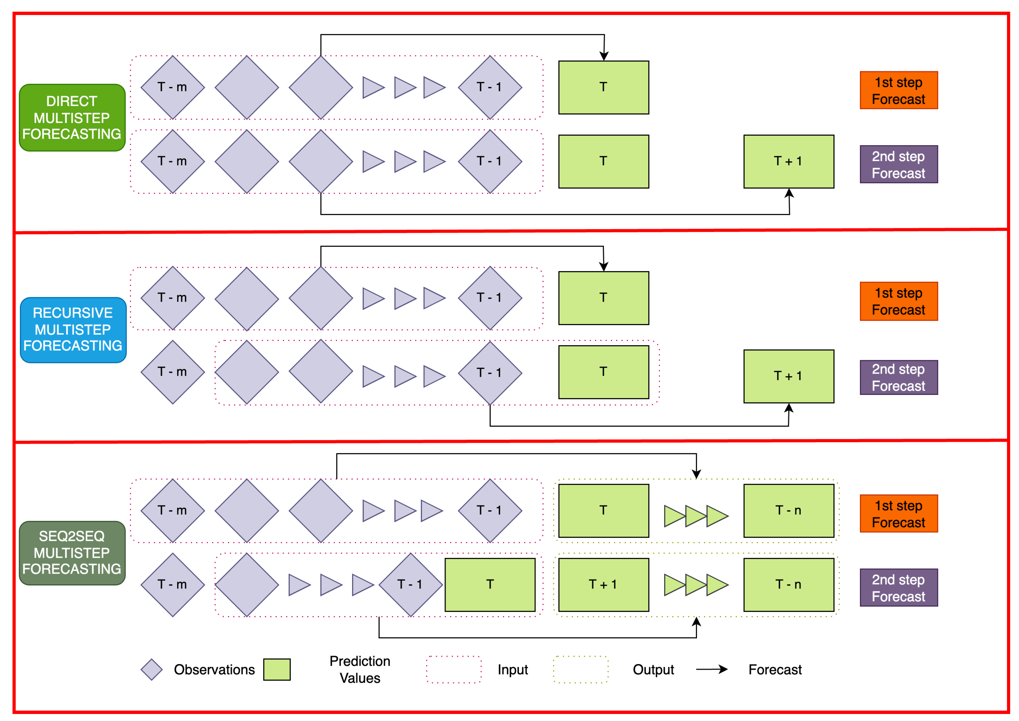
5.2. One-Step and Multistep-Ahead Forecasting

While one-step-ahead forecasting predicts a single future value, the objective of multistep-ahead prediction is to predict a sequence of future values in a time series. Three main strategies are frequently implemented for multistep forecasting (Figure 4): sequence-to-sequence models [127,128], direct models, and the rolling (or recursive) strategy [129].
Furthermore, considering Figure 4, it is notable to mention the following:
  • Direct Forecasting: With this approach, target values are predicted for each new step without considering previously estimated values. Though it is a straightforward approach, it can be hampered by a build-up of mistakes [21,130].
  • Recursive Forecasting: Also called rolling, this method predicts the values for the subsequent step using the expected values from the previous phases as inputs. In an iterative process, each anticipated value acts as an input for the prediction afterwards. Intertemporal dependencies may be more easily identified using this technique [21,129].
  • Sequence-to-Sequence Forecasting: A model is trained to convert an input sequence of historical values into an output sequence of values anticipated from a future perspective in sequence-to-sequence (seq2seq) forecasting. Sequential data are processed with transformers or RNNs. Sequence-to-sequence models are useful for long-term forecasting because of their ability to capture complex temporal trends [127].

6. Evaluation Metrics

A series of metrics can be used evaluate the results of EF algorithms and techniques to compare them. Selecting appropriate metrics to assess model performance is important but often neglected. Not all metrics are equal or capture predictive accuracy variations. Common metrics like the ones presented in this section can help identify prediction errors, but they may not meet energy forecasting applications’ needs. Emphasising the importance of determining which metrics best match forecasting task objectives and constraints is critical. Stakeholders can make better model selection and deployment decisions by prioritising metrics that best reflect forecast error consequences, such as financial or operational impacts.
Consequently, to aid in picking the best-suited common EF evaluation metrics, their mathematical formulations and brief descriptions/characteristics follow below.

6.1. Coefficient of Determination ( R 2 )

R-squared or R 2 constitutes the comparison of the variance of the error to the variance of the data that are to be modelled. In other words, it describes the proportion of variance ‘explained’ by the forecasting model, and therefore, unlike the following error-based metrics, the higher its value, the better the fit. It can be calculated as follows (Equation (1)):
R 2 = 1 S S r e s S S t o t = 1 ( y i f i ) 2 ( y i y ¯ ) 2
where S S r e s is the sum of squares of residuals (errors), and S S t o t is the total sum of squares (proportional to the variance of the data), y i is the actual power load value, y ¯ is the mean of the actual values, and f i is the forecasted value of the power load.

6.2. Mean Absolute Error (MAE)

The calculation of M A E is relatively simple (Equation (2)) since it only involves summing the absolute values of the errors (which is the difference between the actual and predicted values) and then dividing the total error by the number of observations. Unlike other statistical methods, the MAE applies the same weight to all errors.
M A E = 1 N i = 1 N | y i f i |
where y i is the actual value and f i is the forecasted value of the power load, and N is the number of values.

6.3. Mean Absolute Percentage Error (MAPE)

Another indicator of the accuracy of a regression model is the M A P E , which is extensively used, as it intuitively presents the error in terms of percentages. Its formula can be extracted by dividing each residual by the actual value in the formula of M A E (Equation (3)). However, this poses a serious problem when that actual value is zero or close to zero since this would lead to infinite M A P E or extremely high values, respectively.
M A P E = 1 N i = 1 N | y i f i | | y i |
where y i is the actual value and f i is the forecasted value of the power load, and N is the number of values.

6.4. Mean Squared Error (MSE)

The M S E indicates how good a fit is by calculating the squared difference between the i t h observed value and the corresponding model prediction and then finding the average of the set of errors (Equation (4)). The squaring, apart from removing any negative signs, also gives more weight to larger differences. It is clear that the lower the M S E , the better the forecast.
M S E = 1 N i = 1 N ( y i f i ) 2
where y i is the actual value and f i is the forecasted value of the power load, and N is the number of values.

6.5. Root Mean Squared Error (RMSE)

The R M S E is the square root of the average squared difference between the actual value and predicted value—in other words, the square root of the M S E . While these two metrics have very similar formulas (Equations (4) and (5)), the R M S E is more widely used since it is measured in the same units as the variable in question. The R M S E applies more weight to larger errors, taking into account that the impact of a single error on the total is proportional to its square and not its magnitude.
R M S E = 1 N i = 1 N ( y i f i ) 2

6.6. Coefficient of Variation of the Root Mean Squared Error (CVRMSE)

When normalising the RMSE by the mean value of the observations, another metric can be considered, the Coefficient of Variation of the Mean Squared Error ( C V R M S E ), thus resulting in the total error being expressed as a percentage (Equation (6)). According to their mathematical definitions, the R M S E and, consequently, the C V R M S E apply more weight to larger errors, given that the impact of a single error on the total is proportional to its square and not its magnitude.
C V R M S E ( % ) = R M S E y ¯ = ( y i f i ) 2 / N y i / N
where y i is the actual value, f i is the forecasted value of the power load, and N is the number of values. One significant advantage of the C V R M S E is that it is a dimensionless indicator, which can facilitate cross-study comparisons because it filters out the scale effect.

6.7. Normalised Root Mean Square Error (NRMSE)

The N R M S E is a measure that assesses the accuracy of a forecasting model by comparing anticipated and actual values. It is a standardised form of the R M S E that offers a comparative assessment of the model’s effectiveness (Equation (7)).
N R M S E = R M S E y i ( m a x ) y i ( m i n )
where y i ( m a x ) is the maximum observed value in the actual data, and y i ( m i n ) is the minimum observed value in the actual data. A lower N R M S E signifies a more accurate model alignment with the real data. It is commonly represented as a percentage by multiplying the outcome by 100.

6.8. Execution Time (ET)

ET typically measures the duration it takes for a model to process input data, train on them, and produce output predictions, most often reported in seconds. While being relevant, it is not a direct measure of the predictive accuracy and efficacy of a prediction model. Including ET as a core metric in a multi-measure model evaluation process can potentially overlook the model’s ability to capture important aspects, such as complex temporal patterns and seasonality, that may influence ELF or EGF. Moreover, ET can vary significantly depending on computational resources, hardware specifications, and software implementation details, making it difficult to standardise and compare across different studies. Consequently, although ET remains a substantial consideration for practical deployment and operational feasibility, it should be considered a supplementary or secondary metric when evaluating prediction models.

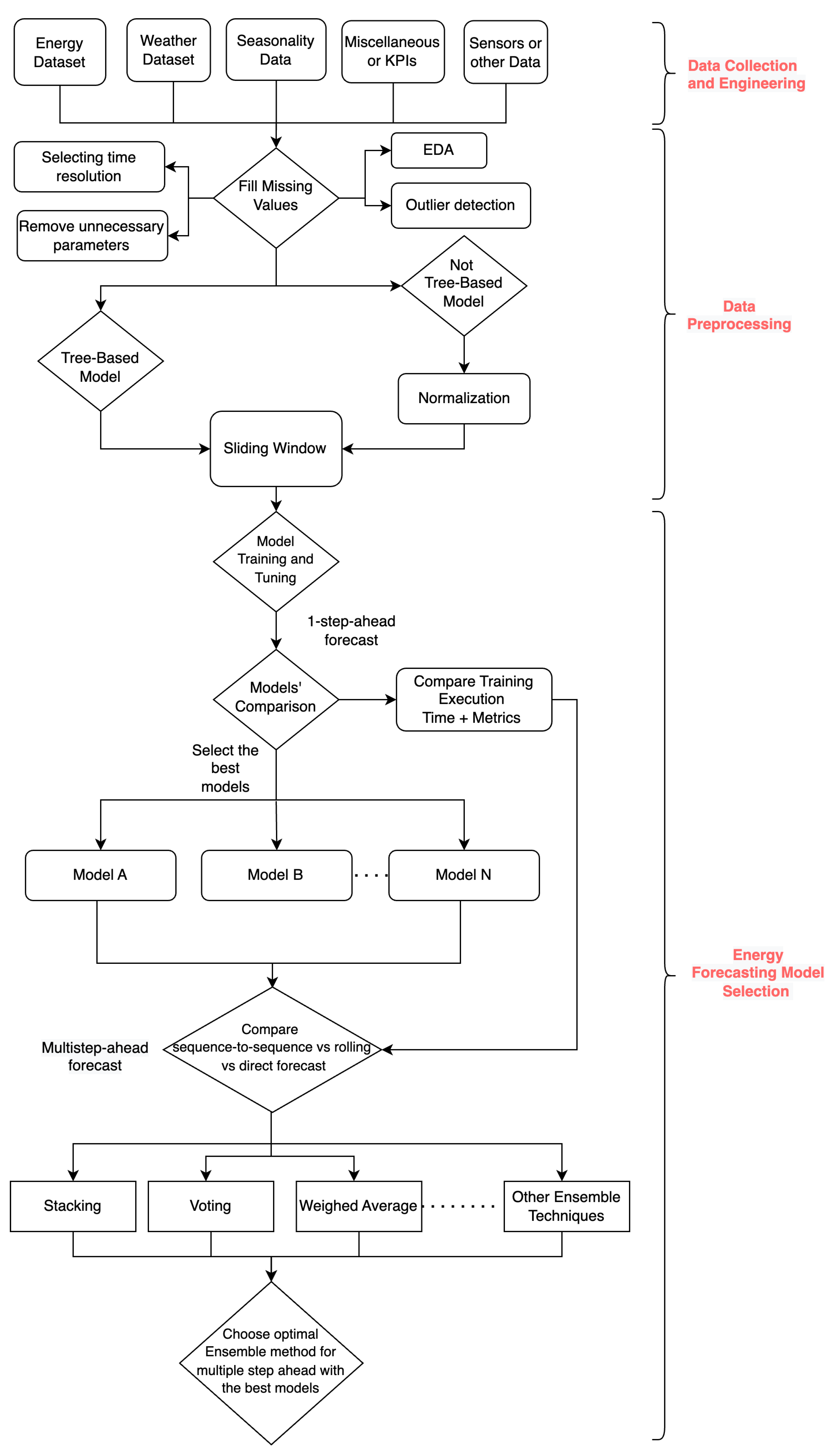
7. Standard Methodological Flow for Energy Forecasting

A generic flow for EF usually consists of three major steps. These include (i) data collection and engineering, (ii) data preprocessing, (iii) time-series regression for EF, as illustrated in Figure 5.

7.1. Data Collection and Engineering

In most cases, energy datasets are combined with other datasets from the same period, including weather, seasonality, sensors, KPIs, or miscellaneous information [21,22]. Such information may be modelled as a complex information network [131], and these different sources are usually combined via the data collection process, upgrading the problem from uni-variable to multi-variable.
To join all of these datasets, the time resolution should be the same (15 min, 30 min, 1 h, etc.), utilising rescaling methods [132]. Furthermore, a detailed Exploratory Data Analysis (EDA) is necessary, as John Tukey presented in his work [133], regarding the need for more integration between graphical analysis and descriptive measures. For these procedures, as well as for the next steps, several tools and technologies (among others) can be utilised, like MATLAB [134], SQL [135], or Python, along with frameworks such as Sklearn [132], Tensorflow [136], PyTorch [137], Pandas [138], Numpy [139], and Matplotlib [140], under different versions as the evolve through time.

7.2. Data Preprocessing

Several processes in the previous subsection, like EDA (possibly part of both subsections), outlier detection/removal, or the filling in of missing values, could also be said to belong to Section 7.1. The basic preprocessing techniques for EGF were classified into seven categories according to applications [141]: decomposition, feature selection, feature extraction, denoising, residual error modelling, outlier detection, and filter-based correction. However, the possible final combined dataset can be distinguished before these procedures, clearly showing all the values with their unique timestamps in the middle of the process (after EDA and before outlier detection/removal or filling missing values). Then, usually, the procedure continues on the transformed dataset that is ready to be used for training, testing, and validation [21].
A detailed EDA can provide important information about the final dataset, showing whether procedures like outlier detection/removal or the filling in of missing values are necessary [142]. EDA can also provide details on the feature selection procedure, as well as important information regarding the data quality of the selected dataset. In [143], investigations were conducted into the impact of various dataset-cleaning techniques on the accuracy of ELF. To find the outliers in the dataset, the Generalised Extreme Studentised Deviate (GESD) hypothesis test was implemented. Based on an autocorrelation analysis that revealed a weekly correlation between the samples, the populations were built, highlighting the significance of data processing before using them for EF.
Tree-based models and non-TBMs usually use rather different approaches after adding missing data and before implementing time-series regression techniques. The former does not require normalisation because of their description. The latter models possibly utilise this transformation, for example, via the MinMaxScaler function of the Python sklearn.preprocessing package [132], with the modified dataset falling within a specific range.
The SW [144] technique is utilised before the time-series regression execution. This involves number-step-ahead data shifting (for example, 24 h with 15 min resolution for a total of 96 steps), with the outcome becoming the input dataset for the models. RNN-based models utilise a three-dimensional SW (timesteps, rows, and parameters), whereas the remaining models proceed with a two-dimensional one (rows, parameters + timesteps). Next, the dataset is typically split into test and training sets, typically allocating 20% for testing and 80% for training (with some cases using another 5–10% for further validation) [145].

7.3. Time-Series Regression

Moving to the EF time-series regression part, a standard methodology includes the testing of several ML and DL algorithms (presented in Section 4) for one-step-ahead EGF or ELF. Only the top performers are chosen for additional research and hyperparameter tuning [146], with the evaluation being conducted using metrics like the ones in Section 6. An additional comparison is usually conducted to determine the optimal ensemble approach (Section 4.4) in conjunction with the optimal multistep strategy, as well as the ET. At the same time, the subsequent phase involves comparing these algorithms for a rolling versus direct versus seq2seq multistep strategy, as described in Section 5.
It is important to highlight that the standard methodology can vary depending on the models implemented, as well as the ensemble methods or multistep-ahead strategies utilised. For example, in a direct multistep-ahead forecasting implementation, there could be different models or different ensemble methods per timestep ahead or even a combination of them.

8. Discussion

In this comprehensive exploration of EF, this section discusses the diverse approaches for predicting energy trends, examines how pivotal and related EF advancements in technology influence forecasting accuracy, and exposes the obstacles in predicting energy requirements and their broader implications.

8.1. Methodologies in Energy Forecasting

This paper provides an overview of the methodologies that constitute the foundation of EF, including statistical, ML, and DL algorithms and several ensemble methods. It examines several time-series forecasting methods, such as direct, recursive, and sequence-to-sequence. It discusses the metrics, both relative (including the ET) and absolute, used to measure the accuracy of predictions, like M A E , R M S E , R 2 , and C V R M S E . It offers a comprehensive, step-by-step standard methodology that is frequently applied to the majority of EF procedures.
The evolution of energy forecasting methodologies has been significantly influenced by the integration of ML and DL techniques, moving beyond the confines of traditional statistical approaches. This transition is marked by the adoption of LR models, which serve as a foundation for both statistical and ML models in energy forecasting. The extension of LR with periodic components to address non-stationary time series highlights the adaptability of these models to complex energy patterns [73,74]. The development of regularised forms of LR, such as Ridge Regression (RR) and Lasso Regression, underscores efforts to mitigate overfitting, enhancing model robustness and prediction accuracy [75]. SVR, with its high-dimensional feature space, exemplifies the sophistication of ML techniques in handling complex energy datasets [76,77]. Moreover, this review provides some general highlights of how the EF research field is shifting. For example, the use of standalone statistical approaches is decreasing, especially for VSTF and STF. Recent works have shown that statistical models work either as part of an ensemble method [48] or for MTF and LTF applications [62].
It was also noted that, due to the nature of energy datasets [21,22] and the performance of TBMs on data with zero values, there is an increase in TBM usage on EF problems. The capability of TBMs to manage outliers and nonlinear relationships between attributes and the target variable has been a significant advantage [82,83,84,85,86]. Among TBMs, RF and Extremely Randomised Trees (Extra-Trees) illustrate the ensemble approach’s strength in reducing overfitting through the Law of Large Numbers and introducing randomness into the model selection process [88,89]. This information, combined with the development of more powerful and accurate boosting models (as an extension of TBMs) like LGBMR [95], HGBR [91], and CBR [96], led to an increase in TBM applications to EGF and ELF.
Other boosting models, as extensions of TBMs, can further enhance forecasting performance by sequentially correcting previous predictors. GBR and XGBR are notable for their efficacy in simulating energy use in commercial buildings and achieving state-of-the-art results across various ML problems [90,91,92,93,94].
DL regression models, including FNNs, RNNs, LSTM networks, and CNNs, represent advanced methodologies that are also capable of capturing complex temporal and spatial relationships in energy data [98,99,100,101,103,104,105,106,107,108]. These models’ ability to process large data series and their suitability for various applications, from natural language processing to image classification, underscore DL’s transformative impact on energy forecasting.
It was also highlighted that ensemble methods, leveraging the strengths of multiple forecasting models, have shown significant promise in improving prediction accuracy. Techniques ranging from the BEM to the GEM and dynamically weighted ensembles highlight the diversity and potential of ensemble approaches in energy forecasting [111,112,113,114,115,116,117,118]. These methods, through the strategic combination and weighting of models, aim to reduce bias and variance, presenting a comprehensive approach to tackling the intricacies of energy forecasting challenges.

8.2. Impact of Computing Power and Data Complexity

Another aspect discussed is the increased computing power and data complexity in the last decade. Data management systems, IoT devices, and advanced hardware have also impacted the EF research field. Many VSTF case studies [21] made it necessary to develop more complicated models like DL algorithms, which need a lot of resources and are hard to understand [11,103].
Besides the general increase in EF research over the last years, there are more and more works that combine ELF and EGF research with DR, proactive planning, efficient resource allocation, and grid integration of renewable energy sources [2]. The information that these estimates provide is crucial for decision-makers in several industries, including industry, government, utilities, and SC.

8.3. Challenges and Implications of Energy Forecasting

The limitations of this work can be attributed to the extension and the size of EF as a field of study and research. Although many concepts and original and state-of-the-art algorithms and methodologies are presented in this work, the research field of EF has massively increased over the last years, making it impossible to cover every aspect of it, as shown by the bibliometrics of the current research in Figure 6. Thus, this figure contains information based on the structured research progression presented in Section 2.3.
The main challenges and implications of EF can be broken down into the following categories:
  • Data Quality: High-quality data are the cornerstone of accurate forecasting. However, issues such as missing values, inaccuracies, and inconsistencies within datasets can severely affect the performance of forecasting models. The complexity and variability of energy data further exacerbate these issues, necessitating sophisticated data preprocessing techniques to ensure reliability and accuracy in forecasting outcomes. Algorithms and anomaly detection techniques are often employed to address these challenges, enabling researchers and practitioners to mitigate the impact of data quality issues and enhance the robustness of forecasting models for both ELF [143] and EGF [141].
  • Model Complexity: The increasing sophistication of EF models, especially with the adoption of advanced ML and DL techniques, introduces complexities in model development, interpretation, and implementation. While these models significantly improve forecasting accuracy, their complexity can pose challenges regarding computational demands, model transparency, and the expertise required for effective application and maintenance.
  • Adaptability to Rapidly Evolving Energy Landscapes and Market Trends: The energy sector is undergoing rapid transformations driven by the integration of renewable energy sources, changes in consumption patterns, and regulatory shifts. Forecasting models must be adaptable to these changes, capable of incorporating new data sources, and flexible enough to adjust to new market dynamics and policy requirements. In more detail, traditional forecasting methods must adapt to the intermittent nature of RESs like solar and wind and their impact on EGF. New consumer choices and technology, such as electric vehicles and smart home devices, affect EED and consumption patterns. Regulations forcing carbon pricing mechanisms and energy efficiency rules change the energy sector’s economic landscape, affecting investment and market behaviour. To remain timely and efficient in these dynamic energy environments, EF models must be continuously reviewed and revised to match market needs.
  • Ethical Concerns, Data Privacy, and Security: Ensuring the confidentiality and protection of energy-related data during their collection and processing is of paramount importance. The improper or illegal utilisation of sensitive energy data raises problems regarding privacy and confidentiality. Cyberattacks, data breaches, and malicious acts can impact vital infrastructure and energy systems. Encryption, access restrictions, and anonymisation are essential for mitigating dangers and safeguarding energy data. Therefore, appropriate regulations governing the collection, storage, sharing, and exploitation of energy data should be enforced, seeking a balance between using data-derived insights, addressing ethical concerns, and safeguarding privacy and security rights.
The methodological implications of these challenges extend beyond the technical aspects of EF, affecting industry practices, policy-making, and strategic planning. Addressing these challenges is crucial for advancing the field of EF and ensuring that forecasting models can effectively support decision-making processes in a rapidly evolving energy sector.

9. Conclusions

The study thoroughly examines statistical, ML, and DL techniques in the EF field, highlighting both traditional and cutting-edge methods that advance the industry. It analyses the latest advancements in ELF and EGF, covering various techniques from traditional statistical models to advanced DL algorithms and their ensemble applications. The overview provided outlines the development of forecasting approaches and emphasises the importance of following a thorough standard methodology. Therefore, the main objective was to synthesise and analyse the current literature and provide a thorough comprehension and assessment of forecasting techniques and technologies. This was achieved by summarising important observations, pinpointing areas where further investigation is needed, and indicating future research directions.
The conducted analysis suggested that practical implementation examples may differ significantly depending on specific application domains, dataset characteristics/features, and operational contexts. This variability makes it challenging to generalise findings across diverse scenarios. Consequently, although practical examples of implementation may be valuable for illustrating the applicability of certain techniques, this work does not provide detailed results on certain approaches or case studies of research papers. In contrast, it reviews the techniques and technologies related to EF.
In addition, the examination showed an interest in methodological advancements related to extremely short-term and short-term forecasting. The transition is mainly due to the increasing data and complexity, which require sophisticated computational models to estimate energy consumption and generation effectively. The increasing use of TBMs and ensemble methods in forecasting processes highlights the industry’s emphasis on precision and resilience.
This review combined many crucial techniques in developing EF research. It underscored technological development and the increasing intricacy and specialisation of forecasting requirements. The findings from this thorough analysis act as a guide for upcoming investigations, highlighting the importance of ongoing innovation and adjustment in response to changing energy prediction difficulties.

Future Directions

Future research in EF should aim to enhance data preprocessing methods, develop more interpretable and less computationally demanding models, and increase the adaptability of forecasting techniques. Addressing these concerns could help accommodate the dynamic nature of the energy landscape, creating more sustainable, efficient, and resilient energy systems. This study could be enhanced by investigating the following aspects:
  • In the context of multistep-ahead forecasting, it would be beneficial to identify the best strategy, i.e., direct versus recursive versus seq2seq, depending on the energy type. For example, heating, cooling, and electricity are used for ELF, and solar, wind, and hydroelectric power are used for EGF.
  • Possible methodologies that could use an ensemble method combined with a multistep-ahead strategy could be identified so as to cover all energy types utilising a combined dataset.
  • Any other beneficial input features/parameters outside of the standard mentioned in Section 3.1 could be recognised so as to boost the performance of EF models.
  • To address new energy load or generation types with distinct characteristics, such as the EV charging load or geothermal generation inside the EF framework, their integration with the prior step (identifying any additional advantageous input features/parameters) could be considered. For example, in the field of Smart Cities, urban traffic congestion data can be used to predict future events and anticipate the load for electric vehicle charging.
  • Investigating the application of advanced artificial intelligence techniques, including ML and DL, which represent untapped potential for enhancing EF, for real-time, adaptive forecasting models could revolutionise energy management systems, providing more accurate and timely predictions to support decision-making processes. These could include optimisation procedures such as linear [147], integer [148], dynamic [149], or mixed-integer linear [150] programming by using optimisation libraries and software systems like CPLEX [151] or Gurobi, (in their latest versions) [152] after processing the results of accurate EF.

Author Contributions

Conceptualisation, A.M. and P.K.; methodology, A.M. and P.K.; formal analysis, A.M.; validation, A.M., P.K., N.T. and C.T.; writing—original draft preparation, A.M. and P.K.; writing—review and editing, A.M., N.T., P.K. and C.T.; supervision, P.K., D.I. and C.T.; project administration/resources P.K., D.I. and C.T.; funding acquisition, C.T. All authors have read and agreed to the published version of the manuscript.

Funding

This research received no external funding.

Conflicts of Interest

The authors declare no conflicts of interest.

Abbreviations

The following abbreviations are used in this manuscript:
ABRAdaBoost Regressor
ANNArtificial Neural Networks
ARXAuto-Regressive model with eXtra inputs
BEMBasic Ensemble Method
Bi-LSTMBi-directional Long Short-Term Memory
BRRBayesian Ridge Regression
CBRCategorical Boosting Regressor
CNNConvolutional Neural Networks
CVRMSECoefficient of Variation of the Root Mean Squared Error
DBNDeep Belief Network
DLDeep Learning
DNNDeep Neural Networks
DRDemand Response
DRMDemand Response Management
DSODistribution System Operator
DTDecision tree
EEDElectrical Energy Demand
EEDiEnergy Efficiency Directive
EFEnergy forecasting
EGFEnergy Generation Forecasting
ELFEnergy Load Forecasting
ELMExtreme Learning Machine
ENElastic Net
ENRElastic Net Regression
EPMsEnergy Planning Models
ETExecution Time
ETSExponential smoothing
FNNFeedforward Neural Networks
GBRGradient Boosting Regressor
GEMGeneralised Ensemble Technique
GESDGeneralized Extreme Studentized Deviate
GPsGaussian Processes
GRUGated Recurrent Unit
GWOGrey Wolf Optimisation
HGBRHistogram-Based Gradient Boosting Regressor
HVACHeating, Ventilation, and Air Conditioning
IoTInternet of Things
KPIsKey Performance Indicators
LGBMRLight Gradient Boosting Machine Regressor
LPLog-normal Process
LRLinear Regression
LSRLasso Regression
LSTMLong Short-Term Memory
LTFLong-Term Forecasting
LTGFLong-Term Generation Forecasting
LTLFLong-Term Load Forecasting
MAEMean Absolute Error
MAPEMean Absolute Percentage Error
MEFMonthly Energy Forecasting
MIMutual Information
MLMachine Learning
MLPMulti-layer Perceptron
MLRMultiple Linear Regression
MSEMean Squared Error
MTFMedium-Term Forecasting
MTGFMedium Term Generation Forecasting
MTLFMedium Term Load Forecasting
NNsNeural Networks
NRMSENormalised Root Mean Squared Error
NWPNumerical Weather Prediction
PRPolynomial Regression
PSOParticle Swarm Optimisation
PVPhotovoltaic
RBFNRadial Basis Function Networks
RFRandom Forest
RLReinforcement Learning
RMSERoot Mean Squared Error
RNNRecurrent Neural Networks
RODDPSORandomly Occurring Distributedly Delayed Particle Swarm Optimisation
RRRidge Regression
SCSmart Cities
SGSmart Grid
STFShort-Term Forecasting
STGFShort-Term Generation Forecasting
STLFShort-Term Load Forecasting
SVMSupport Vector Machine
SVRSupport Vector Regression
SWSliding Window
TBMsTree-based models
VSTFVery Short-Term Forecasting
VSTGFVery Short-Term Generation Forecasting
VSTLFVery Short-Term Load Forecasting
WTWavelet Transformation
XGBRExtreme Gradient Boosting Regressor
ZIZero-Inflated
ZICClassification Part of Ensemble Zero-Inflated Regression
ZIRRegression Part of Ensemble Zero-Inflated Regression

References

  1. Coakley, D.; Raftery, P.; Keane, M. A review of methods to match building energy simulation models to measured data. Renew. Sustain. Energy Rev. 2014, 37, 123–141. [Google Scholar] [CrossRef]
  2. Singh Aujla, G.; Garg, S.; Batra, S.; Kumar, N.; You, I.; Sharma, V. DROpS: A demand response optimization scheme in SDN-enabled smart energy ecosystem. Inf. Sci. 2019, 476, 453–473. [Google Scholar] [CrossRef]
  3. Fallah, S.N.; Deo, R.C.; Shojafar, M.; Conti, M.; Shamshirband, S. Computational Intelligence Approaches for Energy Load Forecasting in Smart Energy Management Grids: State of the Art, Future Challenges, and Research Directions. Energies 2018, 11, 596. [Google Scholar] [CrossRef]
  4. Koukaras, P.; Gkaidatzis, P.; Bezas, N.; Bragatto, T.; Carere, F.; Santori, F.; Antal, M.; Ioannidis, D.; Tjortjis, C.; Tzovaras, D. A tri-layer optimization framework for day-ahead energy scheduling based on cost and discomfort minimization. Energies 2021, 14, 3599. [Google Scholar] [CrossRef]
  5. Koukaras, P.; Tjortjis, C.; Gkaidatzis, P.; Bezas, N.; Ioannidis, D.; Tzovaras, D. An interdisciplinary approach on efficient virtual microgrid to virtual microgrid energy balancing incorporating data preprocessing techniques. Computing 2022, 104, 209–250. [Google Scholar] [CrossRef]
  6. Maçaira, P.; Elsland, R.; Oliveira, F.C.; Souza, R.; Fernandes, G. Forecasting residential electricity consumption: A bottom-up approach for Brazil by region. Energy Effic. 2020, 13, 911–934. [Google Scholar] [CrossRef]
  7. Eder, L.; Provornaya, I. Analysis of energy intensity trend as a tool for long-term forecasting of energy consumption. Energy Effic. 2018, 11, 1971–1997. [Google Scholar] [CrossRef]
  8. Mahendra, L.; Kalluri, R.; Rao, M.S.; Kumar, R.S.; Bindhumadhava, B. Leveraging forecasting techniques for power procurement and improving grid stability: A strategic approach. In Proceedings of the 2017 IEEE PES Asia-Pacific Power and Energy Engineering Conference (APPEEC), Bangalore, India, 8–10 November 2017; IEEE: Piscataway, NJ, USA, 2017; pp. 1–6. [Google Scholar]
  9. Kumar, C.J.; Veerakumari, M. Load forecasting of Andhra Pradesh grid using PSO, DE algorithms. Int. J. Adv. Res. Comput. Eng. Technol. 2012, 1, 179–184. Available online: https://api.semanticscholar.org/CorpusID:11930759 (accessed on 2 March 2024).
  10. Yang, Y.; Wang, Z.; Gao, Y.; Wu, J.; Zhao, S.; Ding, Z. An effective dimensionality reduction approach for short-term load forecasting. Electr. Power Syst. Res. 2022, 210, 108150. [Google Scholar] [CrossRef]
  11. Hammad, M.A.; Jereb, B.; Rosi, B.; Dragan, D. Methods and Models for Electric Load Forecasting: A Comprehensive Review. Logist. Supply Chain. Sustain. Glob. Chall. 2020, 11, 51–76. [Google Scholar] [CrossRef]
  12. Subbiah, S.S.; Chinnappan, J. Deep learning based short term load forecasting with hybrid feature selection. Electr. Power Syst. Res. 2022, 210, 108065. [Google Scholar] [CrossRef]
  13. Khwaja, A.; Anpalagan, A.; Naeem, M.; Venkatesh, B. Joint bagged-boosted artificial neural networks: Using ensemble machine learning to improve short-term electricity load forecasting. Electr. Power Syst. Res. 2020, 179, 106080. [Google Scholar] [CrossRef]
  14. Kuo, P.H.; Huang, C.J. A High Precision Artificial Neural Networks Model for Short-Term Energy Load Forecasting. Energies 2018, 11, 213. [Google Scholar] [CrossRef]
  15. Raza, M.Q.; Khosravi, A. A review on artificial intelligence based load demand forecasting techniques for smart grid and buildings. Renew. Sustain. Energy Rev. 2015, 50, 1352–1372. [Google Scholar] [CrossRef]
  16. Singh, A.K.; Ibraheem; Khatoon, S.; Muazzam, M.; Chaturvedi, D.K. Load forecasting techniques and methodologies: A review. In Proceedings of the 2012 2nd International Conference on Power, Control and Embedded Systems, Allahabad, India, 17–19 December 2012; pp. 1–10. [Google Scholar] [CrossRef]
  17. Nti, I.K.; Teimeh, M.; Nyarko-Boateng, O.; Adekoya, A.F. Electricity load forecasting: A systematic review. J. Electr. Syst. Inf. Technol. 2020, 7, 13. [Google Scholar] [CrossRef]
  18. Ding, S.; Li, R.; Tao, Z. A novel adaptive discrete grey model with time-varying parameters for long-term photovoltaic power generation forecasting. Energy Convers. Manag. 2021, 227, 113644. [Google Scholar] [CrossRef]
  19. Das, U.K.; Tey, K.S.; Seyedmahmoudian, M.; Mekhilef, S.; Idris, M.Y.I.; Van Deventer, W.; Horan, B.; Stojcevski, A. Forecasting of photovoltaic power generation and model optimization: A review. Renew. Sustain. Energy Rev. 2018, 81, 912–928. [Google Scholar] [CrossRef]
  20. Barbosa de Alencar, D.; de Mattos Affonso, C.; Limão de Oliveira, R.C.; Moya Rodriguez, J.L.; Leite, J.C.; Reston Filho, J.C. Different models for forecasting wind power generation: Case study. Energies 2017, 10, 1976. [Google Scholar] [CrossRef]
  21. Mystakidis, A.; Ntozi, E.; Afentoulis, K.; Koukaras, P.; Gkaidatzis, P.; Ioannidis, D.; Tjortjis, C.; Tzovaras, D. Energy generation forecasting: Elevating performance with machine and deep learning. Computing 2023, 105, 1623–1645. [Google Scholar] [CrossRef]
  22. Mystakidis, A.; Ntozi, E.; Afentoulis, K.; Koukaras, P.; Giannopoulos, G.; Bezas, N.; Gkaidatzis, P.A.; Ioannidis, D.; Tjortjis, C.; Tzovaras, D. One Step Ahead Energy Load Forecasting: A Multi-model approach utilizing Machine and Deep Learning. In Proceedings of the 2022 57th International Universities Power Engineering Conference (UPEC), Istanbul, Turkey, 30 August–2 September 2022; pp. 1–6. [Google Scholar] [CrossRef]
  23. Debnath, K.B.; Mourshed, M. Forecasting methods in energy planning models. Renew. Sustain. Energy Rev. 2018, 88, 297–325. [Google Scholar] [CrossRef]
  24. Chammas, M.; Makhoul, A.; Demerjian, J. An efficient data model for energy prediction using wireless sensors. Comput. Electr. Eng. 2019, 76, 249–257. [Google Scholar] [CrossRef]
  25. Klyuev, R.V.; Morgoeva, A.D.; Gavrina, O.A.; Bosikov, I.I.; Morgoev, I.D. Forecasting planned electricity consumption for the united power system using machine learning. J. Min. Inst. 2023, 261, 392–402. [Google Scholar]
  26. Chalal, M.L.; Benachir, M.; White, M.; Shrahily, R. Energy planning and forecasting approaches for supporting physical improvement strategies in the building sector: A review. Renew. Sustain. Energy Rev. 2016, 64, 761–776. [Google Scholar] [CrossRef]
  27. Zangheri, P.; Armani, R.; Pietrobon, M.; Pagliano, L.; Boneta, M.F.; Müller, A. Heating and cooling energy demand and loads for building types in different countries of the EU. Polytech. Univ. Turin End-Use Effic. Res. Group 2014, 3, 1–86. Available online: https://www.entranze.eu/files/downloads/ (accessed on 2 March 2024).
  28. Koohi-Fayegh, S.; Rosen, M.A. A review of energy storage types, applications and recent developments. J. Energy Storage 2020, 27, 101047. Available online: https://api.semanticscholar.org/CorpusID:210616155 (accessed on 2 March 2024). [CrossRef]
  29. Wang, Z.; Hong, T.; Piette, M.A. Building thermal load prediction through shallow machine learning and deep learning. Appl. Energy 2020, 263, 114683. [Google Scholar] [CrossRef]
  30. Ahmad, A.; Javaid, N.; Mateen, A.; Awais, M.; Khan, Z.A. Short-Term Load Forecasting in Smart Grids: An Intelligent Modular Approach. Energies 2019, 12, 164. [Google Scholar] [CrossRef]
  31. Fu, G. Deep belief network based ensemble approach for cooling load forecasting of air-conditioning system. Energy 2018, 148, 269–282. [Google Scholar] [CrossRef]
  32. Deng, X.; Ye, A.; Zhong, J.; Xu, D.; Yang, W.; Song, Z.; Zhang, Z.; Guo, J.; Wang, T.; Tian, Y.; et al. Bagging–XGBoost algorithm based extreme weather identification and short-term load forecasting model. Energy Rep. 2022, 8, 8661–8674. [Google Scholar] [CrossRef]
  33. Sekhar, C.; Dahiya, R. Robust framework based on hybrid deep learning approach for short term load forecasting of building electricity demand. Energy 2023, 268, 126660. [Google Scholar] [CrossRef]
  34. Zhuang, D.; Gan, V.J.; Tekler, Z.D.; Chong, A.; Tian, S.; Shi, X. Data-driven predictive control for smart HVAC system in IoT-integrated buildings with time-series forecasting and reinforcement learning. Appl. Energy 2023, 338, 120936. [Google Scholar] [CrossRef]
  35. Wan, A.; Chang, Q.; Khalil, A.B.; He, J. Short-term power load forecasting for combined heat and power using CNN-LSTM enhanced by attention mechanism. Energy 2023, 282, 128274. [Google Scholar] [CrossRef]
  36. Nti, I.; Asafo-Adjei, S.; Agyemang, M. Predicting monthly electricity demand using soft-computing technique. Int. Res. J. Eng. Technol. 2019, 6, 1967–1973. Available online: https://www.irjet.net/archives/V6/i6/IRJET-V6I6428.pdf (accessed on 2 March 2024).
  37. Tanaka, K.; Uchida, K.; Ogimi, K.; Goya, T.; Yona, A.; Senjyu, T.; Funabashi, T.; Kim, C.H. Optimal operation by controllable loads based on smart grid topology considering insolation forecasted error. IEEE Trans. Smart Grid 2011, 2, 438–444. [Google Scholar] [CrossRef]
  38. Kudo, M.; Takeuchi, A.; Nozaki, Y.; Endo, H.; Sumita, J. Forecasting electric power generation in a photovoltaic power system for an energy network. Electr. Eng. Jpn. 2009, 167, 16–23. [Google Scholar] [CrossRef]
  39. Gigoni, L.; Betti, A.; Crisostomi, E.; Franco, A.; Tucci, M.; Bizzarri, F.; Mucci, D. Day-ahead hourly forecasting of power generation from photovoltaic plants. IEEE Trans. Sustain. Energy 2017, 9, 831–842. [Google Scholar] [CrossRef]
  40. Liu, L.; Zhan, M.; Bai, Y. A recursive ensemble model for forecasting the power output of photovoltaic systems. Sol. Energy 2019, 189, 291–298. [Google Scholar] [CrossRef]
  41. Visser, L.; AlSkaif, T.; Van Sark, W. Benchmark analysis of day-ahead solar power forecasting techniques using weather predictions. In Proceedings of the 2019 IEEE 46th Photovoltaic Specialists Conference (PVSC), Chicago, IL, USA, 16–21 June 2019; IEEE: Piscataway, NJ, USA, 2019; pp. 2111–2116. [Google Scholar] [CrossRef]
  42. Al-Mejibli, I.S.; Alwan, J.K.; Abd Dhafar, H. The effect of gamma value on support vector machine performance with different kernels. Int. J. Electr. Comput. Eng. 2020, 10, 5497. [Google Scholar] [CrossRef]
  43. Pan, M.; Li, C.; Gao, R.; Huang, Y.; You, H.; Gu, T.; Qin, F. Photovoltaic power forecasting based on a support vector machine with improved ant colony optimization. J. Clean. Prod. 2020, 277, 123948. [Google Scholar] [CrossRef]
  44. Zhou, Y.; Zhou, N.; Gong, L.; Jiang, M. Prediction of photovoltaic power output based on similar day analysis, genetic algorithm and extreme learning machine. Energy 2020, 204, 117894. [Google Scholar] [CrossRef]
  45. Liu, Z.F.; Li, L.L.; Tseng, M.L.; Lim, M.K. Prediction short-term photovoltaic power using improved chicken swarm optimizer-extreme learning machine model. J. Clean. Prod. 2020, 248, 119272. [Google Scholar] [CrossRef]
  46. Zheng, J.; Zhang, H.; Dai, Y.; Wang, B.; Zheng, T.; Liao, Q.; Liang, Y.; Zhang, F.; Song, X. Time series prediction for output of multi-region solar power plants. Appl. Energy 2020, 257, 114001. [Google Scholar] [CrossRef]
  47. Jallal, M.A.; Chabaa, S.; Zeroual, A. A novel deep neural network based on randomly occurring distributed delayed PSO algorithm for monitoring the energy produced by four dual-axis solar trackers. Renew. Energy 2020, 149, 1182–1196. [Google Scholar] [CrossRef]
  48. Sharadga, H.; Hajimirza, S.; Balog, R.S. Time series forecasting of solar power generation for large-scale photovoltaic plants. Renew. Energy 2020, 150, 797–807. [Google Scholar] [CrossRef]
  49. Chang, G.W.; Lu, H.J. Integrating gray data preprocessor and deep belief network for day-ahead PV power output forecast. IEEE Trans. Sustain. Energy 2018, 11, 185–194. [Google Scholar] [CrossRef]
  50. Ojha, V.K.; Abraham, A.; Snášel, V. Metaheuristic design of feedforward neural networks: A review of two decades of research. Eng. Appl. Artif. Intell. 2017, 60, 97–116. [Google Scholar] [CrossRef]
  51. Mayer, M.J. Benefits of physical and machine learning hybridization for photovoltaic power forecasting. Renew. Sustain. Energy Rev. 2022, 168, 112772. [Google Scholar] [CrossRef]
  52. Essam, Y.; Ahmed, A.N.; Ramli, R.; Chau, K.W.; Ibrahim, M.S.I.; Sherif, M.; Sefelnasr, A.; El-Shafie, A. Investigating photovoltaic solar power output forecasting using machine learning algorithms. Eng. Appl. Comput. Fluid Mech. 2022, 16, 2002–2034. [Google Scholar] [CrossRef]
  53. Zheng, J.; Du, J.; Wang, B.; Klemeš, J.J.; Liao, Q.; Liang, Y. A hybrid framework for forecasting power generation of multiple renewable energy sources. Renew. Sustain. Energy Rev. 2023, 172, 113046. [Google Scholar] [CrossRef]
  54. Shepero, M.; Van Der Meer, D.; Munkhammar, J.; Widén, J. Residential probabilistic load forecasting: A method using Gaussian process designed for electric load data. Appl. Energy 2018, 218, 159–172. [Google Scholar] [CrossRef]
  55. Dogan, E. Are shocks to electricity consumption transitory or permanent? Sub-national evidence from Turkey. Util. Policy 2016, 41, 77–84. [Google Scholar] [CrossRef]
  56. Pełka, P.; Dudek, G. Prediction of monthly electric energy consumption using pattern-based fuzzy nearest neighbour regression. ITM Web Conf. 2017, 15, 02005. [Google Scholar] [CrossRef]
  57. Pełka, P.; Dudek, G. Ensemble forecasting of monthly electricity demand using pattern similarity-based methods. In Proceedings of the International Conference on Artificial Intelligence and Soft Computing, Zakopane, Poland, 12 October 2020; Springer: Berlin/Heidelberg, Germany, 2020; pp. 712–723. [Google Scholar] [CrossRef]
  58. Castán-Lascorz, M.; Jiménez-Herrera, P.; Troncoso, A.; Asencio-Cortés, G. A new hybrid method for predicting univariate and multivariate time series based on pattern forecasting. Inf. Sci. 2021, 586, 611–627. [Google Scholar] [CrossRef]
  59. Bunnoon, P.; Chalermyanont, K.; Limsakul, C. Mid term load forecasting of the country using statistical methodology: Case study in Thailand. In Proceedings of the 2009 International conference on signal processing systems, Singapore, 15–17 May 2009; IEEE: Piscataway, NJ, USA, 2009; pp. 924–928. [Google Scholar] [CrossRef]
  60. Hyndman, R.; Koehler, A.B.; Ord, J.K.; Snyder, R.D. Forecasting with Exponential Smoothing: The State Space Approach; Springer Science & Business Media: Berlin, Germany, 2008. [Google Scholar] [CrossRef]
  61. Papalexopoulos, A.D.; Hesterberg, T.C. A regression-based approach to short-term system load forecasting. IEEE Trans. Power Syst. 1990, 5, 1535–1547. [Google Scholar] [CrossRef]
  62. de Oliveira, E.M.; Oliveira, F.L.C. Forecasting mid-long term electric energy consumption through bagging ARIMA and exponential smoothing methods. Energy 2018, 144, 776–788. [Google Scholar] [CrossRef]
  63. Maltais, L.G.; Gosselin, L. Forecasting of short-term lighting and plug load electricity consumption in single residential units: Development and assessment of data-driven models for different horizons. Appl. Energy 2022, 307, 118229. [Google Scholar] [CrossRef]
  64. Lin, J.; Fernández, J.A.; Rayhana, R.; Zaji, A.; Zhang, R.; Herrera, O.E.; Liu, Z.; Mérida, W. Predictive analytics for building power demand: Day-ahead forecasting and anomaly prediction. Energy Build. 2022, 255, 111670. [Google Scholar] [CrossRef]
  65. Pfafferott, J.; Herkel, S.; Wapler, J. Thermal building behaviour in summer: Long-term data evaluation using simplified models. Energy Build. 2005, 37, 844–852. [Google Scholar] [CrossRef]
  66. Cho, S.H.; Kim, W.T.; Tae, C.S.; Zaheeruddin, M. Effect of length of measurement period on accuracy of predicted annual heating energy consumption of buildings. Energy Convers. Manag. 2004, 45, 2867–2878. [Google Scholar] [CrossRef]
  67. Jiménez, M.J.; Heras, M.R. Application of multi-output ARX models for estimation of the U and g values of building components in outdoor testing. Sol. Energy 2005, 79, 302–310. [Google Scholar] [CrossRef]
  68. Cai, G.; Yang, D.; Jiao, Y.; Pan, C. The characteristic analysis and forecasting of mid-long term load based on spatial autoregressive model. In Proceedings of the 2009 International Conference on Sustainable Power Generation and Supply, Nanjing, China, 6–7 April 2009; IEEE: Piscataway, NJ, USA, 2009; pp. 1–5. Available online: http://wiki.dpi.inpe.br/lib/exe/fetch.php?media=ser301-2011:paper.pdf (accessed on 2 March 2024).
  69. González-Romera, E.; Jaramillo-Morán, M.; Carmona-Fernández, D. Monthly electric energy demand forecasting with neural networks and Fourier series. Energy Convers. Manag. 2008, 49, 3135–3142. [Google Scholar] [CrossRef]
  70. Zhang, D.L.; Yan, J.; Wang, W.H.; Yang, X.L. Mid-long term load forecasting of the unstable growth sequence based on Markov chains screening combination forecasting models. In Proceedings of the 2016 China International Conference on Electricity Distribution (CICED), Xi’an, China, 10–13 August 2016; pp. 1–5. [Google Scholar] [CrossRef]
  71. Barakat, E.; Al-Rashed, S. Long range peak demand forecasting under conditions of high growth. IEEE Trans. Power Syst. 1992, 7, 1483–1486. [Google Scholar] [CrossRef]
  72. Cho, K.; van Merrienboer, B.; Bahdanau, D.; Bengio, Y. On the Properties of Neural Machine Translation: Encoder-Decoder Approaches. arXiv 2014, arXiv:1409.1259. [Google Scholar] [CrossRef]
  73. Al-Hamadi, H.; Soliman, S. Long-term/mid-term electric load forecasting based on short-term correlation and annual growth. Electr. Power Syst. Res. 2005, 74, 353–361. [Google Scholar] [CrossRef]
  74. Barakat, E. Modeling of nonstationary time-series data. Part II. Dynamic periodic trends. Int. J. Electr. Power Energy Syst. 2001, 23, 63–68. [Google Scholar] [CrossRef]
  75. Hoerl, A.E.; Kennard, R.W. Ridge regression: Biased estimation for nonorthogonal problems. Technometrics 1970, 12, 55–67. [Google Scholar] [CrossRef]
  76. Scholkopf, B.; Smola, A.J.; Williamson, R.C.; Bartlett, P.L. New support vector algorithms. Neural Comput. 2000, 12, 1207–1245. [Google Scholar] [CrossRef]
  77. Asadi, M.; TaghaviGhalesari, A.; Kumar, S. Machine learning techniques for estimation of Los Angeles abrasion value of rock aggregates. Eur. J. Environ. Civ. Eng. 2022, 26, 964–977. [Google Scholar] [CrossRef]
  78. Zou, H.; Hastie, T. Regularization and variable selection via the elastic net. J. R. Stat. Soc. Ser. B (Stat. Methodol.) 2005, 67, 301–320. [Google Scholar] [CrossRef]
  79. Efron, B.; Hastie, T.; Johnstone, I.; Tibshirani, R. Least angle regression. Ann. Stat. 2004, 32, 407–499. [Google Scholar] [CrossRef]
  80. Seber, G.A.F.; Lee, A.J. Linear Regression Analysis; John Wiley & Sons: Hoboken, NJ, USA, 2012; ISBN 1118274423. [Google Scholar]
  81. MacKay, D.J.C. Bayesian interpolation. Neural Comput. 1992, 4, 415–447. [Google Scholar] [CrossRef]
  82. Shih, Y.S.; Liu, K.H. Regression trees for detecting preference patterns from rank data. Adv. Data Anal. Classif. 2019, 13, 683–702. [Google Scholar] [CrossRef]
  83. Gruber, N.; Jockisch, A. Are GRU Cells More Specific and LSTM Cells More Sensitive in Motive Classification of Text? Front. Artif. Intell. 2020, 3, 40. [Google Scholar] [CrossRef] [PubMed]
  84. Lee, S.K.; Jin, S. Decision tree approaches for zero-inflated count data. J. Appl. Stat. 2006, 33, 853–865. [Google Scholar] [CrossRef]
  85. Guikema, S.; Quiring, S. Hybrid data mining-regression for infrastructure risk assessment based on zero-inflated data. Reliab. Eng. Syst. Saf. 2012, 99, 178–182. [Google Scholar] [CrossRef]
  86. Rambabu, M.; Ramakrishna, N.; Polamarasetty, P.K. Prediction and Analysis of Household Energy Consumption by Machine Learning Algorithms in Energy Management. E3S Web Conf. 2022, 350, 02002. [Google Scholar] [CrossRef]
  87. Tso, G.K.; Yau, K.K. Predicting electricity energy consumption: A comparison of regression analysis, decision tree and neural networks. Energy 2007, 32, 1761–1768. [Google Scholar] [CrossRef]
  88. Breiman, L. Random Forests. Mach. Learn. 2001, 45, 5–32. [Google Scholar] [CrossRef]
  89. Geurts, P.; Ernst, D.; Wehenkel, L. Extremely randomized trees. Mach. Learn. 2006, 63, 3–42. [Google Scholar] [CrossRef]
  90. Géron, A. Hands-on Machine Learning with Scikit-Learn, Keras, and TensorFlow (2019, O’reilly); O’Reilly Media: Sebastopol, CA, USA, 2017; p. 510. ISBN 9781492032649. [Google Scholar]
  91. Friedman, J.H. Greedy function approximation: A gradient boosting machine. Ann. Stat. 2001, 29, 1189–1232. [Google Scholar] [CrossRef]
  92. Touzani, S.; Granderson, J.; Fernandes, S. Gradient boosting machine for modeling the energy consumption of commercial buildings. Energy Build. 2018, 158, 1533–1543. [Google Scholar] [CrossRef]
  93. Robinson, C.; Dilkina, B.; Hubbs, J.; Zhang, W.; Guhathakurta, S.; Brown, M.A.; Pendyala, R.M. Machine learning approaches for estimating commercial building energy consumption. Appl. Energy 2017, 208, 889–904. [Google Scholar] [CrossRef]
  94. Chen, T.; Guestrin, C. XGBoost: A Scalable Tree Boosting System. In Proceedings of the 22nd ACM SIGKDD International Conference on Knowledge Discovery and Data Mining, San Francisco, CA, USA, 13–17 August 2016; KDD ’16. pp. 785–794. [Google Scholar] [CrossRef]
  95. Ke, G.; Meng, Q.; Finley, T.; Wang, T.; Chen, W.; Ma, W.; Ye, Q.; Liu, T.Y. LightGBM: A Highly Efficient Gradient Boosting Decision Tree. In Advances in Neural Information Processing Systems; Guyon, I., Luxburg, U.V., Bengio, S., Wallach, H., Fergus, R., Vishwanathan, S., Garnett, R., Eds.; Curran Associates, Inc.: Red Hook, NY, USA, 2017; Volume 30, Available online: https://proceedings.neurips.cc/paper_files/paper/2017/file/6449f44a102fde848669bdd9eb6b76fa-Paper.pdf (accessed on 2 March 2024).
  96. Prokhorenkova, L.; Gusev, G.; Vorobev, A.; Dorogush, A.V.; Gulin, A. CatBoost: Unbiased boosting with categorical features. Adv. Neural Inf. Process. Syst. 2018, 31, 6639–6649. [Google Scholar] [CrossRef]
  97. Hastie, T.; Rosset, S.; Zhu, J.; Zou, H. Multi-class adaboost. Stat. Interface 2009, 2, 349–360. [Google Scholar] [CrossRef]
  98. Li, J.; Wei, S.; Dai, W. Combination of manifold learning and deep learning algorithms for mid-term electrical load forecasting. IEEE Trans. Neural Netw. Learn. Syst. 2021, 34, 2584–2593. [Google Scholar] [CrossRef] [PubMed]
  99. Xu, A.; Tian, M.W.; Firouzi, B.; Alattas, K.A.; Mohammadzadeh, A.; Ghaderpour, E. A new deep learning Restricted Boltzmann Machine for energy consumption forecasting. Sustainability 2022, 14, 10081. [Google Scholar] [CrossRef]
  100. Sharma, K.; Dwivedi, Y.K.; Metri, B. Incorporating causality in energy consumption forecasting using deep neural networks. Ann. Oper. Res. 2022, 1–36. [Google Scholar] [CrossRef] [PubMed]
  101. Taheri, S.; Jooshaki, M.; Moeini-Aghtaie, M. Long-term planning of integrated local energy systems using deep learning algorithms. Int. J. Electr. Power Energy Syst. 2021, 129, 106855. [Google Scholar] [CrossRef]
  102. Marblestone, A.H.; Wayne, G.; Kording, K.P. Toward an integration of deep learning and neuroscience. Front. Comput. Neurosci. 2016, 10, 94. [Google Scholar] [CrossRef]
  103. Jain, L.C.; Medsker, L.R. Design and Applications. In Recurrent Neural Networks; CRC Press: Boca Raton, FL, USA, 1999; Available online: https://api.semanticscholar.org/CorpusID:262144264 (accessed on 2 March 2024).
  104. Hochreiter, S.; Schmidhuber, J. Long Short-Term Memory. Neural Comput. 1997, 9, 1735–1780. [Google Scholar] [CrossRef]
  105. Gers, F.; Schmidhuber, J.; Cummins, F. Learning to forget: Continual prediction with LSTM. In Proceedings of the 1999 Ninth International Conference on Artificial Neural Networks ICANN 99. (Conf. Publ. No. 470), Edinburgh, UK, 7–10 September 1999; Volume 2, pp. 850–855. [Google Scholar] [CrossRef]
  106. Li, Z.; Liu, F.; Yang, W.; Peng, S.; Zhou, J. A survey of convolutional neural networks: Analysis, applications, and prospects. IEEE Trans. Neural Netw. Learn. Syst. 2021, 33, 6999–7019. [Google Scholar] [CrossRef]
  107. Koprinska, I.; Wu, D.; Wang, Z. Convolutional neural networks for energy time series forecasting. In Proceedings of the 2018 international joint conference on neural networks (IJCNN), Rio de Janeiro, Brazil, 8–13 July 2018; IEEE: Piscataway, NJ, USA, 2018; pp. 1–8. [Google Scholar] [CrossRef]
  108. Khan, A.; Zameer, A.; Jamal, T.; Raza, A. Deep belief networks based feature generation and regression for predicting wind power. arXiv 2018, arXiv:1807.11682. [Google Scholar] [CrossRef]
  109. Khalid, M. Wind power economic dispatch–impact of radial basis functional networks and battery energy storage. IEEE Access 2019, 7, 36819–36832. [Google Scholar] [CrossRef]
  110. Tukey, J.W. Some Thoughts on Clinical Trials, Especially Problems of Multiplicity. Science 1977, 198, 679–684. [Google Scholar] [CrossRef] [PubMed]
  111. Perrone, M.P.; Cooper, L.N. When Networks Disagree: Ensemble Methods for Hybrid Neural Networks; Technical report, Providence Ri Inst for Brain and Neural Systems; World Scientific Publishing: Singapore, 1995. [Google Scholar] [CrossRef]
  112. Ahuja, R.; Sharma, S.C. Stacking and voting ensemble methods fusion to evaluate instructor performance in higher education. Int. J. Inf. Technol. 2021, 13, 1721–1731. [Google Scholar] [CrossRef]
  113. Sarajcev, P.; Kunac, A.; Petrovic, G.; Despalatovic, M. Power System Transient Stability Assessment Using Stacked Autoencoder and Voting Ensemble. Energies 2021, 14, 3148. [Google Scholar] [CrossRef]
  114. Bühlmann, P. Bagging, Boosting and Ensemble Methods. In Handbook of Computational Statistics; Springer: Berlin/Heidelberg, Germany, 2012; pp. 985–1022. [Google Scholar] [CrossRef]
  115. Shahhosseini, M.; Hu, G.; Pham, H. Optimizing ensemble weights and hyperparameters of machine learning models for regression problems. Mach. Learn. Appl. 2022, 7, 100251. [Google Scholar] [CrossRef]
  116. Tsalikidis, N.; Mystakidis, A.; Tjortjis, C.; Koukaras, P.; Ioannidis, D. Energy load forecasting: One-step ahead hybrid model utilizing ensembling. Computing 2023, 106, 241–273. [Google Scholar] [CrossRef]
  117. Lambert, D. Zero-Inflated Poisson Regression, With an Application to Defects in Manufacturing. Technometrics 1992, 34, 1–14. [Google Scholar] [CrossRef]
  118. Cheung, Y.B. Zero-inflated models for regression analysis of count data: A study of growth and development. Stat. Med. 2002, 21, 1461–1469. [Google Scholar] [CrossRef]
  119. Peng, L.; Wang, L.; Xia, D.; Gao, Q. Effective energy consumption forecasting using empirical wavelet transform and long short-term memory. Energy 2022, 238, 121756. [Google Scholar] [CrossRef]
  120. Nascimento, E.G.S.; de Melo, T.A.; Moreira, D.M. A transformer-based deep neural network with wavelet transform for forecasting wind speed and wind energy. Energy 2023, 278, 127678. [Google Scholar] [CrossRef]
  121. Conejo, A.J.; Plazas, M.A.; Espinola, R.; Molina, A.B. Day-ahead electricity price forecasting using the wavelet transform and ARIMA models. IEEE Trans. Power Syst. 2005, 20, 1035–1042. [Google Scholar] [CrossRef]
  122. Khoa, T.; Phuong, L.; Binh, P.; Lien, N.T. Application of wavelet and neural network to long-term load forecasting. In Proceedings of the 2004 International Conference on Power System Technology, 2004. PowerCon 2004, Singapore, 21–24 November 2004; IEEE: Piscataway, NJ, USA, 2004; Volume 1, pp. 840–844. [Google Scholar]
  123. Nguyen, H.T.; Nabney, I.T. Short-term electricity demand and gas price forecasts using wavelet transforms and adaptive models. Energy 2010, 35, 3674–3685. [Google Scholar] [CrossRef]
  124. Zhou, C.; Chen, X. Predicting energy consumption: A multiple decomposition-ensemble approach. Energy 2019, 189, 116045. [Google Scholar] [CrossRef]
  125. Lee, C.H.; Lin, C.R.; Chen, M.S. Sliding-window filtering: An efficient algorithm for incremental mining. In Proceedings of the Tenth International Conference on Information and Knowledge Management, Atlanta, GA, USA, 5–10 October 2001; CIKM ’01; pp. 263–270. [Google Scholar] [CrossRef]
  126. Mystakidis, A.; Stasinos, N.; Kousis, A.; Sarlis, V.; Koukaras, P.; Rousidis, D.; Kotsiopoulos, I.; Tjortjis, C. Predicting covid-19 ICU needs using deep learning, XGBoost and random forest regression with the sliding window technique. IEEE Smart Cities Virtual. 2021, pp. 1–6. Available online: https://smartcities.ieee.org/newsletter/july-2021/predicting-covid-19-icu-needs-using-deep-learning-xgboost-and-random-forest-regression-with-the-sliding-window-technique (accessed on 15 February 2024).
  127. Mariet, Z.; Kuznetsov, V. Foundations of Sequence-to-Sequence Modeling for Time Series. In Proceedings of the Twenty-Second International Conference on Artificial Intelligence and Statistics, Naha, Japan, 16–18 April 2019; Chaudhuri, K., Sugiyama, M., Eds.; PMLR: Online, 2019; Volume 89, Proceedings of Machine Learning ResearchProceedings of Machine Learning Research. pp. 408–417. Available online: http://proceedings.mlr.press/v89/mariet19a/mariet19a.pdf (accessed on 2 March 2024).
  128. Zhao, L.; Zuo, Y.; Yada, K. Sequential classification of customer behavior based on sequence-to-sequence learning with gated-attention neural networks. Adv. Data Anal. Classif. 2022, 17, 549–581. [Google Scholar] [CrossRef]
  129. Xue, P.; Jiang, Y.; Zhou, Z.; Chen, X.; Fang, X.; Liu, J. Multi-step ahead forecasting of heat load in district heating systems using machine learning algorithms. Energy 2019, 188, 116085. [Google Scholar] [CrossRef]
  130. Feng, B.; Xu, J.; Zhang, Y.; Lin, Y. Multi-step traffic speed prediction based on ensemble learning on an urban road network. Appl. Sci. 2021, 11, 4423. [Google Scholar] [CrossRef]
  131. Koukaras, P.; Berberidis, C.; Tjortjis, C. A Semi-supervised Learning Approach for Complex Information Networks. In Proceedings of the Intelligent Data Communication Technologies and Internet of Things, Coimbatore, India, 27–28 August 2020; Hemanth, J., Bestak, R., Chen, J.I.Z., Eds.; Springer: Singapore, 2021; pp. 1–13. [Google Scholar]
  132. Pedregosa, F.; Varoquaux, G.; Gramfort, A.; Michel, V.; Thirion, B.; Grisel, O.; Blondel, M.; Prettenhofer, P.; Weiss, R.; Dubourg, V.; et al. Scikit-learn: Machine Learning in Python. J. Mach. Learn. Res. 2011, 12, 2825–2830. [Google Scholar] [CrossRef]
  133. John, P.M.; Massaron, L. Machine Learning for Dummies, 2nd ed.; John Wiley & Sons, Inc.: Hoboken, NJ, USA, 2021; pp. 1–467. ISBN 978-1-119-72401-8. [Google Scholar]
  134. Khan, A.A.; Minai, A.F.; Devi, L.; Alam, Q.; Pachauri, R.K. Energy demand modelling and ANN based forecasting using MATLAB/simulink. In Proceedings of the 2021 International Conference on Control, Automation, Power and Signal Processing (CAPS), Jabalpur, India, 10–12 December 2021; IEEE: Piscataway, NJ, USA, 2021; pp. 1–6. [Google Scholar] [CrossRef]
  135. Sipola, N. Heat Demand Forecasting Models’ Development: Use of Data Mining Tools in SQL Server Analysis Services; Lappeenrannan Teknillinen Yliopisto, Tuotantotalouden Tiedekunta, Tietotekniikka/Lappeenranta University of Technology, School of Industrial Engineering and Management, Computer Science: Lappeenranta, Finland, 2015; Available online: http://lutpub.lut.fi/handle/10024/117310 (accessed on 2 March 2024).
  136. Abadi, M.; Agarwal, A.; Barham, P.; Brevdo, E.; Chen, Z.; Citro, C.; Corrado, G.S.; Davis, A.; Dean, J.; Devin, M.; et al. TensorFlow: Large-Scale Machine Learning on Heterogeneous Systems. arXiv 2015, arXiv:1603.04467. [Google Scholar] [CrossRef]
  137. Imambi, S.; Prakash, K.B.; Kanagachidambaresan, G. PyTorch. In Programming with TensorFlow: Solution for Edge Computing Applications; Springer: Cham, Switzerland, 2021; pp. 87–104. [Google Scholar] [CrossRef]
  138. McKinney, W. Data Structures for Statistical Computing in Python. In Proceedings of the 9th Python in Science Conference, Austin, TX, USA, 28–30 June 2010; van der Walt, S., Millman, J., Eds.; AQR Capital Management, LLC: Greenwich, CT, USA, 2010; pp. 56–61. [Google Scholar] [CrossRef]
  139. Harris, C.R.; Millman, K.J.; van der Walt, S.J.; Gommers, R.; Virtanen, P.; Cournapeau, D.; Wieser, E.; Taylor, J.; Berg, S.; Smith, N.J.; et al. Array programming with NumPy. Nature 2020, 585, 357–362. [Google Scholar] [CrossRef] [PubMed]
  140. Hunter, J.D. Matplotlib: A 2D graphics environment. Comput. Sci. Eng. 2007, 9, 90–95. [Google Scholar] [CrossRef]
  141. Liu, H.; Chen, C. Data processing strategies in wind energy forecasting models and applications: A comprehensive review. Appl. Energy 2019, 249, 392–408. [Google Scholar] [CrossRef]
  142. Kwak, S.K.; Kim, J.H. Statistical data preparation: Management of missing values and outliers. Korean J. Anesthesiol. 2017, 70, 407–411. [Google Scholar] [CrossRef] [PubMed]
  143. Nespoli, A.; Ogliari, E.; Pretto, S.; Gavazzeni, M.; Vigani, S.; Paccanelli, F. Electrical load forecast by means of lstm: The impact of data quality. Forecasting 2021, 3, 91–101. [Google Scholar] [CrossRef]
  144. Zhang, R.; Ashuri, B.; Deng, Y. A novel method for forecasting time series based on fuzzy logic and visibility graph. Adv. Data Anal. Classif. 2017, 11, 759–783. [Google Scholar] [CrossRef]
  145. Gholamy, A.; Kreinovich, V.; Kosheleva, O. Why 70/30 or 80/20 Relation between Training and Testing Sets: A Pedagogical Explanation. 2018. Available online: https://www.cs.utep.edu/vladik/2018/tr18-09.pdf (accessed on 3 March 2024).
  146. Yu, T.; Zhu, H. Hyper-parameter optimization: A review of algorithms and applications. arXiv 2020, arXiv:2003.05689. [Google Scholar] [CrossRef]
  147. Lauinger, D.; Caliandro, P.; Kuhn, D. A linear programming approach to the optimization of residential energy systems. J. Energy Storage 2016, 7, 24–37. [Google Scholar] [CrossRef]
  148. Fetanat, A.; Khorasaninejad, E. Size optimization for hybrid photovoltaic–wind energy system using ant colony optimization for continuous domains based integer programming. Appl. Soft Comput. 2015, 31, 196–209. [Google Scholar] [CrossRef]
  149. Salazar, A.; Berzoy, A.; Song, W.; Velni, J.M. Energy management of islanded nanogrids through nonlinear optimization using stochastic dynamic programming. IEEE Trans. Ind. Appl. 2020, 56, 2129–2137. [Google Scholar] [CrossRef]
  150. Cosic, A.; Stadler, M.; Mansoor, M.; Zellinger, M. Mixed-integer linear programming based optimization strategies for renewable energy communities. Energy 2021, 237, 121559. [Google Scholar] [CrossRef]
  151. Bliek1ú, C.; Bonami, P.; Lodi, A. Solving mixed-integer quadratic programming problems with IBM-CPLEX: A progress report. In Proceedings of the Twenty-Sixth RAMP Symposium, Tokyo, Japan, 16–17 October 2014; pp. 16–17. [Google Scholar]
  152. Pedroso, J.P. Optimization with Gurobi and Python; INESC Porto and Universidade do Porto: Porto, Portugal, 2011; Volume 1. [Google Scholar]
Figure 1. The process of performing the literature review.
Energies 17 01662 g001
Figure 2. Forecasting horizons for ELF and EGF.
Energies 17 01662 g002
Figure 3. An overview of the investigated EF algorithms and horizons in the literature.
Energies 17 01662 g003
Figure 4. Direct versus recursive (or rolling) versus sequence-to-sequence multistep forecasting.
Energies 17 01662 g004
Figure 5. An overall standard architecture design for EF.
Energies 17 01662 g005
Figure 6. Growth of EF-related research publications from 1990 to 2023, presented in the current review.
Energies 17 01662 g006
Table 1. Methodology of literature collection.
CriteriaDetails
SourcesIEEE Xplore, Elsevier, Springer, MDPI, Google Scholar
Keywords‘Forecasting’, ‘Energy Load’, ‘Energy Generation’, ‘Demand Response’, ‘Smart Grid’, ‘Energy Management’, ‘Renewable Energy’, ‘Statistical Models’, ‘Tree-Based’, ‘Deep Learning’, ‘Machine Learning’, ‘Time Series’, ‘Ensemble’, ‘Regression’
Search Strings‘Energy Load Forecasting’, ‘Energy Generation Forecasting’, ‘Forecasting in Smart Grid’, ‘Time Series Regression and Energy Forecasting’, ‘Ensemble Models for Energy Forecasting’, ‘Deep Learning and Energy Forecasting’, ‘Machine Learning and Energy Forecasting’, ‘Statistical Models and Energy Forecasting’, ‘Energy Forecasting and Demand Response’
Table 2. Criteria for selection and omission of literature.
Inclusion CriteriaExclusion Criteria
Publications from scholarly journals, conference papers, and reputable journalsOpinion articles, introductory sections, abstracts, book critiques, and other non-informal publications
Research addressing the integration of EF into SGs and DR systemsResearch lacking robust evidence or not directly applicable to EF
within SG and DR contexts
Works authored in EnglishResearch outside the specified scope of EF in SGs and DR
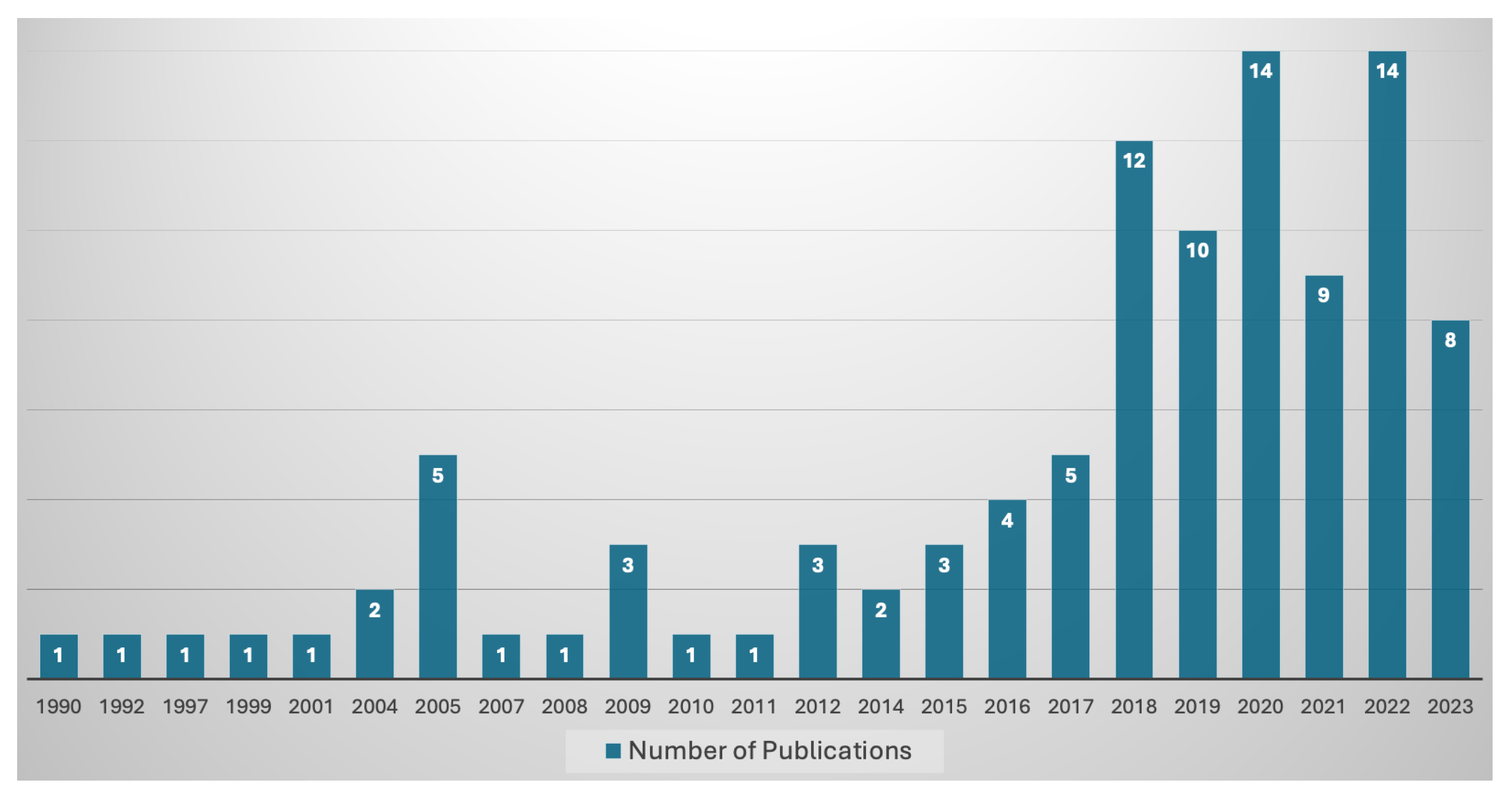
Articles published between 1990 and 2023Non-English articles
Table 3. Summary of features/parameters for ELF or EGF.
Weather Data (Historical or Future)Time Features—SeasonalityMiscellaneous or KPIsSensorsHistorical Target
Solar radiationHour of dayEnergy priceInside temperatureElectricity load
Outside temperatureDay of the weekReheat coefficientDoor opened/closedWind turbine velocity
Wind speedMinute of hourCOVID-19HumidityHeating load
Relative HumidityDay of monthHolidaysOccupancyCooling load
Cloud coverMonth of yearBuilding details-Solar energy
Wind directionYearUsers’ behaviour--
Table 7. Summary of DL regression models for EF.
ReferencesModel/MethodApplicationsFindings
 [102]FFNNGeneral EF applicationsDescribed as a basic NN with input, hidden, and output layers, suitable for various EF applications.
 [103]RNNsSequential data analysisHighlighted for their ability to efficiently handle sequential data, making them ideal for time-series forecasting in energy.
 [104]LSTMVSTLF, STLF, MTLF, LTLFNoted for their capability to learn long-term dependencies, which is crucial for accurate EF over different horizons.
 [72]GRUVarious EF applicationsFound to perform better on smaller datasets, offering an efficient alternative to LSTM with fewer parameters.
 [106]CNNStructured grid-like dataSpecially developed for handling structured grid-like data, providing significant advancements in EF applications.
 [103]Bidirectional RNNsSequential data analysisSuitable for various EF applications due to bidirectional processing for enhanced temporal dynamics understanding.
 [108]DBNStructured grid-like dataSuitable for various EF applications, emphasising deep, hierarchical feature extraction from structured data.
 [109]RRBFNStructured grid-like dataRRBFN outperforms other EF models.
Table 8. Summary of ensemble methods for EF.
ReferencesModel/MethodApplicationsFindings
 [110]Ensemble learningGeneralIntroduced the concept of using multiple models for a single procedure to reduce prediction error.
 [111]BEM and GEMNN domainShowed that prediction error can be reduced using BEM; GEM helps guard against overfitting.
 [116]NN learners train on TBM outputELFUtilised for one-step-ahead ELF, showcasing ensemble models’ adaptability.
 [21,117,118]ZI RegressionEGFApplied to datasets with a high number of zero values, employing a two-step process for regression results.
 [112,113]Stacking and votingGeneral ML applicationsEmployed weights for each model to optimise predictions, aiming to reduce bias and variance.
 [114]Bagging and boostingGeneral ML applicationsFocused on reducing bias and variance, fundamental strategies in ensemble learning.
 [115]Optimisation-based nesting strategyProduce basic learnersOptimised ensemble weights and hyperparameters for regression problems.
Disclaimer/Publisher’s Note: The statements, opinions and data contained in all publications are solely those of the individual author(s) and contributor(s) and not of MDPI and/or the editor(s). MDPI and/or the editor(s) disclaim responsibility for any injury to people or property resulting from any ideas, methods, instructions or products referred to in the content.

