Article

Predictive Control of a Real Residential Heating System with Short-Term Solar Power Forecast

1
Institut für Nachhaltige Energiesysteme, Hochschule Offenburg, 77652 Offenburg, Germany
2
Fraunhofer Institut für Solare Energiesysteme ISE, 79110 Freiburg, Germany
3
P3R GmbH, 89077 Ulm, Germany
*
Author to whom correspondence should be addressed.
Energies 2023, 16(19), 6980; https://doi.org/10.3390/en16196980
Submission received: 31 July 2023 / Revised: 26 September 2023 / Accepted: 29 September 2023 / Published: 7 October 2023
(This article belongs to the Special Issue Artificial Intelligence in Energy Efficient Buildings)

Abstract

:
Predictive control has great potential in the home energy management domain. However, such controls need reliable predictions of the system dynamics as well as energy consumption and generation, and the actual implementation in the real system is associated with many challenges. This paper presents the implementation of predictive controls for a heat pump with thermal storage in a real single-family house with a photovoltaic rooftop system. The predictive controls make use of a novel cloud camera-based short-term solar energy prediction and an intraday prediction system that includes additional data sources. In addition, machine learning methods were used to model the dynamics of the heating system and predict loads using extensive measured data. The results of the real and simulated operation will be presented.

1. Introduction

In 2021, almost half of the global energy demand for buildings was used for space and water heating. More than 60% of the heating energy demand is met by fossil fuels and accounts for 7% of the world-wide energy-related CO 2 emissions [1]. Heat pumps (HPs), especially in combination with rooftop photovoltaic (PV) systems, will play an essential role in decarbonizing this sector. According to a scenario by the International Energy Agency, the number of heat pumps worldwide will reach 600 million in 2030, more than triple compared with that in 2020 [2].
Heat pumps offer electric demand-side flexibility, especially in combination with thermal storage and other heating options. Therefore, classic consumers are increasingly becoming prosumers with complex energy systems that offer many opportunities for optimization. Accordingly, efficient home energy management systems (HEMSs) grow in importance since they help prosumers balance local renewable generation and consumption, increase self-consumption, reduce energy costs, and increase the security of the supply. As an interface to the smart grid, HEMSs can support the operation of a higher-level power grid and help it use its resources efficiently [3].
In the literature, a variety of different system architectures and control methods are proposed to achieve the different energy management goals, ranging from simple rule-based controls to generic algorithms, swarm optimization, and model predictive controls [4,5]. HEMSs with basic rule-based controllers might, for example, attempt to maximize the self-consumption of photovoltaic power by feeding excess photovoltaic power into the battery during the day until it is full or drawing power from the battery at night until it is empty. Such approaches are robust and work well for simple settings, but are less suitable for more complex optimization tasks. Predictive controls, which may use predictions of local consumption, generation, and other influencing parameters, as well as models of system dynamics, can significantly improve the performance of such energy management systems compared with conventional controls, as was shown for model predictive control (MPC) in [6]. However, the actual implementation in a real system presents several challenges, including providing real-time predictions of loads and generating and modeling the system components, so case studies in the literature are still quite limited [7].
This paper presents such a case study on the development and demonstration of an advanced predictive HEMS for a real two-family house with a PV system and a complex heating system including a heat pump and thermal storage. Two predictive control methods will be presented, a simple heuristic control and a more sophisticated MPC approach employing machine learning tools. In both methods, the control objective is the increase in the self-consumption of PV power. The particular novelty is that the HEMS makes use of a cloud camera-based short-term forecast for the PV power, which is described in detail in [8].
PV power can fluctuate on very small timescales due to passing clouds which shade the PV system. Forecasting these fluctuations for the next minutes or hours is not trivial and always contains a certain degree of uncertainty, which has to be considered in energy management systems. Forecasts of solar irradiance and PV power can be retrieved from different data sources, depending which time horizon and resolution is required [9]. Only few studies use real PV power forecasts with uncertainties for HEMS applications. Mostly, these use PV power forecasts based on recent measurements or Numerical Weather Predictions (NWPs) provided by weather services [10,11]. However, these forecasts are not suited to predict the timing of irradiance ramps on a minute time scale. For controlling a heat pump, it is beneficial to have accurate forecasts of these fluctuations, since the heat pump has a minimum run time of several minutes. We use, therefore, an innovative forecasting approach based on all-sky imagers (ASI), taking pictures from the sky every 10 s. They can provide forecasts with a very high resolution for a time horizon of up to 15 min, resolving the movement of single clouds. To cover longer forecast horizons of up to 24 h, we calculate a second forecast based on a combination of satellite-based forecasts, the persistence of recent measurements, and NWPs with a resolution of 15 min. This forecast has a resolution of 15 min. Satellite-based forecasts have a higher spatial and temporal resolution than NWP-based forecasts and a better forecasting performance for horizons of several hours into the future [12].
Increasing PV self-consumption in power-to-heat systems is a worthwhile goal, as it helps both the system operator and the grid operator through saved electricity costs and reduced load on the power grid. One can find numerous approaches in the literature. The use of storage for electrical and thermal load management is discussed in [13], demand side management strategies can be found in [14], and the appropriate sizing of PV systems and storage is explored in [15]. Energy management strategies based on predictive algorithms are discussed in [16]. Predictive algorithms have been shown to improve the self-consumption of PV-controlled systems and reduce operating costs [17].
Several research projects have already been carried out in the field of predictive energy management of heat pumps in buildings. These often focus on reducing the operational cost of house heating and electricity consumption to achieve economical savings [18,19] or on improving energy efficiency and optimizing the performance of the heating systems [20,21]. Weeratunge et al. implemented a mixed integer linear programming-based model predictive controller on a solar assisted ground source heat pump and compared the usage of thermal storage in the system, achieving 7.8% of savings and peak shaving [22]. Kajgaard et al. estimated the savings with a linear-programming-based model predictive control for a domestic heat pump by shifting the loads based on the electricity spot price, achieving savings between 7% and 12% [23].
Whereas many works in this field are based on classical strategies of predictive control with physical models, recent publications use machine-learning (ML)-based models for the optimization of these systems [24,25,26]. The usage of artificial neural networks (ANNs) with Long Short-Term Memory (LSTM) architectures [27] can be useful for the modeling and prediction of dynamical nonlinear systems [28,29]. Also, the use of ML techniques for the forecasting of loads has been intensively studied [30,31,32].
The rest of the paper is structured as follows. In Section 2, we present the real inhabited Projekthaus Ulm, including its technical equipment, which in this paper serves as a test environment for the implementation of the new control strategies and prediction algorithms. Then, we describe the methodology on which the short-time forecast used is based, namely the use of sky images for the shortest time scales and the combination with satellite data and numerical weather forecasts for longer time scales. In addition, we describe how these forecasts can be used for simple heuristic control to achieve an increase in PV self-consumption. Then, we present a more complex model-based optimizing control that uses machine learning methods to predict the system dynamics. In Section 3, the results of the PV short-term prediction, the heuristic control, and the model-based control from the real case study are presented and discussed, before a summary follows in Section 4.

2. Materials and Methods

2.1. Residential Building ‘Projekthaus Ulm’ as Real Demonstration Environment

The Projekthaus Ulm (PHU) is a low-energy house inhabited by a family of four. The house is equipped with a 9 kWp and a 4 kWp PV system and a 4 kWh battery storage. The core of the heating system consists of a 14 kW air-to-water heat pump and an 800 L thermal stratified storage tank with a max. 6 kW heating rod. Bivalent operation is made possible by a supplementary pellet burner, which is used primarily during periods of low outdoor temperatures when the efficiency of the heat pump drops [33]. The system allows for heating via underfloor heating and conventional radiators, as well as hot water delivery via a freshwater station. Due to the fact that the heat storage reaches a temperature of over 60 °C during operation, the requirements according to DVGW worksheet W 551 in combination with the German Drinking Water Ordinance are fulfilled, and as the usable hot water is not delivered directly from the thermal storage, further disinfection is not included in the modeling and analysis. A schematic of the installed heating and electric system is shown in Figure 1.
The installed heat pump uses the technology of direct condensation, where an immersed heat exchanger coil in the storage tank acts as the condenser and realizes the heat transfer, increasing the water temperature. The heat transfer efficiency increases with this configuration, as no additional pump is required between the condenser and the storage tank, decreasing energy losses [35]. However, since the energy transfer is via the refrigerant and the energy transfer from the coil to the fluid has to be considered, the physical modeling is more complex than that for conventional heat pumps [36,37].
The PHU is equipped with extensive measurement technology that measures numerous thermal and electrical generators and consumers with high temporal resolution. State variables such as room temperatures and outdoor temperatures are also recorded and collected in a database [34].
One goal that is being investigated and pursued in the PHU and also in this work is to increase the PV self-consumption share ( S C S ). This is defined as
S C S = E PV , c E PV , g ,
where E PV , g is the PV energy generated over the study period and E PV , c is the PV energy consumed from it directly or after intermediate storage in a battery in the house [38]. Since this work is about using the flexibility of the heat pump and thermal storage, the battery was intentionally not used.
A special feature of the PHU is an already installed rule-based or heuristic control of the heat pump, which aims to increase the PV self-consumption. For this purpose, a controller observes the current measured values of the PV power and the thermal tank temperatures. If certain conditions are satisfied (average tank temperature below 40 °C, PV power values above the threshold of 1.5 kW during the last 10 min, current PV power at least 3.5 kW), the heat pump is started to charge the thermal storage tank to the maximum. This behavior is called single charging in the following. This is based on the assumption that PV generation will continue to be above the threshold value during the subsequent period of storage charging. Thus, ultimately, a persistence prediction of the PV power is already used.
In this work, we aim to further improve the existing heuristic control of heat pump with persistence prediction. For this purpose, we investigated two different predictive control approaches. The first approach extends the existing heuristic control. The second approach uses the more complex model predictive control, using dynamic models of the heating system. Both approaches notably use innovative local predictions of PV generation, which are described below.

2.2. Short-Term PV Power Forecasting

Within the project, two forecasting approaches were used as inputs to the energy management systems. The first is an ASI-based nowcasting system that uses data from a sky camera and real-time irradiance measurements. It has a maximal forecast horizon of 15 min, depending on the cloud situation, and a resolution of 10 s. The second is an intraday forecasting system that combines satellite data with data from numerical weather prediction (NWP) models and real-time irradiance measurements. It has a maximum forecast horizon of 24 h and a resolution of 15 min.
The output of both forecasting systems is a forecast of global horizontal irradiance (GHI), which is used as input to a PV simulation to generate a PV power forecast for the two rooftop PV systems at the Projekthaus Ulm using the model described in [39].

2.2.1. ASI-Based Nowcasting System

In the ASI-based nowcasting system, irradiance forecasts are calculated in a step-by-step physically based approach. A detailed description of the nowcasting system can be found in [8,34]. A fisheye camera takes pictures of the whole sky every 10 s. The first step of the forecasting algorithm is calculating a cloud mask using the image pixel values as inputs. Every pixel is classified as cloud or clear sky. The cloud movement is then calculated using an optical flow algorithm. The resulting motion field is applied in the next step to the cloud mask using inverse mapping to retrieve a forecasted cloud mask. From the forecasted cloud mask, a binary time series of shadow is extracted for the pixel of the sun position in the image, which is the position that shades the camera. This time series of shadow and recent irradiance measurements are used as input for a statistical model that calculates an irradiance forecast. Figure 2 illustrates the main steps from images of the sky to an irradiance forecast.
To fill gaps and to provide forecasts for all times of the day, additionally, a persistence forecast based on real-time irradiance measurements is calculated. Gaps in the ASI forecasts occur since they can only be calculated for zenith angles smaller than 80°. Also, if the clouds move fast or cloud height is low, it can happen that a forecast run ends before the 15 min horizon because the visible clouds were shifted out of the image. We use the persistence of the clear sky index ( k * ), which is defined as k * = GHI / GHI clear , to account for the diurnal cycle. GHI clear is the clear sky irradiance, which we calculate using the method described in [40]. The persistence forecast is then calculated from Equation (2), where t is the forecast valid time and t 0 is the start time of the forecast,
GHI pers ( t ) = GHI clear ( t ) · k * ( t 0 ) .
For the implementation of the ASI-based nowcasting system at the Projekthaus, a camera (FE9381 from Vivotek, Taipei, Taiwan) and a pyranometer (MS-80 from EKO, Lagos, Nigeria) were installed on the roof. The data are transferred in real time to a computer in the Projekthaus that processes the data.

2.2.2. Intraday Forecasting System

The ASI-based nowcasting system forecast alone does not have a large enough prediction horizon that aligns optimally with the requirements of the model predictive control approach. Recognizing this, a solution that merges different forecast sources was implemented.
The intraday forecasting system combines irradiance forecasts from several different sources via a machine learning model to generate an optimized forecast for each intraday forecast horizon, ranging from 15 min up to 24 h. Three different irradiance forecasts are used as input for the combination model: a persistence forecast generated from irradiance measurements as described in Equation (2), an NWP model forecast from the ECMWF (European Centre for Medium-Range Weather Forecasts) Integrated Forecasting System, and a forecast generated from cloud motion vectors on satellite images [41]. The input forecasts are combined through a linear regression model, which essentially conducts a weighting of the different input forecast types depending on the forecast horizon. The model was trained on a historic data set with a time span of 5 months (May–September 2019).

2.3. Predictive Heuristic Control Approach

The first control approach presented here aims to improve the already implemented heuristic control for single charging of the storage (cf. Section 2.1). The persistence prediction used so far has the disadvantage that it cannot predict imminent PV power dips due to clouds. If a drop in PV power actually occurs, power must be drawn from the grid or the single charge must be aborted. Neither of these is desirable. In particular, a certain minimum runtime of the heat pump should not be undercut.
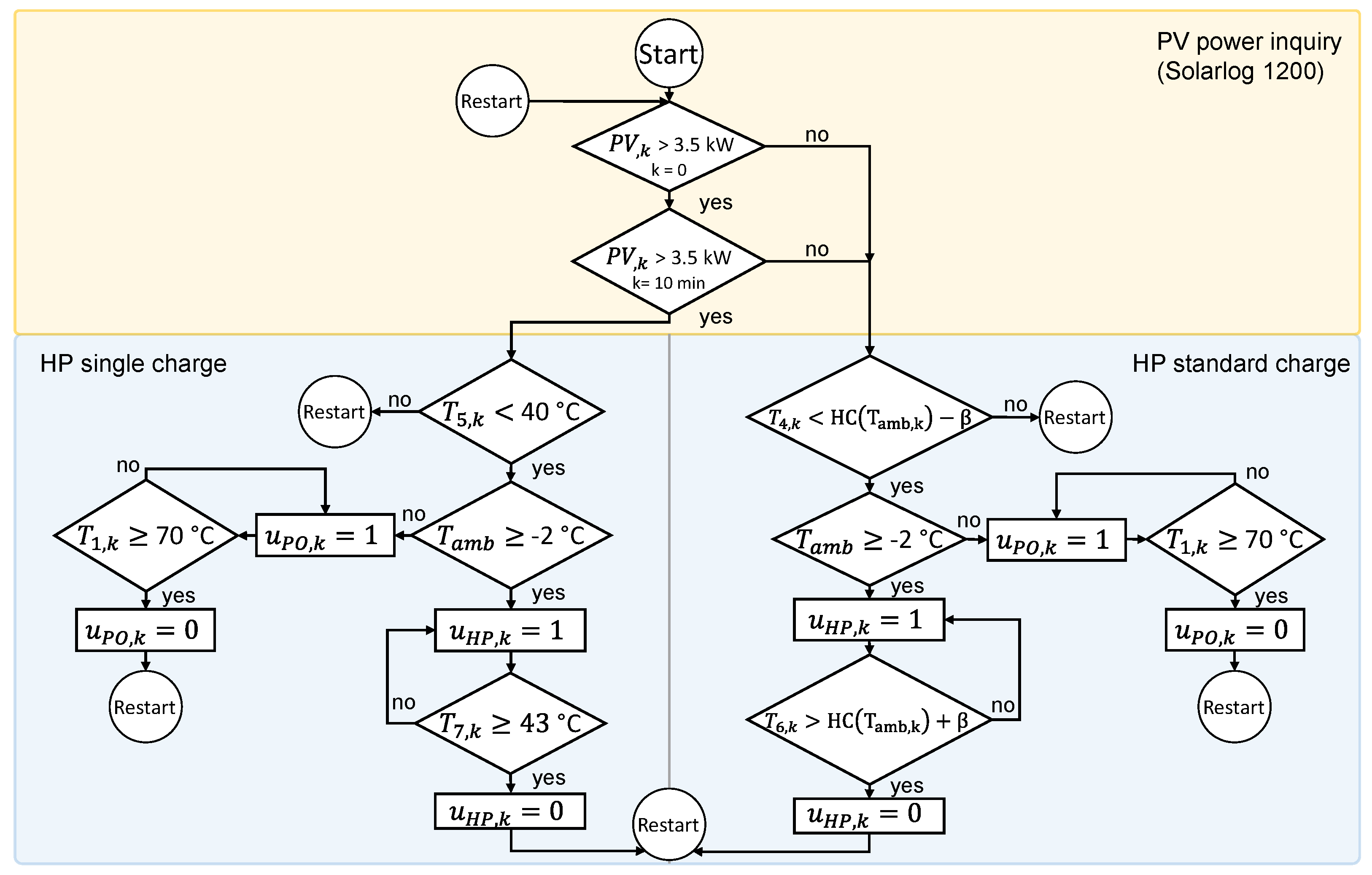
Therefore, persistence prediction is replaced by cloud camera-based PV prediction, as presented in Section 2.2.1. The existing heuristic controller was adapted to trigger a one-time charge when the current power is above a threshold of 3.5 kW and the ASI-based prediction predicts that this power will be maintained over the following 10 min, see Figure 3.
Data exchange with the different systems in the Projekthaus Ulm was realized via different protocols like KNX and Modbus. An InfluxDB database was used for storing the data. Controllers and data exchange were implemented based on several Python scripts running as cron jobs on a LINUX system on an industrial PC.
A special challenge in the implementation of the original and also the here-presented improved heuristic controller is that the heat pump has a controller that controls the internal components, like compressor, valves, pumps, etc. This internal controller does not initially allow the desired single charge. Therefore, the control implemented in the heat pump, which is based on a predetermined heating curve and dead zone controls (hysteresis), must be “tricked” by the predictive controller by appropriately faking appropriate temperature input data, which results in the heat pump turning on and off and allows for a single charge.

2.4. Predictive Model-Based Control Approach

2.4.1. Model Predictive Control with Hybrid System Model

The second control method based on MPC presented here differs fundamentally from the rule-based heuristic approaches discussed previously.
In MPC, mathematical optimization algorithms are used to calculate optimal schedules for certain manipulated variables—in our case, the activation of the heat pump—over a certain time horizon [42]. This is performed by solving a mathematical optimization problem in which an objective function is minimized or maximized. In doing so, the algorithm is able to ensure compliance with defined state and control limits, such as limit temperatures of the thermal storage or minimum runtimes of the heat pump. The optimization also includes predictions of the controlled system’s behavior. This is performed, on the one hand, on the basis of a dynamic model of the system behavior, and, on the other hand, on the basis of predictions of relevant external influencing parameters, like PV power or thermal loads in our case. The MPC approach can reach its potential in the home energy management sector if the forecast horizon covers at least one daily cycle. Accordingly, the intraday forecast described in Section 2.2.2 is needed here instead of the short-term forecast from Section 2.2.1. In addition, the MPC can handle disturbances and model errors by updating the optimization calculations in regular time steps, taking into account current measurements of the initial states as well as updated predictions of external time-varying parameters. Only the first steps of the control schedule are actually realized until an updated timetable is available again. Thus, one works with a receding prediction horizon [17,43,44].
In the following, we will introduce the optimization problem in a little more detail. The optimization objective is to maximize the self-consumption of PV power. This can also be interpreted as minimizing the grid power consumption P gc , k . We therefore choose the cost function J to be minimized as
J ( u HP , u PO ) = k = 0 N P gc , k 2 .
Here, k denotes the index of the time step t k within an equidistant discretization [ t 0 , t 1 , , t N ] of the prediction time horizon. For each new optimization, t 0 then corresponds to the current real time and, thus, to the starting point of the new optimized schedule. The heat pump in our specific case continued to operate automatically with the standard operation and the scheduling and control were performed with the single charge mode. To include this into the optimization, the different modes were formulated as two separate heat pumps. The vector u H P = ( u HP , 0 , u HP , 1 , , u HP , N ) T is a vector of binary control variables u HP , k { 0 , 1 } that denote the switching state of the heat pump in the standard operation. The vector u H P S C was defined similarly to represent the heat pump in the single charge operation. The vector of binary variables u PO for the pellet oven switching state is defined accordingly. u H P , u H P S C , and u PO , together, thus represent the control schedule.
The quadratic cost function penalizes high P gc , k values particularly strongly, and thus avoids load peaks, which is desirable from the grid operator’s point of view on the one hand and can also bring economic advantages for plant operators with certain electricity contracts. The minimization of the cost function (3) is now performed by means of special mathematical optimization algorithms, taking into account a number of constraints, which are presented below in the form of equations and inequalities (4) to (11).
In particular, the consumed grid power P gc = ( P gc , 1 , , P gc , N ) T over the prediction horizon is related to the control schedules u HP and u PO by the the electrical power balance,
P gc , k + P PV , k = P HP , k + P H P S C , k + P PO , k + P load , k + P gf , k , for every k { 1 , , N } .
Next to P gc , k , we have P PV , k as the generated PV power on the generation side, whereas on the load side, P HP , k , P H P S C , k , P PO , k , and P load , k denote the power consumed by the heat pump in the standard operation, the heat pump in the single charge operation, the pellet oven, and the other electrical loads in the house, respectively, and P gf , k is the power fed into the grid. We recall that the battery is not considered here.
Here, the generated PV power P PV , k and the power consumed by other electrical loads P load , k are external time-varying parameters and have to be provided via forecasts. The power consumption of each of the formulated heat pumps P HP , k and P H P S C , k are related to their control variables, i.e., the switching states u HP , k and u H P S C , k , respectively, by means of a regression model that has T amb , k , the switching states u HP , k and u H P S C , k , and the temperature T 8 , k at the bottom layer of the stratified tank as inputs. The power consumption of the pellet oven P PO , k is related to the control variable, i.e., the switching state u PO , k , by means of the simple relation P PO , k = u PO , k · P PO , nom with a constant nominal pellet oven power P PO , nom . Note that the values of P gc , k 0 and P gf , k 0 then follow from the other values due to (4).
Another constraint that has to be taken into account during optimization is the dynamics of the heating system, consisting of heat pump, pellet oven, thermal storage, and thermal loads, which are modeled by
x k + 1 = f ( x k , c k , u HP , k , u PO , k ) ,
x 0 = x i c .
Here, the dynamic state vector x k = ( T 1 , k , , T 8 , k ) T contains the temperature levels of different positions in the thermal stratified storage. x i c is the vector of initial temperatures at time t 0 , coming from current measurements. The vector c k = ( T room , k , T amb , k , Q ˙ UF , k , Q ˙ Rad , k , P FW , k ) T contains the external parameters that influence the heating system. Here, T room , k is the temperature of the room where the heat pump is installed. T amb , k is the outside ambient temperature, which is especially important for the efficiency of the heat pump. Q ˙ UF , k and Q ˙ UF , k denote the heat flows of the underfloor heating and the radiators to the heated rooms, respectively. P FW , k is the electrical power of the fresh water pump, which influences the temperatures in the thermal storage by extracting heat for hot water.
In modeling the heating system, no physical equations were used or the parameters of classical system models identified, so no explicit expressions for the function f are available. Instead, a hybrid model was used here that combines a neural network for the dynamics of the stratified storage tank and direct condensation with a regression model for the heat flow of the heat pump. The reason for this data-based approach was that the authors could not achieve sufficient model quality with the classical modeling approaches, probably due to the particular complexity of the combination of direct condensation and stratified storage.
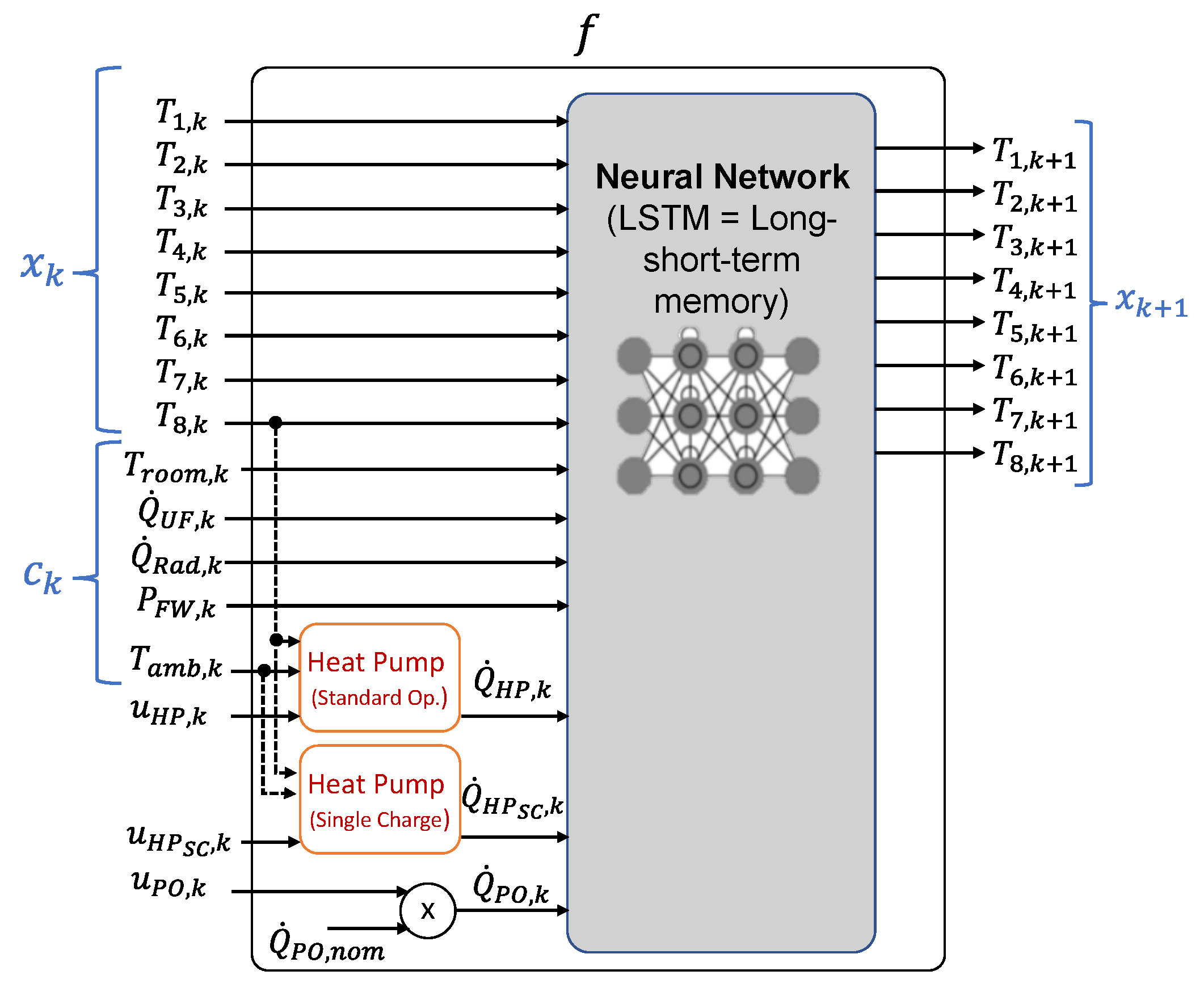
Neural networks of the type Long Short-Term memory (LSTM) were used for modeling the stratified storage, see Figure 4. The LSTM approach is especially suited for the modeling of system dynamics [45]. The network was trained on the basis of measurement data from the Projekthaus Ulm in such a way that the new system states x k + 1 can be predicted with the aid of the input data, consisting of the system states x k , the external parameters c k , and the controls u HP , k , u H P S C , k , and u PO , k from the old time step k. Note that the model uses internal auxiliary variables, namely Q ˙ HP , k , Q ˙ H P S C , k , and Q ˙ PO , k , which are the heat flows of the heat pump and the pellet oven and which depend in particular on the control parameters u HP , k , u H P S C , k , and u PO , k as well as on external parameters. For additional details, we refer to [7].
The regression model of the heat pump was first fitted to the data provided by manufacturer’s capacity tables, and then fine-tuned and validated with measured data from the Projekthaus Ulm. The inputs for this regression model were the outside ambient temperature T amb , k , the switching state of any mode of operation of the heat pump, u HP , k or u H P S C , k , and the temperature T 8 , k at the bottom layer of the stratified tank. This creates a feedback within the hybrid model that takes into account the thermal stratification of the tank and the environment conditions and uses this information to describe the heat flow of the system. This approach is based on the work of Sawant [46].
In addition to (4) and (5), an optimal solution must satisfy further constraints, such as
x min x k x max
u HP , k · T 7 , k R L max
u H P S C , k · T 7 , k R L max
H C ( T amb , k ) + β lower u HP , k · T 4 , k H C ( T amb , k ) + β upper
0 u HP , k + u H P S C , k + u PO , k + 1
All relationships above should apply to all k { 0 , , N } , respectively. The authors of (7) describe lower and upper limits for the temperatures in the different thermal storage layers. The authors of (8) and (9) allow the operation of the heat pump in any mode only if the maximum return line temperature is below R L m a x (in the experiments, equal to 43 °C). The authors of (10) include the behavior of the heat pump for the standard operation into the optimization problem, where it should start automatically if a certain temperature in the middle of the heat tank leaves a certain temperature range that is defined on the basis of a heating curve H C and lower and upper offset values β lower and β upper . The authors of (11) prohibit the heat pump to operate in both modes simultaneously and also prohibit the pellet oven and heat pump running in any operation mode at the same time; this last condition was a wish of the home owners.

2.4.2. Practical Implementation of the Controls

The practical implementation of an MPC is associated with some challenges. For example, the repeated solution of the optimization problem at each time step requires short computation times, which can lead to high hardware requirements for complex optimization problems. In power system optimization, it is often challenging to provide predictions of the influencing factors, which depend on weather or human factors and often have some stochastic components.
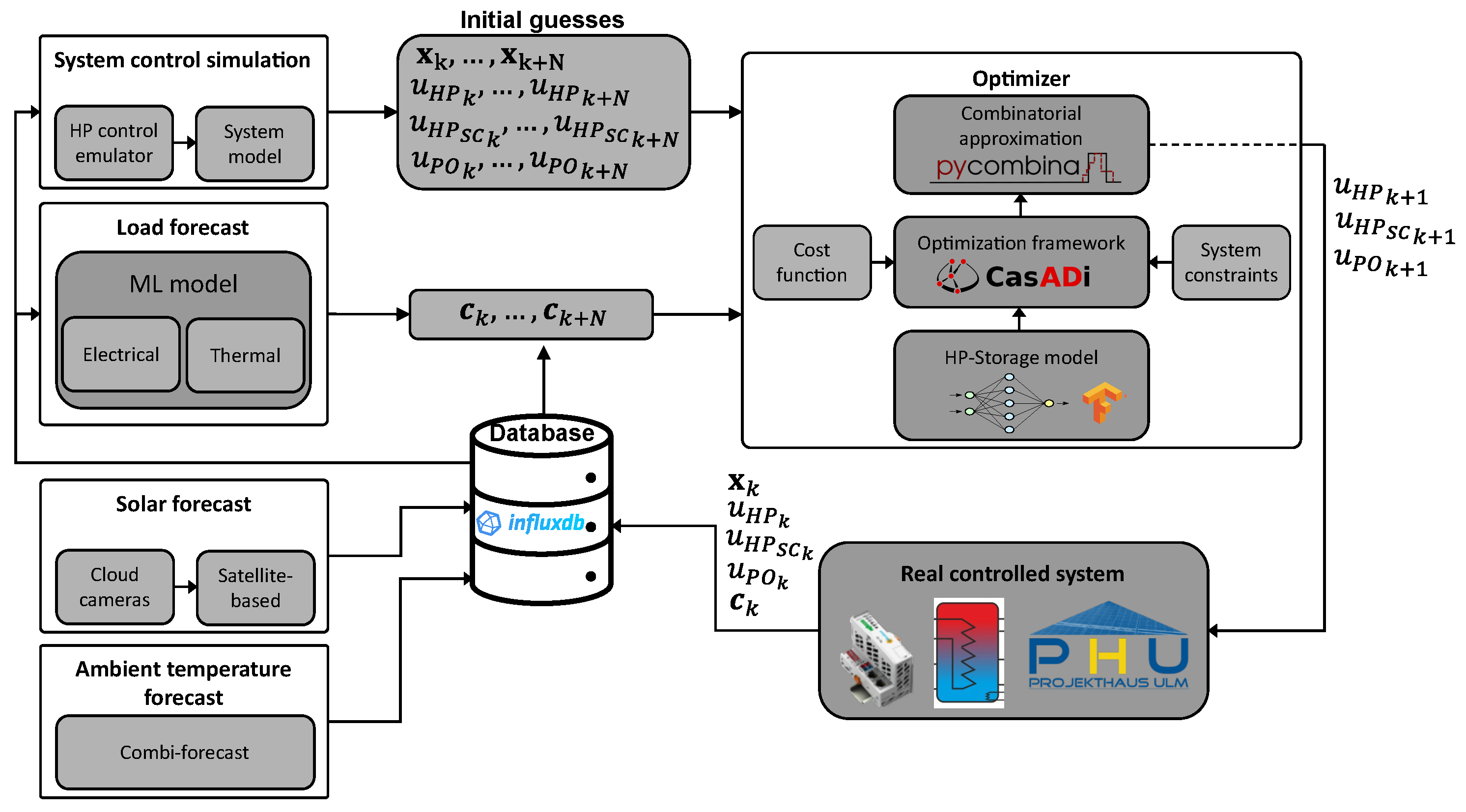
Therefore, in our case study, an innovative cloud camera-based combined forecast was used for PV forecasting. Machine-learning-based solutions were used to forecast the electrical and thermal loads. A challenge was often also the clean acquisition of data during operation. In the case study, for example, we had to work with electrical signals from the fresh water pump contaminated by electric couplings, which first had to be cleaned up using machine learning methods before they could be used. For details, refer to [7]. Figure 5 shows the architecture of the practical implementation of the control system in the Projekthaus Ulm.
Python Keras was chosen as the framework for LSTM development because it has an extensible and modular focus that can be used for rapid deep neural network experiments [47]. The optimizer was also implemented in Python. Due to the binary variables and the underlying non-linearity of the LSTM model trained with a nonlinear activation function, the underlying optimization problem belongs to the class of Mixed Integer Nonlinear Problems (MINLP). For its solution, we used in a first step the algorithmic differentiation framework CasADi [48] together with the nonlinear solver IPopt [49] to obtain a relaxed continuous solution. Afterwards, we used a combinatorial approximation approach for the calculation of the integer states with the binary approximation library pycombina [50].

3. Results from Projekhaus Ulm

3.1. Results for PV Power Forecasting

3.1.1. ASI-Based Nowcasting System

We present the results of the ASI-based forecasts of GHI and PV power from the Projekthaus for a data set containing May and June 2019. Figure 6 shows the relative Root Mean Square Error (RMSE) of the GHI and the PV power forecast. The RMSE is calculated from the forecasts p i and the corresponding measurement m i ,
RMSE = i = 0 N ( p i m i ) 2 N .
The relative RMSE is calculated by dividing the RMSE by the average irradiance or power. With the increasing forecast horizon, the relative RMSE increases for all forecasts as expected. The PV power forecast (red) has a slightly higher relative RMSE than the GHI forecast (blue) due to the uncertainty added with the additional computation step. The GHI and PV persistence forecasts are shown in light blue/light red for comparison. They show higher RMSE values than the ASI forecasts for all forecast horizons, with an increasing gap as the forecast horizon increases. This confirms the value of the ASI forecast compared with the persistence forecast currently used in the heuristic control in the PHU.
In addition to the standard error metrics, we developed a specific score adapted for the application of controlling the heat pump. The aim was to control the heat pump in the PHU in a way that the demand is covered by the PV production. The most problematic forecast error that can occur for this application is when the forecast predicts PV production to be higher than the heat pump demand during the heat pump’s minimum run time, but the PV production is actually lower for part of the time. To quantify this error, we look for predicted and measured events where the heat pump can operate with the power (p) generated by the PV system for at least a time interval Δ t . For simplicity, Δ t always starts at the beginning of the forecast,
E v e n t f c : i f p f c ( Δ t f c ) > p t h r e s s h o l d ,
E v e n t m e a s : i f p m e a s ( Δ t m e a s ) > p t h r e s s h o l d .
The minimum run time of the heat pump of 7 min is used as Δ t and the threshold for power generation ( p t h r e s s h o l d ) is 3.5 kW.
In total, 9410 forecasts were validated using the data set May–June 2019. There were 2236 measured events detected and 2959 forecasted events. Of the measured events, 97.5% were forecasted correctly (hitrate), and of the forecasted events, 73.7% were also measured (precision). The precision is the most relevant score here, since it gives the probability of a forecasted event to actually happen. For comparison, we again validate the persistence forecast. Here, the hitrate is 97.7% and the precision is 69%.
To make the forecasts more reliable, we want to identify forecasted events that occur with a higher probability. Therefore, we change Δ t f c to 15 min, since the timing of the forecasted ramps can be wrong. Table 1 shows the result. The number of forecasted events and the hitrate are slightly reduced for Δ t f c = 15 min. However, the precision increases to 78.0%. This information could be used to improve the performance of the energy management systems.

3.1.2. Intraday Forecasting System

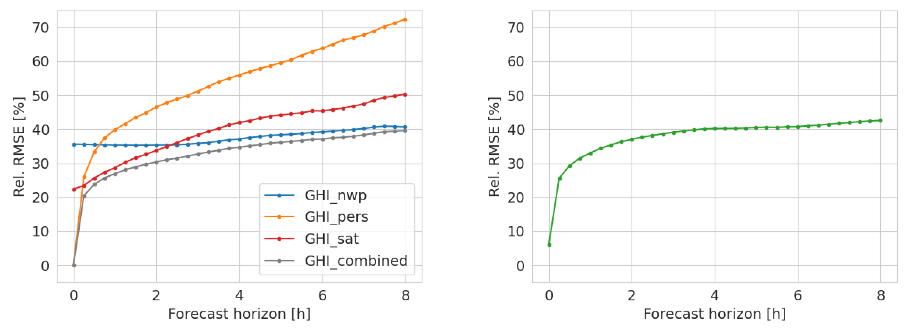
For evaluation of intraday forecasting, we show results for a period from May to August 2019. The left panel of Figure 7 shows a comparison of the performance in terms of RMSE for the different input irradiance forecasts and the optimized combination forecast depending on the forecast horizon, up to 8 h. The persistence forecast (orange line) performs well for small horizons up to about 15 min, the satellite forecast (red line) performs best for intermediate horizons up to about 2.5 h, and the NWP (blue line) performs best for large horizons of several hours. The performance of the optimized combination forecast obtained from the linear regression model is given in gray. As expected, the combination forecast always exhibits a lower RMSE than any of the individual input forecasts. The performance (also in terms of RMSE) of the PV power forecast, which is obtained after applying a PV simulation to the combination forecast, is shown in the right panel of Figure 7. As for the ASI-based forecast, the intraday PV power forecast also has a slightly higher RMSE than the intraday irradiance forecast due the additional modeling step.

3.2. Results of Predictive Heuristic Control

The predictive heuristic controller was implemented in a series of tests in the cold spring period to determine its performance compared with the actual heuristic controller setup. The tests were conducted in the spring period, as during this time there is increased cloud variability that shows variable PV power generation together with heat demand requirement.
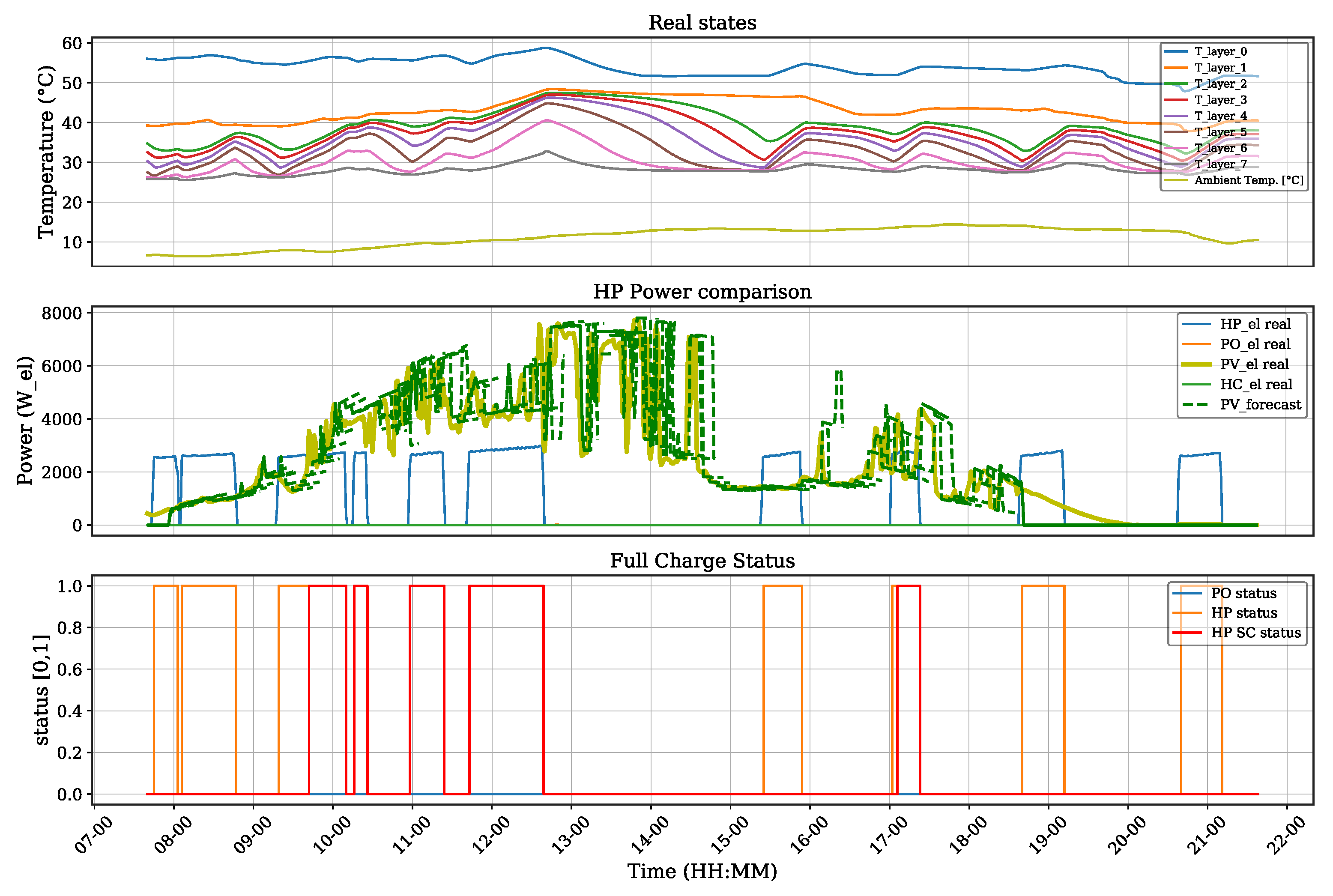
An exemplary test using the predictive algorithm is showcased in Figure 8. The graph shows the layer temperatures in the tank during the test. It also shows the PV power generation during the day, as well as the the different PV short-term predictions at the given time and the HP electrical energy consumption. Lastly, it shows the control actions given by the predictive controller to the system.
The test started in the early morning, when PV power production was low. As the heating curve lower limits of the tank were reached due to the heat requirement, the heat pump controller started a standard heating operation, charging the tank. Later in the morning, another standard charge was performed by the heat pump, as not enough energy coming from the panels was generated. At around 9:40 h. in the morning, the PV power reached the minimum threshold of 3.5 kW and the short-time prediction for that time showed enough power to drive the machine for at least 10 min. The predictive controller started the single charge at this point, allowing the tank to heat for a longer time and to higher temperature limits. The heat pump was turned off after several minutes, as the PV power dropped again under the minimum threshold value and as the last calculated short-time prediction for that time showed a drop in the expected power. This is possibly due to a cloud covering the sky. This single charge operation was followed by a second shorter single charge that lasted for only 10 min, which corresponds to the minimum run time. This short operation occurred as the PV prediction once again showed enough PV power to be produced in the following 10 min, but in this case the real produced PV power dropped again under the set threshold; this was possibly due to a mismatch in the prediction. During the day, further single charge operations were conducted by the predictive controller, allowing the tank to be heated completely through the generated PV energy and the HP. Finally, around 17:00 h. a last single charge operation of the HP was driven. At that time, there was high fluctuation in the PV generation, possibly due to clouds, and as the evening was reached, less power was available. Although the PV power was not enough to completely satisfy the HP electrical demand, the single charge operation was driven during a peak in PV power where heating was also required. This used as much of the remaining PV power as possible for heating.
The results for this test show a calculated self-consumption score of 27.14%. For comparison, a simulation was performed for the same day using the hybrid model and an emulator of the actual heuristic controller based on the persistence prediction. The calculated self-consumption score for the simulation resulted in 24.24%, showing an overall improvement of 2.9% utilizing the predictive heuristic control for that day.
A similar test was also conducted for April 19 with similar weather conditions. The results for the test show a self-consumption score of 39.04%. In comparison, the results of the simulation show a self-consumption score of 37.64%. This results, in this case, in an improvement of 1.4% for the self-consumption.
Using a simulation of the actual heuristic implementation as a baseline for comparison, we can evaluate the effectiveness of the predictive heuristic control approach. The results of the tests in this case show a slight improvement in the self-consumption scores against the simulation, showing the viability of this implementation.

3.3. Results for Predictive Model-Based Control

Similar to the previous experiments, a test was conducted to evaluate the operation of the MPC during variable weather conditions and with the required heat demand of the house.
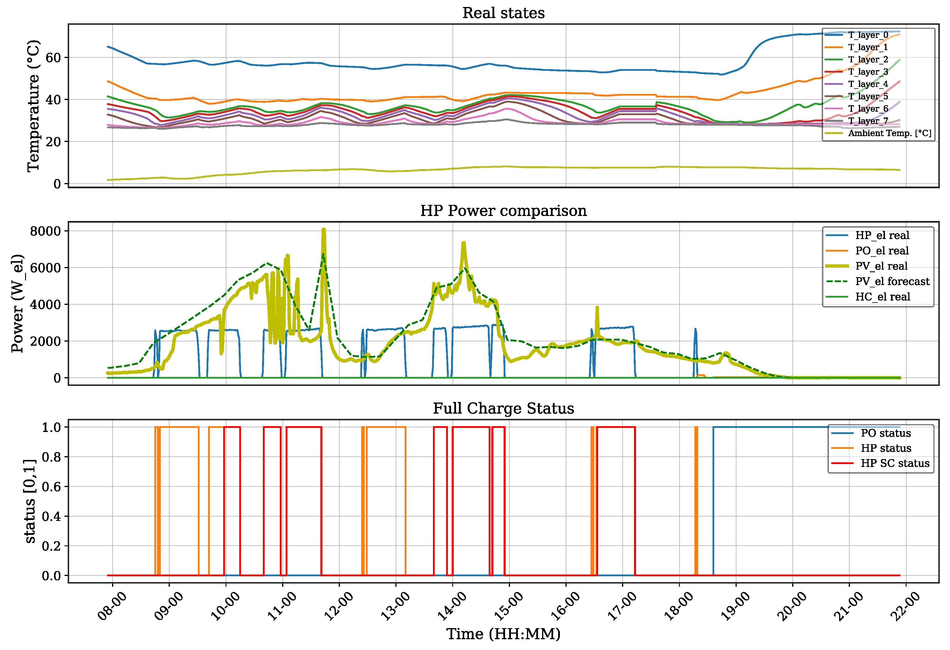
In this test, the model predictive control was driven with a 5 min time interval, and an intraday forecasting system was used for the predictions. The intraday forecast combines weather and solar predictions and provides data with a horizon of a day. The results are shown in Figure 9.
The test started early in the morning, when the storage tank was still warm from a previous charging. As the tank’s lower limits were reached due to high heating demand, a standard heating operation was directed by the still-operating HP standard controller. Later in the morning, as a continuous heating demand was expected, as shown in Figure 10, and as the temperature in the tank was expected to decrease due to the demand, a second standard charge was started, but as the predicted PV power showed that enough power would be available, the MPC decided to start the HP in the single charge operation mode and heat the tank with higher limits. The MPC calculated the optimal states between the heat demand requirement and the PV produced. This can be seen in the following single charge operations conducted by the controller. At around 10.40 h. in the morning, a heating operation was required and the PV power had very high fluctuation. At this time, a single charge was instructed to start charging the tank with as much PV power available, thus delaying a required standard heating operation at around 12:15 h, when a steep drop in the produced PV power can be noted. As the produced power at around 13:40 h was high enough and predicted with a wide power window, the storage tank was heated as much as possible, allowing it to avoid further charging during lower PV power in the early midday and starting a single charge operation during the highest peak of PV power produced that evening.
At around 10:15 h, the single charge operation that was conducted previously by the predictive controller was stopped early. Without this stop, the tank could have been heated further, as no temperature limits were reached and enough PV power was still produced, thus avoiding the operation afterwards (around 10:40 h) where intermittent PV power was produced. This behavior can be attributed to three main factors, i.e., (i) the deviation between the predicted PV power and the real produced power, where no intermittent PV production was expected (as seen in the PV prediction); (ii) the error between the hybrid model and the real behavior of the storage tank, causing a change in the optimizer’s decision during the given control calculation; and (iii) the deviation in the load prediction models, where the optimizer might have calculated a different result for the given schedule with the calculated a expected heating load. However, these deviations show the ability of the predictive controller to respond to changing conditions, where it was able to provide the necessary heat to meet the given demand while maximizing the available PV power even when conditions were not optimal.
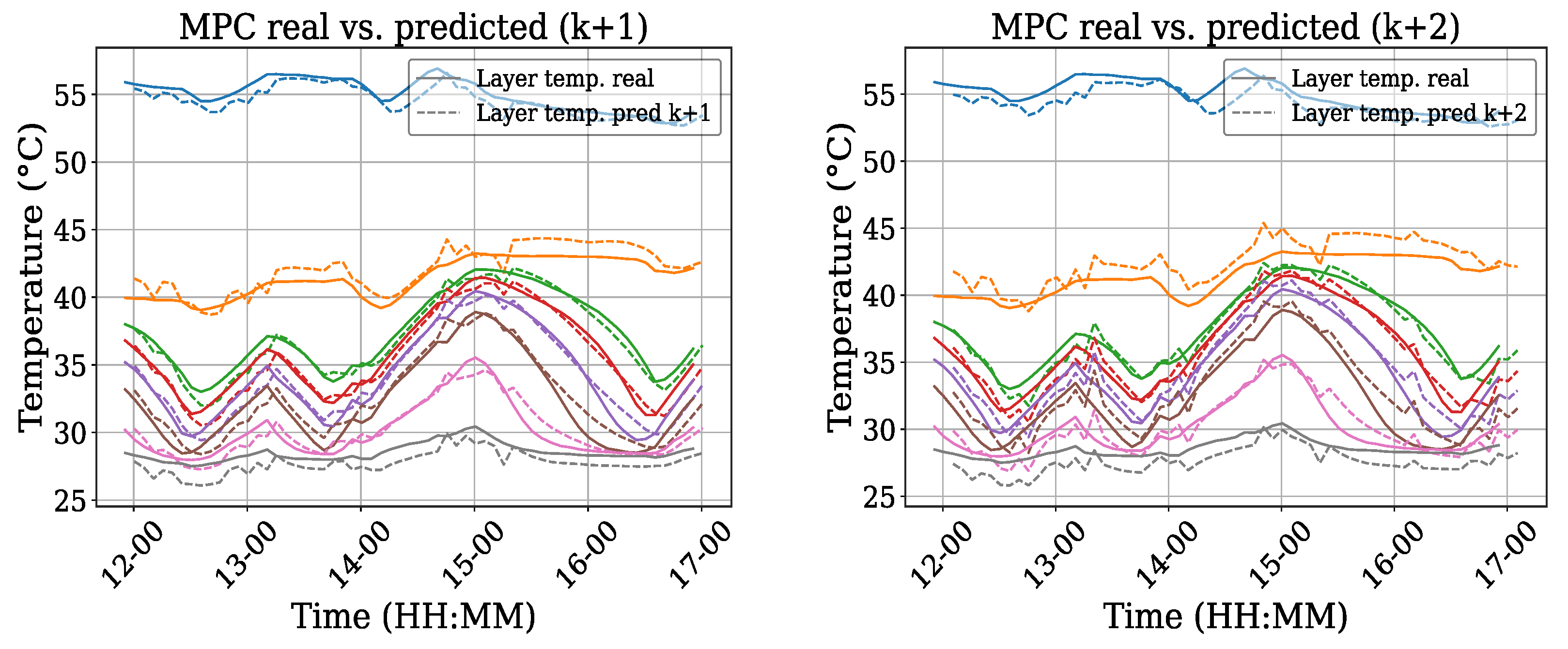
This combination of different models, forecast methods, and input sources proved to work successfully in the test environment. Figure 11 shows the measured system states versus predicted system states during MPC operation with a mean absolute percentage error (MAPE) of 1.68% and 2.60%, respectively, showing, in this case, a good prediction for the predictive controller. The predictions for the thermal loads during the day and the PV power, showed an MAPE of 44.2% and 39.7%, respectively. The difference can be seen in Figure 10. This difference is directly attributed to the models, and the sampling used.
The predictive controller showed promising improvements when compared with a simulation performed with the same conditions but using a classical heuristic control approach. The results show a decrease in the grid energy of 36.03% with a self-consumption of 48.48%.

4. Conclusions

This paper presents the development, implementation, testing, and evaluation of two new predictive control approaches to maximize PV self-consumption for a real occupied residential house with a PV system, a heat pump, and thermal storage. A special feature is the use of a newly developed short-term PV power prediction system based on all-sky imager data and an intraday prediction system that includes additional data sources.
The first predictive control approach presented is rule-based and uses an ASI-based nowcasting system that provides PV power predictions with a high temporal resolution of 10 s over a time horizon of 15 min and is particularly suitable for predicting ramp events. The controller starts the heat pump when this nowcasting system predicts sufficient solar radiation over the minimum run time of the heat pump and the thermal storage tank has sufficient intake capacity to be filled accordingly. As a reference, a comparable controller was considered that makes the decision based only on a persistence prediction, in which past and current irradiance measurement data are assumed to remain constant into the near future.
Test results show that the new ASI-based nowcasting system is superior to the persistence prediction for PV power in terms of RMSE. Also, the new rule-based controller for the heat pump using this improved prediction was able to show a slight improvement in PV self-consumption compared with the reference system in simulation and real test runs.
The second predictive control approach presented is based on the model predictive control method and optimizes a heat pump deployment schedule over the upcoming 24 h. For this purpose, the controller uses a 24 h PV power prediction with 15 min resolution from an intraday forecasting system combining current measured irradiance data, ASI images, satellite images, as well as NWP irradiance forecasts. Test results show that this intraday system also works well and is superior to the persistence forecast in terms of RMSE.
For the design of the model predictive controller, the dynamics of the heating system to be controlled must be modeled numerically. Since the heat pump used works with direct condensation in the storage tank and is therefore difficult to model physically, a neural network of the LSTM type was trained on the basis of extensive measurement data. The corresponding model shows good agreement with validation measurement data, which were not used for training. The MPC-based controller using this model was able to demonstrate its functionality in simulation and test runs, and again a slight improvement in self-consumption was achieved.
In conclusion, both the nowcasting system and the intraday prediction system work in real applications and can be reasonably used for predictive control tasks in a residential building. The 15 min forecast proved to be suitable and useful for the improved heuristic control and the intraday forecast proved to be suitable for the MPC approach. The two predictive control algorithms have also been shown to work in simulations and test runs and can achieve slight improvements in PV self-consumption.
However, the tests and simulations have also shown that the potential for self-consumption improvement in the configuration studied here is quite small. The main causes include the restrictive operating limitations for the heat pump, such as temperature limits and minimum run times, which must be met in addition to meeting the heat demand. Incorporating an additional electric heater into the control system (both rule-based and model predictive) would provide significant additional flexibility here and allow for PV self-consumption to be significantly increased.
There is also further room for improvement with respect to the modeling of the system. A particular challenge was that the existing internal control system of the heat pump continued to be operational, and therefore had to be modeled along with the operational behavior. Here, it would be of great benefit if the internal controllers of future heat pumps had appropriate interoperable interfaces for integration into higher-level energy management tasks.
Future work should focus on a more detailed study of the impact of different forecasting methods and accuracies on the control results, as in this work we focus primarily on demonstrating the foundational capabilities of a predictive control system utilizing local PV forecast methods. Also, further work should accordingly address the integration of a heating rod into the energy management, further improvement of the models, as well as predictions of PV generation and thermal and electrical loads and focus on the interoperability of the different components within increasingly complex domestic energy systems and energy management tasks.

Author Contributions

Conceptualization: A.D., O.V.M., H.R., M.S. and E.L.; Methodology (Forecast): E.L., A.D. and W.H.; Methodology (Controls): O.V.M., R.G. and M.S.; Software: O.V.M., A.D. and W.H.; Testing and Validation: O.V.M., H.R. and A.D.; Writing—Original Draft Preparation: O.V.M. and A.D.; Writing—Review and Editing: O.V.M., R.G. and M.S.; Project Administration and Project Acquisition: M.S. and E.L. All authors have read and agreed to the published version of the manuscript.

Funding

This research was funded by the Ministry of the Environment, Climate Protection and Energy Sector Baden-Württemberg under grant number BWSGD 18001-18002.

Data Availability Statement

The data presented in this study is restricted and partially available on request from the corresponding author. The data utilized in this study is not publicly available due to privacy and data protection considerations. The location where the data was collected is a real inhabited environment, and safeguarding the privacy and confidentiality is of paramount importance. Adherence to ethical guidelines and data protection regulations prevents us from openly sharing this sensitive information. Access to the data will be subject to the guidelines and terms of the Projekthaus Ulm upon request.

Acknowledgments

We thank Patrick Kober from Projekthaus Ulm for his support and the provision of data.

Conflicts of Interest

The authors declare no conflict of interest.

Abbreviations

The following abbreviations are used in this manuscript:
AIArtificial Intelligence;
ANNArtificial Neural Network;
CAGR Compound Annual Growth Rate;
GHIGlobal Horizontal Irradiance;
HEMSHome Energy Management System;
HPHeat Pump;
LSTMLong Short-Term Memory;
MAPEMean Average Percentage Error;
MILPMixed Integer Linear Problem;
MINLPMixed Integer Nonlinear Problem;
MLMachine Learning;
MPCModel Predictive Control;
NWPNumerical Weather Prediction;
PHUProjekthaus Ulm;
POPellet Oven;
PVPhotovoltaic;
RMSERoot Mean Square Error;
SCSSelf-Consumption Share.

References

  1. International Energy Agency (IEA). Heating, IEA-Report 2022; IEA: Paris, France, 2022; Available online: https://www.iea.org/reports/heating (accessed on 23 May 2022).
  2. International Energy Agency (IEA). Heat Pumps, IEA-Report 2022; IEA: Paris, France, 2022; Available online: https://www.iea.org/reports/heat-pumps (accessed on 23 May 2022).
  3. Zafar, U.; Bayhan, S.; Sanfilippo, A. Home Energy Management System Concepts, Configurations, and Technologies for the Smart Grid. IEEE Access 2020, 8, 119271–119286. [Google Scholar] [CrossRef]
  4. Mahapatra, B.; Nayyar, A. Home energy management system (HEMS): Concept, architecture, infrastructure, challenges and energy management schemes. Energy Syst. 2019, 13, 643–669. [Google Scholar] [CrossRef]
  5. Sun, M.; Anaadumba, R.; Liu, Q.; Liu, X.; Yang, Y. A Survey on Demand-Response in HEMS: Algorithm Types, Objectives and Constraints. In Proceedings of the 2019 IEEE SmartWorld, Ubiquitous Intelligence & Computing, Advanced & Trusted Computing, Scalable Computing & Communications, Cloud & Big Data Computing, Internet of People and Smart City Innovation (SmartWorld/SCALCOM/UIC/ATC/CBDCom/IOP/SCI), Leicester, UK, 19–23 August 2019; pp. 300–304. [Google Scholar]
  6. Sawant, P.; Villegas Mier, O.; Schmidt, M.; Pfafferott, J. Demonstration of optimal scheduling for a building heat pump system using economic-MPC. Energies 2021, 14, 7953. [Google Scholar] [CrossRef]
  7. Mier, O.V.; Niro, S.; Alpi, F.; Gasper, R.; Schmidt, M. Model-predictive control of a residential heating system with machine-learning based models, forecasts and signal-processing. In Proceedings of the The Future of Global Energy Systems, 17th IAEE European Conference, Athens, Greece, 21–24 September 2022; International Association for Energy Economics: Washington, DC, USA, 2022. [Google Scholar]
  8. Dittmann, A.; Holland, N.; Lorenz, E. A new sky imager based global irradiance forecasting model with analyses of cirrus situations. Meteorol. Z. 2020, 101–113. [Google Scholar] [CrossRef]
  9. Sengupta, M.; Habte, A.; Wilbert, S.; Gueymard, C.; Remund, J. Best Practices Handbook for the Collection and Use of Solar Resource Data for Solar Energy Applications, 3rd ed.; National Renewable Energy Lab. (NREL): Golden, CO, USA, 2021. [Google Scholar] [CrossRef]
  10. Goto, Y.; Suzuki, T.; Shimoo, T.; Hayashi, T.; Wakao, S. Operation design of PV system with storage battery by using next-day residential load forecast. In Proceedings of the 2011 37th IEEE Photovoltaic Specialists Conference, Seattle, WA, USA, 19–24 June 2011; pp. 002369–002374. [Google Scholar] [CrossRef]
  11. El-Baz, W.; Tzscheutschler, P.; Wagner, U. Day-ahead probabilistic PV generation forecast for buildings energy management systems. Sol. Energy 2018, 171, 478–490. [Google Scholar] [CrossRef]
  12. Kühnert, J. Development of a Photovoltaic Power Prediction System for Forecast Horizons of Several Hours. Ph.D. Thesis, Oldenburg University, Oldenburg, Germany, 2015. [Google Scholar]
  13. Schwarz, H.; Schermeyer, H.; Bertsch, V.; Fichtner, W. Self-consumption through power-to-heat and storage for enhanced PV integration in decentralised energy systems. Sol. Energy 2018, 163, 150–161. [Google Scholar] [CrossRef]
  14. Lorenzi, G.; Silva, C.A.S. Comparing demand response and battery storage to optimize self-consumption in PV systems. Appl. Energy 2016, 180, 524–535. [Google Scholar] [CrossRef]
  15. Bertsch, V.; Geldermann, J.; Lühn, T. What drives the profitability of household PV investments, self-consumption and self-sufficiency? Appl. Energy 2017, 204, 1–15. [Google Scholar] [CrossRef]
  16. Sorour, A.; Fazeli, M.; Monfared, M.; Fahmy, A.; Searle, J.; Lewis, R. Enhancing Self-consumption of PV-battery Systems Using a Predictive Rule-based Energy Management. In Proceedings of the 2021 IEEE PES Innovative Smart Grid Technologies Europe (ISGT Europe), Espoo, Finland, 18–21 October 2021; pp. 1–6. [Google Scholar] [CrossRef]
  17. Amabile, L.; Bresch-Pietri, D.; El Hajje, G.; Labbé, S.; Petit, N. Optimizing the self-consumption of residential photovoltaic energy and quantification of the impact of production forecast uncertainties. Adv. Appl. Energy 2021, 2, 100020. [Google Scholar] [CrossRef]
  18. D’Ettorre, F.; Conti, P.; Schito, E.; Testi, D. Model predictive control of a hybrid heat pump system and impact of the prediction horizon on cost-saving potential and optimal storage capacity. Appl. Therm. Eng. 2019, 148, 524–535. [Google Scholar] [CrossRef]
  19. Candanedo, J.A.; Athienitis, A.K. Predictive control of radiant floor heating and solar-source heat pump operation in a solar house. HVAC Res. 2011, 17, 235–256. [Google Scholar] [CrossRef]
  20. Löhr, Y.; Wolf, D.; Pollerberg, C.; Hörsting, A.; Mönnigmann, M. Supervisory model predictive control for PV battery and heat pump system with phase change slurry thermal storage. arXiv 2020, arXiv:2003.11990. [Google Scholar]
  21. Gang, W.; Wang, J.; Wang, S. Performance analysis of hybrid ground source heat pump systems based on ANN predictive control. Appl. Energy 2014, 136, 1138–1144. [Google Scholar] [CrossRef]
  22. Weeratunge, H.; Narsilio, G.; de Hoog, J.; Dunstall, S.; Halgamuge, S. Model predictive control for a solar assisted ground source heat pump system. Energy 2018, 152, 974–984. [Google Scholar] [CrossRef]
  23. Kajgaard, M.U.; Mogensen, J.; Wittendorff, A.; Veress, A.T.; Biegel, B. Model predictive control of domestic heat pump. In Proceedings of the 2013 American Control Conference, Washington, DC, USA, 17–19 June 2013; pp. 2013–2018. [Google Scholar] [CrossRef]
  24. Lee, D.; Ooka, R.; Ikeda, S.; Choi, W. Artificial neural network prediction models of stratified thermal energy storage system and borehole heat exchanger for model predictive control. Sci. Technol. Built Environ. 2019, 25, 534–548. [Google Scholar] [CrossRef]
  25. Afram, A.; Janabi-Sharifi, F.; Fung, A.S.; Raahemifar, K. Artificial neural network (ANN) based model predictive control (MPC) and optimization of HVAC systems: A state of the art review and case study of a residential HVAC system. Energy Build. 2017, 141, 96–113. [Google Scholar] [CrossRef]
  26. Coccia, G.; Mugnini, A.; Polonara, F.; Arteconi, A. Artificial-neural-network-based model predictive control to exploit energy flexibility in multi-energy systems comprising district cooling. Energy 2021, 222, 119958. [Google Scholar] [CrossRef]
  27. Hochreiter, S.; Schmidhuber, J. Long short-term memory. Neural Comput. 1997, 9, 1735–1780. [Google Scholar] [CrossRef]
  28. Gonzalez, J.; Yu, W. Non-linear system modeling using LSTM neural networks. IFAC-PapersOnLine 2018, 51, 485–489. In Proceedings of the 2nd IFAC Conference on Modelling, Identification and Control of Nonlinear Systems (MICNON 2018), Guadalajara, Mexico, 20–22 June 2018. [Google Scholar] [CrossRef]
  29. Wang, Y. A new concept using LSTM Neural Networks for dynamic system identification. In Proceedings of the 2017 IEEE American control conference (ACC), Seattle, WA, USA, 24–26 May 2017; pp. 5324–5329. [Google Scholar] [CrossRef]
  30. El Khantach, A.; Hamlich, M.; Belbounaguia, N.E. Short-term load forecasting using machine learning and periodicity decomposition. AIMS Energy 2019, 7, 382–394. [Google Scholar] [CrossRef]
  31. Ouyang, T.; He, Y.; Li, H.; Sun, Z.; Baek, S. A Deep Learning Framework for Short-term Power Load Forecasting. arXiv 2017, arXiv:1711.11519. [Google Scholar]
  32. Kollia, I.; Kollias, S. A Deep Learning Approach for Load Demand Forecasting of Power Systems. In Proceedings of the 2018 IEEE Symposium Series on Computational Intelligence (SSCI), Bangalore, India, 18–21 November 2018; pp. 912–919. [Google Scholar] [CrossRef]
  33. Ruf, H.; Kober, P. Untersuchung der Kosten Verschiedener Heizsysteme für Moderne Einfamilienhäuser in der Region Ulm [Investigation of the Costs of Different Heating Systems for Modern Single-Family Houses in the Ulm Region, in German]. 2016. Available online: https://www.projekthaus-ulm.de/downloads/AxIOME_BAR_Bericht_Gestehungskosten.pdf (accessed on 30 July 2023).
  34. Dittmann, A.; Kober, P.; Lorenz, E.; Mier, O.V.; Ruf, H.; Schmidt, M. Optimierung der PV-Speisung von WäRmepumpen Durch Kurzfristprognosen mit Wolkenkameras [Optimisation of the PV Supply of Heat Pumps through Short-Term Forecasts with Cloud Cameras, in German]; Conexio GMBH: Pforzheim, Germany, 2019; pp. 433–452. [Google Scholar]
  35. Al-Nimr, M.A.; Al-Waked, R.F.; Al-Zu’bi, O.I. Enhancing the performance of heat pumps by immersing the external unit in underground water storage tanks. J. Build. Eng. 2021, 40, 102732. [Google Scholar] [CrossRef]
  36. Cadafalch, J.; Carbonell, D.; Consul, R.; Ruiz, R. Modelling of storage tanks with immersed heat exchangers. Sol. Energy 2015, 112, 154–162. [Google Scholar] [CrossRef]
  37. Dai, N.; Li, S. Coupling Model of Heat Pump System and Water Tank with Immersed Condenser Coil in HPWH. In Proceedings of the 4th International Conference on Building Energy, Delft, The Netherlands, 8–9 November 2017. [Google Scholar]
  38. Luthander, R.; Widén, J.; Nilsson, D.; Palm, J. Photovoltaic self-consumption in buildings: A review. Appl. Energy 2015, 142, 80–94. [Google Scholar] [CrossRef]
  39. Müller, B.; Hardt, L.; Armbruster, A.; Kiefer, K.; Reise, C. Yield predictions for photovoltaic power plants: Empirical validation, recent advances and remaining uncertainties. Prog. Photovolt. Res. Appl. 2016, 24, 570–583. [Google Scholar] [CrossRef]
  40. Dumortier, D. Modelling Global and Diffuse Horizontal Irradiances Under Cloudless Skies with Different Turbidities; Daylight II, JOU2-CT92-0144, Final Report; École Nationale des Travaux Publics de l’État: Vaulx-en-Velin, France, 1995; Volume 2. [Google Scholar]
  41. Kühnert, J.; Lorenz, E.; Heinemann, D. Satellite-Based Irradiance and Power Forecasting for the German Energy Market. In Solar Energy Forecasting and Resource Assessment; Kleissl, J., Ed.; Elsevier: Amsterdam, The Netherlands, 2013; pp. 267–297. [Google Scholar] [CrossRef]
  42. Camacho, E.F.; Bordons, C. Introduction to Model Predictive Control. In Model Predictive Control; Springer: London, UK, 2007; pp. 1–11. [Google Scholar] [CrossRef]
  43. Rawlings, J.; Mayne, D.; Diehl, M. Model Predictive Control: Theory, Computation, and Design; Nob Hill Publishing: Madison, WI, USA, 2017. [Google Scholar]
  44. Mayne, D.; Rawlings, J.; Rao, C.; Scokaert, P. Constrained model predictive control: Stability and optimality. Automatica 2000, 36, 789–814. [Google Scholar] [CrossRef]
  45. Chandra, R.; Goyal, S.; Gupta, R. Evaluation of Deep Learning Models for Multi-Step Ahead Time Series Prediction. IEEE Access 2021, 9, 83105–83123. [Google Scholar] [CrossRef]
  46. Sawant, P.; Bürger, A.; Doan, M.; Felsmann, C.; Pfafferott, J. Development and Experimental Evaluation of Grey-Box Models of a Microscale Polygeneration System for Application in Optimal Control. Energy Build. 2019, 215, 109725. [Google Scholar] [CrossRef]
  47. Abadi, M.; Agarwal, A.; Barham, P.; Brevdo, E.; Chen, Z.; Citro, C.; Corrado, G.S.; Davis, A.; Dean, J.; Devin, M.; et al. TensorFlow: Large-Scale Machine Learning on Heterogeneous Systems. Software. 2015. Available online: tensorflow.org (accessed on 30 July 2023).
  48. Gillis, J.; Koch, J. Tensorflow and CasADi. Available online: https://web.casadi.org/blog/tensorflow/ (accessed on 29 March 2023).
  49. Wächter, A.; Biegler, L. On the Implementation of an Interior-Point Filter Line-Search Algorithm for Large-Scale Nonlinear Programming. Math. Program. 2006, 106, 25–57. [Google Scholar] [CrossRef]
  50. Bürger, A.; Zeile, C.; Hahn, M.; Altmann-Dieses, A.; Sager, S.; Diehl, M. pycombina: An Open-Source Tool for Solving Combinatorial Approximation Problems Arising in Mixed-Integer Optimal Control. In Proceedings of the IFAC World Congress, Berlin, Germany, 11–17 July 2020; Volume 53, pp. 6502–6508. [Google Scholar]
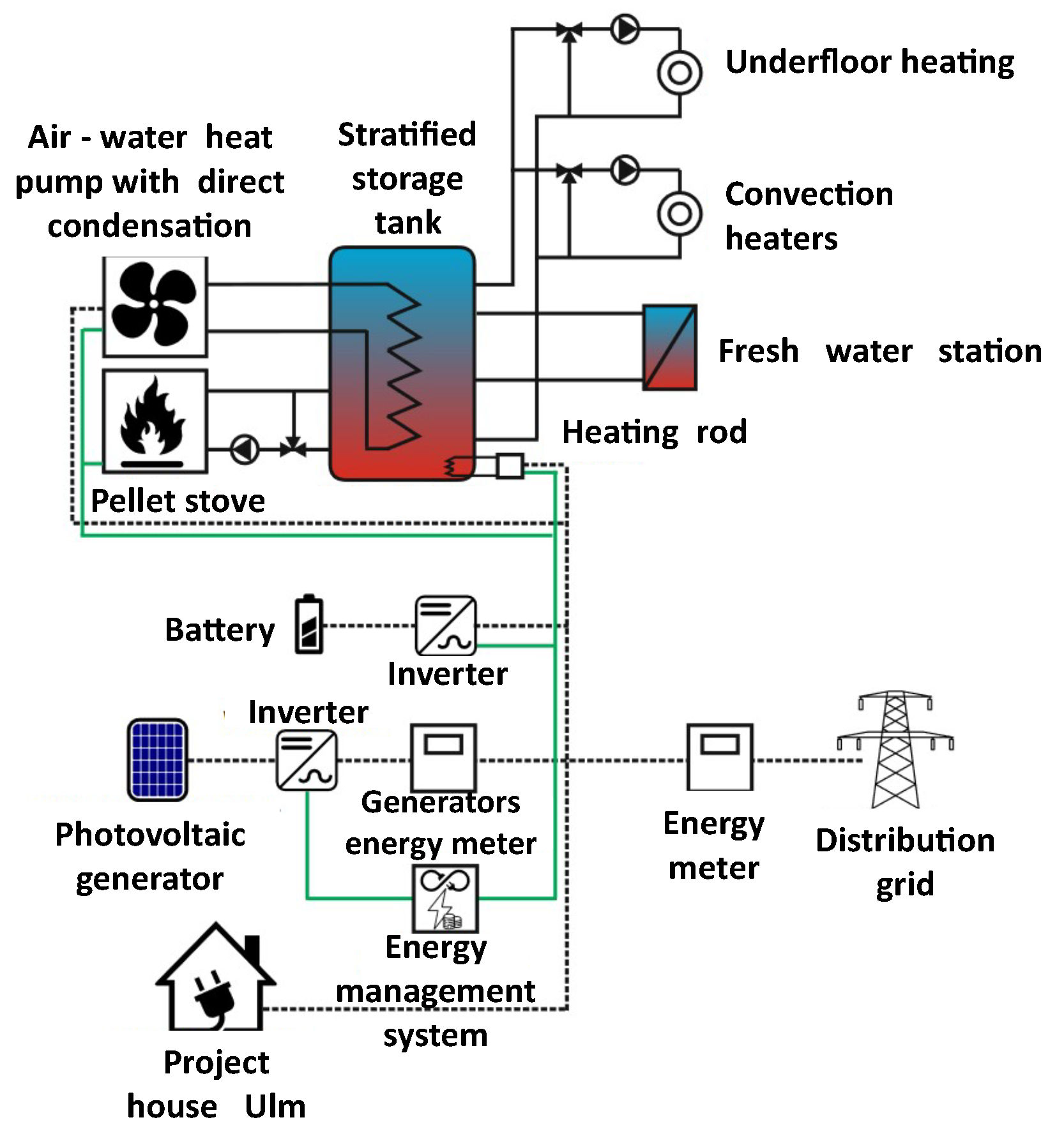
Figure 1. Schematic representation of the installed components in the Projekthaus Ulm [34]. Black lines represent the connections of the energy system, heat as full lines, and electricity as dashed lines. Green lines represent key communication lines.
Energies 16 06980 g001
Figure 2. (Left): sky image from the camera at the Projekthaus, (middle): computed cloud mask with cloud motion vectors, (right): resulting irradiance forecast for the location of the Projekthaus.
Energies 16 06980 g002
Figure 3. Flow diagram of predictive heuristic control; a detailed description of the variables is defined in Section 2.4.1.
Energies 16 06980 g003
Figure 4. Hybrid model structure with LSTM neural network for the stratified thermal storage and linear regression model for the heat pump, showing input and output parameters.
Energies 16 06980 g004
Figure 5. Model predictive control implementation in Projekthaus Ulm.
Energies 16 06980 g005
Figure 6. Validation of ASI-based GHI and PV power forecasts and corresponding persistence forecasts for May and June 2019. Shown is the RMSE normalized with the average irradiance or power.
Energies 16 06980 g006
Figure 7. Validation of the intraday irradiance forecast (left) and PV power forecast (right) for May until August 2019. Shown is the RMSE normalized with the average irradiance or power.
Energies 16 06980 g007
Figure 8. PHC test real output on April 20.
Energies 16 06980 g008
Figure 9. MPC test results on 14 April.
Energies 16 06980 g009
Figure 10. MPC test results.
Energies 16 06980 g010
Figure 11. MPC prediction results. Each colored line represents the temperature of each of the 8 meassured layers in the storage tank. A full line depicts the real meassured value, a dashed line depicts the predicted temperature in each step calculated each iteration by the MPC.
Energies 16 06980 g011
Table 1. Validation of forecasted events for Δ t is 7 and 15 min for the forecast data set May–June 2019.
Δ t f c Δ t m e a s Events fcHitratePrecision
7 min7 min29590.9750.737
15 min7 min26550.9260.780
Disclaimer/Publisher’s Note: The statements, opinions and data contained in all publications are solely those of the individual author(s) and contributor(s) and not of MDPI and/or the editor(s). MDPI and/or the editor(s) disclaim responsibility for any injury to people or property resulting from any ideas, methods, instructions or products referred to in the content.