Reservoir Porosity Prediction Based on BiLSTM-AM Optimized by Improved Pelican Optimization Algorithm

Abstract

To accurately predict reservoir porosity, a method based on bi-directional long short-term memory with attention mechanism (BiLSTM-AM) optimized by the improved pelican optimization algorithm (IPOA) is proposed. Firstly, the nonlinear inertia weight factor, Cauchy mutation, and sparrow warning mechanism are introduced to improve the pelican optimization algorithm (POA). Secondly, the superiority of IPOA is verified by using the CEC–2022 benchmark test functions. In addition, the Wilcoxon test is applied to evaluate the experimental results, which proves the superiority of IPOA against other popular algorithms. Finally, BiLSTM-AM is optimized by IPOA, and IPOA-BiLSTM-AM is used for porosity prediction in the Midlands basin. The results show that IPOA-BiLSTM-AM has the smallest prediction error for the verification set samples (RMSE and MAE were 0.5736 and 0.4313, respectively), which verifies its excellent performance.

1. Introduction

Logging data are commonly used to predict reservoir parameters, including porosity, permeability, and oil and gas saturation. Generally, logging or core data are used to determine these reservoir properties. However, the evaluation of reservoir parameters is insufficient due to the relatively limited reservoir data that are acquired via logging and coring. Usually, a simplified geologic model or empirical formulas are established to estimate the reservoir parameters of an unknown interval [1]. But because of the very heterogeneous strata and complex geologic circumstances, the logging data frequently show a strong nonlinear characteristic, and the relative relationship between various data is complicated [2].

With the advent of the data-driven era and the popularity of digital oilfield, a great number of rock property parameters can be obtained through logging technology. The use of machine learning algorithms in the geophysics field, including in petrophysical property evaluation [3], first-break picking [4], and lithology identification [5], has become a major trend. Artificial neural networks (ANNs) and back-propagation neural networks (BPNNs) have been used many times to predict logging data [6]. These neural networks are fully connected, with separate, unconnected neurons existing in the same layer. When predicting reservoir parameters, logging data from depths greater than or equal to the depth of interest is not taken into account, and the accuracy of the anticipated result is not always guaranteed. When dealing with massive data, ANN and BPNN have poor accuracy and are prone to falling into the local minimum. From the standpoint of network architecture, one drawback of ANN and BPNN is that the information retrieved cannot be sent across layers. Therefore, using ANN and BPNN to predict sequence data effectively is challenging. Many academics use advances in ANN and BPNN to make predictions, but putting these networks into practice is a very difficult task [7].

Deep learning is one of the main areas of machine learning research at the moment. Numerous scientific domains have witnessed breakthrough accomplishments in deep learning [8]. Deep learning-based prediction accuracy is constantly improving, and an increasing number of real-world development issues are being addressed with deep learning techniques. A lot of experimental investigations have verified that diverse data representations significantly influence the accuracy of task learning [9]. And deep learning can be applied to the solution of challenging nonlinear geological issues [10]. However, the original deep learning methods only take into account the relationship between the logging data at different points at the same depth, ignoring the trend and correlation of the logging data with formation depth. A recurrent neural network (RNN) incorporates the timing idea into its architecture to improve the accuracy of the sequential data representation [11]. The long short-term memory (LSTM) model is a modified version of RNN that efficiently solves the gradient dispersion and exploding gradient issues in RNN through the use of a special model structure. The inability of RNN to remember feature information over an extended period of time during training and learning is another issue that LSTM can resolve. LSTM uses implicit unit neurons, which is a type of information transmission mechanism similar to that of organismal neurons. Therefore, LSTM can take into consideration the variation trend of the log sequence data with depth in addition to utilizing the internal relationships among different logging sequences [12]. However, LSTM can only make use of the correlation of logging data information in a single direction. Bi-directional long short-term memory (BiLSTM) can extract the features of the logging sequence from the front and back, respectively, along the depth, and make full use of the dependent information in the front and back sequences to predict the reservoir porosity [13]. Further, the attention mechanism is integrated into the hidden state by mapping weight value to strengthen the influence of important information [14].

It has been demonstrated that the pelican optimization algorithm (POA) provides outstanding optimization performance [15]. However, it also has the disadvantages of unbalanced global exploration and easily falling into local optimum. The nonlinear inertia weight factor, Cauchy mutation strategy, and sparrow warning mechanism are introduced to improve the optimization ability and convergence speed. It can be found that IPOA-BiLSTM-AM has more remarkable porosity prediction performance than the rival machine learning methods, which provides a promised way for predicting porosity. The remainder of this paper is organized as follows. Section 2 presents the principle of IPOA. Section 3 presents the superiority of IPOA by using the CEC–2022 benchmark test functions. Section 4 presents the practical application and result analysis of IPOA-BiLSTM-AM by using the NMR porosity data in the Midlands basin. Finally, the paper is concluded in Section 5.

2. Principle and Modeling

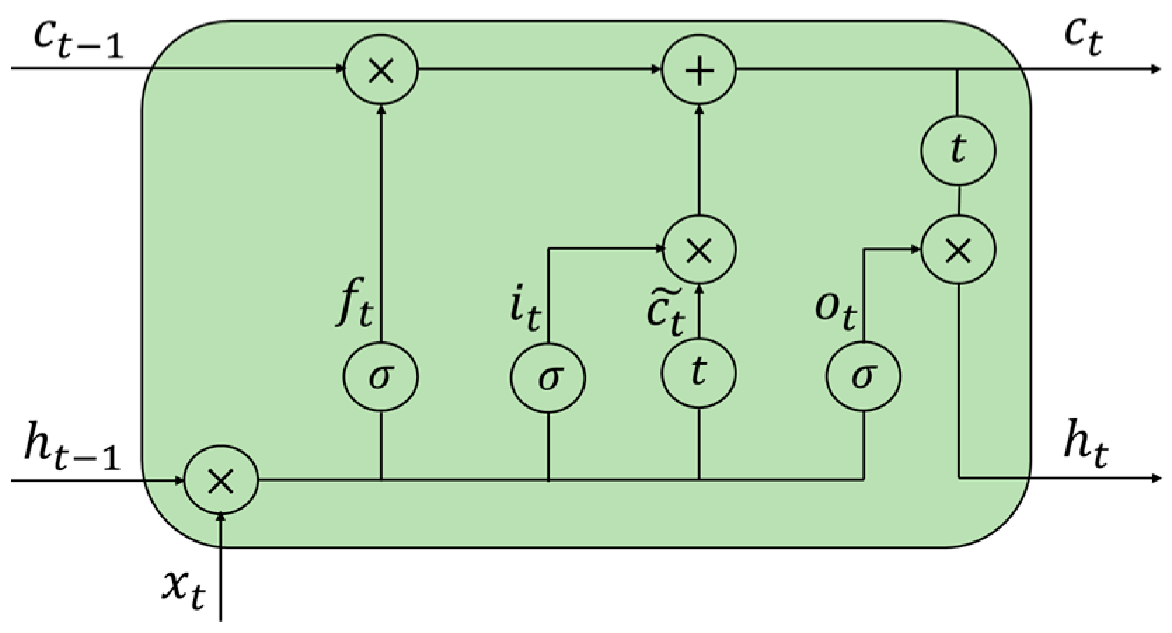
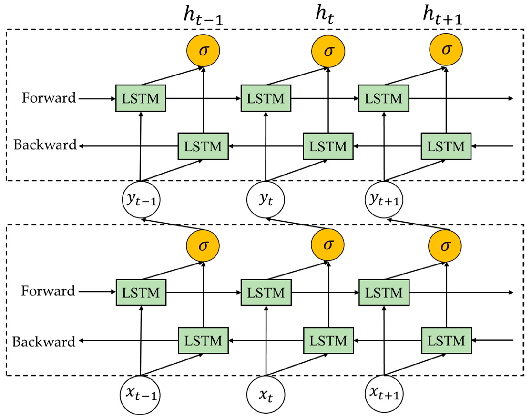
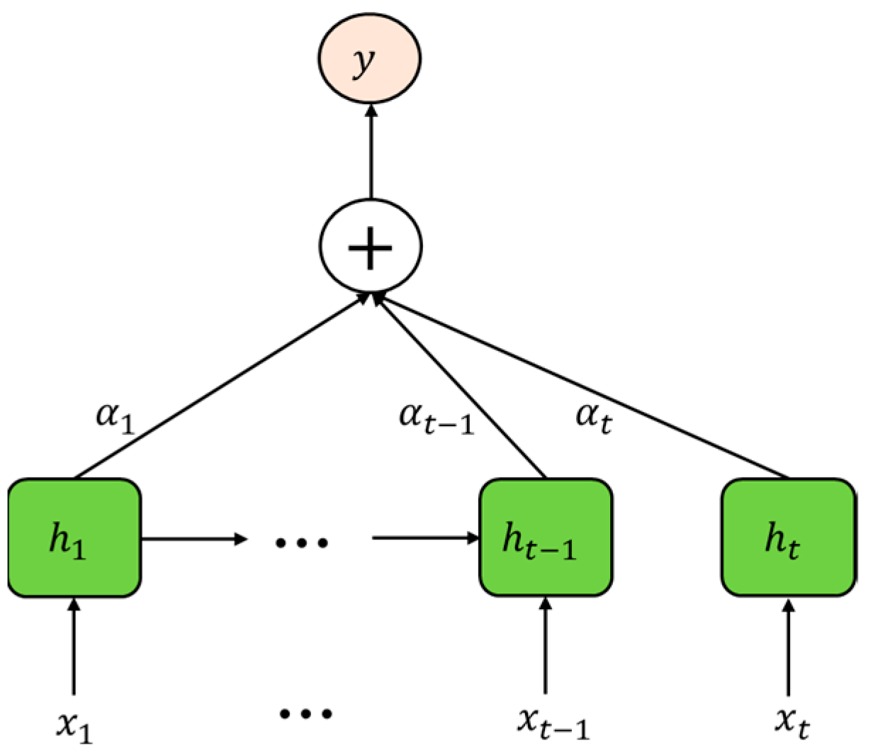
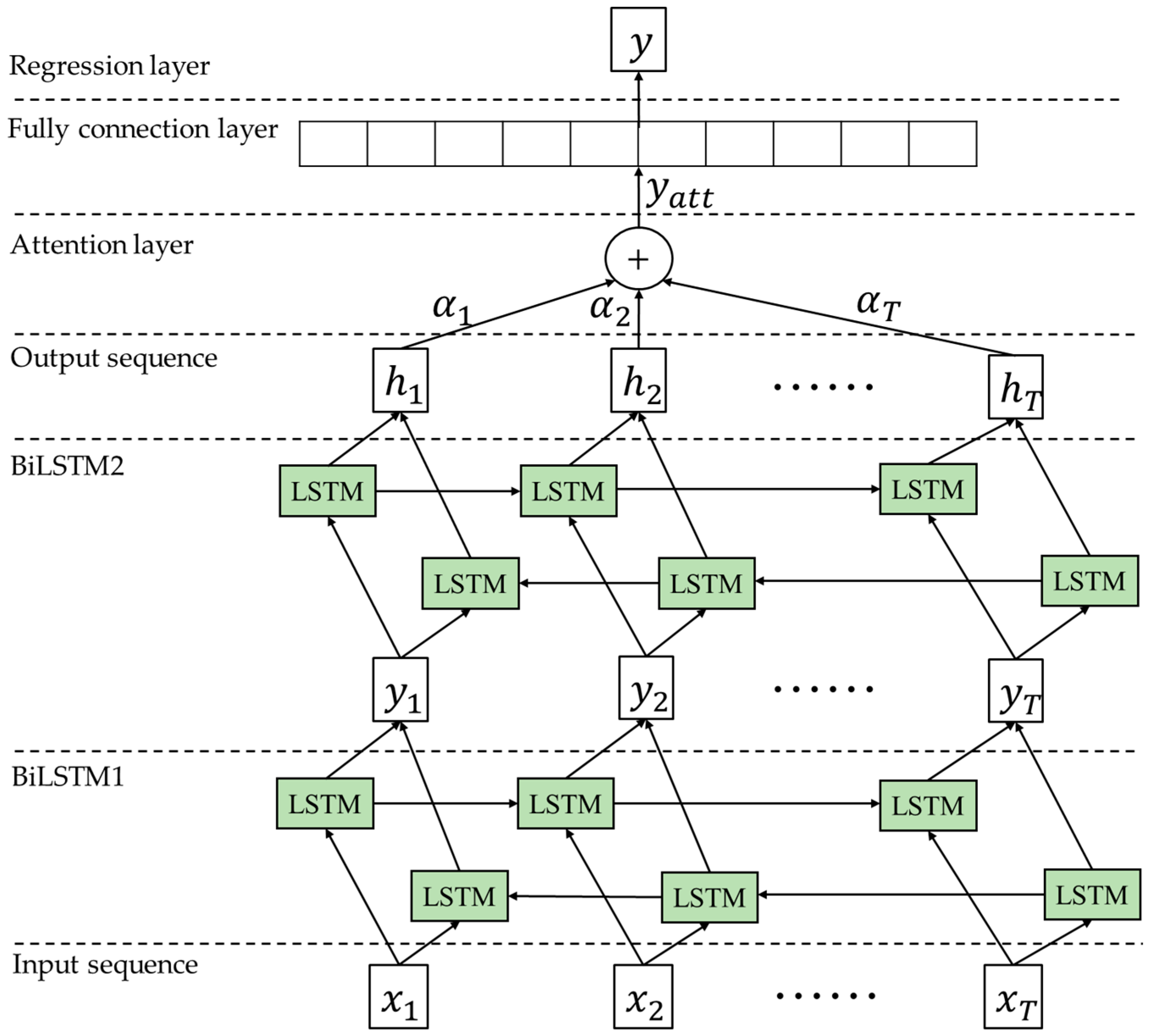
2.1. Principle of BiLSTM-AM

The long short-term memory neural network (LSTM) is an improved recurrent neural network (RNN). By using an LSTM network memory cell, the issue of RNN gradients inflating or disappearing has been resolved. The input, output, and forget gates are the three nodes that make up the hidden layer, which is constructed by the memory cells. The gates operate selectively, allowing specific data to be saved for further processing and enabling the LSTM network to avoid vanishing gradients. LSTM is able to retain information because the weights of the memory cells are adjusted during backpropagation. As a result, when long-term dependencies between input and output are needed, LSTM networks perform admirably. The basic structural unit of LSTM network is shown in Figure 1.

The following represents the mathematical formulations of the associated gates of the LSTM cell for an input sequence ($X=[x_1,x_2,\dots ,x_n]$) that is mapped to an output ($h=[h_1,h_2,\dots ,h_n]$) that results from the network being activated repeatedly for $t=[\mathrm{1,2},\dots ,t-1,\dots ,T]$:

$$i_t=\sigma (w_{ix}{x}_t+w_{ih}{h}_{t-1}+b_i)$$

(1)

$$f_t=\sigma (w_{fx}{x}_t+w_{fh}{h}_{t-1}+b_f)$$

(2)

$$g_t=\phi (w_{gx}{x}_t+w_{gh}{h}_{t-1}+b_g)$$

(3)

$$o_t=\sigma (w_{ox}{x}_t+w_{oh}{h}_{t-1}+b_o)$$

(4)

$$c_t=\sigma (g_t⨁i_t+w_{ih}⨁c_{t-1})$$

(5)

$$h_t=\phi \left(c_t\right)⨁o_t$$

(6)

where $w$ and $b$ represent the weight matrices and the bias, respectively; $i_t$, $f_t$, and $o_t$ are the input gate, forget gate, and output gate, respectively; $c_t$ and $h_t$ are the cell state and hidden state, respectively; and $\phi$ and $\sigma$ denote tanh and sigmoid activation functions, respectively.

To enhance the performance of a single LSTM cell, a bi-directional recurrent network (BiLSTM) that combines two hidden layers of LSTM is developed. After processing the input sequence ($X=[x_1,x_2,\dots ,x_n]$), BiLSTM produces hidden sequences in both the forward ($\overrightarrow{h_t}=[\overrightarrow{h_1},\overrightarrow{h_2},\dots ,\overrightarrow{h_n}]$) and backward ($\overleftarrow{h_t}=[\overleftarrow{h_1},\overleftarrow{h_2},\dots ,\overleftarrow{h_n}]$) directions. Concatenating the forward and backward hidden outputs yields the final output. The encoded vector arising from the two hidden levels can be expressed mathematically as follows:

$$y_t=\sigma (w_{y\overrightarrow{h}}\overrightarrow{h_t}+w_{y\overleftarrow{h}}\overleftarrow{h_t}+b_y)$$

(7)

$$\overrightarrow{h_t}=\sigma (w_{\overrightarrow{h}x}{x}_t+w_{\overrightarrow{h}\overrightarrow{h}}\overrightarrow{h_{t-1}}+b_{\overrightarrow{h}})$$

(8)

$$\overleftarrow{h_t}=\sigma (w_{\overleftarrow{h}x}{x}_t+w_{\overleftarrow{h}\overleftarrow{h}}\overleftarrow{h_{t+1}}+b_{\overleftarrow{h}})$$

(9)

where $y_t=[\overrightarrow{h_t},\overleftarrow{h_t}]$ is the output of the network’s corresponding sequence for the first hidden layer. The output of the previous layer of the stacking BiLSTM becomes the input of its succeeding layer. The structure of BiLSTM is shown in Figure 2.

An attention mechanism (AM) is a data processing method that can ignore useless information and amplify useful information through clever and reasonable allocation. An AM is introduced into the BiLSTM structure to assign different weights to feature vectors and focus attention to highlight key features, and better results can be obtained. The attention mechanism structure is shown in Figure 3.

In Figure 3, $x_t$ is BiLSTM’s input, $h_t$ is the hidden layer output produced by BiLSTM, and ${\alpha }_t$ is the attention probability distribution of BiLSTM hidden layer’s attention mechanism output. The attention layer input is the output vector that the BiLSTM activation layer processes, and the weight coefficient of the attention layer is obtained as follows:

$$e_t=utanh\left(w{h}_t\right)$$

(10)

$${\alpha }_t=\frac{\mathrm{e}\mathrm{x}\mathrm{p}\left(e_t\right)}{{\sum }_{j=1}^t{e}_j}$$

(11)

$$y_{att}=\sum _{t=1}^i{\alpha }_t{h}_t$$

(12)

where $e_t$ is the value of the attention probability distribution computed by the LSTM output vector $h_t$, $u$ and $w$ are the weight coefficients, and $s_t$ is the attention layer output. The final output $y_{att}$ is a representation of the input’s high-level abstract information.

The network structure of BiLSTM-AM is shown in Figure 4.

It can be seen from Figure 4 that two BiLSTM layers are stacked on top of each other. Figure 4 illustrates how input information propagates both forward and backward in each BilLSTM structure. The input of BiLSTM2 is the output of BiLSTM1. The final hidden states are multiplied by attention weights and summated to provide the network’s final output. The incorporation of an attention mechanism facilitates the extraction of highly relevant information from input sequences with a long range. The regression layer uses the attention layer’s output to obtain the result of regression prediction.

2.2. Pelican Optimization Algorithm

Pelican optimization algorithm (POA) is a heuristic intelligent optimization algorithm proposed by Pavel Trojovský and Mohammad Dehghani in 2022 [6]. It is inspired by the natural behavior of pelicans during hunting and modeled by simulating the moving towards prey (exploration phase) and winging on the water surface (exploitation phase).

2.2.1. Moving towards Prey (Exploration Phase)

The first phase involves the pelicans locating the prey and then making their way toward it. Search space scanning and the exploration capability of POA in locating various search space regions are made possible by modeling the pelican’s approach. The pelican’s approach to the prey location can be defined by Equation (13):

$$x_{i,j}^{P_1}=\left\{\begin{array}{c}{x}_{i,j}+rand·\left(p_j-I·x_{i,j}\right),F_p<F_i;\\ x_{i,j}+rand·\left(x_{i,j}-p_j\right),else,\end{array}\right.$$

(13)

where $x_{i,j}^{P_1}$ represents the $i$th pelican’s new status in the jth dimension, $I$ is a random number that can be either 1 or 2, $p_j$ is the location of prey in the $j$th dimension, and $F_p$ is its objective function value.

In POA, if the value of the objective function is improved at the current position, the new position of the pelican is accepted; otherwise, it is not. This update method prevents the algorithm from moving to a non-optimal region. The process can be described using Equation (14):

$$X_i=\left\{\begin{array}{c}{X}_i^{P_1},F_i^{P_1}<F_i;\\ X_i,else,\end{array}\right.$$

(14)

where $X_i^{P_1}$ represents the new status of the $i$th pelican, and $F_i^{P_1}$ is the pelican’s objective function in the first phase.

2.2.2. Winging on the Water Surface (Exploitation Phase)

In the second phase, when the pelicans reach the water’s surface, they spread their wings on the surface of the water to move the fish upwards, then collect the prey in their throat pouch. This strategy leads more fish in the attacked area to be caught by pelicans. This behavior of pelicans causes POA to converge to better points in the hunting area. The behavior of pelicans during hunting can be defined by Equation (15):

$$x_{i,j}^{P_2}=x_{i,j}+R·(1-\frac{t}{T})·(2·rand-1)·x_{i,j}$$

(15)

where $x_{i,j}^{P_2}$ represents the $i$th pelican’s new status in the $j$th dimension based on phase 2, $R$ is a constant with a value of $0.2$, $T$ is the maximum iteration number, and $t$ is the current iteration number. $R·(1-\frac{t}{T})$ represents the radius of the neighborhood where each population member is located in order to search locally and converge on a better solution.

At this phase, the new pelican position has also been accepted or rejected using effective updating, which can be represented by Equation (16):

$$X_i=\left\{\begin{array}{c}{X}_i^{P_2},F_i^{P_2}<F_i;\\ X_i,else,\end{array}\right.$$

(16)

where $X_i^{P_2}$ represents the new status of the $i$th pelican, and $F_i^{P_2}$ is the pelican’s objective function in the second phase.

By updating every member of the population according to the first and second phases, the optimal candidate solution will be updated, taking into account the population’s new status and the objective function’s values. The algorithm then moves on to the following iteration, repeating the various stages of POA based on Equations (13)–(16) until the execution is finished. Lastly, a quasi-optimal solution to the given problem is offered using the best candidate solution found. POA has the characteristics of faster optimization speed and good convergence accuracy and has fewer parameters, is simple to operate, and has a wide application range. However, some problems remain, such as decreasing convergence speed and falling into local extremum in the late iteration.

2.3. Improvement of POA

2.3.1. Nonlinear Inertia Weight Factor

Coordinating the local and global optimization ability is the key factor that can affect the optimization accuracy and speed. Since the updating of a pelican’s individual position is closely related to the current position, the nonlinear inertia weight factor $\omega$ can be used to adjust the correlation between the updated position and the current position information of the pelican. The calculation method of the nonlinear inertia weight factor is as follows:

$$\omega =\frac{e^{\frac{t}{T}}-1}{e-1}$$

(17)

where $T$ is the maximum iteration number, and $t$ is the current iteration number. In the initial iteration of the algorithm, $\omega$ is small, and the updating of the position of the seeking individual is less affected by the current position of the pelican, which is conducive to the search of the algorithm in a larger scope and improve the global development ability of the algorithm. With the advancement of the optimization process, $\omega$ gradually increases, and the update of the position of the optimization individual becomes more influenced by the pelican’s current position. Narrowing the optimization range of the algorithm helps the algorithm search for the optimal solution, which not only improves the local exploration ability but also improves the convergence speed. The pelican’s approach to the prey’s location can be improved with Equation (18):

$$x_{i,j}^{P_1}=\left\{\begin{array}{c}{\omega ·x}_{i,j}+rand·\left(p_j-I·x_{i,j}\right),F_p<F_i;\\ \omega ·x_{i,j}+rand·\left(x_{i,j}-p_j\right),else,\end{array}\right.$$

(18)

2.3.2. Cauchy Mutation

The Cauchy mutation strategy is introduced to improve the optimization ability of POA in the second phase. Each iteration compares the size of the current pelican’s fitness value with the population average fitness value. When the current fitness value is lower than the average fitness value of the population, it indicates that the current pelicans are in an aggregative state. In this case, Cauchy variation strategy is adopted to increase pelican diversity. When the current fitness value is higher than the average fitness value of the population, the original pelican location updating method is used. The behavior of pelicans during hunting can be improved with Equation (19):

$$x_{i,j}^{P_2}=\left\{\begin{array}{c}{x}_{best}+x_{best}·Cauchy\left(\mathrm{0,1}\right),F_i^{P_2}<F_{avg}\\ x_{i,j}+R·\left(1-\frac{t}{T}\right)·\left(2·rand-1\right)·x_{i,j},else\end{array}\right.$$

(19)

where $F_i^{P_2}$ is the current fitness value in the second phase, $F_{avg}$ is the average fitness value of the population, and $x_{best}$ is the optimal fitness value of the population.

2.3.3. Sparrow Warning Mechanism

The presence of predators makes sparrows very sensitive and cautious. When a host of sparrows becomes aware of danger, those on the edge of the host quickly move to safety to obtain a better position, while those in the middle of the host move randomly to come closer to other sparrows. Therefore, the sparrow host can be integrated with the sparrow’s warning mechanism, which can make the meta-heuristic algorithm improve convergence speed. Therefore, the sparrow alert mechanism can be applied to improve the optimization ability of POA in the second phase. The sparrow mechanism can be obtained from Equation (20):

$$x_{i,j}^{P_2}=\left\{\begin{array}{c}{x}_{best}+b·\left|x_{i,j}-x_{best}\right|F_i^{P_2}>F_g\\ x_{i,j}+k·\left(\frac{x_{i,j}-x_{\mathrm{worst}}}{\left(F_i^{P_2}-F_w\right)+\epsilon }\right)F_i^{P_2}=F_g\end{array}\right.$$

(20)

where $x_{best}$ is the current global optimal location; $b$ is a random number with a normal distribution of mean 0 and variance 1; $k$ is a random number between [−1,1]; $F_i^{P_2}$ is the fitness value of the current individual pelican; $F_g$ and $F_w$ are the best and worst global fitness values, respectively; and $\epsilon$ is a constant to avoid zeros in the denominator. $F_i^{P_2}>F_g$ indicates that the pelican is at the edge of the population and is vulnerable to natural enemies. When $F_i^{P_2}=F_g$, it indicates that the pelican in the middle of the swarm is aware of the danger and needs to stay close to other pelicans to avoid predation.

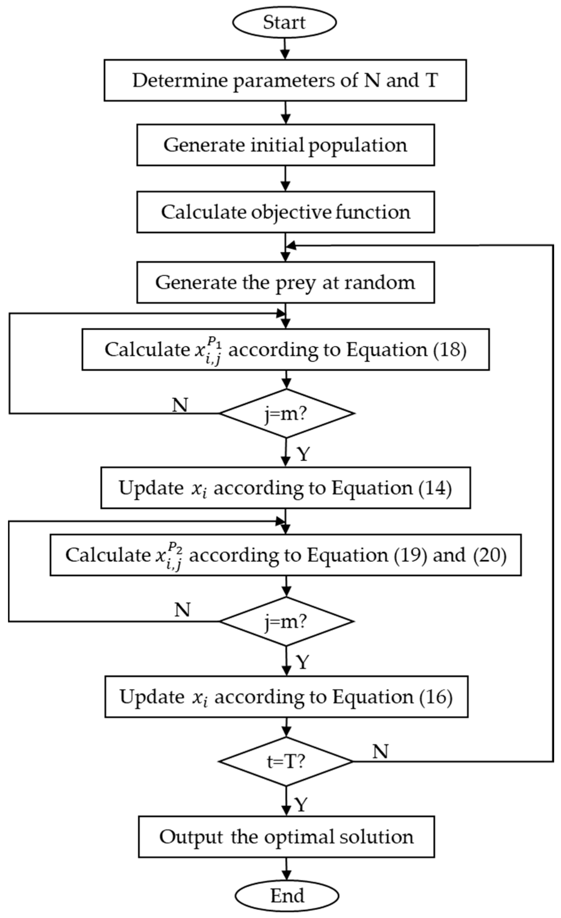
2.3.4. IPOA Calculation Flow

The IPOA calculation flow is shown in Figure 5.

The overall steps of IPOA are as follows:

• Step 1: set population size $N$, maximum number of iterations $T$.
• Step 2: generate initial population.
• Step 3: calculate objective function.
• Step 4: generate the prey at random.
• Step 5: calculate $x_{i,j}^{P_1}$ according to Equation (18).
• Step 6: update the $X_i$ position according to Equation (14).
• Step 7: calculate $x_{i,j}^{P_2}$ according to Equations (19) and (20).
• Step 8: update the $X_i$ position according to Equation (16).
• Step 9: determine whether the end condition is reached; if so, jump to the next step; otherwise, jump to step 4.
• Step 10: output the optimal solution.

3. IPOA Performance Test

In this section, the CEC–2022 benchmark test functions are employed to examine the efficiency of IPOA. To compare the performance of IPOA with the rival algorithms, including sand cat swarm optimization (SCSO) [16,17], dung beetle optimizer (DBO) [18], sparrow search algorithm (SSA) [19,20], and whale optimization algorithm (WOA) [21], the population size and maximum iteration number are 30 and 500, respectively, in addition to the average value of each objective function derived from 30 separate runs for each algorithm.

3.1. Exploration and Exploitation Analysis

The test results of IPOA and other algorithms are shown in

Table 1. Results of IPOA, POA, SCSO, DBO, SSA, and WOA on CEC–2022 benchmark functions. The standard deviation is presented in parentheses and the best values are written in bold.

Funciton	IPOA	POA	SCSO	DBO	SSA	WOA
F1	3.29 × 102	7.34 × 102	3.07 × 103	3.68 × 103	5.26 × 103	4.12 × 103
	(1.37 × 102)	(8.84 × 102)	(2.36 × 103)	(1.90 × 103)	(2.25 × 103)	(2.26 × 103)
F2	4.22 × 102	4.28 × 102	4.45 × 102	4.55 × 102	4.66 × 102	4.58 × 102
	(2.95 × 101)	(3.04 × 101)	(3.54 × 101)	(3.43 × 101)	(3.62 × 101)	(3.18 × 101)
F3	6.06 × 102	6.19 × 102	6.17 × 102	6.24 × 102	6.22 × 102	6.10 × 102
	(4.72 × 100)	(9.68 × 100)	(1.06 × 101)	(5.54 × 100)	(1.07 × 101)	(5.55 × 100)
F4	8.13 × 102	8.19 × 102	8.28 × 102	8.23 × 102	8.47 × 102	8.31 × 102
	(6.59 × 100)	(4.44 × 100)	(5.17 × 100)	(6.56 × 100)	(7.25 × 100)	(1.04 × 101)
F5	1.16 × 103	1.09 × 103	1.13 × 103	1.05 × 103	9.79 × 102	1.02 × 103
	(2.21 × 102)	(1.21 × 102)	(2.01 × 102)	(7.86 × 101)	(4.88 × 101)	(1.14 × 102)
F6	4.57 × 102	2.79 ×103	4.48 × 103	2.23 × 103	5.17 × 104	1.43 × 104
	(2.44 × 102)	(1.40 × 103)	(2.23 × 103)	(5.67 × 102)	(3.63 × 104)	(1.43 × 104)
F7	2.03 × 103	2.03 × 103	2.05 × 103	2.05 × 103	2.08 × 103	2.05 × 103
	(9.43 × 100)	(1.06 × 101)	(2.26 × 101)	(1.17 × 101)	(3.70 × 101)	(2.42 × 101)
F8	2.22 × 103	2.22 × 103	2.23 × 103	2.23 × 103	2.25 × 103	2.23 × 103
	(2.06 ×100)	(7.45 × 100)	(4.11 × 100)	(7.87 × 100)	(2.23 × 101)	(3.82 × 100)
F9	2.53 × 103	2.54 × 103	2.59 × 103	2.56 × 103	2.64 × 103	2.60 × 103
	(1.92 × 10−1)	(2.77 × 101)	(4.48 × 101)	(1.42 × 101)	(4.39 × 101)	(3.04 × 101)
F10	2.50 × 103	2.55 × 103	2.56 × 103	2.54 × 103	2.64 × 103	2.57 × 103
	(6.53 × 101)	(6.24 × 101)	(6.51 × 101)	(3.84 × 100)	(4.22 × 101)	(6.34 × 101)
F11	2.71 × 103	2.77 × 103	2.88 × 103	2.81 × 103	3.27 × 103	3.03 × 103
	(1.37 × 102)	(1.62 × 102)	(2.12 × 102)	(6.53 × 101)	(2.78 × 102)	(2.21 × 102)
F12	2.87 × 103	2.87 × 103	2.88 × 103	2.87 × 103	2.87 × 103	2.87 × 103
	(5.68 × 100)	(1.09 × 101)	(1.91 × 101)	(3.85 × 100)	(9.04 × 100)	(9.47 × 100)

, where the mean and the standard deviation of the fitness value are applied to assess the search accuracy and stability. IPOA finds the better solution when solving F1, F2, F3, F4, F6, F9, F10, and F11 functions. WOA is better at solving the function F5. For the functions F7 and F8, IPOA is the similar to POA but still better than the rest of the algorithms. For function F12, the search capability of all algorithms is reduced. Therefore, the above comparison shows the excellent performance of IPOA.

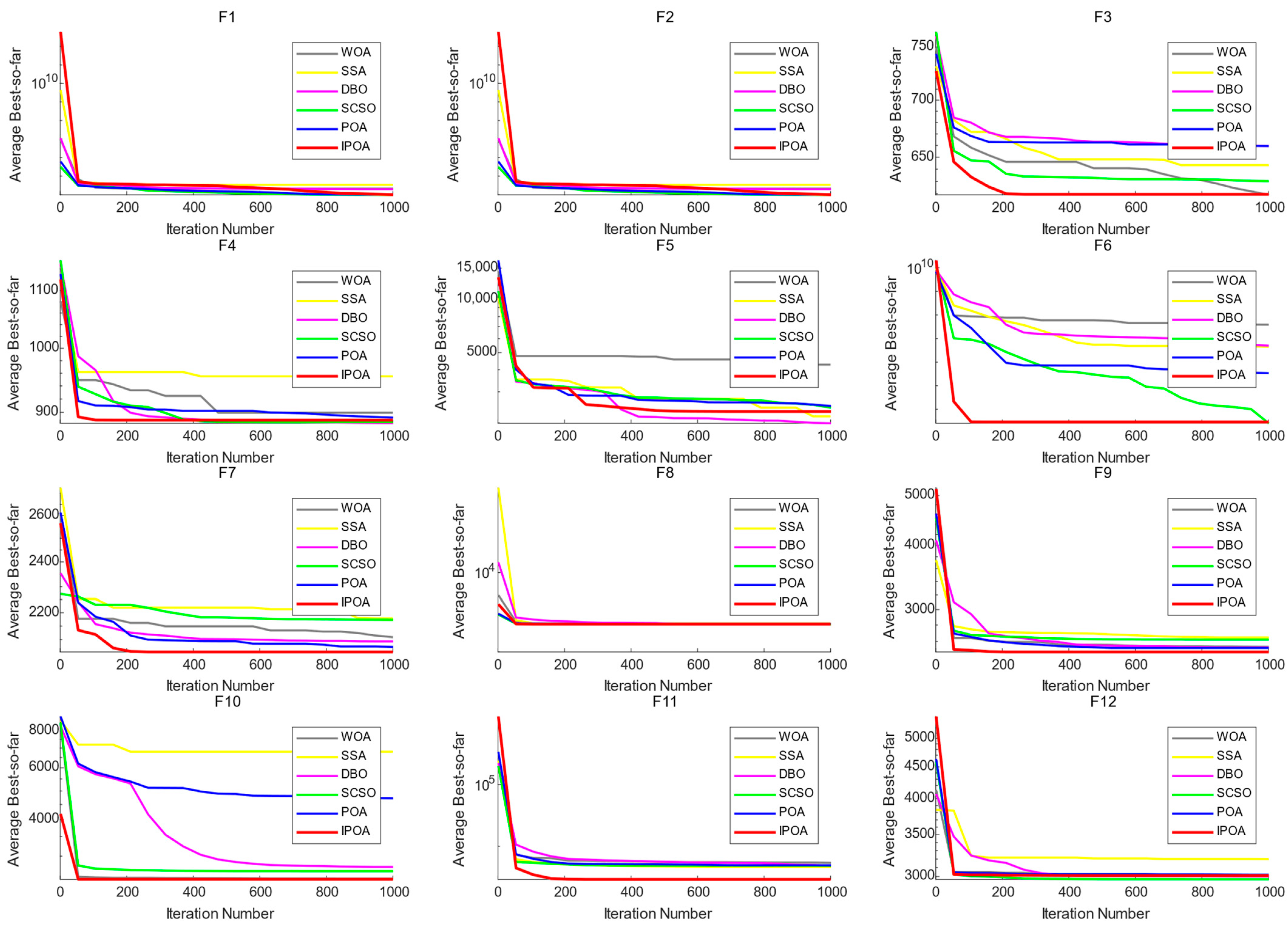
3.2. Comparative Analysis of Algorithm Convergence Curves

The performance of IPOA is analyzed with the convergence curve. Figure 6 shows the convergence curves of IPOA, POA, SCSO, DBO, SSA, and WOA algorithms on CEC–2022 benchmark functions. It can be concluded from Figure 6 that IPOA can acquire relatively satisfactory mean fitness values with a convergence that is more rapid than that of the other proposed algorithms in the iteration process.

3.3. Statistical Analysis Rank-Sum Test

In this section, the Wilcoxon test is used to further compare the distinctions between IPOA and the rival algorithms. The nonparametric Wilcoxon rank-sum tests’ p-values for the pairwise comparison between IPOA and the rival algorithms (SCSO, DBO, SSA, and WOA) are shown in

Table 2. Pair-wise comparison with IPOA and the rival algorithms.

Funciton	IPOA vs. POA		IPOA vs. SCSO		IPOA vs. DBO		IPOA vs. SSA		IPOA vs. WOA
	P	h	P	h	P	h	P	h	P	h
F1	1.29 × 10−9	+	8.15 × 10−11	+	3.02 × 10−11	+	3.34 × 10−11	+	3.69 × 10−11	+
F2	3.48 × 10−2	+	1.85 × 10−3	+	1.63 × 10−5	+	3.81 × 10−6	+	1.67 × 10−4	+
F3	6.01 × 10−8	+	4.42 × 10−6	+	4.50 × 10−11	+	1.17 × 10−9	+	5.57 × 10−3	+
F4	9.88 × 10−3	+	6.91 × 10−4	+	7.28 × 10−11	+	1.20 × 10−10	+	4.85 × 10−3	+
F5	6.52 × 10−1	−	9.00 × 10−1	−	3.87 × 10−1	−	2.71 × 10−2	+	8.50 × 10−2	−
F6	8.12 × 10−4	+	1.00 × 10−3	+	7.22 × 10−6	+	6.70 × 10−11	+	1.41 × 10−9	+
F7	6.57 × 10−2	−	8.56 × 10−4	+	2.88 × 10−6	+	1.61 × 10−10	+	1.95 × 10−3	+
F8	2.01 × 10−4	+	3.82 × 10−9	+	6.07 × 10−11	+	3.02 × 10−11	+	1.33 × 10−10	+
F9	9.67 × 10−9	+	5.04 × 10−11	+	2.25 × 10−11	+	2.25 × 10−11	+	2.25 × 10−11	+
F10	6.31 × 10−3	+	9.82 × 10−3	+	9.33 × 10−2	−	6.01 × 10−8	+	9.47 × 10−1	−
F11	2.60 × 10−3	+	1.17 × 10−4	+	3.33 × 10−3	+	9.62 × 10−10	+	5.99 × 10−7	+
F12	2.64 × 10−2	+	4.19 × 10−2	+	5.97 × 10−5	+	1.34 × 10−5	+	3.40 × 10−2	+

. In this table, the “+” denotes the proposed algorithm’s supremacy where p < 0.05 and the “−” indicates that the proposed algorithm’s obtained answer is inferior to the compared algorithms where p > 0.05.

The algorithm performance of IPOA and the rival algorithms is significantly different in F1, F2, F3, F4, F6, F8, F9, F11, and F12 functions. For function F5, the search capability of IPOA is similar to that of POA, SCSO, DBO, and WOA. For function F7, IPOA is similar to POA. For function F10, IPOA is similar to DBO. According to the above analysis, IPOA is generally superior to the rival algorithms.

4. Practical Application and Result Analysis

4.1. Construction of BiLSTM-AM Based on IPOA

In the training of BiLSTM-AM, IPOA is used to optimize the three parameters in BiLSTM-AM, including the number of nodes in the hidden layer, initial learning rate, and L2 regularization coefficient. In traditional model training, parameter selection is manually adjusted according to experience, which is greatly affected by subjective factors, so it is difficult to obtain the optimal model. Therefore, IPOA can be used to acquire the optimal combination of parameters, and the root mean square error (RMSE) is chosen as the fitness function. The specific steps of IPOA-BiLSTM-AM are as follows:

Step 1: Divide the input dataset into a training set and test set, and normalize the data to [0,1] using the max-min normalization method. The expression of the max-min normalization method is as follows:

$$x^{\prime }=\frac{x-x_{min}}{x_{max}-x_{min}}$$

(21)

where $x$ is the actual vector, $x_{max}$ and $x_{min}$ are the maximum and minimum values of the vector x, respectively, and $x^{\prime }$ is the normalized vector.

Step 2: Establish an objective function model. The objective function is the root-mean-square error (RMSE), which is expressed as follows:

$$RMSE=\sqrt{\frac{1}{N}{\sum }_{i=1}^N{\left(y_k-{\widehat{y}}_k\right)}^2}$$

(22)

where $y_k$ is the true value, and ${\widehat{y}}_k$ is the predicted value of BiLSTM-AM.

Step 3: IPOA is used to optimize the hyperparameters of BiLSTM-AM, and the optimal individual (the optimal parameters in BiLSTM-AM) is selected by judging the value of the fitness function or the maximum number of iterations.

Step 4: Apply the optimal combinations of the parameters to the estimation of BiLSTM-AM.

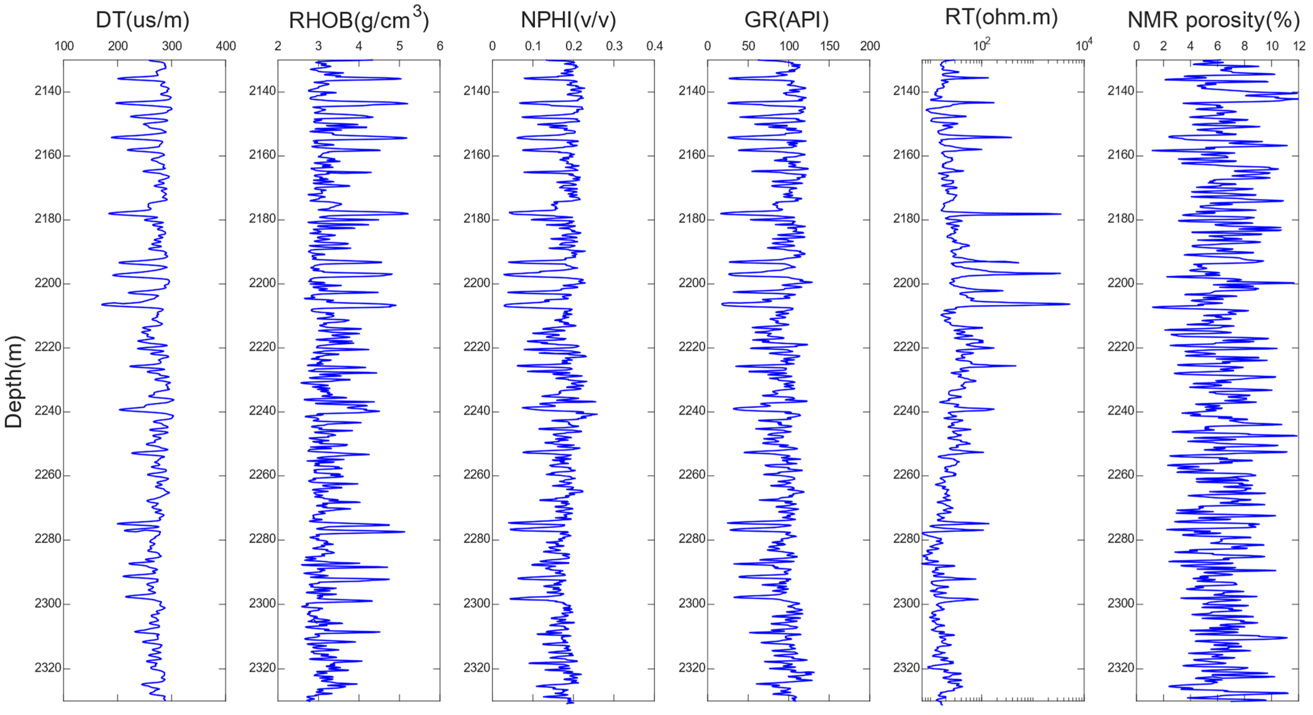
4.2. Data Preparation

Nuclear magnetic resonance logging (NMR) is an effective method to evaluate the porosity of a complex lithologic reservoir. The exploration well A with NMR, located in the Midlands basin, is studied. In addition, the Wolfcamp formation (2130–2330 m) is the interest interval of well A. The log graph for well A is shown in Figure 7. The included logging sequence is as follows: acoustic time difference (DT), density (RHOB), neutron porosity (NPHI), gamma ray (GR), true resistivity (RT), and the porosity derived by NMR (NMR porosity). It is important to note that due to data confidentiality requirements, we cannot present the original NMR graphs.

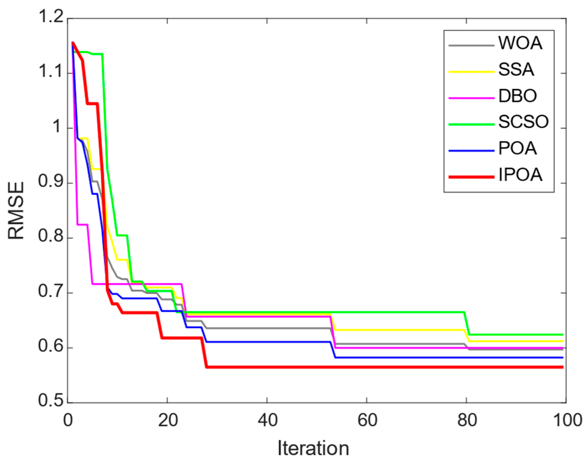
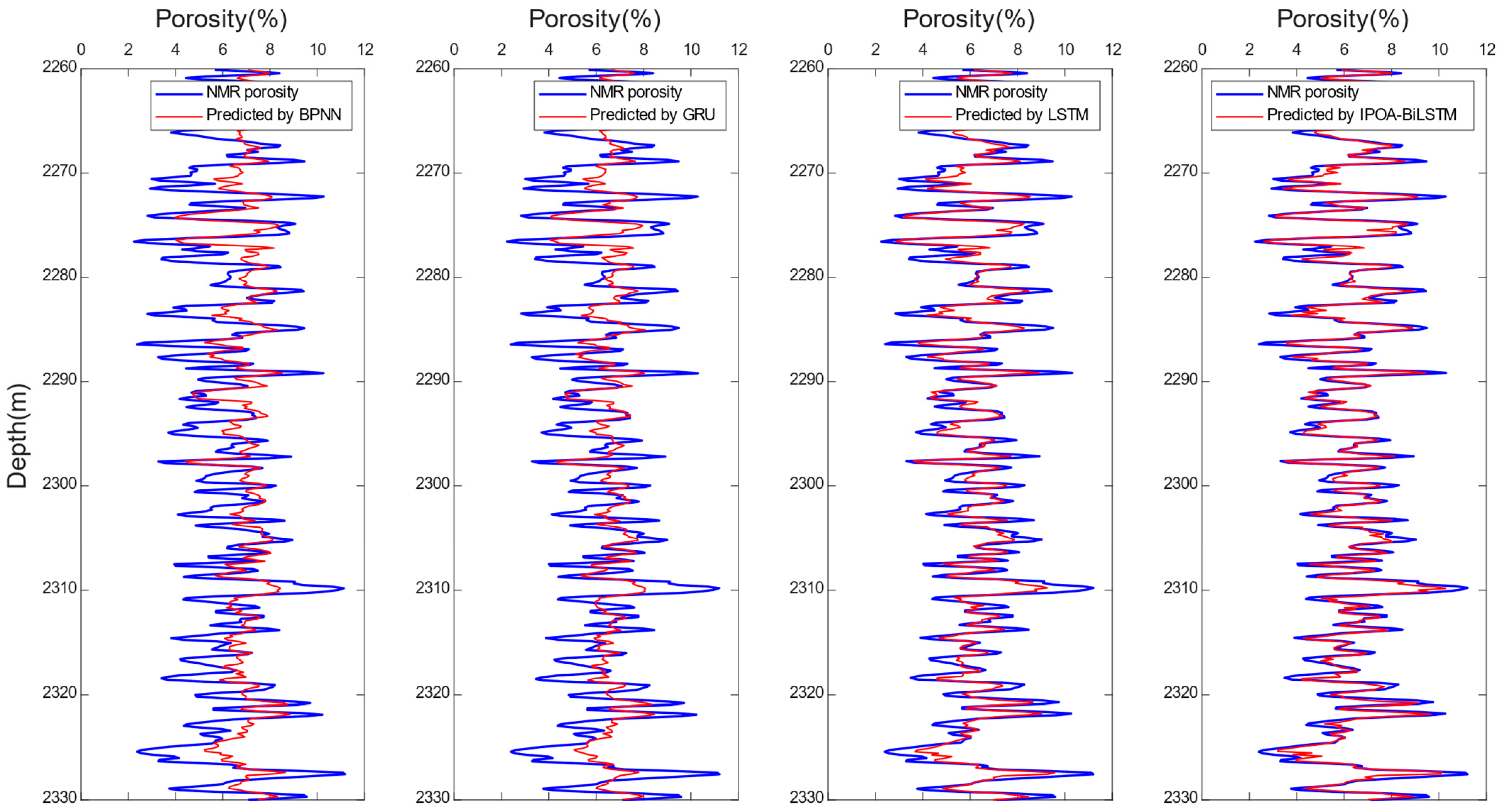
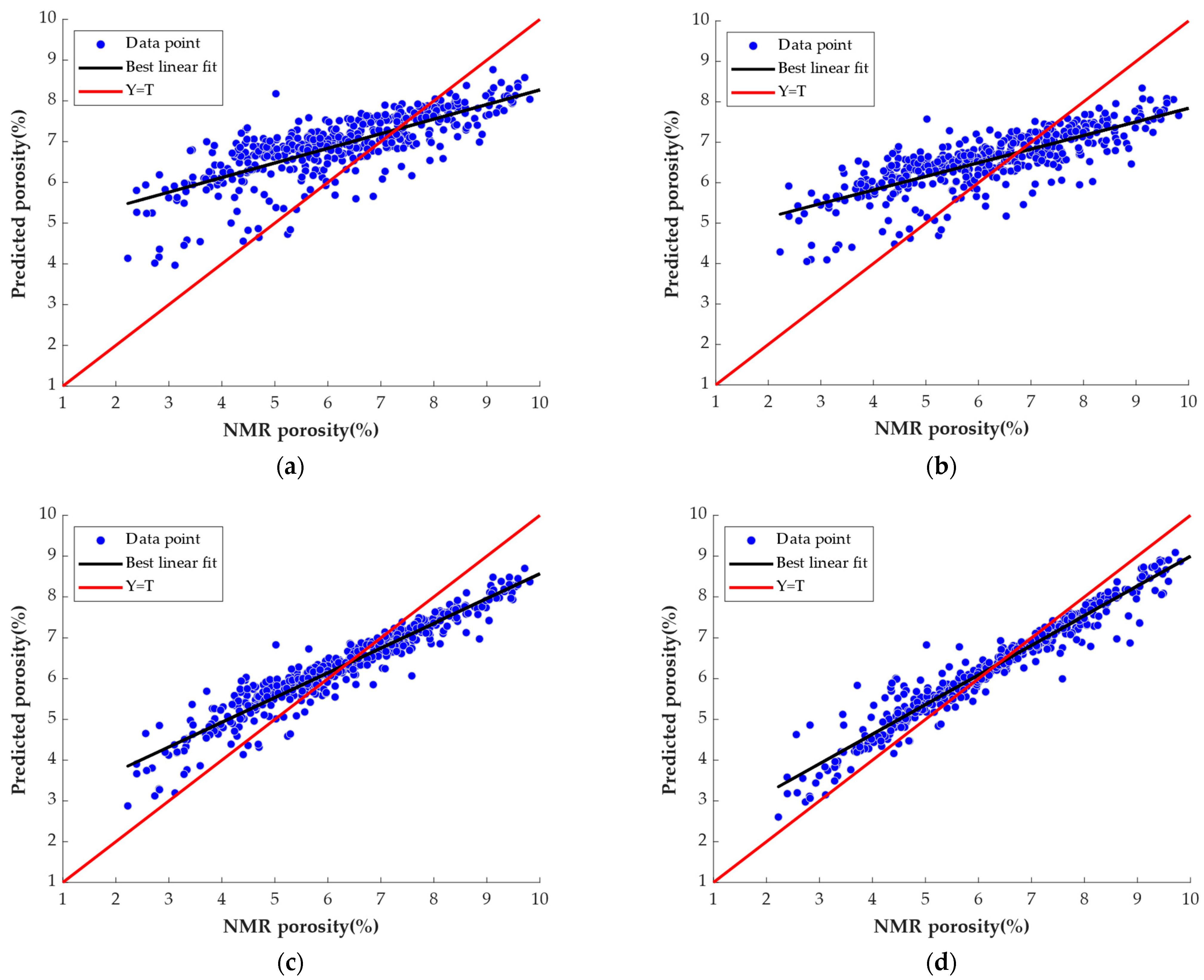
4.3. Analysis of Prediction Results

It is assumed that well A at depths from 2130 to 2260 m has the entire NMR porosity, which can be used as the training dataset to create IPOA-BiLSTM-AM and the rival models, including BPNN, the gated recurrent unit network (GRU), and LSTM. The six parameters (DEPTH, CAL, NPHI, GR, DT, and RT) serve as input parameters. The NMR porosity is the output parameter.

To prevent a huge search space from affecting optimization efficiency, the search range of relevant parameters is limited. Specifically, the L2 regularization coefficient is limited to 10⁻⁸–10⁻², the initial learning rate was limited to 10⁻⁴–10⁻³, and the number of nodes in the hidden layer is limited to 10–100. The fitness reduction rate in the training phase of BiLSTM-AM is shown in Figure 8. As can be observed, IPOA converges more quickly than the rival algorithms, and the final error resulting from IPOA is lower than those obtained from the rival algorithms. This further verifies the superiority of IPOA.

The parameter optimization results of IPOA are as follows: the number of nodes in the hidden layer is 60, the initial learning rate is 0.002, and the L2 regularization coefficient is 0.003. Using the trained model, the “missing” porosity of well A at depths from 2261 to 2330 m can be predicted. The quantitative prediction results of IPOA-BiLSTM-AM and the rival models are shown in

Table 3. Quantitative prediction results of IPOA-BiLSTM-AM and the rival models in well A at depths from 2261 to 2330 m.

Model	RMSE	MAE
BPNN	1.1217	1.0338
GRU	0.9712	0.9025
LSTM	0.7421	0.6918
IPOA-BiLSTM-AM	0.5736	0.4313

. It can be observed that IPOA-BiLSTM-AM has better prediction performance than the rival models.

The comparison between NMR porosity and estimated porosity in well A at depths from 2261 to 2330 m by the trained models is shown in Figure 9. The IPOA-BiLSTM-AM model’s prediction results are closer to the measured porosity, demonstrating that it is more appropriate for porosity prediction than the rival models.

The cross-plots of the NMR porosity versus predicted porosity utilizing IPOA-BiLSTM-AM, and the rival models are displayed in Figure 10.

It can be shown that the predicted porosity of IPOA-BiLSTM-AM is more in line with NMR porosity than the rival models, demonstrating that IPOA-BiLSTM-AM is more effective for porosity prediction. In conclusion, IPOA-BiLSTM-AM has an excellent effect on porosity prediction, clearly demonstrating its advantages.

5. Conclusions

In this paper, a reservoir porosity prediction method based on IPOA-BiLSTM-AM is proposed. BiLSTM-AM can fully extract the dependent information in the front and back sequences and strengthen the influence of important information. The nonlinear inertia weight factor, Cauchy mutation, and sparrow warning mechanism can improve the local exploration ability and the convergence speed of POA. In addition, IPOA-BiLSTM-AM is used for porosity prediction in the Midlands basin. In comparison to the rival models, IPOA-BiLSTM-AM has the fewest errors (RMSE: 0.5736 and MAE: 0.4313). Additionally, the estimated porosity of IPOA-BiLSTM-AM is more in line with NMR porosity than the rival models. Therefore, it can be confidently stated that IPOA-BiLSTM-AM is much better suited for porosity prediction.

References

1. Chen, Y.K. Automatic microseismic event picking via unsupervised machine learning. Geophys. J. Int. 2020, 3, 1750–1764. [Google Scholar] [CrossRef]
2. Chen, W.; Yang, L.Q.; Zha, B.; Zhang, M.; Chen, Y.K. Deep learning reservoir porosity prediction based on multilayer long short-term memory network. Geophysics 2020, 85, 213–225. [Google Scholar] [CrossRef]
3. Jia, B.; Xian, C.G.; Jia, W.F.; Su, J.Z. Improved Petrophysical Property Evaluation of Shaly Sand Reservoirs Using Modified Grey Wolf Intelligence Algorithm. Comput. Geosci. 2023, 27, 537–549. [Google Scholar] [CrossRef]
4. Chen, Y.K.; Zhang, G.Y.; Bai, M.; Zu, S.H.; Guan, Z.; Zhang, M. Automatic waveform classification and arrival picking based on convolutional neural network. Earth Space Sci. 2019, 6, 1244–1261. [Google Scholar] [CrossRef]
5. Silva, A.A.; Neto, I.A.L.; Roseane, M. Misságia.; Ceia, M.A.; Carrasquilla, A.G.; Archilha, N.L. Artificial neural networks to support petrographic classification of carbonate-siliciclastic rocks using well logs and textural information. J. Appl. Geophys. 2015, 117, 118–125. [Google Scholar] [CrossRef]
6. Mohebbi, A.; Kamalpour, R.; Keyvanloo, K.; Sarrafi, A. The prediction of permeability from well logging data based on reservoir zoning, using artificial neural networks in one of an iranian heterogeneous oil reservoir. Liq. Fuels Technol. 2012, 30, 1998–2007. [Google Scholar] [CrossRef]
7. Zheng, J.; Lu, J.R.; Peng, S.P.; Jiang, T.Q. An automatic microseismic or acoustic emission arrival identification scheme with deep recurrent neural networks. Geophys. J. Int. 2017, 212, 389–1397. [Google Scholar] [CrossRef]
8. Zhang, G.; Wang, Z.; Chen, Y. Deep learning for seismic lithology prediction. Geophys. J. Int. 2018, 215, 1368–1387. [Google Scholar] [CrossRef]
9. Zu, S.; Cao, J.; Qu, S.; Chen, Y. Iterative deblending for simultaneous source data using the deep neural network. Geophysics 2020, 85, 131–141. [Google Scholar] [CrossRef]
10. Duan, Y.X.; Xu, D.S.; Sun, Q.F.; Li, Y. Research and Application on DBN for Well Log Interpretation. J. Appl. Sci. 2018, 36, 689–697. [Google Scholar]
11. Zhang, D.X.; Chen, Y.T.; Jin, M. Synthetic well logs generation via Recurrent Neural Networks. Pet. Explor. Dev. 2018, 45, 629–639. [Google Scholar] [CrossRef]
12. Hochreiter, S.; Schmidhuber, J. Long short-term memory. Neural Comput. 1997, 9, 1735–1780. [Google Scholar] [CrossRef] [PubMed]
13. Chen, Y.; Liu, Z.; Zhang, Y.; Zheng, X.; Xie, J. Degradation-trend-dependent remaining useful life prediction for bearing with BiLSTM and attention mechanism. In Proceedings of the IEEE 10th Data Driven Control and Learning Systems Conference, Suzhou, China, 14–16 May 2021; pp. 1177–1182. [Google Scholar]
14. Wang, Y.; Jia, P.; Peng, X. BinVulDet: Detecting vulnerability in binary program via decompiled pseudo code and BiLSTM-attention. Comput. Secur. 2023, 125, 103023. [Google Scholar] [CrossRef]
15. Trojovsk, P.; Dehghani, M. Pelican Optimization Algorithm: A Novel Nature-Inspired Algorithm for Engineering Applications. Sensors 2022, 22, 855. [Google Scholar] [CrossRef] [PubMed]
16. Seyyedabbasi, A.; Kiani, F. Sand Cat swarm optimization: A nature-inspired algorithm to solve global optimization problems. Eng. Comput. 2022, 39, 2627–2651. [Google Scholar] [CrossRef]
17. Kiani, F.; Nematzadeh, S.; Anka, F.A.; Findikli, M.A. Chaotic Sand Cat Swarm Optimization. Mathematics 2023, 11, 2340. [Google Scholar] [CrossRef]
18. Xue, J.; Shen, B. Dung beetle optimizer: A new meta-heuristic algorithm for global optimization. J. Supercomput. 2022, 79, 7305–7336. [Google Scholar] [CrossRef]
19. Xue, J.; Shen, B. A novel swarm intelligence optimization approach: Sparrow search algorithm. Syst. Sci. Control Eng. 2020, 8, 22–34. [Google Scholar] [CrossRef]
20. Awadallah, M.A.; Al-Betar, M.A.; Doush, I.A. Recent Versions and Applications of Sparrow Search Algorithm. Arch. Comput. Methods Eng. 2023, 30, 2831–2858. [Google Scholar] [CrossRef] [PubMed]
21. Seyedali, M.; Andrew, L. The Whale Optimization Algorithm. Adv. Eng. Softw. 2016, 95, 51–67. [Google Scholar]
Figure 1. Structure of LSTM.
Energies 17 01479 g001
Figure 2. Structure of BiLSTM.
Energies 17 01479 g002
Figure 3. Attention mechanism structure.
Energies 17 01479 g003
Figure 4. Structure of BiLSTM-AM.
Energies 17 01479 g004
Figure 5. IPOA calculation flow.
Energies 17 01479 g005
Figure 6. Convergence curve analysis of IPOA and the rival algorithms in CEC–2022 test functions.
Energies 17 01479 g006
Figure 7. Logging graph of well A.
Energies 17 01479 g007
Figure 8. Fitness reduction rate in different iterations of IPOA for training BiLSTM-AM.
Energies 17 01479 g008
Figure 9. Logging graph of the measured and estimated RHOB in well A at depths from 2130 to 2330 m.
Energies 17 01479 g009
Figure 10. The cross-plot of measured porosity versus predicted porosity in well A at depths from 2261 to 2330 m. (a) BPNN; (b) GRU; (c) LSTM; (d) IPOA-BiLSTM-AM.
Energies 17 01479 g010