Communication

Comparative Analysis of Methods for Predicting Brine Temperature in Vertical Ground Heat Exchanger—A Case Study

by
Joanna Piotrowska-Woroniak
1,*,
Krzysztof Nęcka
2,*,
Tomasz Szul
2,* and
Stanisław Lis
2
1
Heating, Ventilation and Air Conditioning Department, Bialystok University of Technology, Wiejska 45E, 15-351 Bialystok, Poland
2
Faculty of Production and Power Engineering, University of Agriculture, Balicka 116 B, 30-149 Krakow, Poland
*
Authors to whom correspondence should be addressed.
Energies 2024, 17(6), 1465; https://doi.org/10.3390/en17061465
Submission received: 13 December 2023 / Revised: 25 January 2024 / Accepted: 15 March 2024 / Published: 19 March 2024

Abstract

:
This research was carried out to compare selected forecasting methods, such as the following: Artificial Neural Networks (ANNs), Classification and Regression Trees (CARTs), Chi-squared Automatic Interaction Detector (CHAID), Fuzzy Logic Toolbox (FUZZY), Multivariant Adaptive Regression Splines (MARSs), Regression Trees (RTs), Rough Set Theory (RST), and Support Regression Trees (SRTs), in the context of determining the temperature of brine from vertical ground heat exchangers used by a heat pump heating system. The subject of the analysis was a public building located in Poland, in a temperate continental climate zone. The results of this study indicate that the models based on Rough Set Theory (RST) and Artificial Neural Networks (ANNs) achieved the highest accuracy in predicting brine temperature, with the choice of the preferred method depending on the input variables used for modeling. Using three independent variables (mean outdoor air temperature, month of the heating season, mean solar irradiance), Rough Set Theory (RST) was one of the best models, for which the evaluation rates were as follows: CV RMSE 21.6%, MAE 0.3 °C, MAPE 14.3%, MBE 3.1%, and R2 0.96. By including an additional variable (brine flow rate), Artificial Neural Networks (ANNs) achieved the most accurate predictions. They had the following evaluation rates: CV RMSE 4.6%, MAE 0.05 °C, MAPE 1.7%, MBE 0.4%, and R2 0.99.

1. Introduction

The thermal energy stored in the ground, characterized by significant heat capacity and temperature stability, constitutes a valuable source for heating buildings. In the heat flow in the ground, conduction dominates, and the influence of phase transitions in water is minimal. The variability of ground temperature, especially in near-surface layers under the influence of solar radiation, shows a seasonal dependence, subject to atmospheric factors [1]. Above 13 to 15 m, the geothermal heat from the Earth’s interior becomes dominant unless disrupted by factors such as vertical ground probes [1,2].
Heating systems utilizing collaborative heat pump systems, with vertical ground heat exchangers (VGHEs) as their lower source, tap into underground thermal energy. Climatic oscillations affecting near-surface layers significantly impact the magnitude of the heat flux obtained from the ground [3,4]. The contribution of geothermal heat to underground energy budgets varies depending on the depth and composition of the soil. Discussions in the scientific literature about optimizing brine temperature focus on the operation of VGHEs for heat pumps in different configurations, sizes, geologies, and climates [5,6,7,8]. Their goal is to minimize disruptions to ground temperature and enhance the efficiency of the heat pump system.
Predicting ground temperatures during the operation of heat pumps is crucial for energy applications. Various assessment methods include on-site measurement using thermocouples or temperature sensors placed at different depths in the ground, allowing for precise measurements that are costly and time-consuming [9]. Another more cost-effective approach is computer simulations, modeling the system’s behavior under specific conditions; thereby, monitoring performance and tracking operational efficiency and energy consumption [2,10,11,12,13,14,15,16]. The accuracy of ground temperature assessment depends on various factors (such as external air temperature, sunlight, and precipitation) and the complexity of the technical system. Therefore, regular monitoring and evaluation of the lower heat source’s temperature are crucial to ensuring the efficiency and durability of such a system [17,18,19]. When performing computer simulations for VGHEs (Vertical Ground Heat Exchangers), the monthly average temperature at the inlet and outlet of the brine exchanger should not be lower than −1.5 °C [20]. Exceeding the maximum heat output or the maximum value of the unit amount of heat extracted from the ground can lead to overcooling of the ground, increased freezing and thawing cycles of the borehole completion material, damage to the tubing, reduced energy efficiency, and long-term reduction in brine temperature [21,22]. Regular monitoring and assessment ensure the efficiency and durability of the system. Therefore, forecasting brine temperature during the heating season is essential to ensure system efficiency and durability in the face of variable thermal loads on the building resulting from changes in external temperature and sunlight.
The authors noted a lack of literature studies that would account for fluctuations in brine temperature in response to varying heating demand in real conditions. Obtaining reliable and accurate data in these conditions without the need for precise and costly measurements can be challenging. Therefore, the authors undertook the task of forecasting brine temperature using a model based on Rough Set Theory [23]. In this model, five parameters were used as input variables, including the average daily external air temperature, average sunlight, daily degree-days of the heating season, daily heat energy demand of the building, and the heating month. To confirm the obtained results, the authors decided to check whether other methods are equally effective and accurate in forecasting brine temperature.
As part of this study, the authors aimed to conduct a comparative evaluation of eight forecasting models, such as Artificial Neural Networks (ANNs), Classification and Regression Trees (CARTs), Chi-squared Automatic Interaction Detector (CHAID), Fuzzy Logic Toolbox (FUZZY), Multivariant Adaptive Regression Splines (MARSs), Regression Trees (RTs), Rough Set Theory (RST), and Support Regression Trees (SRTs), to estimate changes in brine temperature. Easily accessible weather data were utilized, including the average outside air temperature, average solar radiation intensity, and average brine flow rate of brine pumped through the ground exchangers in a sample public utility building. It should be emphasized that all predictive models are based on actual data obtained from a two-year study. To evaluate the quality of the compared predictive models, calibration standards accepted by ASHRAE [24] are usually used, but, in this case, they proved insufficient to identify the best predictive model. Therefore, a PRC index was used to indicate the model’s ranking position considering all model evaluation criteria. This innovative approach made it possible to identify the best and most effective method for predicting brine temperature.

2. Materials and Methods

2.1. Subject of the Research

The research was conducted in a region with a continental temperate climate (Dfb) in northeastern Poland, identified as climate zone IV, corresponding to thermal climate zone 6A [25,26]. The number of heating degree days (HDDs) for the standard heating season is 3071 °C·day [27], with a base temperature of +18.3 °C. The studied building, constructed in the 1990s, has a surface area of 7187 m2 and a volume of 22,091 m3. In 2011, modernization work was carried out, including improvements to the central heating system, ventilation system, heat source, and thermal upgrades to the building envelope. For heating purposes, two water-brine heat pumps (HPs) with a capacity of 117.2 kW each were installed. They operate in a cascade configuration, extracting heat energy from the lower heat source, consisting of 52 vertical ground heat exchangers (VGHEs) with a depth of 100 m.
A single VGHE’s designed, theoretical power is 3.54 kW, which gives a total power of 182 kW and a total length of 5200 m. Based on experimental studies, the operational power of VGHE is lower [28]. Vertical exchangers are made of cross-linked polyethylene PE-Xa with an external diameter of 40 × 3.7 mm in a U-shape and surrounded by a mixture of concrete and excavated material. The heat transfer medium in VGHE is an aqueous solution of glycerol with a concentration of 40%. The fluid parameters (in the temperature range 0÷11 °C) are, on average, the following: thermal conductivity 0.428 W/(m∙K), density 1067 kg/m3, and specific heat 3492 J/(kg∙K).
The geological profile of the ground where the wells are located is as follows: at a depth of up to 2 m below ground level there is native soil, from 2 m to 4 m below ground level there is dry clay, from 4 m to 12 m below ground level there is saturated sand and gravel, from 12 m to 40 m there is moist-wet clay, from 40 m to 45 m below ground level we have muds, and from 45 m to 100 m below ground there is moist-wet clay. The value of the measured coefficient of effective thermal conductivity of the soil is λ = 1.76 W/(m∙K) ± 0.03 W/(m∙K) [2,28].
The heat pumps operate in a parallel bivalent system with a thermal node of 125 kW. The system consists of the main heat pump, HP1, and the secondary heat pump, HP2 [28]. Figure 1 depicts a graphical representation of the cascade configuration with the two pumps, HP1 and HP2, each with a heating capacity of 117.2 kW.
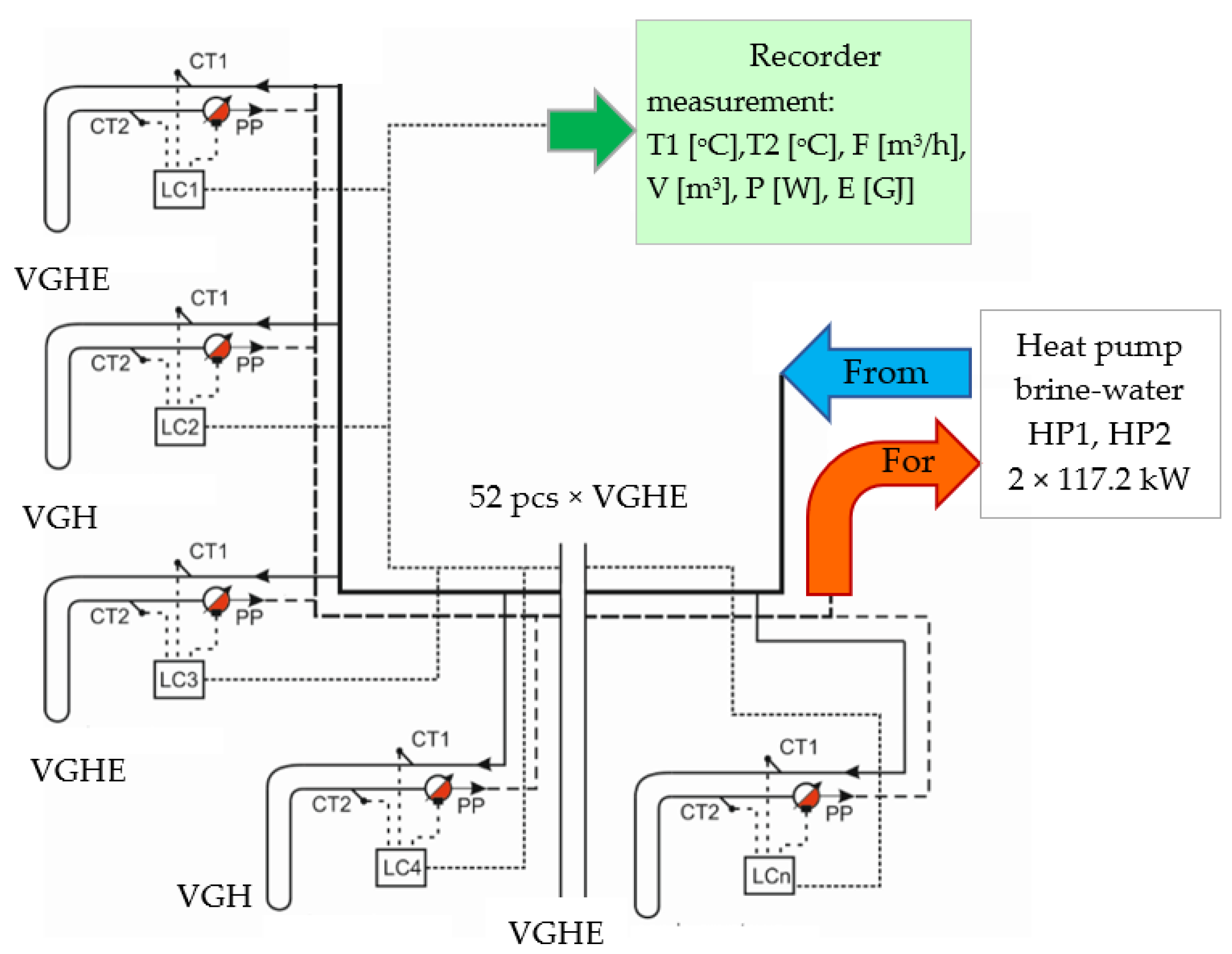
The system’s operation is controlled by a programmable heat pump controller with a heating curve directed towards a value of 1.0, enabling the achievement of a heating system temperature of +57 °C at an external temperature of −20 °C. The controller allows for the collaboration of heat pump cascades with a thermal node [2,5]. The system is metered, and all data are systematically collected, archived, and numerically displayed. Figure 2 illustrates the metering method.
In the analyzed period, the years 2018 and 2019, the heat pumps produced 446.55 MWh of heat energy, covering 100% of the heat demand without the need to activate the heat hub. The average annual coefficient of performance (COP) of the heat pumps, based on the energy balance, was 3.95. During the operation of the heating system, the brine temperature ranged from +0.2 to +10.7 °C, with an average value of +2.5 °C.

2.2. Selection of Variables for Model Construction

During the research conducted from January 2018 to December 2019, the following variables were recorded: C1—average outside air temperature °C, C2—heating season month, C3—average solar radiation intensity W/m2, C4—heating degree days °C·day, C5—energy consumption for heating the facility kWh, and d—brine supply temperature from the lower heat source (brine temperature) °C. Variables C1, C3, C5, and d were measured at a recording interval of 5 min.
Before proceeding to the main objective of this study, a pre-processing of the data was carried out by eliminating incomplete observations and aggregating the data to the corresponding periods, i.e., daily periods. As brine temperature is significantly influenced by tank capacity and regeneration time, the average brine flow rate dm3/day (described as C6) was recorded from the flow meter readings.
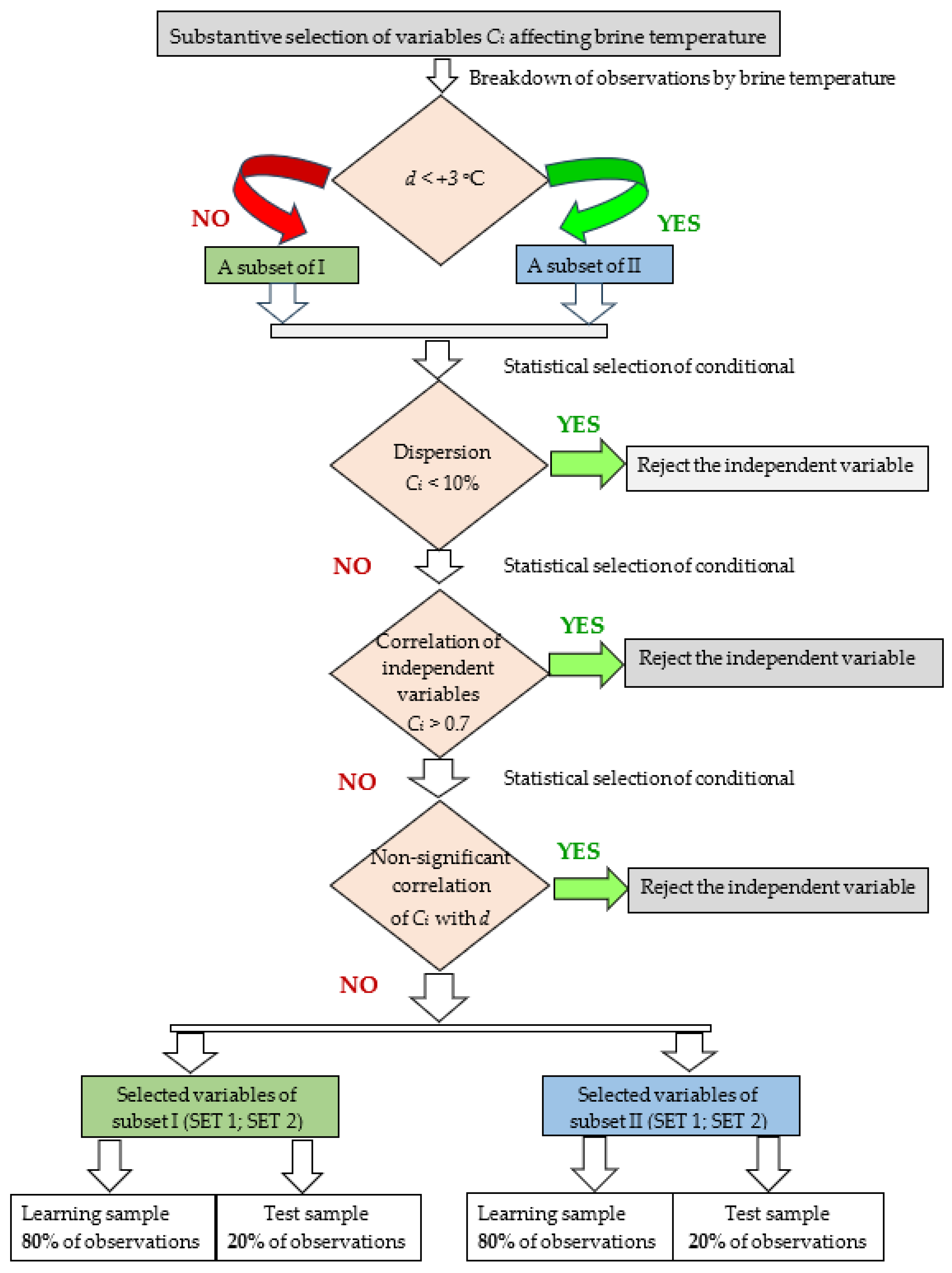
The statistical analysis performed indicated the existence of two subgroups of the community describing the influence of the independent variables on brine temperature. In the first step, the prepared data were divided into two subsets (subset I and subset II). The criterion for the division was brine temperature and +3 °C was taken as the cut-off value. Of the collected independent variables, only those were selected for which:
  • the coefficient of variation was greater than 10%;
  • the correlation coefficient between the independent variables was less than 0.7;
  • there was a statistically significant correlation between the dependent variable and the independent variable.
Next, two sets of independent variables (SET 1 and SET2) were each selected for subsets I and II. The first was built on meteorological and calendar data. The second set was extended by brine flow rate. In each subgroup, the observations were randomly divided into a learning subset and a test subset.
The detailed selection of variables is shown in Figure 3.

2.3. Construction and Quality Assessment of Forecasting Models

In the next step, from both subsets, observations were assigned to a learning group on which to build individual predictive and test models for their evaluation. From the first of these, 80% of the observations were drawn. For such prepared sets of variables, individual predictive models were developed [29,30,31,32,33,34,35,36,37].
  • ANNs—Artificial Neural Networks;
  • CARTs—Classification and Regression Trees;
  • CHAID—Chi-squared Automatic Interaction Detector;
  • FUZZY—Fuzzy Logic Toolbox;
  • MARSs—Multivariant Adaptive Regression Splines;
  • RTs—Regression Trees;
  • RST—Rough Set Theory;
  • SRTs—Support Regression Trees.
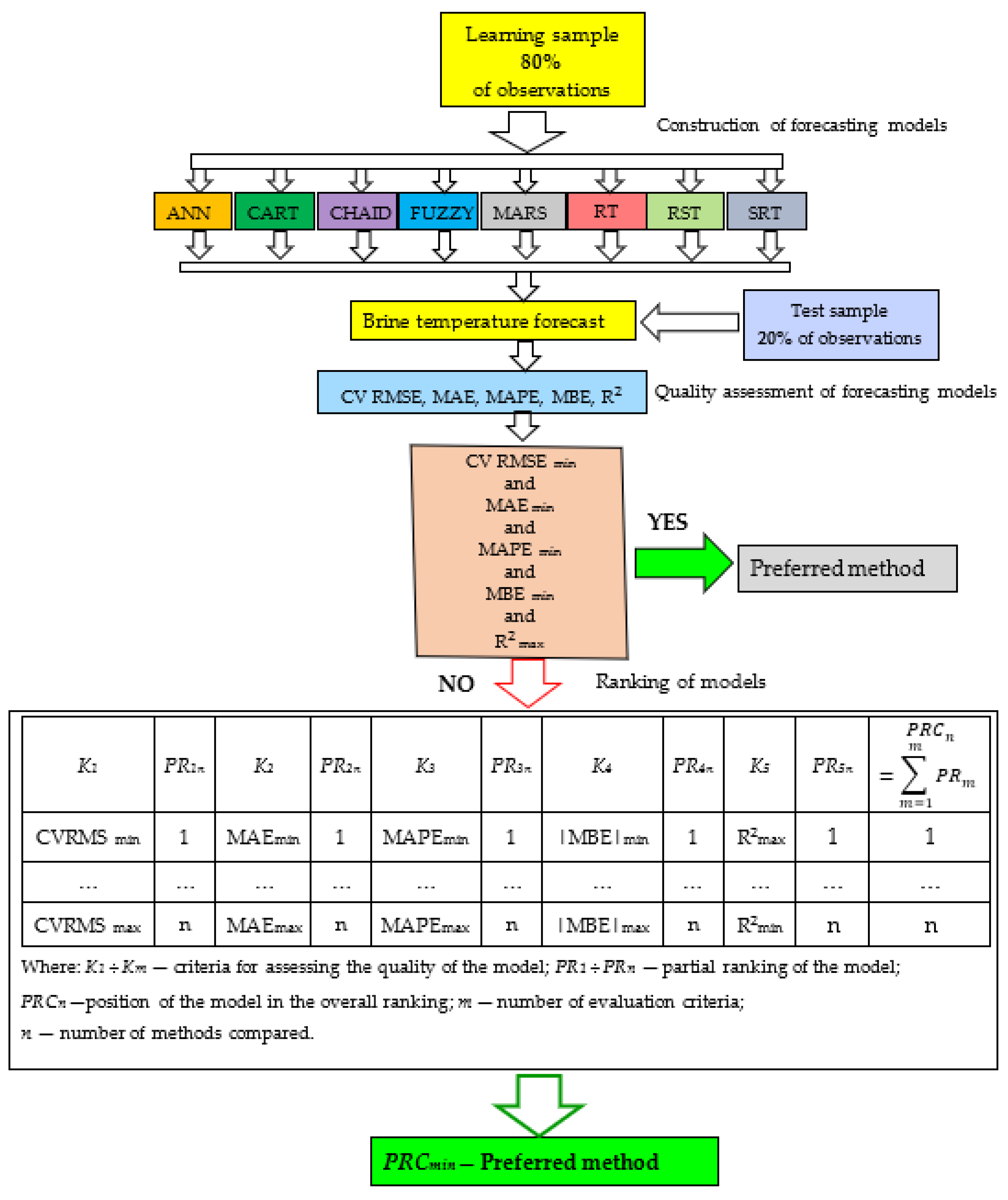
These models are included in the Matlab SIMULINK R2023b, StatSoft STATISTICA 13.1, and RSES2.1 software packages [38]. Their quality was evaluated according to the adopted methodology based on the following evaluation indicators: coefficient of variance of the root mean square error (CV RMSE), mean absolute error (MAE), mean absolute percentage error (MAPE), mean bias error (MBE), and coefficient of determination (R2), which are accepted as statistical calibration standards by ASHRAE Guideline 14-2014 [24,39,40]. The algorithm for the construction of the compared models and the method of assessing their quality is presented in Figure 4.

3. Discussion of Research Results

3.1. Preliminary Preparation of the Research Material

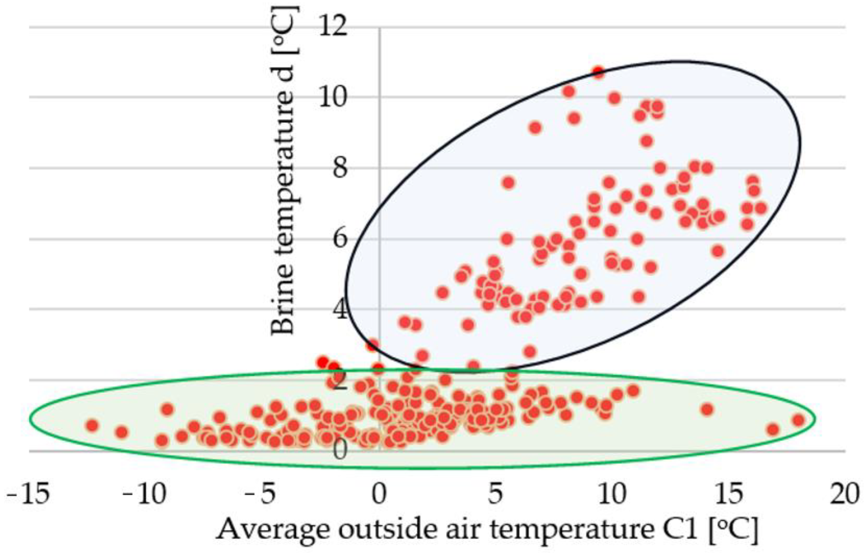
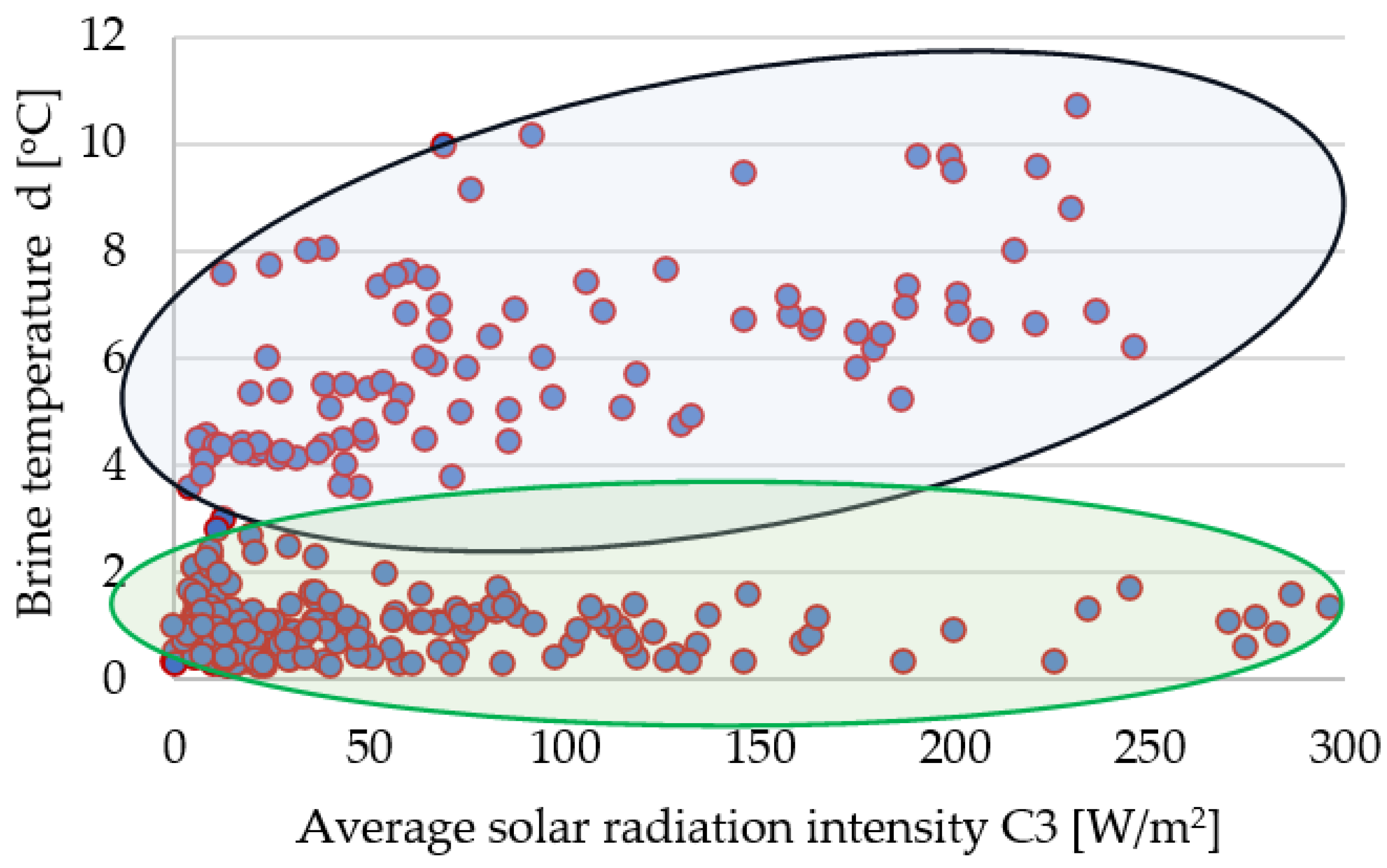
Before proceeding to the main objective of this study, the research material was pre-processed by eliminating incomplete observations and aggregating data. Graphical analysis of individual variables indicated that the collected research material was not homogeneous. The following figures show the effect of average outside air temperature (Figure 5) and solar radiation intensity on brine temperature (Figure 6).
In Figure 5 and Figure 6, two distinct series of brine temperature changes are visible. Therefore, the research material was divided into two subsets. The first subset was created for observations where the brine temperature was lower than +3 °C. This division allowed for a reduction of the variability of the decision variable (denoted as d) from over 100% to below 60% in subset I, and 30% in subset II. The characteristics of group I (ΔT < +3 °C) and group II (ΔT ≥ +3 °C) are presented in Table 1.
The next step was to select independent variables for modeling the brine temperature. To achieve this, correlation coefficients were calculated for the independent variables to eliminate strongly correlated variables. The analysis conducted (Table 2 and Table 3) indicates a very strong correlation between variables C1 and C4, as well as C1 and C5, and between C4 and C5. Therefore, in further analyses, variables C4 and C5 will not be taken into account.
To develop a forecast for the brine temperature, it is necessary to have knowledge of the independent variables with an appropriate lead time. In this study, an attempt was made to build two models (SET1 and SET2). SET1 utilizes variables such as average outside air temperature [°C] (C1), heating season month (C2), and average solar radiation intensity (C3). In SET2, the average brine flow rate dm3/day (C6) is additionally taken into account.

3.2. Assessing the Quality of Brine Temperature Prediction Models

For the prepared sets of variables, individual predictive models were developed, and their quality was assessed according to the adopted methodology (Figure 4). Since none of the examined methods exhibited the best indicators for all evaluation criteria simultaneously (Table 4—SET1, Table 5—SET2), a ranking of the compared models was then developed.
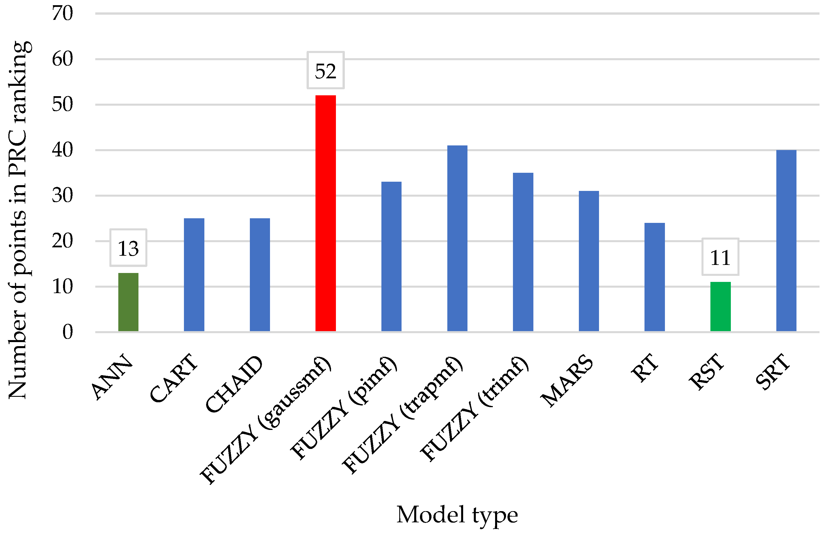
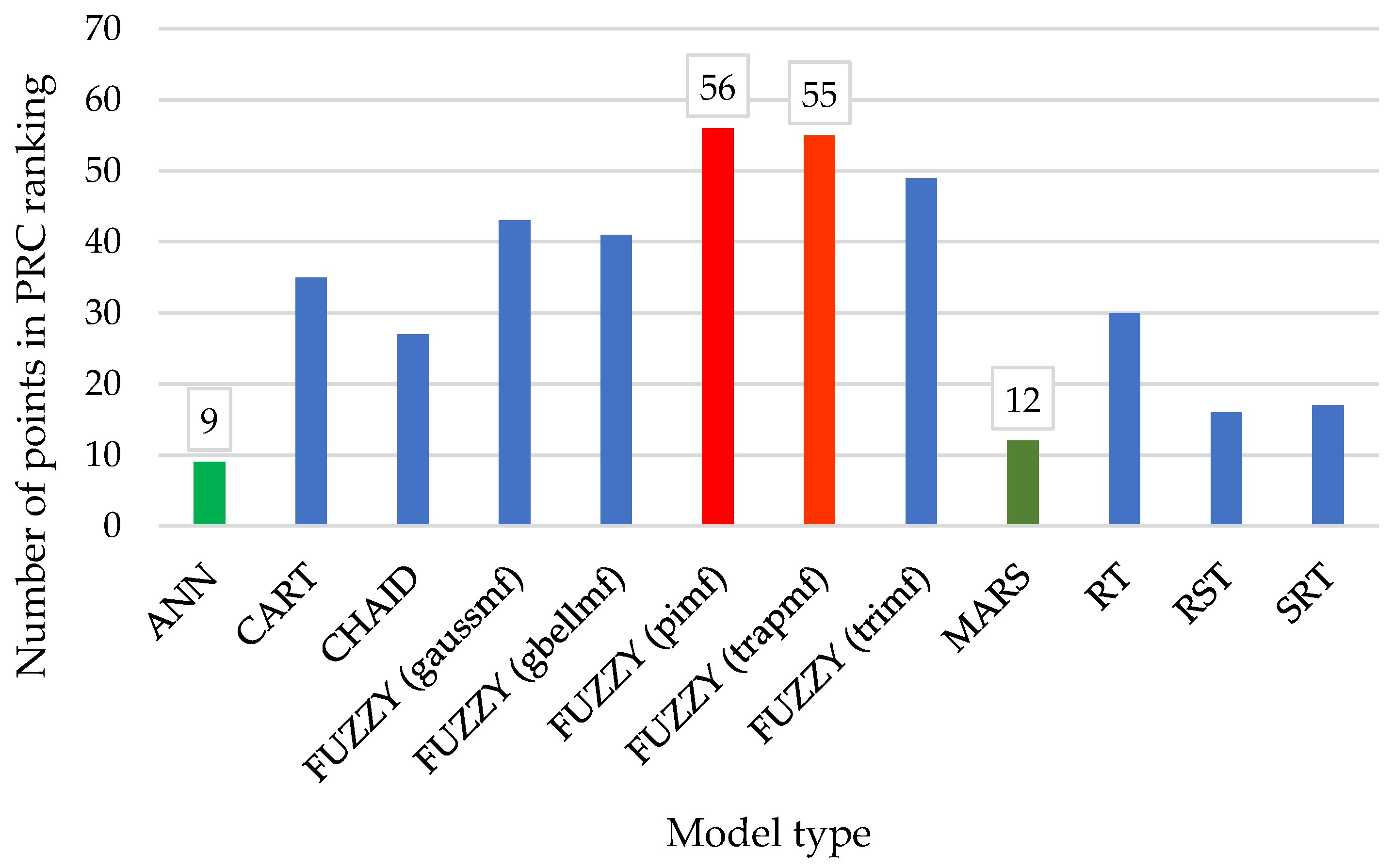
The evaluation process for each model was carried out by scoring the models on a scale of 1 to n, where 1 represents the best score and n represents the worst score for each evaluation criterion. Further evaluation criteria were the CV RMSE, MAE, MAPE, MBE, and R2. All of them, with the exception of R2, were treated as stimulants, i.e., the lower the value of the indicator the better the quality of the model. The evaluation did not vary the weights for the individual indicators describing the quality of the compared models. The sum of the scores from the individual evaluation criteria was then calculated for each model. In this way, an indicator describing the position of the model in the total ranking (PRC) was determined, taking into account all assessment criteria. The model with the lowest PRC value was considered to be the best model. In Figure 7, a comparison of the model quality of SET1 (three independent variables) is presented, while in Figure 8, the quality of the models of SET2 (four independent variables) is compared.
We can see that, when considering the independent variables from SET1, namely, average outside air temperature (C1), heating season month (C2), and average solar radiation intensity (C3), the highest quality forecasts were obtained for the Rough Set Theory (RST) and Artificial Neural Network (ANN). The best among the compared methods (RST) exhibited partial evaluation indicators of CV RMSE 21.56%, MAE 0.3 °C, MAPE 14.3%, and R2 96%. The second group consisted of regression tree models (CART, CHAID, and RT), which allowed for predictions with errors at the level of CV RMSE 25 to 30%, MAE around 0.4 °C, MAPE 20 to 22%, MBE −4.4 to −0.13, and R2 91 to 94%. The remaining models generated forecasts with higher errors. For the second set of variables (SET2), expanded with information describing the average brine flow rate (C6), the best methods could be considered the Artificial Neural Networks and the Multivariate Adaptive Regression Splines (MARSs) methods. They generated forecasts with errors ranging from 3.7 to 4.6% for CV RMSE, up to 0.06 °C for MAE, 2 to 5% for MAPE, up to 1% for MBE, and R2 was close to 100%. Slightly lower-quality forecasts were obtained for the models using Rough Set Theory (RST) and Boosted Regression Trees (SRTs). The errors of these models did not exceed 15% for CV RMSE, 0.2 °C for MAE, 10% for MAPE, and −0.2% for MBE, and R2 oscillated around 0.98.

4. Summary and Conclusions

The temperature of the brine has a decisive impact on the efficiency and durability of heat pump systems that use ground heat exchangers of the brine water type. Extended operation of heat pumps at excessively low brine temperatures results in a substantial reduction in the ground temperature surrounding the heat exchanger pipes. This, in turn, impacts the duration of the ground regeneration process and elevates the number of freezing and thawing cycles for the material filling the borehole. Such unstable operating conditions of a ground heat exchanger can, in extreme cases, lead to mechanical damage to the heat exchanger tubes caused by expanding ice. In the absence of the full thermal regeneration of the ground in subsequent heating seasons, it will not provide the ground with the appropriate amount of heat. As a result of the reduced capacity of the lower heat source, there may be an emergency shutdown of heat pumps during their operation, which, in turn, will affect the energy efficiency and durability of the system. Therefore, monitoring and forecasting the temperature of the brine becomes a key element in maintaining the high efficiency of the system. Accurate forecasting of this parameter is particularly important in conditions of variable external temperatures.
This article presents a comparison of selected methods for forecasting the temperature of brine using either artificial neural networks, classification and regression trees, or the theory of approximate sets. Of practical value to readers is the information on which method can be used, depending on the input data available to the researcher, to obtain the best results and fit. Based on the comparative analysis of various methods used for forecasting the temperature of brine, it can be seen that the choice of the preferred method depends on the available data. This allows for a flexible approach to forecasting. It has been shown that, even with a limited number of independent variables, it is possible to obtain results with an acceptable error. This research not only sheds light on the issue of forecasting the temperature of brine but also opens up new possibilities for the practical application of the indicated methods in monitoring and controlling the operation of heat pump systems. The developed algorithms of the indicated methods can be programmed, and their results can be used to control the operation of the heating system in the object.
For the studied object, a comparative analysis of eight methods for forecasting the temperature of the brine from vertical ground heat exchangers was carried out based on real data. The results obtained made it possible to identify the best predictive methods depending on the number and type of independent variables. The conclusions of the analysis are as follows:
  • From the comparative evaluation of selected models forecasting the brine temperature from vertical ground heat exchangers (VGHEs), it is evident that for a limited set of variables using readily available weather data, such as the average daily outside air temperature, the month of the heating season, and the average solar radiation intensity, the best quality forecasts were obtained using the method based on Rough Set Theory (RST). An alternative method could be Artificial Neural Networks (ANNs), which allow for predictions with slightly higher errors.
  • For a larger number of independent variables (such as the average daily outside air temperature, the month of the heating season, average solar radiation intensity, and the amount of brine flowing through the ground heat exchangers), the use of Artificial Neural Networks (ANNs) and the Multivariate Adaptive Regression Splines (MARSs) method are preferred.
  • The conducted research confirmed the influence of meteorological conditions on brine temperature and, consequently, the temperature of the geothermal reservoir. Two different trends in the influence of external temperature and solar radiation intensity on brine temperature were observed. The research indicated a difference at the level of +3 °C.

Author Contributions

Conceptualization J.P.-W. and T.S., data curation J.P.-W.; investigation J.P.-W., T.S., K.N. and S.L., methodology J.P.-W., T.S. and K.N., project administration J.P.-W. and T.S., supervision J.P.-W. and T.S.; writing—original draft J.P.-W., T.S., K.N. and S.L.; writing—reviewing and editing J.P.-W., T.S., K.N. and S.L. All authors have read and agreed to the published version of the manuscript.

Funding

This work was performed within the framework of grants from the Bialystok University of Technology (WZ/WBiIS/6/2023) and the APC is financed by the University of Agriculture in Krakow.

Data Availability Statement

The data presented in this study are available on request from the corresponding author.

Conflicts of Interest

The author declares no conflicts of interest.

References

  1. Rybach, L.; Sanner, B. Ground-source heat pump systems the European experience. GHC Bull. 2000, 21, 16–26, ISSN 0276-1084. [Google Scholar]
  2. Piotrowska-Woroniak, J. Assessment of Ground Regeneration around Borehole Heat Exchangers between Heating Seasons in Cold Climates: A Case Study in Bialystok (NE, Poland). Energies 2021, 14, 4793. [Google Scholar] [CrossRef]
  3. Zhao, Y.; Pang, Z.; Huang, Y.; Ma, Z. An efficient hybrid model for thermal analysis of deep borehole heat exchangers. Geotherm. Energy 2020, 8, 18. [Google Scholar] [CrossRef]
  4. Kasuda, T.; Archenbach, P. Earth temperature and thermal diffusivity at selected stations in the United States. Ashrae Trans. 1965, 71, 61. [Google Scholar] [CrossRef]
  5. Piotrowska—Woroniak, J. Preliminary results of the temperature distribution measurements around the vertical ground heat exchangers tubes. Ecol. Chem. Eng. S 2020, 27, 509–528. [Google Scholar] [CrossRef]
  6. Rad, F.M.; Fung, A.S.; Leong, W.H. Feasibility of combined solar thermal and ground source heat pump systems in cold climate, Canada. Energy Build. 2013, 61, 224–232. [Google Scholar] [CrossRef]
  7. Saskia, M.M.; Wallin, E. Ground temperature profiles and thermal rock properties at Wairakei, New Zealand. Renew. Energy 2012, 43, 313–321. [Google Scholar] [CrossRef]
  8. Rad, F.M.; Fung, A.S. Solar community heating and cooling system with borehole thermal energy storage—Review of systems. Renew. Sustain. Energy Rev. 2016, 60, 1550–1561. [Google Scholar] [CrossRef]
  9. Spitler, J.D.; Gehlin, S.E. Thermal response testing for ground source heat pump systems-An historical review. Renew. Sustain. Energy Rev. 2015, 50, 1125–1137. [Google Scholar] [CrossRef]
  10. Al—Temeemi, A.; Harris, D. The generation of subsurface temperature profiles for Kuwait. Energy Build. 2001, 33, 837–841. [Google Scholar] [CrossRef]
  11. Spitler, J.; Bernier, M. 2-Vertical borehole ground heat exchanger design methods. In Advances in Ground-Source Heat Pump Systems; Rees, S.J., Ed.; Woodhead Publishing: Oxford, UK, 2016; pp. 29–61. ISBN 978-0-08-100311-4. [Google Scholar] [CrossRef]
  12. Naicker, S.S.; Rees, S.J. Long-term high frequency monitoring of a large borehole heat exchanger array. Renew. Energy 2020, 145, 1528–1542. [Google Scholar] [CrossRef]
  13. Nian, Y.; Cheng, W. Analytical g-function for vertical geothermal boreholes with effect of borehole heat capacity. Appl. Therm. Eng. 2018, 140, 733–744. [Google Scholar] [CrossRef]
  14. Yu, X.; Li, H.; Yao, S.; Nielsen, V.; Heller, A. Development of an efficient numerical model and analysis of heat transfer performance for borehole heat exchanger. Renew. Energy 2020, 152, 189–197. [Google Scholar] [CrossRef]
  15. Ghoreish-Madiseh, S.; Kuyuk, A.; de Brito, M.A.R. An analytical model for transient heat transfer in ground-coupled heat exchangers of closed-loop geothermal systems. Appl. Therm. Eng. 2019, 150, 696–705. [Google Scholar] [CrossRef]
  16. Kerme, E.D.; Fung, A.S. Heat transfer simulation, analysis and performance study of single U-tube borehole heat exchanger. Renew. Energy. 2020, 145, 1430–1448. [Google Scholar] [CrossRef]
  17. Sailer, E.; Taborda, D.M.G.; Zdravković, L. A new approach to estimating temperature fields around a group of vertical ground heat exchangers in two-dimensional analyses. Renew. Energy 2018, 118, 579e590. [Google Scholar] [CrossRef]
  18. Pan, A.; Lu, L.; Tian, Y. A new analytical model for short vertical ground heat exchangers with Neumann and Robin boundary conditions on ground surface. Int. J. Therm. Sci. 2020, 152, 106326. [Google Scholar] [CrossRef]
  19. Boban, L.; Soldo, V.; Fuji, H. Investigation of heat pump performance in heterogeneous ground. Energy Convers. Manag. 2020, 211, 112736. [Google Scholar] [CrossRef]
  20. Port, P.C. Guidelines for Designing, Realization and Receiving Installations Powered by Heat Pumps; Part 1; Polish Organization for the Development of Heat Pump Technology: Cracow, Poland, 2013. (In Polish) [Google Scholar]
  21. Vella, C.; Borg, S.P.; Micallef, D. The Effect of Shank-Space on the Thermal Performance of Shallow Vertical U-Tube Ground Heat Exchangers. Energies 2020, 13, 602. [Google Scholar] [CrossRef]
  22. Bakirci, K. Evaluation of the performance of a ground-source heat-pump system with series GHE (ground heat exchanger) in the cold climate region. Energy 2010, 35, 3088–3096. [Google Scholar] [CrossRef]
  23. Piotrowska-Woroniak, J.; Szul, T.; Woroniak, G. Application of a Model Based on Rough Set Theory (RST) for Estimating the Temperature of Brine from Vertical Ground Heat Exchangers (VGHE) Operated with a Heat Pump—A Case Study. Energies 2023, 16, 7182. [Google Scholar] [CrossRef]
  24. ASHRAE. American Society of Heating, Ventilating, and Air Conditioning Engineers (ASHRAE), Guideline 14-2014, Measurement of Energy and Demand Savings; Technical Report; American Society of Heating, Ventilating, and Air Conditioning Engineers: Atlanta, GA, USA, 2014; Available online: https://upgreengrade.ir/admin_panel/assets/images/books/ASHRAE%20Guideline%2014-2014.pdf (accessed on 5 November 2023).
  25. ANSI/ASHRAE Standard 169-2021; Climatic Data for Building Design Standards. American Society of Heating. Refrigerating and Air-Conditioning Engineers: Atlanta, GA, USA, 2021.
  26. Peel, M.C.; Finlayson, B.L.; McMahon, T.A. Updated world map of the Köppen-Geiger climate classification. Hydrol. Earth Syst. Sci. 2007, 11, 1633–1644. [Google Scholar] [CrossRef]
  27. Institute of Meteorology and Water Management. Data from the Institute of Meteorology and Water Management. Available online: https://meteo.imgw.pl/ (accessed on 18 March 2023). (In Polish).
  28. Piotrowska-Woroniak, J. Determination of the Selected Wells Operational Power with Borehole Heat Exchangers Operating in Real Conditions, Based on Experimental Tests. Energies 2021, 14, 2512. [Google Scholar] [CrossRef]
  29. Song, Q.; Chissom, B.S. Fuzzy time series and its models. Fuzzy Sets Syst. 1993, 54, 269–277. [Google Scholar] [CrossRef]
  30. Pawlak, Z. Rough Sets. Theoretical Aspects of Reasoning about Data; Kluwer Academic Press: Dordrecht, The Netherlands, 2012; Available online: http://bcpw.bg.pw.edu.pl/Content/2026/RoughSetsRep29.pdf (accessed on 1 November 2023).
  31. Nebot, A.; Mugica, F. Energy Performance Forecasting of Residential Buildings Using Fuzzy Approaches; Applied Sciences: Basel, Switzerland, 2020. [Google Scholar]
  32. Mathworks. Membership Function Gallery. Available online: https://www.mathworks.com/help/fuzzy/membership-function-gallery.html (accessed on 5 November 2023).
  33. Nauck, D.; Klawonn, F.; Kruse, R. Neuro-Fuzzy Systems; John Wiley & Sons: Hoboken, NJ, USA, 1997. [Google Scholar]
  34. Rendon-Sanchez, J.F.; Menezes, L.M. Structural combination of seasonal exponential smoothing forecasts applied to load forecasting. Eur. J. Oper. Res. 2019, 275, 916–924. [Google Scholar] [CrossRef]
  35. Eynard, J.; Grieu, S.; Polit, M. Wavelet-based multi-resolution analysis and artificial neural networks for forecasting temperature and thermal power consumption. Eng. Appl. Artif. Intell. 2010, 24, 501–516. [Google Scholar] [CrossRef]
  36. Friedman, J. Multivariate adaptive regression splines (with discussion). Ann. Stat. 1991, 19, 1–141. [Google Scholar]
  37. Hastie, T.; Tibshirani, R.; Friedman, J.H. The Elements of Statistical Learning: Data Mining, Inference, and Prediction; Springer: New York, NY, USA, 2001. [Google Scholar]
  38. Rough Set Exploration System 2.1. Available online: https://www.mimuw.edu.pl/~szczuka/rses/start.html (accessed on 15 November 2023).
  39. Ruiz, G.R.; Bandera, C.R. Validation of Calibrated Energy Models: Common Errors. Energies 2017, 10, 1587. [Google Scholar] [CrossRef]
  40. Szul, T. Application of a Thermal Performance-Based Model to Prediction Energy Consumption for Heating of Single-Family Residential Buildings. Energies 2022, 15, 362. [Google Scholar] [CrossRef]
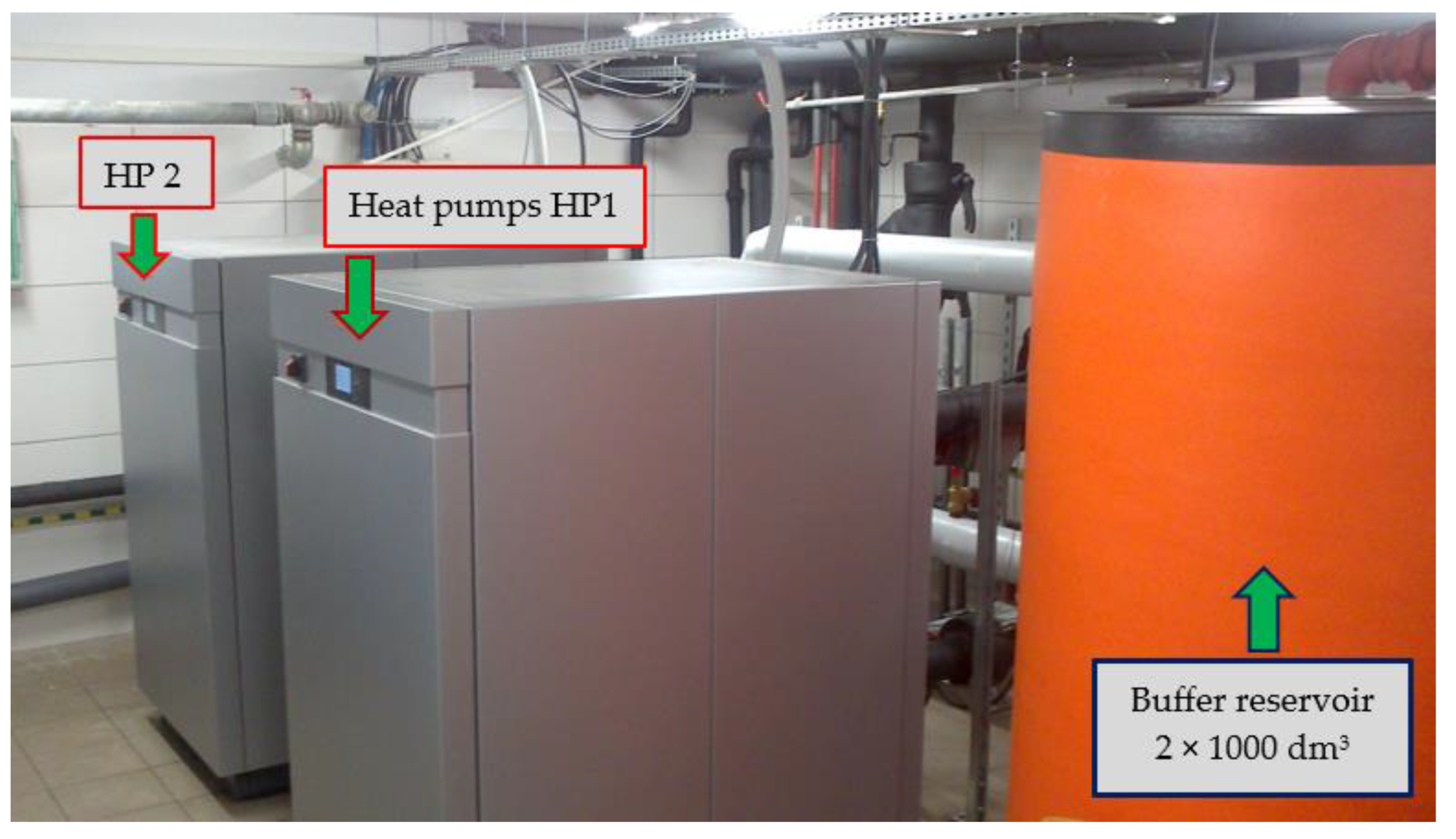
Figure 1. Two heat pumps, brine water type heating, power 117.2 kW, and buffer tanks with a capacity of 1000 dm3 (photography author).
Energies 17 01465 g001
Figure 2. Metering of ground vertical probes (VGHEs), designations: PP—flow transducer; CT1, CT2—temperature sensors; LCn—microprocessor-based conversion system; T1, T2—temperature °C; F—brine flow m3/h; V—brine volume m3; E—energy extracted from the ground GJ.
Energies 17 01465 g002
Figure 3. Algorithm for selecting independent variables for modeling brine temperature.
Energies 17 01465 g003
Figure 4. Algorithm for building and evaluating a predictive model.
Energies 17 01465 g004
Figure 5. Effect of average outside air temperature (C1) on brine temperature (d).
Energies 17 01465 g005
Figure 6. Effect of average solar radiation intensity (C3) on brine temperature (d).
Energies 17 01465 g006
Figure 7. Aggregate assessment of model quality for three independent variables (SET1: C1, C2, C3).
Energies 17 01465 g007
Figure 8. Aggregate assessment of model quality for four independent variables (SET2: C1, C2, C3, C6).
Energies 17 01465 g008
Table 1. Characteristics of variability of subsets I and II.
VariableSubset ISubset II
AverageMinMaxCoefficient
of Variation
AverageMinMaxCoefficient
of Variation
C11.18−12.3217.93384.139.111.1116.3839.34
C241.009.0079.637.286.008.009.67
C348.450.00296.15125.5690.554.13246.1578.18
C417.130.3730.6226.479.191.9517.1938.99
C52141.4246.713838.9626.001150.33241.002138.2539.01
C63372.2454.9512,736.5679.78219.6035.29592.3159.13
d0.960.242.9856.316.053.5610.7128.98
Table 2. Correlation coefficients for subset I.
VariableC1C2C3C4C5C6d
C11.00
C20.011.00
C30.431.001.00
C4−1.00−0.01 *−0.431.00
C5−1.00−0.03 *−0.431.001.00
C6−0.67−0.46−0.130.670.671.00
d0.360.57−0.01 *−0.36−0.36−0.751.00
*—correlation not statistically significant.
Table 3. Correlation coefficients for subset II.
VariableC1C2C3C4C5C6d
C11.00
C2−0.441.00
C30.50−0.481.00
C4−1.000.44−0.501.00
C5−1.000.43−0.511.001.00
C6−0.620.57−0.590.920.921.00
d0.57−0.600.58−0.57−0.57−0.791.00
Table 4. Quality assessment of models for three conditional attributes (SET1).
No.MethodCV RMSE
%
MAE
°C
MAPE
%
MBE
%
R2
-
1ANN25.310.3318.29−0.680.94
2CART30.630.420.58−0.130.91
3CHAID30.120.420.24−0.440.91
4FUZZYpimf38.160.4320.321.250.86
trimf38.540.4319.621.510.86
trapmf39.560.4427.630.070.85
gaussmf83.780.6122.878.260.47
5MARS26.380.4125.54−3.320.93
6RT24.820.3721.89−4.390.94
7RST21.560.2814.33.090.96
8SRT28.90.4825.87−6.850.93
Table 5. Quality assessment of models for four conditional attributes (SET2).
No.MethodCV RMSE
%
MAE
°C
MAPE
%
MBE
%
R2
-
1ANN4.610.051.670.390.99
2CART18.950.2711.89−4.060.97
3CHAID16.540.2412.39−1.70.98
4FUZZYgaussmf27.830.2816.633.250.93
gbellmf40.260.3613.840.360.86
pimf49.760.4416.269.420.77
trapmf49.660.3913.9710.160.77
trimf31.990.3420.855.50.91
5MARS3.70.064.551.080.99
6RT17.150.2510.28−1.550.97
7RST15.330.28.57−0.170.98
8SRT14.50.229.87−0.110.98
Disclaimer/Publisher’s Note: The statements, opinions and data contained in all publications are solely those of the individual author(s) and contributor(s) and not of MDPI and/or the editor(s). MDPI and/or the editor(s) disclaim responsibility for any injury to people or property resulting from any ideas, methods, instructions or products referred to in the content.