Abstract
The mass introduction of renewable energy sources (RESs) presents numerous challenges for transmission system operators (TSOs). The Italian TSO, Terna S.p.A., aims to assess the impact of inverter-based generation on system inertia, primary regulating energy and short-circuit power for the year 2030, characterized by a large penetration of these sources. The initial working point of the Italian transmission network has to be defined through load flow (LF) calculations before starting dynamical analyses and simulations of the power system. Terna 2030 development plan projections enable the estimation of active power generation and load for each hour of that year in each Italian market zone, as well as cross-zonal active power flows; this dataset differs from conventional LF assignments. Therefore, in order to set up a LF analysis for the characterization of the working point of the Italian transmission network, LF assignments have to be derived from the input dataset provided by Terna. For this purpose, this paper presents two methods for determining canonical LF assignments for each network bus, aligning with the available data. The methodologies are applied to a simplified model of the Italian network, but they are also valid for other transmission networks with similar topology and meet the future needs of TSOs. The methods are tested at selected hours, revealing that both approaches yield satisfactory results in terms of compliance with the hourly data provided.
1. Introduction
Electric networks are moving toward a higher level of complexity. The integration of an increasingly large portion of renewable energy sources (RESs), such as wind turbines (WTs) and photovoltaic (PV) units [1,2], and of battery energy storage systems (BESSs) into the traditional electric system [3], either in place of or in addition to conventional synchronous generators (SGs) (e.g., thermoelectric and hydroelectric ones), presents a significant challenge for the system in terms of safety and resiliency, also taking into account the growing installation of inverter-based loads and of high voltage direct current (HVDC) links [4]. The main effects of RES penetration are a decrease in system short-circuit power, in physical inertia and in primary regulating energy, possibly causing issues associated with voltage and frequency instability [5,6,7] and power quality issues (see, e.g., Refs. [8,9]). Therefore, transmission system operators (TSOs) require RESs to act like traditional power plants and play an important role in voltage and frequency stability enhancement, withstanding various disturbances and improving the power quality, reliability and security of the electrical grid, as reported in refs. [10,11]. Focusing on frequency stability, TSOs have begun implementing a number of frequency support (FS) actions to address this issue, including the installation of synchronous compensators (SCs) and the introduction of advanced control functionalities for inverter-based generation, which are able to provide the FS services required by the network [12,13]. Moreover, RES can support local voltage stability and short-term voltage stability thanks to the implementation of specific control techniques, as described in refs. [14,15].
In this scenario, the knowledge of pre-perturbation conditions is fundamental to studying the transient and the impact of the actions provided by RESs in response to severe perturbations. Load flow (LF) analysis provides a comprehensive understanding of the steady-state behavior of power systems by quantifying the voltages, currents and power flows at various nodes and branches. Therefore, LF serves as a fundamental tool for system planning, design and operation, allowing engineers to study voltage and frequency stability problems [16].
The LF problem determines the amplitudes and phases of voltages at the nodes of a network under steady-state conditions, after fixing the correct number of assignments and using active and reactive power balance equations reported in ref. [17]. Since the resulting equations are non-linear, numerical iterative methods are implemented to produce a solution, which is within a reasonable tolerance [18].
Assignments in LF analysis refer to the allocation of loads, generation sources and network parameters to specific components within the power system. Proper LF assignments are essential for accurate modeling of the system, as they determine the distribution and utilization of power across the network. Incorrect or imprecise LF assignments may lead to inaccurate power flow calculations, resulting in voltage violations, excessive losses and inefficient utilization of network resources [19].
These assignments involve specifying the active and reactive power demands at load nodes, the generation’s production and characteristics at generator nodes and the impedance and admittance values of transmission lines and transformers.
LF assignments consist of sets of two mathematical assignments for each bus: at load buses, also named PQ buses, the active power and reactive power absorptions are assigned; at generation buses, also called PV buses, the injected active power and voltage magnitude are defined; finally, at the so-called slack buses, the voltage amplitude and voltage phase are arbitrarily assigned, so that these buses act as independent voltage sources. Slack buses are defined in order to close complex power balances because it is not possible to assign the real power injected at all the network nodes (losses are, in principle, unknown, as they depend on the currents, which are an output of the problem) [20].
However, it is not always easy to know the required assignments of the LF analysis because, sometimes, they are not deterministic or because, in some cases, the available data are not usual. Considering the variability in RES production, the probabilistic approaches for evaluating LF, which take into account the unpredictability of nodal data, are described in multiple studies [21,22,23].
The literature, on the other hand, is not very well supplied with studies, which consider unusual load flow assignments. Optimal power flow (OPF) problems are focused on the optimization of operations of a power system; their objective is to minimize the total cost of electricity generation while granting the safe operations of the power system. These techniques are therefore an extension of economic dispatching problems, also taking into account LF equations. OPF problems differ from the problem highlighted in the present manuscript because their aim is the optimal dispatching of generators’ production. Power system state estimation (PSSE) techniques—proposed in several papers, among which, Ref. [24]—are methodologies aimed at finding more accurate voltage magnitudes and angles at the buses of a system in which observed measurements are available. Nevertheless, those measurements also involve voltage magnitudes at certain buses and reactive power flows, together with an estimation of measurement errors characterizing measurement devices. Another study, presented in Ref. [25], deals with the lack of measurements (due to communication systems’ interruptions, for example), leading to a data recording, which is inconsistent for performance of a PSSE analysis. Nevertheless, in the case under consideration in this manuscript, the Italian TSO, Terna S.p.A. (from now on, “Terna”), provided the authors with a set of data, which are not derived from a measurement campaign but from day-ahead market simulations, not taking into account directly possible forecasting mistakes and obviously not being affected by measurement inconsistencies.
On the one hand, Terna needs to perform some dynamical analyses to check the impact of the future generation mix on the aforementioned issues (inertia, primary regulating energy, reactive power and short-circuit power), such as the ones presented in Refs. [26,27]; however, on the other hand, Terna prepared a 2030 development plan, which allows an estimation of the generation and load active power in each Italian market zone and the cross-zonal active power flows. As a result, the nodes of the Italian transmission network do not belong to any of the aforementioned bus categories.
Therefore, the paper proposes two methods of finding a set of LF assignments compliant with the data provided by the TSO. The first method, called the “optimization method”, sets up a non-linear optimization problem, while the second one, called the “analytical method” and based on the structure of the Italian transmission grid, does not use any numerical method. No other examples of similar studies were found in the literature. The present study proposes two methods, which are applied to the Italian transmission network, fully developed in agreement with and under the supervision of the Italian TSO, ensuring the coherence between the forecasted data provided by Terna, which they are used to handling, and the missing data, which are essential for the development of further analyses, such as LF and dynamical analyses.
The present paper is organized as follows. Section 2 provides a detailed description of the dataset relevant to the 2030 scenario, providing a brief overview of the methodology followed by Terna to obtain it, a presentation of the model of the Italian network and a detailed formalization of the two methods developed to estimate the necessary LF assignments, being compliant with the available data. Section 3 shows the comparison between the results of the optimization and analytical methods. Finally, Section 4 presents concluding remarks.
2. Materials and Methods
This section first presents the dataset relevant to the 2030 scenario, together with the assumptions made and the methodology followed by Terna to obtain them. Having pointed out the lack of necessary data for setting up a LF analysis for the characterization of the Italian transmission network working point within the dataset provided, two methods for the definition of the LF assignments required, consistent with the data provided by Terna, are thoroughly analyzed and discussed.
2.1. Dataset Description
The Italian transmission network scenario is characterized by Terna for the year 2030, following a detailed forecasting approach described in Ref. [28]. Exploiting the historical series of load profiles, modified according to the future penetration of new type of electric loads (electric vehicles, heat pumps, etc.), hourly load profiles are determined for each market zone and for each hour in the year 2030. Terna developed an algorithm running for each hour of the year—a simulation of the day-ahead market (DAM) session—in order to define the generation, which will be “in the market”, satisfying the demand, the active power flows in Italian cross-zonal lines and in lines between Italy and neighboring foreign countries while taking into account the possible compulsoriness of dispatchment services (satisfaction of power reserve constraints and resolution of congestions).
For each hour of the year 2030 and for each Italian market zone (a market zone is a portion of the network for which limitations of power exchange with neighboring market zones exist; these limitations are imposed in order to grant safe operations of the transmission system. Market zones play an important role in the electricity market; purchase and sale offers are accepted only if the power exchange capacity between market zones is not overcome) i (i = 1 … N) [29], the data characterizing the future scenario consist of the overall active power generation PG,i, the overall active power demand PL,i and the active power flows in AC and HVDC lines. The parameters of each cross-zonal AC or HVDC line are also provided.
As specified in the Introduction, the 2030 scenario described above is used to perform some perspective analyses to infer possible critical issues and to define proper countermeasures. Among them, it is worth citing
- simulations looking for possible frequency instability and obtaining an insight on the future transmission network inertia needs (to be satisfied either by new synchronous generator or compensator installations or by the provision of synthetic inertia by BESS or RES);
- short-circuit analysis to check whether the mass introduction of converter-based generation will result in an unacceptable reduction in short-circuit power.
Such dynamical analyses are usually carried out by exploiting a dedicated software (e.g., DIgSILENT PowerFactory 2022), which requires an initial working point in order to start the transient simulation. As is well known, in power systems, a working point is defined once the solution of a LF calculation is available. However, the dataset described above does not contain all the data, which would be needed in order to set up a LF calculation, because (i) the active power injection at each node is not sufficient for characterizing it in any of the three classical categories (load bus, generation bus and slack bus), and (ii) active power flows in the network branches are normally an output of the LF calculation. In fact, Terna did not forecast and did not provide the authors with information regarding the reactive power injection in each market zone (likewise, no information was provided regarding voltage amplitude, which would be meaningless, since we are dealing with market zones composed of several physical nodes), preventing the possibility of launching a LF calculation; in fact, in order to be performed, a LF calculation requires either one of the two aforementioned (conventional) assignments in order to characterize a bus as a PQ bus or a PV bus.
For this reason, two methods are developed in order to find a set of LF assignments (active power injection and voltage amplitude at each node) compliant with the data provided by Terna.
All the countries neighboring Italy at the northern border (France, Switzerland, Austria and Slovenia) are grouped as an equivalent node called “node 1”. Terna provides the parameters of each cross-zonal connection from which the parameters of the equivalent link between node 1 and the Italian node “north” can be derived. The Italian market zones along the peninsula are numbered from 2 to 7, and Malta is defined as “node 8” because, despite being a foreign node, it is needed in order to close the balances.
All HVDC power flows are considered as simple power injections at the Italian terminal market zones; for this reason, the Italian market zone “Sardegna” and foreign market zones “Corsica”, “Montenegro”, “Greece” and “Tunisia” are not included in the simplified model of the Italian network, but the flows between these zones and Italian market zones are codified as power injections. Therefore, the active power injected at the i-th node is obtained from the active power balance applied to node i:
where is the net HVDC power injection at node i.
According to these assumptions, a simplified model of the Italian transmission network is developed in agreement with Terna and its guidelines; this model, represented as shown in Figure 1, exploits the subdivision of the Italian transmission network into market zones, as ruled by the TSO. AC lines are represented in blue, while HVDC links are represented in red. The Italian territory is depicted in dark gray, whilst foreigner countries are represented in light gray. The eight nodes considered for LF analysis are highlighted in blue, while nodes, which are not directly involved in the analysis, are highlighted in red.
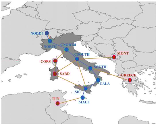
Figure 1.
Simplified scheme of the Italian network. The Italian territory is depicted in dark gray, whilst foreigner countries are represented in light gray.
The proposed model configuration was validated by Terna, being compliant with the structure of the data provided in the received dataset.
2.2. Methods
This subsection presents a detailed description of the two methods. Starting from the dataset provided by Terna (active power injections at each node and active power flows in each interconnection line), the aim of both methods is to determine conventional LF assignments (e.g., active and reactive power injection or active power injection and voltage magnitude at each node, except for the slack one) in order to set up a LF calculation. The active power flows found as a result of the LF calculation should be as close as possible to the ones provided by Terna. The first method, called the “optimization method”, sets up a non-linear optimization problem, while the second one, called the “analytical method”—exploiting the peculiar structure of the network in Figure 1—does not rely on any numerical method.
2.2.1. Optimization Method
The first approach consists of transforming the LF problem into an optimization problem, which allows us to obtain the value of voltage amplitude at each node of the network while satisfying a set of constraints. These constraints are associated with the active power injections at each node. The objective function is defined in order to minimize the deviation in nodal voltage amplitudes from their rated values (one per unit in the Italian transmission network voltage base being rated) and the deviation in active power flows from the data provided by Terna, called . In formulae
where Vi is the voltage amplitude at node i per unit in the aforementioned base; α and β are two positive coefficients, which allow the weighing of the two terms composing the objective function; and is the number of AC lines (.
The active power flows in the k-th line are calculated as
where is the admittance of the k-th line, and is an element of the nodal incidence matrix describing the topology of the network.
Voltage amplitudes and phases must be limited at each node, and node 1 is set as the slack bus:
where and are the slack bus assignments.
The solution of this optimization problem (2)–(4) allows us to find the voltage amplitude LF assignments at all the nodes of the network and the voltage phases at each node. Voltage amplitudes will be the inputs for LF calculation. Note that if the optimization procedure is successful, the LF calculation will result, by construction, in a set of active power fluxes, which are “almost” equal to the input data provided by Terna.
2.2.2. Analytical Method
It is also possible to estimate the voltage amplitude and phase at each network node—compliant with the data provided by Terna regarding active power injections and active power flows—by means of a procedure, which does not involve the use of a numerical method.
The “analytical method” is carried out in two steps. First, the voltage phase shifts at each node (with respect to node 1, assumed as slack) are estimated by means of a direct current LF (DCLF) calculation [30]. This approximation is justified by the fact that the lines have a significantly lower resistance than reactance and that the expected voltage deviation from the rated value is low. Note that the above assumption is made only for the purpose of estimating the phase angles and is removed in the second step of the procedure, where the amplitude of the voltages is computed.
In formulae, the voltage phases are given by
where are the elements of the matrix [M], which is obtained as
where [Br] is the matrix obtained from the imaginary part [B] of the admittance matrix [, removing the first row and the first column from [B], which are associated with the slack node.
The second step provides an estimation of voltage amplitudes. Given the “in–out” structure of the network in Figure 1, the active power flow in line i − 1 (i = 2…N) can be expressed as a function of the voltage phasors at the sending bus (bus i − 1) and at the receiving bus (bus i) using the classical LF formulae as
where Ri−1 and Xi−1 are the resistance and reactance of the connection between node i − 1 and node i.
Solving Equation (7) with respect to voltage at the receiving bus, the following recursive law can be set up:
Assigning voltage amplitude Vslack at the first node, considered the slack bus, and imposing the value of active power flow leaving the first node, the voltage amplitude at the second node can be found by means of Equation (8). Once voltage amplitude at node 2 is known, it is possible to repeat the calculation, finding voltage amplitude at node 3, and so on.
Contrarily to the previous method, once voltage amplitudes are available, the LF calculation must verify whether the obtained active power flows are sufficiently close to the input ones. This is not tautological because voltage amplitudes were estimated based on knowledge of the input active power flows, using approximate values of the phase angles (the result of DCLF computation).
In order to enhance the reader’s comprehension, a flowchart of the two methods is included in Figure 2, giving an overview of the two developed procedures and of the validation stage required for both of them.
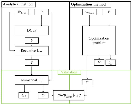
Figure 2.
Flowchart of the procedure. With slight abuse of notation and for the sake of readability, the subscripts are omitted. Note: V—voltage magnitudes at all network buses; ϕ—the active power flows, as calculated; ϕTerna—the active power flows, as provided by Terna; δLF—phase angles provided by exact calculations; δ—phase angles, as estimated by the DCLF procedure; ε—a threshold value for evaluation of accuracy of the results in terms of deviation from Terna’s dataset.
In the flowchart, δ denotes the voltage phases evaluated according to Equation (5), and δLF denotes the voltage phases resulting from the numerical LF.
The main goal of the two methods is the evaluation of voltage amplitudes at each node, which represent the lacking LF assignment, starting from the active power injections P and active power flows ΦTerna provided by Terna.
The optimization problem is able to evaluate—thanks to its mathematical formulation—the values of δLF and also the values of actual active power flows Φ. On the other hand, the analytical method requires a further numerical LF in order to calculate the values of δLF and Φ.
Finally, a validation procedure is performed in order to verify that, in absolute terms, the difference between the actual active power flows Φ and the values provided by Terna ΦTerna is less than an acceptable threshold ε for each line.
As a final comment, it should be noted that the origin of this study is an input of Terna; Terna needs to know the primary regulating energy and inertia gaps, which will appear in the Italian Transmission Network in the 2030 scenario, and how to cover them. For this reason, the final aim of this study is to decide (i) how to cover this possible gap, sharing it among the different technologies, which could participate in frequency support services, and (ii) where to place such resources. Of course, this cannot be performed punctually in every node of the Italian transmission network (sometimes, there are constraints other than the ones suggested by LF analysis). For this reason, the Italian TSO itself divided the Italian peninsula into seven market zones, relevant to the Italian energy market. The subdivision is provided in Attachment A.24 of the Italian grid code. Therefore, it was necessary to define a methodology for obtaining LF assignments consistent with the available data, which would work on this specific network structure. In addition, the optimization method could be replicated in any transmission network with a general topology, while the analytical method exploits the radial structure of the Italian simplified network, and therefore, it could only be applied in networks with the aforementioned topology.
3. Results
As specified in the Introduction, the active power injections and flows are available for all 8760 h of 2030. For the sake of brevity, a set of three hours was chosen in order to present the results of the two developed methods; these hours are considered critical for the Italian transmission network. The first hour (07:00 AM, 22 March 2030) is characterized by the largest active power exchanges with the foreign countries, for which a loss of the connection lines would trigger a severe transient. The second hour (02:00 PM, 9 April 2030) is characterized by a large RES penetration, meaning that low levels of inertia and primary regulating energy would be available in case of a frequency transient. The third hour (09:00 PM, 25 August 2030) is characterized by a large value of the rate of change of frequency following the ENTSO-E standard-defined contingency of loss of 3 GW of generation (standard value codified by ENTSO-E [6]).
The input data for the scenario are sensitive data for Terna; for this reason, the active power injections provided and the active power flows provided cannot be disclosed. In any event, in order to enhance the reader’s understanding, the main input quantities of the two methods are recalled in Table 1.

Table 1.
Main input quantities of the two methods.
Moreover, such validation is performed for all the remaining hours, with similar performances among the two proposed approaches (details are omitted for confidentiality reasons).
It should be noted that there are no theoretical reasons to obtain the same results with the application of the two methods. Given a network characterized by assigned values of the bus active power injections and branch active power flows, there are no theorems, which ensure that only one set of voltage amplitudes consistent with those input data exists.
Consequently, in what follows, the results of the two methods are presented together for each hour only for the purpose of readability. The two aspects, which have to be thoroughly checked, are (i) the phasors of voltages (to ensure that amplitudes belong to the admissibility range and that angles are not too far from zero in order to avoid an equilibrium point, which is likely to give origin to an unstable simulation from the transient stability standpoint) and (ii) deviations in the obtained active power flows in the branches compared to the input data.
It should be noted that, on the one hand, the optimization method is self-consistent because LF equations are inserted in the method’s constraints; on the other hand, the analytical method needs a classical LF calculation as post-processing to evaluate the exact values of phase angles, the active power flows and all the other quantities of interest (in what follows, the term “analytical method” will refer to a combination of the method described in the previous section and the post-processing LF calculation).
Before presenting the results, it has to be highlighted that the numerical values of the limits appearing in Equation (4) are Vmin = 0.95 p.u., Vmax = 1.05 p.u., δmin = −35°, δmax = 35°. The voltage limit values were set in accordance with the Italian grid code. In Equation (2), the ratio between the two weight coefficients, α/β, was considered equal to 1000. The ratio was chosen, such that the two terms of the objective function have the same order of magnitude.
The two methods are implemented in Matlab environment. The calculator used for the calculations is equipped with a 12th Gen Intel(R) Core(TM) i7-12700H 2.30 GHz CPU and a 16 GB RAM.
In more detail, in order to find the lacking LF assignments, the optimization problem associated with the optimization method is solved thanks to the Matlab function “fmincon”, while the analytical method itself does not require a numerical solver. The solver chosen among the ones embedded in fmincon is the default one, belonging to the family of interior-point methods; the approach of these methods to constrained minimization consists of the solution of an approximate minimization problem, comprising a sequence of equality-constrained problems, which are easier to solve than the original problem with inequality constraints [31].
It is important to highlight that fmincon is a local solver, and therefore, it is not applied to finding a global optimum. Moreover, the constraints of the optimization problem are strongly non-linear, and, as a consequence, the existence of a global minimum is not guaranteed from a theoretical point of view; in fact, it cannot be demonstrated that the optimization problem is a convex problem. In any event, the main aim of the methods is to find a set of canonical LF assignments resulting in active power flows, which are as close as possible to the ones provided by the TSO; in principle, any set of canonical LF assignments, which allows us to find a solution characterized by active power flows, which are quite close to the input data, is acceptable for the study purpose.
For the validation step, which consists of solution of the LF problem, the Matlab function “fsolve” is employed in order to solve the non-linear set of equations characterizing the LF problem itself. The solver chosen is the default one, i.e., the trust-region dogleg algorithm [32].
Table 2 shows the comparison between the computation times required for the solution of the two methods for each hour considered.
Table 2.
Computation times for the three hours considered.
In order to highlight the reliability of the methods, for each hour considered, the voltage amplitude and voltage phase at each node of the network are shown first in order to verify that they are within feasible ranges both for the optimization and the analytical method. Second, in order to complete the validation of the results, the deviation in the active power flows calculated from the ones provided by Terna within the input dataset is shown for both methods. The results are shown dimensionless due to a non-disclosure agreement concluded between Terna and the authors for confidentiality reasons.
Table 3 shows the voltage amplitude and phases obtained through the two methods for the hour characterized by large active power flows with foreign countries (07:00 AM, 22 March 2030). The voltage amplitudes are within the desired range, and the phase angles are all limited in quite narrow neighborhood of 0, which indicates the soundness of both proposed methods.
Table 3.
Voltage amplitudes—7 AM, 22 March 2030.
Table 4 shows the percentage deviations in the active power flows calculated from the input data and the active power losses in each branch, expressed in percentages based on the active power flows calculated. It is evident that, for both methods, the deviation in active power flows is smaller than 4%, and active power losses are smaller than 2%.
Table 4.
Active power flow deviation from the data provided by Terna—7 AM, 22 March 2030.
Table 5 shows the voltage amplitude and phases obtained through the two methods for the hour characterized by high penetration of RES (2 PM, 9 April 2030).
Table 5.
Voltage amplitudes—2 PM, 9 April 2030.
The voltage amplitudes are within the desired range, even if this range is broader than before; the phase angles are all limited to a much wider neighborhood of 0. However, in spite of not having implemented any constraints on these angles, the results of the analytical method in terms of phase angles slightly exceed 30 degrees.
Table 6 shows the percentage deviations in the active power flows calculated from the input data and the active power losses in each branch, expressed in percentages based on the active power flows calculated.
Table 6.
Active power flow deviation from the data provided by Terna—2 PM, 9 April 2030.
As one can see, for both methods, both deviations in active power flows from the values provided by Terna and active power losses are limited within the 3% margin.
Table 7 shows the voltage amplitude and phases obtained through the two methods for the hour characterized by a high value of RoCoF (9 PM, 25 August 2030).
Table 7.
Voltage amplitudes—9 PM, 25 August 2030.
As in the second hour considered, the voltage amplitudes are within the desired range; the phase angles, as dictated by the optimization method, never exceed 25 degrees. On the other hand, the maximum phase shift predicted by the analytical method occurs at bus 6, assuming a value of 31.3 degrees (the absence of constraints on the phase shift may explain these larger values).
Table 8 shows the percentage deviations in the active power flows calculated from the input data and the active power losses in each branch, expressed in percentages based on the active power flows calculated.
Table 8.
Active power flow deviation from the data provided by Terna—9 PM, 25 August 2030.
Again, both methods provide reliable results in terms of deviation in the active power flows from the values provided by Terna, limiting it to a few percentage points. The analytical method presents lower active power losses compared to the results of the optimization method.
In order to strengthen the reliability of the results, some error metrics may be considered for the evaluation of deviation in the active power flows calculated from the values provided by Terna—for example, the mean absolute error (MAE), root mean square error (RMSE) and the coefficient of variation of RMSE (cvRMSE), as defined, respectively, in Equations (9)–(11).
The values of the aforementioned indicators are reported in Table 9 for each hour considered.
Table 9.
Error metric indicators associated with active power flows for the three hours considered and for both methods.
The MAE and RMSE values are acceptable for both methods, considering that the values of power flows between the market zones are in the order of magnitude of hundreds of MW, or even in the order of magnitude of some GW. The most representative error metric is cvRMSE, which is the normalized measure of the error; its values, expressed in percentage, are very close to 0, meaning that the two methods are calibrated well.
Since tests were carried out for the whole year of 2030, the hourly trend of cvRMSE is represented in the two graphs in Figure 3 for both methods. It is evident in the figure that both methods return results, which are characterized by cvRMSE values, which are quite close to 0% for the whole year. This means that the accuracy of the methods in finding the missing LF assignments is satisfactory, leading to LF results—in terms of active power flows—which are close to the values provided by Terna.
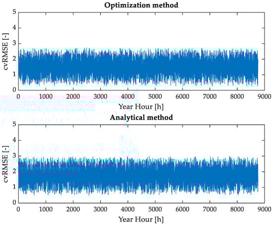
Figure 3.
Hourly trend of cvRMSE associated with active power flows for both methods.
Starting with the numerical results shown above, the advantages and disadvantages of the two developed methods—both showing effectiveness in providing a set of LF assignments consistent with the available input data (which is the main aim of the whole procedure)—can be discussed.
First, it should be clarified that the two methods represent independent alternatives for obtaining the missing LF assignments.
The advantage of the optimization method is that it provides a solution set in which voltage amplitudes and phases are limited within physically acceptable values by construction. Moreover, the insertion of deviation in the active power flows in the objective function is likely to ensure that a set of assignments compliant with the input data is obtained. In case of unsatisfactory results from this last point of view, the values of weight coefficients α and β can be changed in order to give more emphasis to the necessity for limiting active power flow deviation. Finally, this approach could be applied to any network with any topology.
On the other hand, the analytical method presents the advantage of having a simpler formalization; being totally analytical, its implementation is actually very easy, since it is simply a matter of inverting a matrix and calculating the first N-1 terms of a recursive law.
Moreover, there is no need for having an optimization method toolbox, and the computational effort is basically negligible.
Nevertheless, since this method does not involve the presence of constraints within its mathematical formulation, it does not offer the possibility of controlling the values of voltage amplitude at each node, which may assume unacceptable values. If this occurs, one could think of changing the value of Vslack in order to find a better solution. Finally, it should be noted that the analytical method fully exploits the in–out structure of the network; in fact, Equation (8) does not apply to a generic topology.
4. Conclusions
For the characterization of the future Italian scenario, the Terna development plan provides a dataset related to the forecasting of generation, load and active power flows in AC and HVDC lines for each hour and for each market zone for the whole year of 2030.
In order to set up a proper LF calculation—which is necessary to define the hourly working point of the Italian network—the input data had to be managed in order to find the usual LF assignments (i.e., voltage amplitude and active power injection at each equivalent node of the Italian network). This paper proposed two methods for the aforementioned purpose: the first one in the form of an optimization method, which is able to minimize the deviation in voltages at each bus from the rated value while also minimizing the deviation in active power flows from the input values; the second one in the form of a linear analytical method, which first estimates the voltage phase at each node by means of a DCLF and then evaluates the voltage amplitudes by means of a recursive law.
A set of three hours was chosen to test the two methods. The first hour was characterized by large active power flows with foreign bordering countries; the second hour was characterized by large RES penetration; and the third hour presented a high value of RoCoF. For all three hours, both methods showed acceptable results, keeping the voltage amplitude at each bus close to the rated value and the active power flow deviations within a few percentage points. Voltage phases assumed acceptable values, even if slightly exceeding 30 degrees at some buses. The advantages and disadvantages of both methods were thoroughly discussed; the main point is that the optimization method forces the quantities into a desired range and is suitable for any network, regardless of its topology. On the other hand, the analytical method does not require any optimization method toolbox, and its computational burden is almost negligible. The computation time for both methods is limited to less than half a second, with the analytical method being faster (between three and five times faster) due to the fact that it does not rely on a numerical solver, which is required for the solution of the optimization method. The accuracy of the results, compared with the dataset provided by Terna, is acceptable; the cvRMSE is very close to 0 for the whole year, being—on average—equal to 1.46% for the optimization method and 1.56% for the analytical method. Therefore, both methods are reliable, and the choice of one method over the other depends on the previously listed respective advantages and disadvantages.
Future developments may involve the application of the proposed methodology to more complex networks with different topologies.
Author Contributions
Conceptualization, R.P. and M.F.; methodology, R.P. and M.F.; software, M.F. and M.M.; validation, M.F. and M.M.; formal analysis, A.B.; resources, G.L. and L.O.; data curation, G.L. and L.O.; writing—original draft preparation, M.F. and M.M.; writing—review and editing, A.B. and R.P.; project administration, G.L. and L.O. All authors have read and agreed to the published version of the manuscript.
Funding
This research was funded by Terna S.p.A.
Data Availability Statement
3rd Party Data–Restrictions apply to the availability of these data, due to confidentiality reasons.
Conflicts of Interest
Authors Giuseppe Lisciandrello and Luca Orrù were employed by the company Terna S.p.A. The remaining authors declare that the research was conducted in the absence of any commercial or financial relationships that could be construed as a potential conflict of interest. The authors declare that this study received funding from Terna S.p.A. The funder had the following involvement within the study: collection and interpretation of data.
References
- Impram, S.; Nese, S.V.; Oral, B. Challenges of renewable energy penetration on power system flexibility: A survey. Energy Strategy Rev. 2020, 31, 100539. [Google Scholar] [CrossRef]
- Fresia, M.; Bracco, S. Electric Vehicle Fleet Management for a Prosumer Building with Renewable Generation. Energies 2023, 16, 7213. [Google Scholar] [CrossRef]
- AhmadiAhangar, R.; Plaum, F.; Haring, T.; Drovtar, I.; Korotko, T.; Rosin, A. Impacts of grid-scale battery systems on power system operation, case of Baltic region. IET Smart Grid 2024. [Google Scholar] [CrossRef]
- Sinsel, S.R.; Riemke, R.L.; Hoffmann, V.H. Challenges and solution technologies for the integration of variable renewable energy sources—A review. Renew. Energy 2020, 145, 2271–2285. [Google Scholar] [CrossRef]
- Tielens, P.; Van Hertem, D. The relevance of inertia in power systems. Renew. Sustain. Energy Rev. 2016, 55, 999–1009. [Google Scholar] [CrossRef]
- ENTSO-E. Need for Synthetic Inertia (SI) for Frequency Regulation; ENTSO-E: Brussels, Belgium, 2017. [Google Scholar]
- Minetti, M.; Fresia, M. A Review of Primary and Secondary Control for Islanded No-Inertia Microgrids. In Proceedings of the 2021 IEEE International Conference on Environment and Electrical Engineering and 2021 IEEE Industrial and Commercial Power Systems Europe (EEEIC/I&CPS Europe), Bari, Italy, 7–10 September 2021; pp. 1–7. [Google Scholar]
- Chawda, G.S.; Shaik, A.G.; Shaik, M.; Padmanaban, S.; Holm-Nielsen, J.B.; Mahela, O.P.; Kaliannan, P. Comprehensive review on detection and classification of power quality disturbances in utility grid with renewable energy penetration. IEEE Access 2020, 8, 146807–146830. [Google Scholar] [CrossRef]
- Bajaj, M.; Singh, A.K. Grid integrated renewable DG systems: A review of power quality challenges and state-of-the-art mitigation techniques. Int. J. Energy Res. 2020, 44, 26–69. [Google Scholar] [CrossRef]
- Anees, A.S. Grid integration of renewable energy sources: Challenges, issues and possible solutions. In Proceedings of the 2012 IEEE 5th India International Conference on Power Electronics (IICPE), Delhi, India, 6–8 December 2012; pp. 1–6. [Google Scholar]
- Nguyen, H.T.; Yang, G.; Nielsen, A.H.; Jensen, P.H. Combination of synchronous condenser and synthetic inertia for frequency stability enhancement in low-inertia systems. IEEE Trans. Sustain. Energy 2018, 10, 997–1005. [Google Scholar] [CrossRef]
- Lone, A.H.; Gedam, A.I.; Sekhar, K.R. Voltage Support and Imbalance Mitigation during Voltage Sags by Renewable Energy Fed Grid Connected Inverters. In Proceedings of the 2023 IEEE IAS Global Conference on Renewable Energy and Hydrogen Technologies (GlobConHT), Male, Maldives, 11–12 March 2023; pp. 1–6. [Google Scholar]
- Nguyen, H.T.; Yang, G.; Nielsen, A.H.; Jensen, P.H. Challenges and research opportunities of frequency control in low inertia systems. In E3S Web of Conferences, Proceedings of the 2019 The 2nd International Conference on Electrical Engineering and Green Energy (CEEGE 2019), Rome, Italy, 28–30 June 2019; EDP Sciences: Les Ulis, France, 2019; p. 02001. [Google Scholar]
- Pestana, R.; Khan, S.H.; Agreira, C.F. Optimum Voltage Droop Control in Transmission Systems to Support the Local Voltage Stability with High Share of RES. In Proceedings of the 2021 13th IEEE PES Asia Pacific Power & Energy Engineering Conference (APPEEC), Kerala, India, 21–23 November 2021; pp. 1–7. [Google Scholar]
- Shang, L.; Dong, X.; Liu, C.; Gong, Z. Fast grid frequency and voltage control of battery energy storage system based on the amplitude-phase-locked-loop. IEEE Trans. Smart Grid 2021, 13, 941–953. [Google Scholar] [CrossRef]
- Lal, N.K.; Mubeen, S.E. A review on load flow analysis. Int. J. Innov. Res. Dev. 2014, 3, 337–341. [Google Scholar]
- Andersson, G. Modelling and Analysis of Electric Power Systems; ETH Zurich: Zurich, Switzerland, 2008; pp. 5–6. [Google Scholar]
- Grisales-Noreña, L.F.; Morales-Duran, J.C.; Velez-Garcia, S.; Montoya, O.D.; Gil-González, W. Power flow methods used in AC distribution networks: An analysis of convergence and processing times in radial and meshed grid configurations. Results Eng. 2023, 17, 100915. [Google Scholar] [CrossRef]
- Bonfiglio, A.; Delfino, F.; Invernizzi, M.; Labella, A.; Mestriner, D.; Procopio, R.; Serra, P. Approximate characterization of large Photovoltaic power plants at the Point of Interconnection. In Proceedings of the Universities Power Engineering Conference, Stoke-on-Trent, UK, 1–4 September 2015. [Google Scholar]
- Grainger, J. Power System Analysis; McGraw-Hill: New York, NY, USA, 1999. [Google Scholar]
- Borkowska, B. Probabilistic load flow. IEEE Trans. Power Appar. Syst. 1974, 3, 752–759. [Google Scholar] [CrossRef]
- Chen, P.; Chen, Z.; Bak-Jensen, B. Probabilistic load flow: A review. In Proceedings of the 2008 3rd International Conference on Electric Utility Deregulation and Restructuring and Power Technologies, Nanjing, China, 6–9 April 2008; pp. 1586–1591. [Google Scholar]
- Allan, R.; Da Silva, A.L.; Burchett, R. Evaluation methods and accuracy in probabilistic load flow solutions. IEEE Trans. Power Appar. Syst. 1981, 5, 2539–2546. [Google Scholar] [CrossRef]
- Huang, Y.-F.; Werner, S.; Huang, J.; Kashyap, N.; Gupta, V. State estimation in electric power grids: Meeting new challenges presented by the requirements of the future grid. IEEE Signal Process. Mag. 2012, 29, 33–43. [Google Scholar] [CrossRef]
- Winter, A.; Igel, M.; Schegner, P. Supervised Learning Approach for State Estimation in Distribution Systems with missing Input Data. In Proceedings of the 2021 IEEE PES Innovative Smart Grid Technologies Europe (ISGT Europe), Espoo, Finland, 18–21 October 2021; pp. 1–5. [Google Scholar]
- Bonfiglio, A.; Fresia, M.; Minetti, M.; Procopio, R.; Rosini, A.; Lisciandrello, G.; Orrù, L. Inertia Requirements Assessment for the Italian Transmission Network in the Future Network Scenario. In Proceedings of the 2023 IEEE Belgrade PowerTech, Belgrade, Serbia, 25–29 June 2023; pp. 1–5. [Google Scholar]
- Fresia, M.; Minetti, M.; Rosini, A.; Procopio, R.; Bonfiglio, A.; Invernizzi, M.; Denegri, G.B.; Lisciandrello, G.; Orrù, L. A Techno-Economic Assessment to Define Inertia Needs of the Italian Transmission Network in the 2030 Energy Scenario; IEEE Transactions on Power Systems: Piscataway, NJ, USA, 2023; pp. 1–12. [Google Scholar]
- TERNA. Documento di Descrizione degli Scenari; TERNA: Rome, Italy, 2022. [Google Scholar]
- TERNA. Allegato A.24 al Codice di Rete; TERNA: Rome, Italy, 2021. [Google Scholar]
- Marconato, R. Steady State Behavior Controls, Short Circuits and Protection Systems; Electric Power Systems: North Logan, UT, USA, 2004; Volume 2. [Google Scholar]
- Nocedal, J.; Öztoprak, F.; Waltz, R. An interior point method for nonlinear programming with infeasibility detection capabilities. Optim. Methods Softw. 2014, 29, 837–854. [Google Scholar] [CrossRef]
- MathWorks Italia. Solve System of Nonlinear Qquations-MATLAB fsolve. Available online: https://it.mathworks.com/help/optim/ug/fsolve.html#bqbnh0l-1 (accessed on 20 January 2024).
Disclaimer/Publisher’s Note: The statements, opinions and data contained in all publications are solely those of the individual author(s) and contributor(s) and not of MDPI and/or the editor(s). MDPI and/or the editor(s) disclaim responsibility for any injury to people or property resulting from any ideas, methods, instructions or products referred to in the content. |
© 2024 by the authors. Licensee MDPI, Basel, Switzerland. This article is an open access article distributed under the terms and conditions of the Creative Commons Attribution (CC BY) license (https://creativecommons.org/licenses/by/4.0/).