Prediction of ORF for Optimized CO₂ Flooding in Fractured Tight Oil Reservoirs via Machine Learning

Abstract

Tight reservoirs characterized by complex physical properties pose significant challenges for extraction. CO₂ flooding, as an EOR technique, offers both economic and environmental advantages. Accurate prediction of recovery rate plays a crucial role in the development of tight oil and gas reservoirs. But the recovery rate is influenced by a complex array of factors. Traditional methods are time-consuming and costly and cannot predict the recovery rate quickly and accurately, necessitating advanced multi-factor analysis-based prediction models. This study uses machine learning models to rapidly predict the recovery of CO₂ flooding for tight oil reservoir development, establishes a numerical model for CO₂ flooding for low-permeability tight reservoir development based on actual blocks, studies the effects of reservoir parameters, horizontal well parameters, and injection-production parameters on CO₂ flooding recovery rate, and constructs a prediction model based on machine learning for the recovery. Using simulated datasets, three models, random forest (RF), extreme gradient boosting (XGBoost), and light gradient boosting machine (LightGBM), were trained and tested for accuracy evaluation. Different levels of noise were added to the dataset and denoised, and the effects of data noise and denoising techniques on oil recovery factor prediction were studied. The results showed that the LightGBM model was superior to other models, with R² values of 0.995, 0.961, 0.921, and 0.877 for predicting EOR for the original dataset, 5% noise dataset, 10% noise dataset, and 15% noise dataset, respectively. Finally, based on the optimized model, the key control factors for CO₂ flooding for tight oil reservoirs to enhance oil recovery were analyzed. The novelty of this study is the development of a machine-learning-based method that can provide accurate and cost-effective ORF predictions for CO₂ flooding for tight oil reservoir development, optimize the development process in a timely manner, significantly reduce the required costs, and make it a more feasible carbon utilization and EOR strategy.

1. Introduction

There has been a growing emphasis on exploring and developing unconventional oil and gas resources worldwide. But extracting residual oil from tight reservoirs in complex geological formations remains a significant challenge [1]. Numerous studies have demonstrated the significant impact of CO₂ flooding on enhancing oil recovery (EOR) in low-permeability reservoirs [2,3,4,5]. CO₂ flooding holds the potential for achieving high efficiency in extracting oil from reservoirs. However, the development of CO₂ flooding in tight reservoirs is affected by various factors, such as geology, fluid properties, CO₂ phase transition, and fracture structure modification, which pose challenges for predicting oil recovery factors for CO₂ flooding [6].

Additionally, different oil recovery factors can characterize the different development stages of the current oil and gas field [7]. Through the prediction of recovery, real-time production control can be achieved, production measures can be adjusted in a timely manner, and reservoir development can be optimized. Therefore, accurate prediction of recovery rate plays a crucial role in the development of oil and gas fields.

Currently, oil recovery factor prediction in tight oil reservoirs mainly revolves around water-driven development. The prediction methods can be broadly categorized into three main approaches: macro-equilibrium analysis, micro-experimental mechanistic analysis, and numerical simulation method [8,9,10,11,12,13,14,15]. Sun et al. [16] developed a power-function-based material balance equation for high-pressure and ultrahigh-pressure gas reservoirs and investigated the impact of reservoir pressure depletion and recovery degree on reserve estimation reliability. Cheng et al. [17] proposed a synchronization iterative oilfield oil recovery factor prediction method by combining water content curves with the exponential decline method, which is based on statistical regression experiments and field data through Buckley–Leverett theory, and these approaches have improved accuracy of oilfield recovery factor prediction. Hadia et al. [18] conducted core drive experiments to analyze the relationship between relative permeability and water saturation and predicted the recovery degree through a numerical simulation model based on the dimensionless Buckley–Leverett equation. Zhong et al. [19] studied the recovery efficiency of CO₂ flooding timing and different injection methods based on the reservoir conditions of a block in Jilin Oilfield using Eclipse 3.0. Nevertheless, the main factors affecting the recovery of CO₂ flooding in tight oil reservoirs are complex and diverse. The Macroscopic Balance Analysis and Microscopic Experimental Mechanics Analysis methods can only provide rough estimates of recovery rates, lacking precision and incurring high costs. Numerical simulation techniques require individual modeling for different reservoirs, with prediction accuracy dependent on field data, and involve lengthy simulation times. Their accuracy hinges on the availability of accurate field data, and these simulations typically require extended periods to complete. Therefore, further research is needed on the recovery prediction model for CO₂ flooding in fractured tight oil reservoirs.

In contrast, machine learning (ML) methods offer a distinct advantage. They can create unique predictive models that consider various reservoir characteristics, uncover hidden data relationships, and accurately predict production outcomes at a lower cost. In the petroleum industry, ML models have been widely applied and achieved good application results. In the petroleum industry and underground gas storage, machine learning has found application in a myriad of areas, including the evaluation of reserves in both conventional and unconventional reservoirs [20,21,22,23], the automated interpretation of well tests [24,25,26,27], forecasting production from oil and shale gas [28,29,30,31], as well as in predicting the lithology of reservoirs [32,33,34]. ML models have also been utilized in research for enhanced oil recovery (EOR). Van Si et al. [35] developed an artificial neural network (ANN) model designed to forecast the oil recovery factor (ORF) specific to CO₂-enhanced oil recovery (EOR) processes. Cheraghi et al. [36] suggested employing deep ANN and random forest (RF) models for identifying the most appropriate EOR techniques, leveraging data sourced from oil and gas publications. Esene et al. [37] conducted predictions of the ORF using ANN, least-squares support vector machines, and gene expression programing for carbonate water-injection processes. In another study, Pan et al. [38] constructed a machine learning model utilizing extreme gradient boosting (XGBoost) to infer reservoir porosity from well log data. They enhanced the XGBoost model’s accuracy through a combination of grid search and nature-inspired optimization methods, achieving a root mean square error (RMSE) of 0.527. Further extending the exploration of machine learning applications, Huang et al. [39] evaluated the performance of ANNs, light gradient boosting machine (LightGBM), and XGBoost models in forecasting production from steam-assisted gravity drainage processes. Collectively, these investigations underscore the significant capabilities of machine learning models in forecasting the oil recovery factor and enhancing oil recovery methodologies. Compared to traditional methods of predicting recovery rates, ML can deeply mine the relationship between complex data and recovery, extract data features to identify the main controlling factors affecting recovery rates, and efficiently, accurately, and cost-effectively predict the recovery rates of reservoirs under different geological conditions. While previous research has explored machine learning (ML) models, their application in the rapid prediction of CO₂ flooding systems in tight oil reservoirs has not been extensively studied. Given the difficulty of accurately simulating underground fracturing conditions in laboratory settings and the associated high costs, the majority of recent studies have turned to numerical simulations to gather data. However, these studies frequently neglect the effect of data noise on their outcomes, potentially leading to variances between the research conclusions and real-world scenarios.

Therefore, the study is dedicated to crafting and evaluating a range of ML models to find the optimal one for application. The goal is to identify a model that significantly reduces both the time and financial costs associated with experiments while ensuring the precision of predictions regarding the ORF in the context of CO₂ flooding through horizontal wells in tight oil reservoirs, thereby providing valuable insights for future gas injection strategies in these reservoirs. For testing these models, we considered a wide array of production and geological parameters, compiling a comprehensive dataset. To more accurately reflect real-world conditions, we introduced noise into the dataset and then applied denoising techniques. This approach allows us to assess the impact of noise and denoising on our research outcomes. The findings of our study present an effective solution for swiftly predicting the ORF of CO₂ flooding in tight oil reservoirs and have potential applications in other EOR methods.

2. Methodology

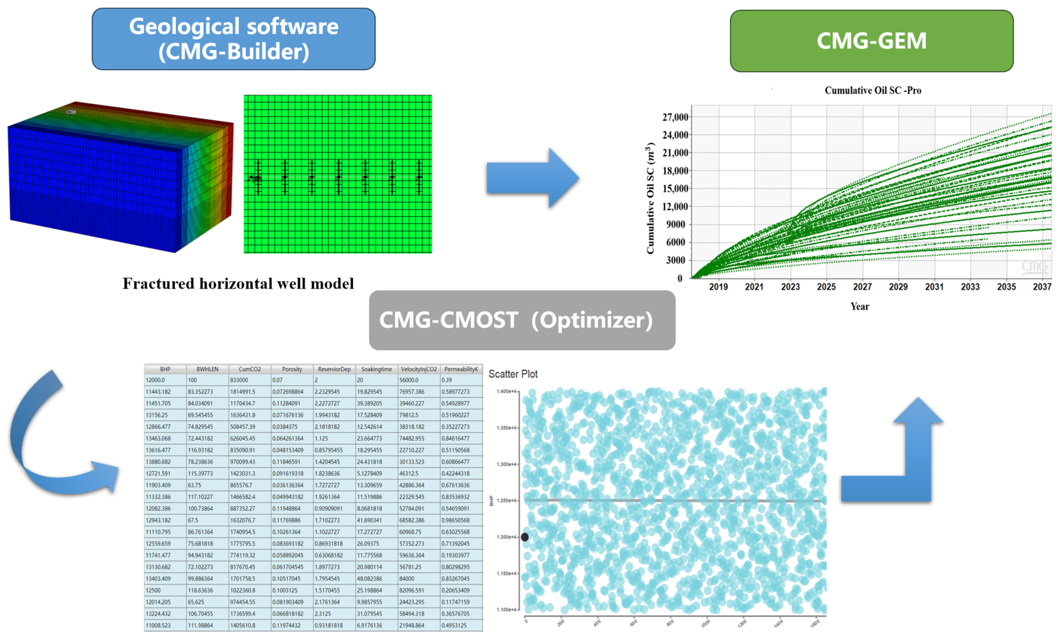
This section outlines the core workflow of a novel prediction method for CO₂ Enhanced Oil Recovery (CO₂-EOR) rates. Initially, a numerical model is developed, drawing on real-world development scenarios. Key factors that influence CO₂-EOR rates are determined from prior studies. Then, using Latin hypercube sampling (LHS), a dataset for numerical simulation is created. To enhance the dataset’s realism and quality, it is further processed through noise addition and denoising techniques. A general workflow for ML-based prediction of recovery degree is illustrated in Figure 1. The specific steps of the work are described in detail in the following subsections.

2.1. Data Preparation

2.1.1. Reservoir Model Description

Changqing tight reservoir, ideal for CO₂ miscible flooding due to its vast area and access to substantial gas resources, is the chosen site for CO₂ injection. The project is further supported by favorable on-site road conditions. To model the CO₂ injection process accurately without the influence of reservoir boundaries, we employed CMG-GEM numerical simulation software to create a simulation model. This model features a single-well radial grid layout measuring 2440 m × 1640 m × 26 m, covering 4 km². Utilizing the Cartesian grid system, the formation is divided into regular grids: 61 in the I direction, 41 in the J direction, and 13 in the K direction, with standard grid sizes of 40 m × 40 m × 2 m. The central encrypted grid is finer, with dimensions of 8 m × 8 m × 2 m. Figure 2 showcases the model’s 3D distribution and grid layout.

The original reservoir pressure is 20.9 MPa, the saturation pressure is 10.18 MPa, and the reservoir temperature is 84 °C. The porosity and permeability of the matrix are assumed to be uniformly distributed in this model. The boundary conditions, initial conditions, and specific parameters are presented in

Table 1. Reservoir parameter settings.

Parameters	Value	Units
Reservoir depth	2126	m
Reservoir pressure	20.9	MPa
Saturation pressure	10.18	MPa
Reservoir temperature	84	°C
Rock Compressibility	1 × 10−8	1/kPa
Permeability	0.39	mD
Porosity	0.071	-
Fracture conductivity	30	mD·m
Horizontal well length	1020	m
Fracture half-length	120	m
The maximum CO2 injection volume	1500	t
Injection rate of CO2	50	t/day
Minimum bottomhole flow pressure	11	MPa
Maximum surface oil rate	50	m3/d
Soaking time	20	d

.

The fluid phase data were fitted using the results of the formation fluid phase simulation and the fluid phase permeation curves were taken from phase permeation data derived from laboratory long-core testing experiments, as shown in Figure 3.

2.1.2. Obtaining Numerical Simulation Data

In the simulation process, continuous CO₂ injection into fractured horizontal wells was modeled over an 18-year period, with daily oil production rates varying between 1 m³/d and 2 m³/d. Following the screening criteria for CO₂ flooding as outlined by Carcoana et al. [21,40,41], this study aimed to refine ORF prediction accuracy and model applicability by considering a broader spectrum of factors and incorporating more detailed characteristic parameters.

To achieve this, the study gathered a large dataset through the definition of uncertainty variables and the application of Latin hypercube sampling, guided by previous sensitivity analyses that highlighted key factors in the EOR-CO₂ process [1,42,43,44,45]. Consequently, nine parameters were selected for detailed analysis: porosity (Por), permeability (Perm), reservoir thickness (Thickness), fracture half-length (FHL), bottom hole flowing pressure (BHP), injection rate of CO₂ (CO₂-INJ), cumulative injected CO₂ mass (CO₂-CMASS), soaking time (SOAK-T), and number of fractures (Numfrac). Based on the nine selected influential factors and using the parameter ranges provided in

Table 2. The range of values for the model parameters in the Latin hypercube experimental design.

Parameter	Symbol	Minimum	Maximum	Base Case	Units
Porosity	Por	0.03	0.12	0.071	-
Permeability	Per	0.05	1.05	0.39	mD
Reservior thickness	Thickness	6.5	35	26	m
Fracture half-length	FHL	60	120	100	m
Bottom hole flowing pressure	BHP	11	14	12	MPa
Injection rate of CO2	CO2-INJR	30	150	100	t/day
Accumulated injection mass of CO2	CO2-Mass	750	3500	1500	t
Soaking time	SOAK-T	5	50	20	day
Number of fractures	Numfrac	5	10	7	-

, Latin hypercube sampling (LHS) was applied to sample these nine parameters, resulting in 4090 data samples. And a new reservoir model was generated based on these 9 parameters. The CMOST optimization tool facilitated parallel computing to calculate the reservoir recovery rate 10 years later. It will take 16,360 min to obtain the calculation results of these 4090 models in this study. The integration of Builder and CMOST allows for the simulation of different geological implementations, as illustrated in Figure 4.

2.1.3. Data Preprocessing

In this study, the impact of noise addition and denoising on the dataset’s predictive results was investigated. Adding noise to the dataset aimed to improve the machine learning model’s generalization capacity, mitigating the risk of overfitting and accommodating wider data variability, thereby aligning the simulation more closely with real-world data. To further enhance the model’s performance and the precision of CO₂-EOR rate predictions, the study employed wavelet denoising techniques on the dataset with added noise, followed by a standardization process.

Obtaining Data with Noise

The dataset used in this section is derived from the reservoir numerical simulation model constructed in Section 2.1.2. It consists of a total of 4090 groups of data. Each group of models calculates the ORF for the corresponding model. The dataset includes the ORF and nine parameters mentioned in the previous section, namely Por, Per, Thickness, FHL, BHP, CO₂-MASS, CO₂-INJR, SOAK-T, and Numfrac, forming a set of data for each model.

In order to enhance the resemblance of the simulated data to the actual data collected in the field, we introduced different levels of noise to the simulated data. We added noise with the same noise ratio to all 4090 datasets, creating a noise dataset with the same noise level. Subsequently, we will assess the impact of noise corruption on the data.

The formula to add noise is represented by the following:

$$D_{noise}=D+\alpha \cdot D\cdot \epsilon$$

(1)

where $D$ is the original numerical simulation data, $\alpha$ is the noise level, and $\epsilon$ is the random number.

Three datasets were generated, each containing 4090 data points, with noise levels set at 0.05, 0.1, and 0.15, respectively. This study then examined how the predictive accuracy of machine learning models was impacted by these varying degrees of noise.

Obtaining Denoised Data

In practical applications, noise can interfere with the accurate analysis and processing of signals, leading to challenges in making precise judgments. In our previous section, we intentionally introduced random noise to analog data to simulate real-world conditions. Therefore, it becomes crucial to denoise the signal in order to enhance the quality of analysis and facilitate subsequent processing at various levels. To boost the model’s accuracy and refine our dataset, we employed an efficient and widely applicable wavelet denoising technique. This method was used to clean the datasets that had noise ratios of 0.05, 0.10, and 0.15, as identified in the earlier section of our study, The principle of wavelet denoising is as follows:

Assuming there is a noisy signal of length N:

$$D_{noise}(n)=D(n)+\alpha \cdot e(n)$$

(2)

where $D(n)$ is the truth data and $e(n)$ is the noise.

The WT involves concentrating the energy of a noisy signal in some of the larger wavelet coefficients after wavelet decomposition. In contrast, noise energy is spread throughout the wavelet domain, leading to smaller wavelet coefficients being predominantly influenced by noise. This property allows us to consider larger wavelet coefficients as the signal and smaller ones as the noise. Wavelets, with their decorrelation feature, play a crucial role in signal processing, image processing, data analysis, and prediction [46,47,48].

The continuous WT of a one-dimensional continuous function $D(n)$ is given by:

$$W_r(a,b):={\displaystyle {\int }_{-\infty }^{+\infty }D}(n)\overline{{\psi }_{a,b}(n)}dn=\frac{1}{\sqrt{\left|a\right|}}{\displaystyle {\int }_{-\infty }^{+\infty }D}(n)\overline{\psi \left(\frac{n-b}{a}\right)}dn$$

(3)

where $W_r(a,b)$ is the corresponding wavelet coefficient, ${\psi }_{a,b}(n)$ is the wavelet function, $\psi (n)$ is the fundamental wavelet, a is the scaling factor, and b is the translation factor.

On the other hand, the wavelet inversion is given by:

$$D(n):=C_{\psi }^{-1}{\displaystyle {\int }_{-\infty }^{+\infty }{\displaystyle {\int }_{-\infty }^{+\infty }{W}_r(a,b)}}{\psi }_{a,b}(n)\frac{da}{a^2}db$$

(4)

$$C_{\psi }={\displaystyle {\int }_{-\infty }^{+\infty }\frac{\left|\widehat{\psi (\omega )}\right|}{\left|\omega \right|}}d\omega <\infty$$

(5)

$\widehat{\psi (\omega )}$ is the Fourier transform of $\psi (n)$.

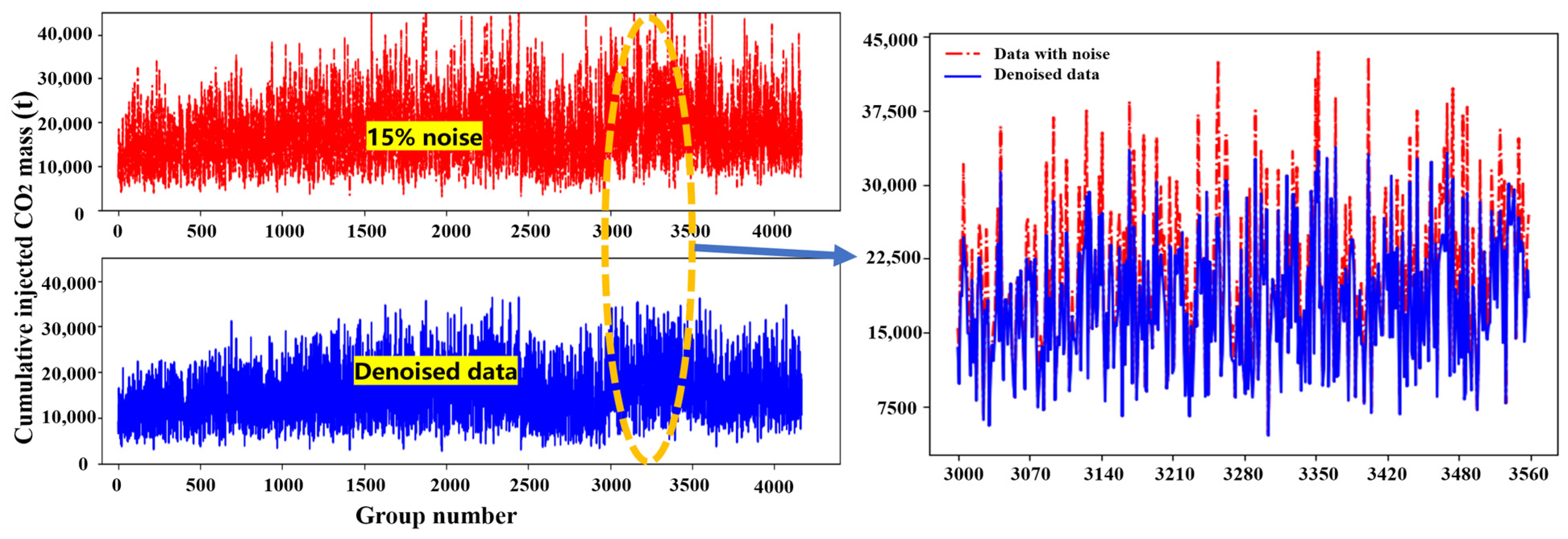
In the experiment, we utilized WT technology to filter the analog datasets with four different noise levels. Taking the example of cumulative injected CO₂ data with 15% noise, the comparison before and after filtering is depicted in Figure 5.

Data Normalization

To improve model generalization and accuracy, the original dataset from the simulation, the noisy dataset with added noise at different ratios, and the denoised dataset using WT are all normalized. This normalization removes the influence of scale and reduces data fluctuation interference, facilitating more reliable and meaningful comparisons and predictions. The normalization equation is as follows:

$$X=\frac{x-x_{\min }}{x_{\max }-x_{\min }}$$

(6)

where $X$ is the normalized data, $x_{\min }$ is the minimum value of this type of data, and $x_{\max }$ is the maximum value of this type of data.

2.2. Theory of Machine Learning Techniques

2.2.1. Random Forest

Random Forest (RF) serves as a multifunctional algorithm for both classification and regression, employing an ensemble approach to enhance prediction accuracy and stability. It constructs numerous regression trees from randomly selected subsets of the training data and predictors. Training each tree with bootstrap samples and applying binary splits on a chosen subset of predictors at every node, RF effectively selects features and grows trees. This methodology ensures the RF model’s effectiveness in diverse prediction scenarios by leveraging the collective strength of multiple trees for more reliable outcomes [49].

2.2.2. XGBoost

XGBoost is an advanced boosting ensemble method applied to both regression and classification, aimed at reducing training error by assembling weak learners into a robust combined model [50,51,52,53]. It begins with training an initial model on a randomly chosen data sample and employs incremental boosting to correct previous models’ errors. XGBoost’s distinctiveness lies in its objective function, which blends a loss function—to minimize the gap between predicted and actual values—with a regularization term to deter overfitting, ensuring a balance between accuracy and model simplicity.

2.2.3. Light Gradient Boosting Machine (LightGBM)

The LightGBM model, a recent advancement leveraging the gradient boosting tree technique, was selected for this study for its precision and scalability [54]. Its effectiveness is largely owed to its enhanced loss function, which builds upon the Taylor objective function with a second-order extension. This method captures more detailed information about the objective function, significantly improving model performance. The following is the mathematical form of the loss function:

$${\mathrm{L}}_{\mathrm{t}}={\displaystyle \sum _{\mathrm{j}=1}^{\mathrm{J}}\left[{\mathrm{G}}_{\mathrm{tj}}{\mathrm{w}}_{\mathrm{tj}}+\frac{1}{2}\left({\mathrm{H}}_{\mathrm{tj}}+\lambda \right){\mathrm{w}}_{\mathrm{tj}}^2\right]}+\gamma \mathrm{J}$$

(7)

$${\mathrm{G}}_{\mathrm{tj}}={\displaystyle \sum _{{\mathrm{x}}_{\mathrm{i}}\in {\mathrm{R}}_{\mathrm{tj}}}{\mathrm{g}}_{\mathrm{ti}}},{\mathrm{H}}_{\mathrm{tj}}={\displaystyle \sum _{{\mathrm{x}}_{\mathrm{i}}\in {\mathrm{R}}_{\mathrm{tj}}}{\mathrm{h}}_{\mathrm{ti}}}$$

(8)

where ${\mathrm{G}}_{\mathrm{tj}}$ and ${\mathrm{H}}_{\mathrm{tj}}$ represent the first and second derivatives of the objective function for each sample within a leaf-node area, respectively, ${\mathrm{w}}_{\mathrm{tj}}$ is the optimal value assigned to the Jth leaf node of each decision tree, J refers to the total count of leaf nodes, and $\gamma$ and $\lambda$ are user-defined values.

The information gain employed in the segmentation of each leaf node is:

$${\mathrm{Gain}}^{\prime }=\frac{1}{2}\left[\frac{{\mathrm{G}}_{\mathrm{J}}^2}{{\mathrm{H}}_{\mathrm{L}}+\lambda }+\frac{{\mathrm{G}}_{\mathrm{R}}^2}{{\mathrm{H}}_{\mathrm{R}}+\lambda }-\frac{{\left({\mathrm{G}}_{\mathrm{L}}+{\mathrm{G}}_{\mathrm{R}}\right)}^2}{{\mathrm{H}}_{\mathrm{L}}+{\mathrm{H}}_{\mathrm{R}}+\lambda }\right]-\gamma$$

(9)

Additionally, LightGBM shifts away from XGBoost’s level-wise approach to adopt a leaf-wise growth strategy with depth limitations, significantly boosting its efficiency. It selects the leaf with the highest splitting gain from all the existing leaves and performs splitting and cycling, achieving higher accuracy. However, it is important to note that this approach may occasionally result in overfitting. To mitigate this issue, the max_depth parameter can be set to control the depth of the tree and prevent excessive complexity.

Figure 6 illustrates the architecture of LightGBM. The LightGBM network model is built on the gradient-boosted decision tree (GBDT) algorithm framework and incorporates several techniques to enhance efficiency and accuracy. It utilizes Gradient-Based One-Side Sampling (GOSS) for sampling, reducing computational and time costs by focusing on relevant samples. The model also employs a histogram algorithm to find the best data segmentation points, reducing memory usage and segmentation complexity. Additionally, it uses a leaf node growth algorithm with a depth limit to improve accuracy and prevent overfitting. By leveraging these techniques, LightGBM achieves a balance between efficiency and accuracy, making it well suited for handling large datasets and delivering high-performance results.

Compared to XGBoost’s presorting algorithm, LightGBM optimizes time complexity from O (Data * features) to O (Bins * features). Additionally, the histogram-based algorithm consumes approximately seven times less memory than the presorting algorithm.

The EFB algorithm plays a role in reducing feature dimensions by converting numerous mutually exclusive features into low-dimensional dense features. This effectively avoids unnecessary calculations involving redundant features with zero values.

Overall, LightGBM offers the benefits of scalability and high accuracy. With the continuous expansion of oilfield datasets, LightGBM holds potential for applications in predicting the ORF for CO₂-EOR and even in practical field operations within the petroleum industry.

2.3. Workflow

The ML models were trained using the input variables: Por, Perm, Thickness, FHL, BHP, CO₂-CMASS, CO₂-INJR, SOAK-T, and Numfrac. Figure 1 illustrates the key processes involved in the proposed methodology.

2.3.1. Dataset Partitioning

In this study, as outlined in Section 2.1, we generated three datasets: original, noise-added, and denoised. We allocated 80% of each dataset for training the models, with the balance 20% reserved for performance evaluation. To ensure robust model validation, we employed 10-fold cross-validation, dividing the training segment into ten parts—nine for training and one for validation in turn. This technique allowed for the comprehensive utilization of data for training while preserving the integrity of the test set, thus yielding a more reliable measure of the model’s true accuracy.

2.3.2. ML Model Development

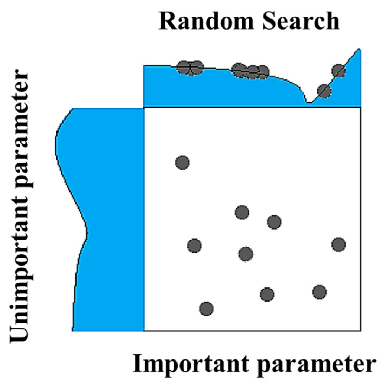
The random search method (Figure 7) is employed to identify hyperparameters using RMSE as the evaluation metric, aiming to enhance the model’s accuracy.

Table 3. Search range of selected hyperparameters.

Model	Hyperparameter	Range
RF	n_estimators	10, 50, 100, 300, 500
	max_depth	10, 20, 40, 70, 100
	min_samples_leaf	1, 2, 4, 6, 8
	max_features	0.2, 0.4, 0.7, 0.8, 1
	learning_rate	0.001, 0.01, 0.05, 0.1, 1
	min_samples_split	1, 2, 4, 6, 8
XGboost	n_estimators	10, 50, 80, 100, 200
	max_depth	1, 2, 4, 6, 8
	num_leaves	8, 16, 32, 64, 128
	learning_rate	0.001, 0.01, 0.05, 0.1, 1
	randam_state	0, 6, 12, 20, 30
	min_child_weight	0.1, 0.2, 0.4, 0.6, 0.8
	subsample	0.5, 0.6, 0.7, 0.8, 1
	colsample_bytree	0.5, 0.6, 0.7, 0.8, 1
LightGBM	n_estimators	50, 100, 300, 500, 800
	max_depth	3, 4, 5, 6, 7
	num_leaves	8, 16, 32, 64, 128
	learning_rate	0.01, 0.05, 0.1, 0.5, 1
	max_bin	10, 30, 50, 60, 70
	bagging_fraction	0, 0.1, 0.4, 0.7, 1
	bagging_freg	10, 40, 50, 60, 80
	bagging_seed	10, 20, 40, 60, 80
	Feature_fraction	0.5, 0.6, 0.7, 0.8, 0.9

shows the search range of selected hyperparameters of the three regression models based on RF, XGboost, and LightGBM at different noise levels.

2.3.3. Model Performance Evaluation

The evaluation indicators of the ORF prediction regression model were set as follows [55]: correlation factor (R²), root mean square error (RMSE), and mean absolute percentage error (MAE).

$${\mathrm{R}}^2=1-\frac{{\displaystyle {\sum }_{i=1}^N{(y_{pre}-y_{tru})}^2}}{{\displaystyle {\sum }_{i=1}^N{(\overline{y_{tru}}-y_{tru})}^2}}$$

(10)

$$\mathrm{RMSE}=\sqrt{\frac{1}{m}{\displaystyle \sum _{i=1}^m{\left(y_{tru}-y_{pre}\right)}^2}}$$

(11)

$$\mathrm{MAE}=\frac{1}{N}{\displaystyle \sum _{i=1}^N\left|y_{tru}-y_{pre}\right|}$$

(12)

3. Results and Discussion

This section focuses on assessing the proposed RF, XGBoost, and LightGBM models’ effectiveness in forecasting CO₂-EOR. We also examine how data noise and subsequent denoising actions affect the accuracy of model predictions. By analyzing data through these models, we have pinpointed critical factors that impact the CO₂ recovery in tight oil reservoirs, providing valuable insights for optimizing CO₂-EOR strategies in oilfields.

3.1. Evaluation of Model Performance

Hyperparameter tuning plays a crucial role in achieving optimal ML model performance. Consequently, for all types of ML models, the tuning process should be prioritized to guarantee the precision of the prediction model. As illustrated in

Table 4. Optimal parameters for different models.

Model	Hyperparameter	Optimal Value (Original Data)	Optimal Value (5% Noise)	Optimal Value (10% Noise)	Optimal Value (15% Noise)
RF	n_estimators	100	200	200	100
	max_depth	70	70	70	20
	min_samples_leaf	2	2	2	1
	max_features	0.7	0.7	0.8	0.8
	learning_rate	0.1	0.1	0.1	0.05
	min_samples_split	4	4	2	5
XGboost	n_estimators	80	80	100	100
	max_depth	4	4	6	6
	num_leaves	16	32	32	16
	learning_rate	0.1	0.1	0.1	0.05
	randam_state	9	12	20	20
	min_child_weight	0.6	0.8	0.8	0.8
	subsample	1	1	1	0.8
	colsample_bytree	1	1	1	0.8
Lightbgm	n_estimators	300	300	500	300
	max_depth	5	5	5	5
	num_leaves	32	32	32	32
	learning_rate	0.05	0.01	0.01	0.05
	max_bin	50	50	60	60
	bagging_fraction	0.6	0.7	0.6	0.4
	bagging_freg	40	40	50	80
	bagging_seed	40	40	60	60
	Feature_fraction	0.8	0.8	0.8	0.8

, we identified optimal parameters for RF, XGBoost, and LightGBM models across different noise levels by the random search method outlined in Section 2.3.2.

Table 5. Prediction accuracy of training and testing sets.

Data	Indicator	RF	XGboost	LightGBM
Training	R2	0.992	0.995	0.996
	RMSE	0.017	0.013	0.008
	MAE	0.011	0.010	0.009
Testing	R2	0.959	0.985	0.995
	RMSE	0.031	0.023	0.009
	MAE	0.018	0.014	0.010

illustrates the performance metrics (R², RMSE, and MAE) of each ML model based on the aforementioned hyperparameters and in predicting ORF using the original dataset. Generally, a higher R² and lower values of MAE and RMSE indicate better predictive accuracy. In the training phase, all models showed excellent results, with R² values exceeding 0.99. LightGBM was the standout, achieving an R² of 0.996, RMSE of 0.008, and MAE of 0.009. Its dominance extended to the testing phase, where it maintained high accuracy (R² = 0.995, RMSE = 0.009, and MAE = 0.010).

The data obtained from numerical simulations are typically free from noise interference but, in real-world measurements, data noise is unavoidable. Previous studies, Sun and Thanh et al. [7,52], have used numerical simulation data for machine learning models to evaluate CO₂ storage capacity and effectiveness. However, they did not consider the presence of noise in on-site data. To simulate the presence of noise in on-site data and enhance the generalization of the trained machine learning model in this study, we introduced different levels of noise using the method described in Section 2.1.3. Subsequently, we performed the denoising processing (Section 2.1.3) to investigate the impact of noisy data and denoised data on the prediction results of ORF.

3.2. Effect of Noise on the ML Model Oil Recovery Factor Predictions

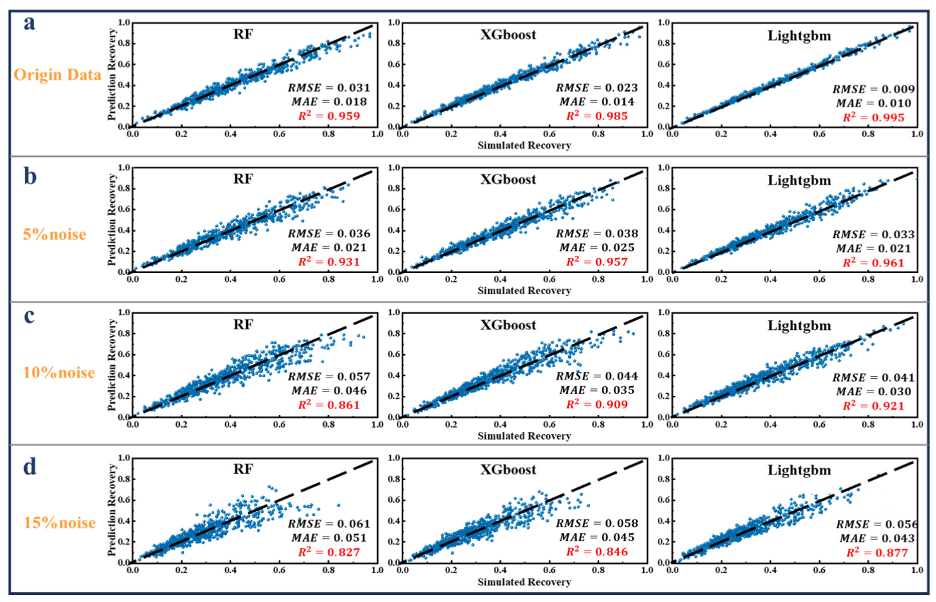
After adjusting the hyperparameters of the three machine learning models for ORF prediction (as presented in Table 4), we evaluated each model’s performance across diverse noise levels. Figure 8 shows that an increase in the noise ratio is associated with a discernible decline in the accuracy of the machine learning model’s predictions for recovery. Figure 8a demonstrates that, at a 5% noise level, the correlation coefficient between predicted and measured ORFs from test data predominantly aligns with the fitted line (slope = 1), indicating accurate predictions by RF, XGBoost, and LightGBM (R² > 0.95). In Figure 8b, the RF model’s R² significantly drops to 0.891 at a 10% noise level from 0.954 at 5% noise. However, XGBoost and LightGBM maintain strong accuracy (R² > 0.91). Figure 8c depicts that, at a 15% noise level, all models exhibit R² values below 0.87, RMSE values exceeding 0.055, and MAE values surpassing 0.043.

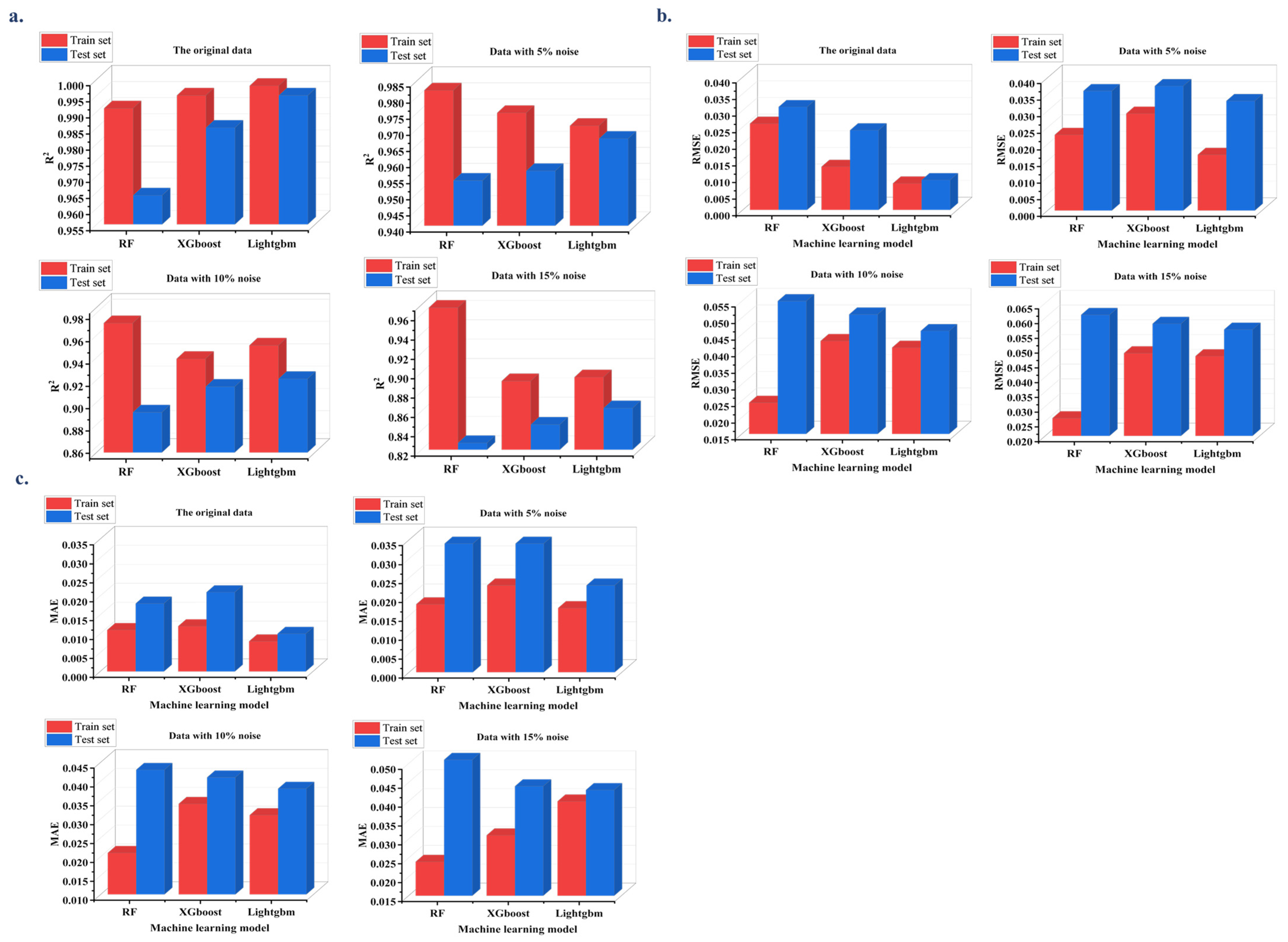
Figure 9 presents the relationship between predicted and simulated ORFs for CO₂ flooding in tight oil reservoir and offers a comparative view of R², RMSE, and MAE among the three ML models. LightGBM excels in training and testing, while the RF model performs best in training with added noise but yields the poorest test results, potentially indicating overfitting in noisy scenarios.

To summarize, all three ML models exhibit commendable ORF prediction capabilities. Nevertheless, the LightGBM model stands out due to its enhanced robustness, stability, and resistance to interference. It consistently delivers superior results across various conditions. As a result, this paper conducts an in-depth analysis of the LightGBM model, aiming to assess its potential applicability in CO₂-EOR scenarios.

3.3. Model Analysis after Data Denoising

To enhance the prediction accuracy of the LightGBM model for oil recovery, we employed the WT method to denoise datasets with varying noise levels. Initially, we identified the optimal decomposition level for wavelet threshold denoising.

We opted for bdN and symN wavelet bases due to their robust orthogonality, precise positioning, and superior localization capabilities. Specifically, we randomly chose the bd6 and sym10 wavelet bases for denoising, ensuring parameter consistency. The threshold was determined using a unified global threshold, heuristic principles, and a soft threshold function. After denoising, the datasets were used to train the LightGBM model. The optimal decomposition level was assessed using RMSE, MAE, and R² metrics. The test set’s denoising quality evaluation results are presented in

Table 6. Prediction results after denoising of the test set.

Type of Wavelet Bases	Level	5% Noise			10% Noise			15% Noise
		RMSE	MAE	R2	RMSE	MAE	R2	RMSE	MAE	R2
Bd6	J = 1	0.032	0.019	0.966	0.044	0.032	0.921	0.055	0.046	0.864
	J = 2	0.069	0.054	0.787	0.076	0.062	0.725	0.083	0.068	0.682
	J = 3	0.104	0.077	0.570	0.106	0.084	0.529	0.109	0.091	0.500
Sym10	J = 1	0.039	0.029	0.924	0.049	0.039	0.904	0.063	0.051	0.827
	J = 2	0.072	0.056	0.771	0.079	0.064	0.712	0.086	0.068	0.698
	J = 3	0.102	0.078	0.512	0.107	0.086	0.493	0.110	0.092	0.461

.

From the denoising results using the two wavelet bases, the noisy datasets achieved the lowest RMSE, lowest MAE, and highest R² at a decomposition level of 1. Over-decomposition can occur with too many filtering layers, leading to a loss of signal details. Thus, the optimal decomposition level for wavelet threshold denoising of noisy data is 1. After setting this level, we used 13 wavelet basis functions from four wavelet families to decompose the noisy data. We evaluated the model training outcomes using the same metrics, and the test set’s denoising quality results are presented in

Table 7. Prediction results after denoising of the test set.

Type of Wavelet Bases	5% Noise			10% Noise			15% Noise
	RMSE	MAE	R2	RMSE	MAE	R2	RMSE	MAE	R2
Haar	0.054	0.043	0.891	0.059	0.045	0.865	0.077	0.064	0.783
Bd4	0.49	0.038	0.905	0.056	0.046	0.848	0.068	0.057	0.791
Bd6	0.032	0.019	0.956	0.044	0.032	0.921	0.055	0.046	0.864
Bd8	0.027	0.015	0.969	0.037	0.027	0.939	0.045	0.033	0.912
Bd9	0.033	0.021	0.955	0.050	0.041	0.896	0.064	0.051	0.831
Sym7	0.059	0.045	0.855	0.063	0.051	0.827	0.069	0.060	0.797
Sym8	0.044	0.033	0.915	0.058	0.046	0.853	0.065	0.052	0.836
Sym9	0.037	0.028	0.931	0.045	0.33	0.911	0.061	0.050	0.843
Sym10	0.039	0.029	0.924	0.049	0.039	0.904	0.063	0.051	0.827
Coif1	0.108	0.081	0.471	0.117	0.095	0.431	0.124	0.101	0.327
Coif2	0.087	0.069	0.685	0.101	0.085	0.507	0.108	0.088	0.513
Coif3	0.072	0.061	0.803	0.077	0.065	0.765	0.083	0.069	0.692
Coif4	0.069	0.058	0.793	0.073	0.064	0.727	0.079	0.068	0.688

.

Table 7 shows that using the Bd8 wavelet base for broadband denoising on datasets with varying noise levels yields the lowest RMSE, minimum MAE, and highest correlation coefficient. The DB8 wavelet base has been chosen for denoising the noisy dataset.

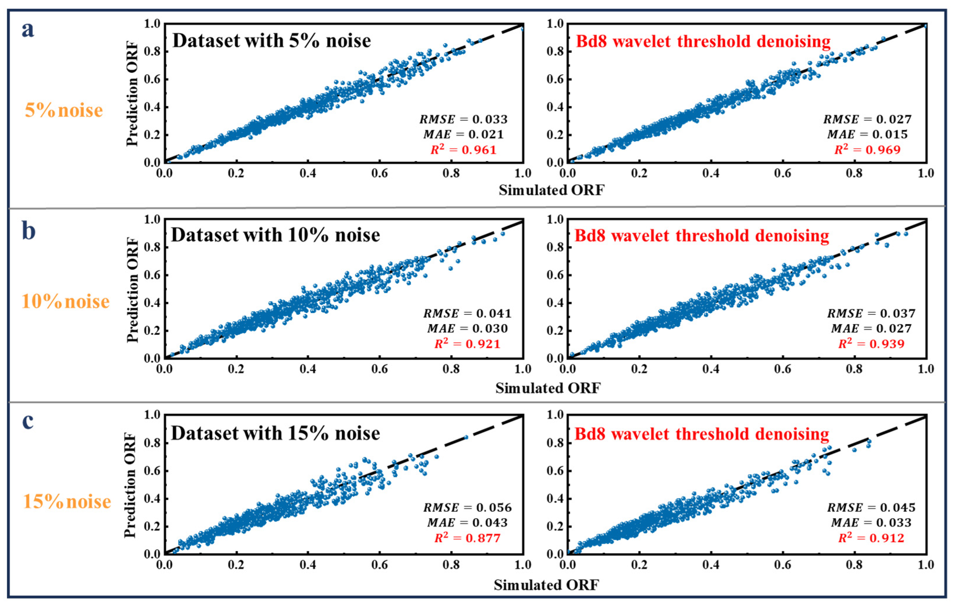
Figure 10 provides a comparative analysis of test set prediction results before and after denoising the dataset. Utilizing the Bd8 wavelet for denoising brought the predicted and simulated ORF data points in the cross-plot closer to the fit line (slope = 1), signifying an improvement in the model’s predictive accuracy.

In Figure 10a, the dataset with a 5% noise level displays a slight enhancement in prediction accuracy post-denoising. The R² value increases by a mere 0.08, while both RMSE and MAE decrease by 0.06. In contrast, Figure 10c highlights that the dataset with 15% noise sees a notable uptick in prediction accuracy after denoising: R² rises by 0.35 and RMSE and MAE drop by 0.011 and 0.010, respectively. A key observation from Figure 10 is that wavelet denoising appears more beneficial for datasets with pronounced noise levels. For datasets with minimal noise, the impact of denoising is subdued. This phenomenon can be linked to the LightGBM model’s inherent resilience to noise, as it retains high predictive accuracy (R² > 0.96), even when faced with an added 5% noise. However, for datasets with low noise, denoising could inadvertently strip away valuable information that might seem noisy, potentially compromising the model’s predictive capability.

3.4. Screening and Evaluation of Main Control Factors

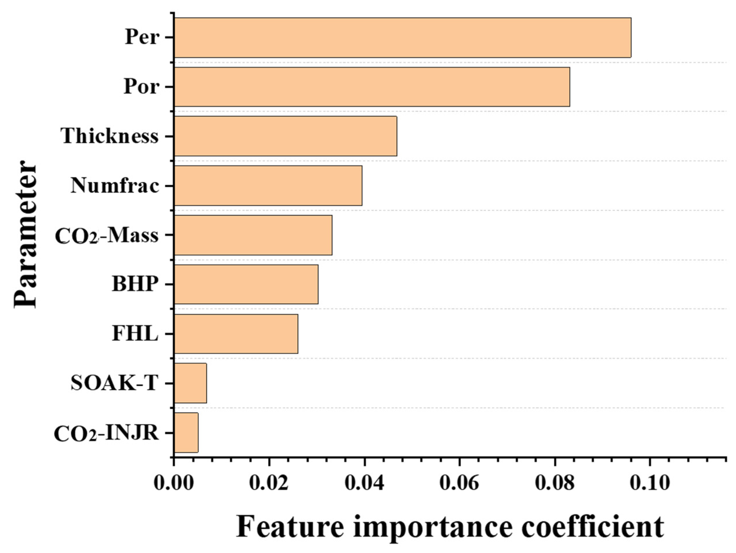
Figure 11 presents the ranking results based on the feature selection method of the LightGBM model. LightGBM ranks each feature based on both average information gain and total information gain, resulting in a comprehensive ranking of influential factors. As evident from Figure 11, permeability stands out as the most influential factor, ranking first. Porosity and reservoir thickness are also significantly affected, ranking second and third, respectively. Following these, the factors of fracture count, CO₂ mass, BHP, half-length of fracture, soak time, and carbon dioxide injection rate are less influential.

Permeability, porosity, reservoir pressure, and permeability have long been used as screening criteria for evaluating CO₂-EOR. In this study, we incorporated CO₂ accumulation, injection rate, and soak time to investigate the impact of these factors on the CO₂ flooding efficiency. Although CO₂ has a significant diluting effect and can theoretically enhance oil recovery to a greater extent, as seen in Figure 11, the influence of CO₂ accumulation on the injection volume only ranks fifth. This suggests that the effectiveness of CO₂ flooding is significantly influenced by permeability and porosity. For low-permeability and tight reservoirs, conducting CO₂-EOR operations may require a screening of the reservoir conditions.

4. Conclusions

This article introduces a novel approach for the rapid and precise prediction of recovery in CO₂ flooding operations within tight oil reservoirs through the use of ML models. By conducting thorough data mining on the collected data, this study develops an ML model specifically tailored for assessing CO₂ flooding efficiency in such reservoirs. The key findings are summarized as follows:

(1)

By considering actual blocks as examples, a numerical simulation model for CO₂ flooding in low-permeability tight oil reservoirs has been developed. Utilizing the Latin hypercube design method, a comprehensive dataset comprising 4090 numerical simulations is generated, providing a robust foundation for the ML model to analyze ORF.

(2)

The study examines the impact of introducing varying levels of noise (5%, 10%, and 15%) to the simulation data on the predictive accuracy of LightGBM, XGBoost, and RF models regarding ORF. Findings reveal that the LightGBM model outperforms the others, demonstrating superior predictive capabilities for CO₂ flooding recovery efficiency in tight oil reservoirs, with R² values of 0.995, 0.961, 0.921, and 0.877 for the original, 5% noise, 10% noise, and 15% noise datasets, respectively.

(3)

This research identifies the primary factors influencing CO₂-enhanced oil recovery, ranked as follows: permeability, porosity, reservoir thickness, number of fracturing fractures, CO₂ mass, BHP, fracture half-length, soak time, and CO₂ injection rate.

(4)

The method proposed here stands as a promising alternative to conventional CO₂-ORF prediction techniques. Embracing ML for supplementary decision making offers a more adaptable and accurate framework for evaluations, reducing the risk of misjudgments associated with static indicator ranges.

Employing ML as proxies for predicting recovery presents distinct challenges. To guarantee the universality of the models, extensive and high-quality geological and production data from diverse reservoirs are essential for training. Moreover, the increased volume and complexity of data necessitate substantial investment in rapidly optimizing model parameters to boost accuracy.

Moving forward, our focus will shift to analyzing the impact of various petroleum component parameters on CO₂ flooding. It aims to refine our model’s adaptability and to elevate the precision of CO₂-EOR predictions across diverse reservoir conditions. Furthermore, the model will be applied to some actual reservoirs. This expansion entails blending geological and production data from actual reservoirs with simulated datasets, then conducting preprocessing on this amalgamated dataset. Training the model with this refined data will verify its feasibility in real-world conditions.

References

1. Vo Thanh, H.; Sheini Dashtgoli, D.; Zhang, H.; Min, B. Machine-learning-based prediction of oil recovery factor for experimental CO2-Foam chemical EOR: Implications for carbon utilization projects. Energy 2023, 278, 127860. [Google Scholar] [CrossRef]
2. Farajzadeh, R.; Eftekhari, A.A.; Dafnomilis, G.; Lake, L.W.; Bruining, J. On the sustainability of CO2 storage through CO2—Enhanced oil recovery. Appl. Energy 2020, 261, 114467. [Google Scholar] [CrossRef]
3. Zuloaga-Molero, P.; Yu, W.; Xu, Y.; Sepehrnoori, K.; Li, B. Simulation Study of CO2-EOR in Tight Oil Reservoirs with Complex Fracture Geometries. Sci. Rep. 2016, 6, 33445. [Google Scholar] [CrossRef] [PubMed]
4. Chen, T.; Song, L.; Zhang, X.; Yang, Y.; Fan, H.; Pan, B. A Review of Mineral and Rock Wettability Changes Induced by Reaction: Implications for CO2 Storage in Saline Reservoirs. Energies 2023, 16, 3484. [Google Scholar] [CrossRef]
5. Bello, A.; Ivanova, A.; Cheremisin, A. A Comprehensive Review of the Role of CO2 Foam EOR in the Reduction of Carbon Footprint in the Petroleum Industry. Energies 2023, 16, 1167. [Google Scholar] [CrossRef]
6. Zhang, J.; Tian, L. Tight oil recovery prediction based on extreme gradient boosting algorithm and support vector regression algorithm variable weight combination model. Sci. Technol. Eng. 2022, 22, 4778–4787. [Google Scholar]
7. Sun, R.; Pu, H.; Yu, W.; Miao, J.; Zhao, J.X. Simulation-based enhanced oil recovery predictions from wettability alteration in the Middle Bakken tight reservoir with hydraulic fractures. Fuel 2019, 253, 229–237. [Google Scholar] [CrossRef]
8. Miura, K.; Wang, J. An Analytical Model to Predict Cumulative Steam Oil Ratio (CSOR) in Thermal Recovery SAGD Process. In Proceedings of the Canadian Unconventional Resources and International Petroleum Conference, Calgary, AB, Canada, 19–21 October 2010; p. 137604. [Google Scholar]
9. Teng, L.; Zhang, D.; Li, Y.; Wang, W.; Wang, L.; Hu, Q.; Ye, X.; Bian, J.; Teng, W. Multiphase mixture model to predict temperature drop in highly choked conditions in CO2 enhanced oil recovery. Appl. Therm. Eng. 2016, 108, 670–679. [Google Scholar] [CrossRef]
10. Guo, C.; Li, H.; Tao, Y.; Lang, L.; Niu, Z. Water invasion and remaining gas distribution in carbonate gas reservoirs using core displacement and NMR. J. Cent. South Univ. 2020, 27, 531–541. [Google Scholar] [CrossRef]
11. Al-Jifri, M.; Al-Attar, H.; Boukadi, F. New proxy models for predicting oil recovery factor in waterflooded heterogeneous reservoirs. J. Pet. Explor. Prod. 2021, 11, 1443–1459. [Google Scholar] [CrossRef]
12. Fathaddin, M.T.; Thomas, M.M.; Pasarai, U. Predicting oil recovery through CO2 flooding simulation using methods of continuous and water alternating gas. J. Phys. Conf. Ser. 2019, 1402, 55015. [Google Scholar] [CrossRef]
13. Yuan, Z.; Wang, J.; Li, S.; Ren, J.; Zhou, M. A new approach to estimating recovery factor for extra-low permeability water-flooding sandstone reservoirs. Pet. Explor. Dev. 2014, 41, 377–386. [Google Scholar] [CrossRef]
14. Yue, M.; Song, T.; Chen, Q.; Yu, M.; Wang, Y.; Wang, J.; Du, S.; Song, H. Prediction of effective stimulated reservoir volume after hydraulic fracturing utilizing deep learning. Pet. Sci. Technol. 2023, 41, 1934–1956. [Google Scholar] [CrossRef]
15. Huang, J.; Wang, H. Pore-Scale Simulation of Confined Phase Behavior with Pore Size Distribution and Its Effects on Shale Oil Production. Energies 2021, 14, 1315. [Google Scholar] [CrossRef]
16. Sun, H.; Wang, H.; Zhu, S.; Nie, H.; Liu, Y.; Li, Y.; Li, S.; Cao, W.; Chang, B. Reserve evaluation of high pressure and ultra-high-pressure reservoirs with power function material balance method. Nat. Gas Ind. B 2019, 6, 509–516. [Google Scholar] [CrossRef]
17. Cheng, M.; Lei, G.; Gao, J.; Xia, T.; Wang, H. Laboratory Experiment, Production Performance Prediction Model, and Field Application of Multi-slug Microbial Enhanced Oil Recovery. Energy Fuels 2014, 28, 6655–6665. [Google Scholar] [CrossRef]
18. Hadia, N.; Chaudhari, L.; Aggarwal, A.; Mitra, S.K.; Vinjamur, M.; Singh, R. Experimental and numerical investigation of one-dimensional waterflood in porous reservoir. Exp. Therm. Fluid Sci. 2007, 32, 355–361. [Google Scholar] [CrossRef]
19. Zhong, Q.; Shi, Y.; Liu, P.; Peng, B.; Zhuang, Y. Study on injecting time of CO2 flooding in low permeability reservoir. Fault-Block Oil Gas Field 2012, 19, 346–349. [Google Scholar]
20. Al-qaness, M.A.A.; Ewees, A.A.; Thanh, H.V.; AlRassas, A.M.; Dahou, A.; Elaziz, M.A. Predicting CO2 trapping in deep saline aquifers using optimized long short-term memory. Environ. Sci. Pollut. Res. 2023, 30, 33780–33794. [Google Scholar] [CrossRef]
21. Esmaili, S.; Mohaghegh, S.D. Full field reservoir modeling of shale assets using advanced data-driven analytics. Geosci. Front. 2016, 7, 11–20. [Google Scholar] [CrossRef]
22. Miah, M.I.; Ahmed, S.; Zendehboudi, S. Connectionist and mutual information tools to determine water saturation and rank input log variables. J. Pet. Sci. Eng. 2020, 190, 106741. [Google Scholar] [CrossRef]
23. Yasin, Q.; Sohail, G.M.; Ding, Y.; Ismail, A.; Du, Q. Estimation of Petrophysical Parameters from Seismic Inversion by Combining Particle Swarm Optimization and Multilayer Linear Calculator. Nat. Resour. Res. 2020, 29, 3291–3317. [Google Scholar] [CrossRef]
24. Muojeke, S.; Venkatesan, R.; Khan, F. Supervised data-driven approach to early kick detection during drilling operation. J. Pet. Sci. Eng. 2020, 192, 107324. [Google Scholar] [CrossRef]
25. Hegde, C.; Pyrcz, M.; Millwater, H.; Daigle, H.; Gray, K. Fully coupled end-to-end drilling optimization model using machine learning. J. Pet. Sci. Eng. 2020, 186, 106681. [Google Scholar] [CrossRef]
26. Gurina, E.; Klyuchnikov, N.; Zaytsev, A.; Romanenkova, E.; Antipova, K.; Simon, I.; Makarov, V.; Koroteev, D. Application of machine learning to accidents detection at directional drilling. J. Pet. Sci. Eng. 2020, 184, 106519. [Google Scholar] [CrossRef]
27. Zhu, W.; Song, T.; Wang, M.; Jin, W.; Song, H.; Yue, M. Stratigraphic subdivision-based logging curves generation using neural random forests. J. Pet. Sci. Eng. 2022, 219, 111086. [Google Scholar] [CrossRef]
28. Gupta, S.; Fuehrer, F.; Jeyachandra, B.C. In Production Forecasting in Unconventional Resources using Data Mining and Time Series Analysis. In Proceedings of the SPE/CSUR Unconventional Resources Conference, Calgary, AB, Canada, 30 September–2 October 2014. [Google Scholar]
29. Lala, A.M.S.; Lala, H.M.S. Study on the improving method for gas production prediction in tight clastic reservoir. Arab. J. Geosci. 2017, 10, 70. [Google Scholar] [CrossRef]
30. Lin, B.; Guo, J.; Liu, X.; Xiang, J.; Zhong, H. Prediction of flowback ratio and production in Sichuan shale gas reservoirs and their relationships with stimulated reservoir volume. J. Pet. Sci. Eng. 2020, 184, 106529. [Google Scholar] [CrossRef]
31. Liu, W.; Yang, Y.; Qiao, C.; Liu, C.; Lian, B.; Yuan, Q. Progress of Seepage Law and Development Technologies for Shale Condensate Gas Reservoirs. Energies 2023, 16, 2446. [Google Scholar] [CrossRef]
32. Al-Mudhafar, W.J. Integrating lithofacies and well logging data into smooth generalized additive model for improved permeability estimation: Zubair formation, South Rumaila oil field. Mar. Geophys. Res. 2019, 40, 315–332. [Google Scholar] [CrossRef]
33. Al-Mudhafar, W.J. Integrating machine learning and data analytics for geostatistical characterization of clastic reservoirs. J. Pet. Sci. Eng. 2020, 195, 107837. [Google Scholar] [CrossRef]
34. Pan, B.; Song, T.; Yue, M.; Chen, S.; Zhang, L.; Edlmann, K.; Neil, C.W.; Zhu, W.; Iglauer, S. Machine learning–based shale wettability prediction: Implications for H2, CH4 and CO2 geo-storage. Int. J. Hydrogen Energy 2024, 56, 1384–1390. [Google Scholar] [CrossRef]
35. Van, S.L.; Chon, B.H. Effective Prediction and Management of a CO2 Flooding Process for Enhancing Oil Recovery Using Artificial Neural Networks. J. Energy Resour. Technol. 2017, 140, 032906. [Google Scholar] [CrossRef]
36. Cheraghi, Y.; Kord, S.; Mashayekhizadeh, V. Application of machine learning techniques for selecting the most suitable enhanced oil recovery method; challenges and opportunities. J. Pet. Sci. Eng. 2021, 205, 108761. [Google Scholar] [CrossRef]
37. Esene, C.; Zendehboudi, S.; Shiri, H.; Aborig, A. Deterministic tools to predict recovery performance of carbonated water injection. J. Mol. Liq. 2020, 301, 111911. [Google Scholar] [CrossRef]
38. Pan, S.; Zheng, Z.; Guo, Z.; Luo, H. An optimized XGBoost method for predicting reservoir porosity using petrophysical logs. J. Pet. Sci. Eng. 2022, 208, 109520. [Google Scholar] [CrossRef]
39. Huang, Z.; Chen, Z. Comparison of different machine learning algorithms for predicting the SAGD production performance. J. Pet. Sci. Eng. 2021, 202, 108559. [Google Scholar] [CrossRef]
40. Shen, B.; Yang, S.; Gao, X.; Li, S.; Ren, S.; Chen, H. A novel CO2-EOR potential evaluation method based on BO-LightGBM algorithms using hybrid feature mining. Geoenergy Sci. Eng. 2023, 222, 211427. [Google Scholar] [CrossRef]
41. Taber, J.J.; Martin, F.D.; Seright, R.S. EOR Screening Criteria Revisited—Part 1: Introduction to Screening Criteria and Enhanced Recovery Field Projects. Spe Reserv. Eng. 1997, 12, 189–198. [Google Scholar] [CrossRef]
42. Lee, J.H.; Park, Y.C.; Sung, W.M.; Lee, Y.S. A Simulation of a Trap Mechanism for the Sequestration of CO2 into Gorae V Aquifer, Korea. Energy Sources Part A Recovery Util. Environ. Eff. 2010, 32, 796–808. [Google Scholar]
43. Liu, B.; Zhang, Y. CO2 Modeling in a Deep Saline Aquifer: A Predictive Uncertainty Analysis Using Design of Experiment. Environ. Sci. Technol. 2011, 45, 3504–3510. [Google Scholar] [CrossRef] [PubMed]
44. Abbaszadeh, M.; Shariatipour, S.M. Investigating the Impact of Reservoir Properties and Injection Parameters on Carbon Dioxide Dissolution in Saline Aquifers. Fluids 2018, 3, 76. [Google Scholar] [CrossRef]
45. Gao, M.; Liu, Z.; Qian, S.; Liu, W.; Li, W.; Yin, H.; Cao, J. Machine-Learning-Based Approach to Optimize CO2-WAG Flooding in Low Permeability Oil Reservoirs. Energies 2023, 16, 6149. [Google Scholar] [CrossRef]
46. Li, S.; Wang, Z.; Kang, Y.; Hou, J. Noise reduction of a safety valve pressure relief signal based on an improved wavelet threshold function. J. Vib. Shock. 2021, 40, 143–150. [Google Scholar]
47. Li, W.; Xu, W.; Zhang, T. Improvement of Threshold Denoising Method Based on Wavelet Transform. Comput. Simul. 2021, 38, 348–351. [Google Scholar]
48. Song, T.; Zhu, W.; Chen, Z.; Jin, W.; Song, H.; Fan, L.; Yue, M. A novel well-logging data generation model integrated with random forests and adaptive domain clustering algorithms. Geoenergy Sci. Eng. 2023, 231, 212381. [Google Scholar] [CrossRef]
49. Liaw, A.; Wiener, M. Classification and regression by randomForest. R News 2002, 2, 18–22. [Google Scholar]
50. Vo Thanh, H.; Lee, K. Application of machine learning to predict CO2 trapping performance in deep saline aquifers. Energy 2022, 239, 122457. [Google Scholar] [CrossRef]
51. Vo Thanh, H.; Yasin, Q.; Al-Mudhafar, W.J.; Lee, K. Knowledge-based machine learning techniques for accurate prediction of CO2 storage performance in underground saline aquifers. Appl. Energy 2022, 314, 118985. [Google Scholar] [CrossRef]
52. Meng, M.; Zhong, R.; Wei, Z. Prediction of methane adsorption in shale: Classical models and machine learning based models. Fuel 2020, 278, 118358. [Google Scholar] [CrossRef]
53. Gholami, H.; Mohamadifar, A.; Collins, A.L. Spatial mapping of the provenance of storm dust: Application of data mining and ensemble modelling. Atmos. Res. 2020, 233, 104716. [Google Scholar] [CrossRef]
54. Ke, G.; Meng, Q.; Finley, T.; Wang, T.; Chen, W.; Ma, W.; Ye, Q.; Liu, T.Y. Lightgbm: A highly efficient gradient boosting decision tree. Adv. Neural Inf. Process. Syst. 2017, 30, 1–2. [Google Scholar]
55. Stazio, A.; Victores, J.G.; Estevez, D.; Balaguer, C. A Study on Machine Vision Techniques for the Inspection of Health Personnels’ Protective Suits for the Treatment of Patients in Extreme Isolation. Electronics 2019, 8, 743. [Google Scholar] [CrossRef]
Figure 1. Workflow of ORF prediction using three ML models.
Energies 17 01303 g001
Figure 2. CMG reservoir geological model.
Energies 17 01303 g002
Figure 3. Oil–water relative permeability curves.
Energies 17 01303 g003
Figure 4. The integrated process Petrel and CMOST optimizer for considering geological realizations to generate the training samples.
Energies 17 01303 g004
Figure 5. The comparison of data with 15% noise before and after denoising.
Energies 17 01303 g005
Figure 6. The architecture of LightGBM.
Energies 17 01303 g006
Figure 7. Schematic diagram of random search method.
Energies 17 01303 g007
Figure 8. Cross correlation between ORF predicted by LightGBM model and ORF obtained from numerical simulation under different noise levels (a) prediction result of original dataset (b) prediction result at the 5% noise level (c) prediction result at the 10% noise level (d) prediction result at the 15% noise level.
Energies 17 01303 g008
Figure 9. The statistical performance of the ML models under different noise levels: (a) R2, (b) RMSE, and (c) MAE.
Energies 17 01303 g009
Figure 10. The statistical performance of the LightGBM model under different noise levels: (a) R2, (b) RMSE, and (c) MAE.
Energies 17 01303 g010
Figure 11. Ranking of feature importance.
Energies 17 01303 g011