Article

Position Sensorless Vector Control System for Lawnmower Permanent Magnet Synchronous Motor Based on Extended Kalman Filter

1
School of Mechanical Engineering, Qilu University of Technology (Shandong Academy of Sciences), Jinan 250300, China
2
School of Electronics and Information, Aerospace Information Technology University, Jinan 250200, China
3
School of Information and Automation Engineering, Qilu University of Technology (Shandong Academy of Sciences), Jinan 250300, China
*
Author to whom correspondence should be addressed.
Energies 2024, 17(5), 1230; https://doi.org/10.3390/en17051230
Submission received: 14 February 2024 / Revised: 23 February 2024 / Accepted: 29 February 2024 / Published: 4 March 2024
(This article belongs to the Section F: Electrical Engineering)

Abstract

:
In this paper, we describe a position sensorless vector control system for a permanent magnet synchronous motor (PMSM) for a lawnmower in order to solve the problems of inferior dynamic performance and insufficient load resistance in the control process of lawnmower motors. A speed–current double-closed-loop vector control strategy was adopted to control the motor speed; an extended Kalman filter (EKF) was constructed to track the motor rotor position. STM32F407 was selected as the main control chip to establish the hardware experimental platform, and the performance of the control system was evaluated. The experimental results demonstrate that the control system accurately regulates motor speed, has good dynamic response characteristics, and can maintain stability under various loads; therefore, it meets the performance requirements of lawnmower motors in practical operation.

1. Introduction

With today’s accelerated urbanization, lawn maintenance and mowing have become important parts of urban and rural greening, for which lawnmowers provide essential support [1,2,3]. The typical working conditions of lawnmowers mainly involve the process of mowing the lawn under a changing lawn density; that is, the changes in the load can be divided into two categories of working conditions: the first is when the density in the working area of the lawn changes gently and the distribution of vegetation growth is uniform; the second is when the density in the working area of the lawn chaotically changes and the distribution of vegetation growth is not uniform [4]. In order for a lawnmower to be able to cope with working scenarios with different turf densities, it is therefore essential to implement an efficient control strategy for the lawnmower [5].
The control of a lawnmower is mainly determined by the control of the lawnmower motor [6]. The capacity of the motor control system directly determines the efficiency of the lawnmower, the quality of operation, and the user experience [7]; therefore, the selection of the type of motor for the lawnmower as well as the selection of the corresponding control strategy are particularly important [8]. Permanent magnet synchronous motors (PMSMs) have a simple structure, high power factor, high torque-to-current ratio, high efficiency, low noise, and long service life [9] and have been increasingly widely used in high-performance systems such as numerical control and robotics [10,11,12]. Using a PMSM as a lawnmower motor can effectively reduce the maintenance and output costs of the machine [13] and improve the control performance and service life of the mower, so it is the ideal choice for a lawnmower motor [14]. Vector control methods applicable to PMSMs usually require the installation of position sensors, but the use of sensors raises the cost and increases the volume of the motor, and sensor lines are susceptible to environmental disturbances, leading to an unstable control system [15]. Therefore, a sensorless position control strategy is particularly important [16].
At present, sensorless position control technology in PMSMs is gradually being implemented [17] and can be predominantly divided into two aspects: the first concerns PMSMs operating at zero and low speeds, and the second pertains to PMSMs operating at medium and high speeds [18]. In low-speed control technology, a high-frequency injection method involves injecting high-frequency voltage signals or current signals into the motor shaft system. At that point, the rotor position information is contained in the current (or voltage) response signals of the corresponding phases [19]. By carrying out special signal processing on the response signals, the rotor position and speed information can be extracted; this does not rely on the EMF signals of the motor and is suitable for estimating the rotor position and speed in the low-speed phase. However, the need to inject high-frequency signals into various phases of the motor may lead to problems such as electromagnetic torque fluctuation, high-frequency vibration and noise, and power loss [20]. The I/F control method is a type of inverter speed control process that ensures there is stable current through the current closed loop in order to prevent it from being too large or too small [21]. I/F control can directly control the torque current, enhancing the motor’s torque output and load torque adjustment capability while eradicating low-frequency oscillation during the motor’s operation process. However, it also results in the motor’s current amplitude being fixed and the loss of the current’s ability to follow the load’s self-adjustment [22]. In medium- and high-speed control, there are two types of methods: open loop and closed loop. In the open-loop method, the direct calculation method is based on a motor model formula and the constraints for the extreme values of the d- and q-axes’ current command value of weak magnetism; although the operation is simple, the method relies heavily on the motor parameters. Parameter error therefore very easily affects the control performance [23]. The back electromotive force (BEMF) approach is straightforward, but when the motor is operating at low speed or is stationary, the back electromotive force signal is very weak and needs to be processed, which results in a phase shift in the signal [24]. In the closed-loop method, sliding mode variable structure control has the benefits of rapid response and high robustness, but the high-frequency switching causes large system jitter [25]. The model-referenced adaptive method does not require an exact mathematical model [26], but it is cumbersome to operate, and the control system is sophisticated [27]. Common state observer methods include the sliding mode observer and the extended Kalman filter [28], among others. The sliding mode observer method can solve the problem of motors that are difficult to control at high speeds and under heavy loads with high robustness, but it requires a lot of operations [29]. The extended Kalman filter (EKF) can effectively reduce the impact of random interference and measurement noise [30] and can quickly track the actual state of the system; also, the extended Kalman filter takes into account the impact of interference and measurement error [31], so it has a strong adaptive ability to parameter changes and external interference. The disadvantage is that it is computationally intensive to operate and has certain processor requirements [32].
By synthesizing the above analysis, we can conclude that the theoretical approach to PMSMs is relatively mature. However, in reality, the application of control theory to actual industrial and agricultural equipment still requires a lot of work and testing [33]. Based on the performance requirements of a lawnmower in practical work, the researchers of this study selected a PMSM with a power of 500W as a control object, built a hardware control platform around it, established an estimation model for motor speed and rotor position based on the extended Kalman filter, and designed a sensorless PMSM vector control system for a lawnmower.
The contributions of this study include the following:
1.
A sensorless position vector control system based on the EKF was designed for a specifically powered lawnmower PMSM.
2.
To evaluate the performance of the control system, experiments with no load, acceleration, deceleration, and different loads as well as simulated typical lawnmower working conditions were designed; these verified the control system’s robustness and performance.
3.
In this study, a vector control system based on the EKF was successfully applied to a lawnmower motor and achieved stable and efficient control, providing practical experience and data support for the field of lawnmower motor control.

2. Mathematical Model of Permanent Magnet Synchronous Motors

PMSMs have become one of the first choices for lawnmower motors due to their high efficiency, high power density, and fast response, but since PMSMs are nonlinear, multivariable, and highly coupled complex systems, it is difficult to implement control strategies. A method of mathematical modeling of the motor to provide an accurate description of the motor state is key to the development of efficient control strategies, so a thorough analysis of the mathematical model of a PMSM is required before designing the motor control system.
The voltage equation of a PMSM in the stationary coordinate system’s α β axis is as follows:
u α = R i α + L s ( d i α ) / d t ω e ψ f sin θ e u β = R i β + L s ( d i β ) / d t ω e ψ f sin θ e
Transforming Equation (1) into the current equation gives the following:
( d i α ) / d t = R / L s i α + ω e ( ψ f / L s ) sin θ e + u α / L s ( d i β ) / d t = R / L s i β ω e ( ψ f / L s ) cos θ e + u α / L s
In Equation (2), i α and u α are the current and voltage, respectively, in the α -axis, i β and u β are the current and voltage, respectively, in the β -axis, R is the stator phase resistance, L s is the stator phase inductance, ω e is the electrical angular velocity of the rotor, θ e is the rotor position, and ψ f is the permanent magnet chain. The voltages u α and u β and the currents i α and i β can be obtained by measurement.
Considering that the mechanical time constant of a PMSM is much larger than the electrical time constant, it can be assumed in the calculation process that the motor speed ω e is constant during each sampling period, and the following equation can be obtained:
( d ω e ) / d t = 0 ( d θ e ) / d t = ω e
Taking i α , i β , ω e , and θ e as system states and u α and u β as input variables, the following equation of state can be obtained:
x ˙ = d x / d t = f ( x ) + B u
y = H x
where the variables are as follows:
x = i α i β ω e θ e , u = u α u β , y = i α i β
f ( x ) = R i α / L s + ω e ( ψ f / L s ) sin θ e R i β / L s ω e ( ψ f / L s ) cos θ e 0 ω e
B = 1 / L s 0 0 1 / L s 0 0 0 0 , H = 1 0 0 0 0 1 0 0
Since Equations (4) and (5) are both nonlinear, they need to be linearized, and their discretized mathematical model can be expressed as follows:
x ( k + 1 ) = f [ x ( k ) ] + B ( k ) u ( k ) + W ( k )
y ( k ) = H ( k ) x ( k ) + V ( k )
In the above equation, W ( k ) denotes the state noise and V ( k ) denotes the measurement noise. Supposing that both W ( k ) and V ( k ) are Gaussian white noise with zero mean, it follows that:
E W ( k ) = 0 , E V ( k ) = 0
In the above equation, E represents the mathematical expectation.
In the extended Kalman filter algorithm, neither the noise vectors W nor V will be used directly, but the respective covariance matrices Q and R will, where Q and R are defined, respectively, as follows:
cos ( V ) = E V V T = Q cos ( W ) = E W W T = R
In the above equations, it is supposed that W ( k ) and V ( k ) are independent and that x ( 0 ) is a vector that is random and is independent of W ( k ) and V ( k ) .

3. Sensorless Vector Control System for Permanent Magnet Synchronous Motors

3.1. Implementation of the Extended Kalman Filter

The state observation process of the EKF is divided into a prediction phase and a correction phase as follows:
1.
Estimating the state vector: based on the state estimate x ^ ( k ) at the previous moment and the input value u ( k ) , estimating the state vector at the next moment ( k + 1 ) can be undertaken using the following expression:
x ^ ( k + 1 ) = x ˜ ( k ) + T s [ f ( x ^ ( k ) ) + B ( k ) u ( k ) ]
where T s denotes the sampling period, x ^ denotes the state estimate, and x ˜ denotes the prediction.
2.
Then, the corresponding output y ˜ ( k + 1 ) can be computed to obtain the following:
y ˜ ( k + 1 ) = H x ˜ ( k + 1 )
In this step, the EKF algorithm predicts the measured value y ˜ ( k + 1 ) at the next moment ( k + 1 ) based on the predicted value x ˜ ( k + 1 ) of the state and, thus, uses this predicted value in the update step to update the state estimate.
3.
The error covariance matrix can then be computed to obtain the following:
p ˜ ( k + 1 ) = p ^ ( k ) + T s [ F ( k ) p ^ ( k ) + p ^ ( k ) F T ( k ) ] + Q
The process noise covariance matrix Q describes the uncertainty and noise in the system dynamics, which are usually estimated based on empirical knowledge from system models and practical applications.
When F ( k ) has the following expression,
F ( k ) = ( x ) x x = x ^ ( k ) ,
the following results are obtained:
F ( k ) = R / L s 0 ( ψ f / L s ) sin θ ^ e ( k ) ω ^ e ( k ) ( ψ f / L s ) cos θ ^ e ( k ) 0 R / L s ( ψ f / L s ) cos θ ^ e ( k ) ω ^ e ( k ) ( ψ f / L s ) sin θ ^ e ( k ) 0 0 0 0 0 0 1 0
4.
The gain matrix K ( k + 1 ) of the EKF is computed and obtained as follows:
K ( k + 1 ) = p ˜ ( k + 1 ) H T [ H p ˜ ( k + 1 ) H T + R ] 1
The gain matrix K ( k + 1 ) is used to measure the difference between the predicted value and the actual measurement and to correct the state estimate based on this difference.
5.
The feedback correction of the predicted state vector x ˜ ( k + 1 ) results in the optimized state estimate x ˜ ( k + 1 ) as follows:
x ˜ ( k + 1 ) = x ˜ ( k + 1 ) + K ( k + 1 ) [ y ( k + 1 ) y ˜ ( k + 1 ) ]
This stage is the corrected prediction, which is designed to correct the predicted state values to more closely match the actual observations. In this stage, the previously predicted states are compared with the actual observations, and the observations are used to correct the state estimates and to make them more accurate. In the equation, y ( k + 1 ) represents the observed value used to correct the state estimate at the moment ( k + 1 ) . Usually, the observed value can be measured by the detection equipment, and in this paper, according to Equation (5), y ( k + 1 ) represents the current value at the moment ( k + 1 ) , which is specifically collected by the hardware sampling circuit and converted by the processing program.
6.
The covariance matrix of the estimation error needs to be pre-calculated for the next estimation as follows:
p ^ ( k + 1 ) = p ˜ ( k + 1 ) = K ( k + 1 ) H p ˜ ( k + 1 )
The above implementation process is based on the extended Kalman filter, the main concept of which is that feedback adjustment through the observation results can optimize the control system, remove the influence of uncertainty, and ultimately realize accurate estimation of the state.
As shown in Figure 1, the EKF works by correcting the state quantities of the state observer using the difference between the output of the observer and the actual output of the system multiplied by a Kalman gain, K, as the correction value of the observer and also by adaptively adjusting the Kalman gain, K, according to the error covariance.
In the motor control system developed in this paper, the EKF is used to observe the motor rotational speed and rotor position information: specifically, by using the motor control system to easily collect the motor terminal voltage, current, and other signals; constructing the motor state equations applicable to the EKF; and using the EKF to estimate the parameters of the motor control system online so as to obtain the motor speed as well as the rotor position information.
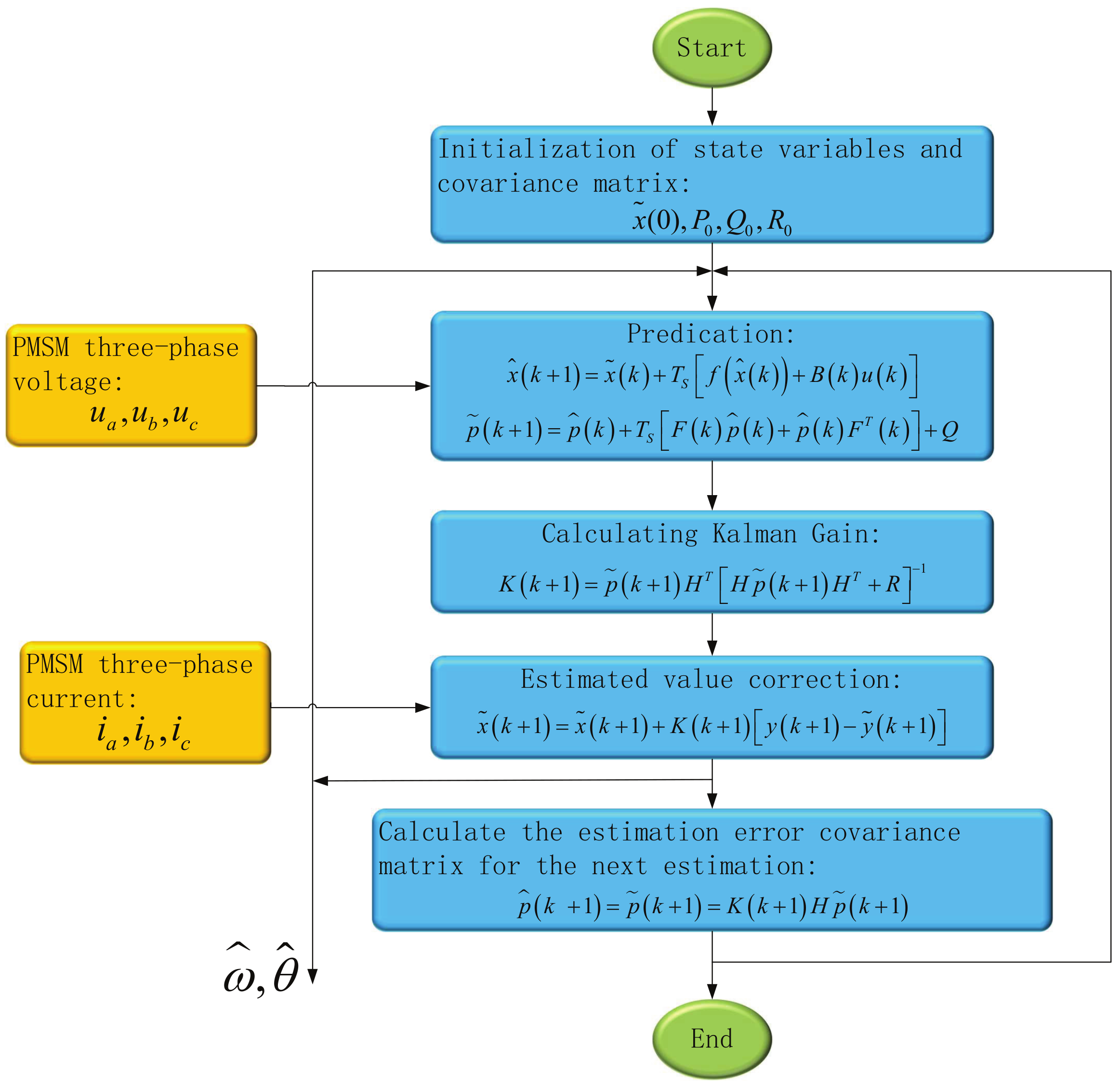
The flowchart of the EKF algorithm for a PMSM is shown in Figure 2.
As shown in Figure 2, during the execution of the EKF algorithm, the input variables are the three-phase voltage signals, u a , u b , and u c , and the three-phase current signals, i a , i b , and i c , of the PMSM, which are captured by hardware sampling circuits and input into the EKF algorithm after analog-to-digital (AD) conversion. The output signals of the EKF algorithm are the estimated motor speed ω ^ and the motor rotor position information θ ^ . As the position information of the motor rotor is obtained by the EKF algorithm, an additional position sensor is no longer required, allowing PMSM control without a position sensor.

3.2. Vector Control Strategy Based on the Extended Kalman Filter

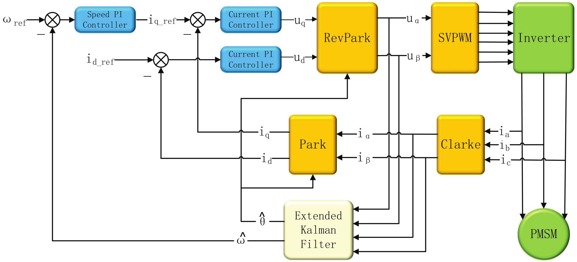
The vector control strategy of i d _ r e f = 0 is adopted to establish a sensorless vector control system for PMSM based on EKF, and the control block diagram is shown in Figure 3. Firstly, the current signals, i a , i b , and i c , of the motor are collected, and, after Clarke and Park transformations, the feedback signals i d and i q are obtained, which are compared with the set reference current signals i d _ r e f and i q _ r e f . The control voltages, u d and u q , in the d q coordinate system are obtained by the PI regulator, and they are then transformed to u α and u β in the α β coordinate system using a RevPark transformation; finally, the switching states of six MOS tubes are obtained by u α and u β through a space vector pulse width modulation (SVPWM) module in order to realize control of the PMSM. The EKF is used in the control process to obtain the rotational speed and position information of the motor. The inputs of the EKF are the currents i α and i β and the voltages u α and u β of the motor in the two-phase stationary coordinate system, and the outputs are the rotor position information θ ^ and the motor rotational speed ω ^ . Through the above control method, closed-loop control effect is achieved, which ensures the stability of the system.
In terms of programming, the PMSM sensorless vector control system designed in this paper is divided into two modules: the control module and the observation module. The control module is used to send control signals to the motor, and the observation module is used to obtain the rotor position information and provide it to the control module. According to Figure 3, it is derived that the execution speed of the observer must be faster than that of the controller in order to achieve effective and accurate control. separate design of the observation module and the control module in the control system maintains their independence and reduces the coupling between them, which helps to simplify the system design and development process and improves the maintainability and scalability of the system.

4. Experimentation

4.1. Simulation Results

The extended-Kalman-filter-based PMSM control system was built using Simulink in MATLAB R2018b, and simulation experiments were conducted to verify the performance of the proposed extended Kalman filter algorithm and to observe the control effect. The simulated PMSM parameters were set as listed in Table 1.
In simulation experiments, after trial attempts, the parameters P 0 , Q, and R were set as follows:
P 0 = 1 0 0 0 0 1 0 0 0 0 1 0 0 0 0 1 , Q = 0.1 0 0 0 0 0.1 0 0 0 0 0.1 0 0 0 0 0.01 , R = 0.2 0 0 0.2
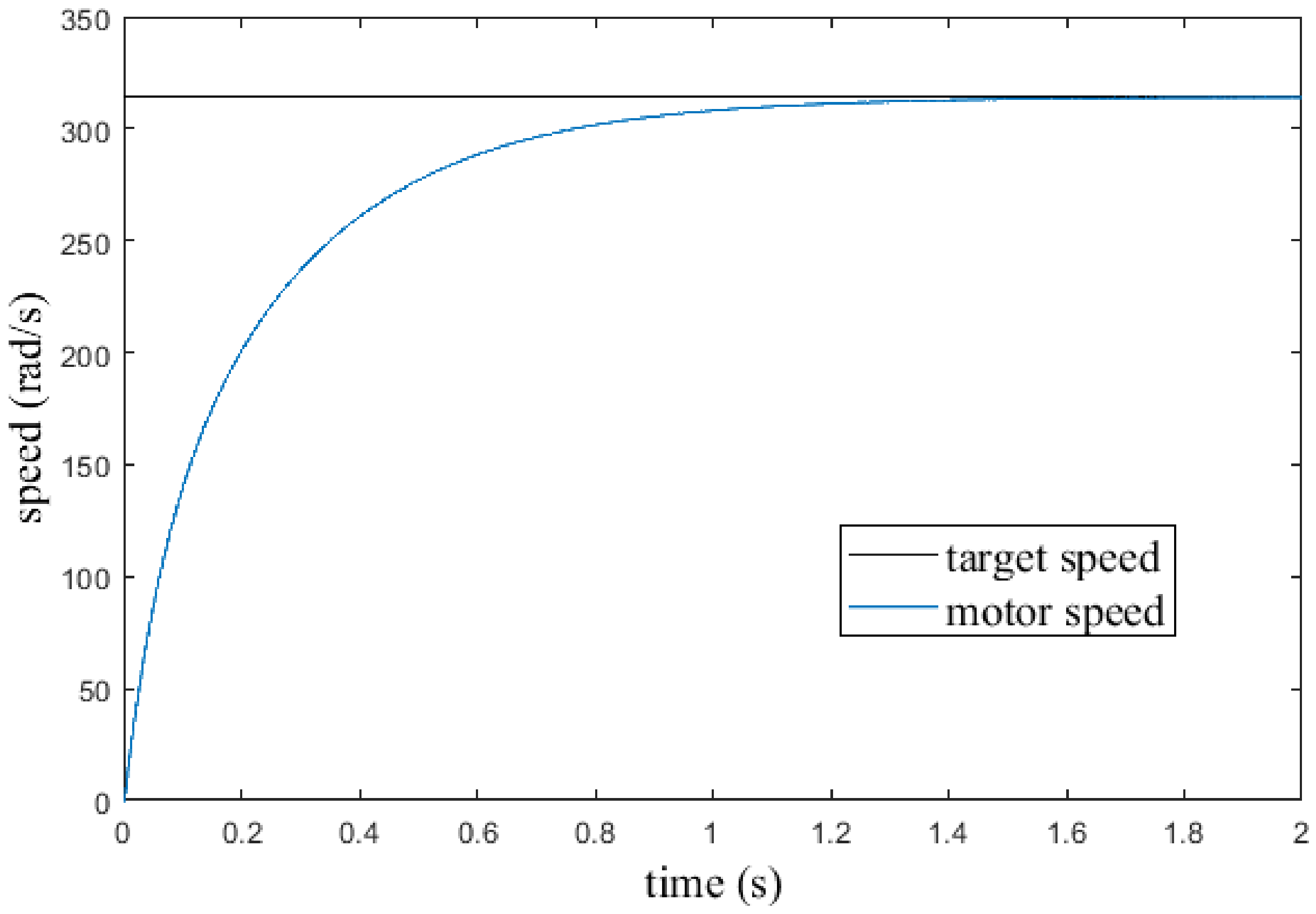
In simulation experiments, the target speed of the motor was set to 50 r/s (revolutions per second), i.e., 50 × 2 π rad/s (radians per second), and the motor speed curve was obtained by starting the motor, as shown in Figure 4.
It can be observed from Figure 4 that the motor speed gradually increased and achieved the set target speed in about 1.5 s before remaining stable. The speed profile indicates that the EKF-based control system had satisfactory performance for speed adjustment of the PMSM.
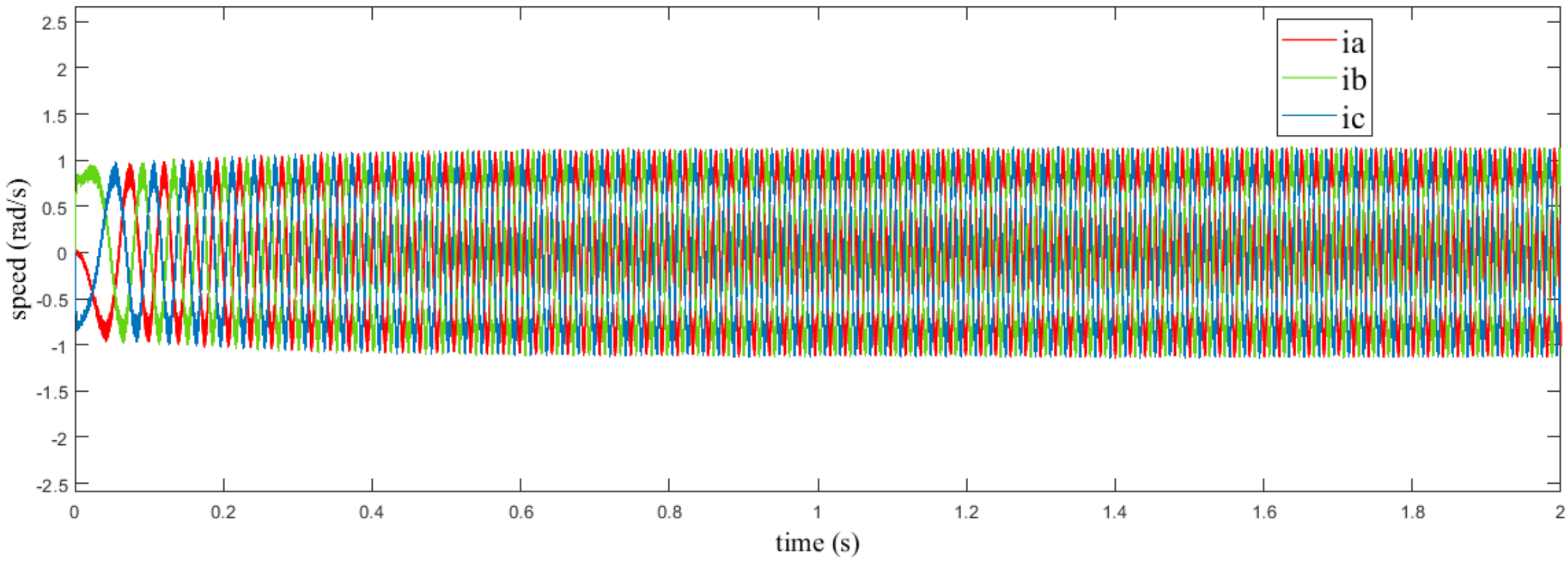
In the simulation experiment, the experiment time was 2 s. Figure 5 shows the variation waveform of the three-phase current waveform of the PMSM.
As shown in Figure 5, ia, ib, and ic were the three-phase current waveforms generated by the motor in operation, and it can be seen that the currents in each phase showed a sinusoidal form of change, and the amplitudes of the three-phase currents were kept balanced in the process, which maintained the normal operation of the motor.
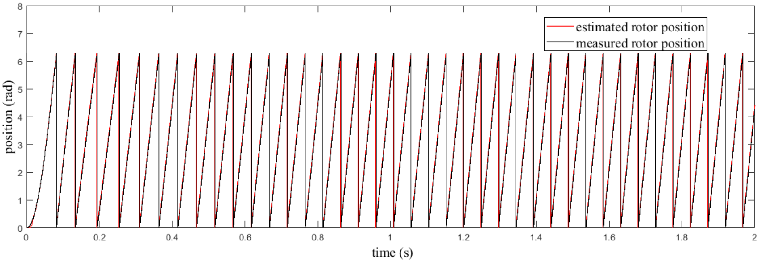
In the simulation experiments, to verify the correctness of the rotor position output from the EKF, the rotor position information output from the EKF was contrasted with the rotor position information obtained from the measurements in Figure 6.
As shown in Figure 6, the rotor position estimated by the extended Kalman filter almost coincides with the rotor position information obtained from measurement, which demonstrates that the extended Kalman filter has a positive influence on the estimation of the rotor position of the motor, that the estimated position is consistent with the actual rotor position information, and that this is a reliable method of obtaining the rotor position. Therefore, in this paper, we selected the extended Kalman filter, and we continued to carry out experiments on the hardware platform.

4.2. Hardware Platform

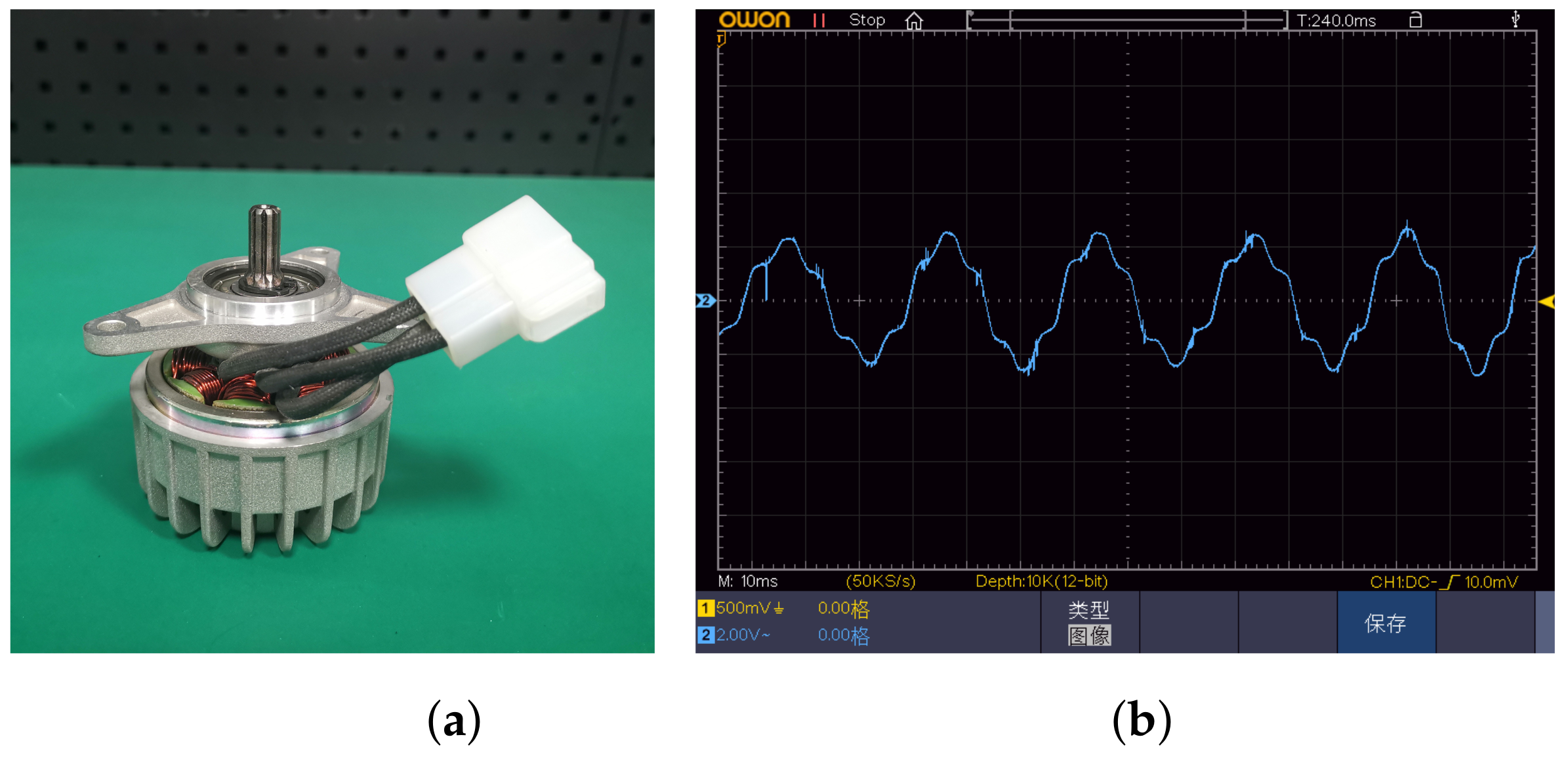
Based on the performance requirements for the actual work of the lawnmower, we selected a PMSM suitable for the lawnmower. Table 2 shows the parameter information of this PMSM, and Figure 7 displays a picture of this PMSM as well as its back electromotive force (BEMF) waveform.
Figure 8 shows the overview of the experimental platform, which includes a controller with STM32F407 as the main control chip, designed by STMicroelectronics and manufactured in Taiwan, China, a three-phase full-bridge driver board, a 500 W PMSM, a motor performance test system, and a PC. The motor performance test system (referred to as a dynamometer) is a machine that specializes in testing the operating performance of motors by applying loads to running motors, and its main testing parameters include motor speed, current, and torque, among others. During the testing process, the dynamometer was capable of real-time data acquisition, and we evaluated the performance of the constructed motor control system by designing different experiments and analyzing the collected data.
Figure 9 shows the logical block diagram of the experimental platform, in which the PWM function of STM32 was used to control the gate driver chip, which, in turn, controlled the three-phase full-bridge drive circuit to realize control of the motor. The ADC function was used to collect voltage and current signals, the EKF was used to estimate the speed of the motor and the rotor position information, and the STM32 communicated with the PC through the USART, which was used for debugging of the program and the acquisition of the data from the serial port of the host computer. The PMSM was connected to the information acquisition end of the dynamometer through coupling in order to realize the function of data acquisition as well as to apply load to the motor.

4.3. Parameter Selection

4.3.1. Parameters of the Current Loop PI Controller

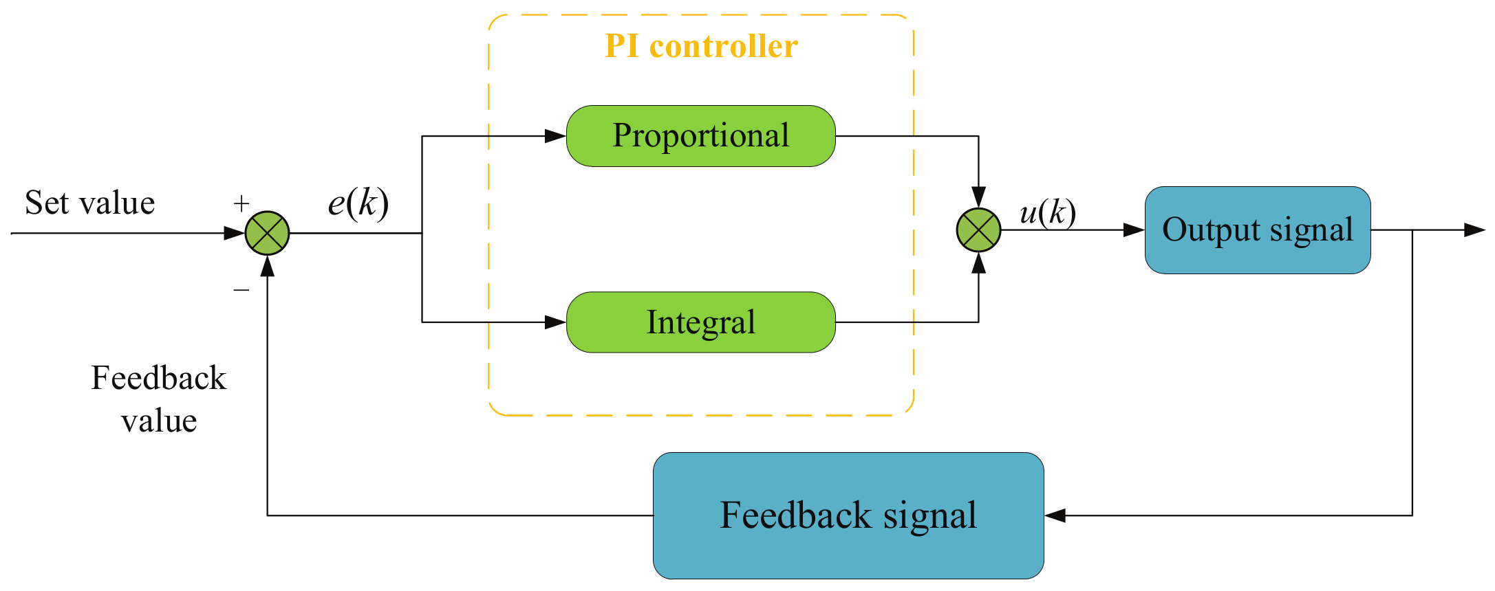
The block diagram of the PI control system used in the experiment is shown in Figure 10.
The output u ( k ) of the PI controller is as follows:
u ( k ) = K p e ( k ) + K I i = 0 e ( i )
where e ( k ) represents the error. Since the controller samples the current at a very high rate, which was set to 10 KHz in this experiment, no differentiation term is introduced. The PI current controller parameters were set in this paper according to the following rules.
The K p and K i parameters for the d-axis were calculated as follows:
K p _ d = α L d
K I _ d = α R
The K p and K i parameters for the q-axis were calculated as follows:
K p _ q = α L q
K I _ q = α R
where L d is the inductance of the d-axis, and L q is the inductance of the q-axis. The value of α is as follows:
α = 2 π / τ , τ = m i n L d / R , L q / R
where τ is the motor time constant. Since L d = L q for a surface-mounted PMSM, the PI parameters of the d- and q-axes were equal, i.e., the parameters of the current loop’s d- and q-axes for the PI controllers were obtained as follows:
K p _ c u r r e n t = 2 π R
K i _ c u r r e n t = 2 π R 2 / L
In practice, due to the existence of systematic errors, the above formula needs to be obtained on the basis of K p and K i values in the actual debugging of the control system before using the trial-and-error method according to the actual control effect to determine the final appropriate value.

4.3.2. Parameters of the Speed Loop PI Controller

In the experiment, the PI parameters of the speed loop were calculated using the following equation:
K p _ s p e e d = 2 β J / 3 P ψ
K I _ s p e e d = β K p _ s p e e d
where β is the bandwidth of the velocity loop, which was taken as 50 rad/s in the experiment; J is the rotational inertia of the motor; P is the number of pole pairs of the PMSM; and ψ is the magnetic chain of the motor. In the same way as for current loop debugging, due to the actual existence of error in the experiment, it is necessary to adjust the value of the parameters according to the actual situation through the trial-and-error method to make the control system achieve good results.

4.3.3. Parameters of the Covariance Matrix

Since the statistical properties of the system’s random disturbances and measurement noise were difficult to determine, this led to the selection of the covariance matrix becoming particularly important; only by selecting the appropriate values can the algorithm be guaranteed to converge efficiently and with a certain degree of accuracy. In the mathematical model analysis, the covariance matrices P 0 , Q, and R gave a statistical description of the model error; matrix P 0 contains information about the variance under the initial conditions and mainly affects the convergence speed of the extended Kalman filter under the transient conditions, matrix Q denotes the statistical description of the model, and matrix R denotes the magnitude of the measurement noise.
Since these parameters are usually unknown, in most cases, the parameters P 0 , Q, and R were selected by the trial-and-error method, which is used to make adjustments by constantly changing the values of the parameters and, at the same time, by observing the estimated values of the rotational speed and the rotor position. When the estimated values have the best convergence effect, then the values of P 0 , Q, and R are optimal values. We finally obtained the values of parameters P 0 , Q, and R for the motor control system in this paper by the trial-and-error method as follows:
P 0 = 1 0 0 0 0 1 0 0 0 0 1 0 0 0 0 1 , Q = 0.1 0 0 0 0 0.1 0 0 0 0 0.2 0 0 0 0 0.001 , R = 0.2 0 0 0.2

4.4. No-Load Operation

The speed of the average lawnmower on the market is generally in the range of 4000 to 6000 (revolutions per minute, r/min); therefore, in this paper, the motor speed was set to 4000 r/min, 5000 r/min, and 6000 r/min for the experiments.
There are usually three major indicators to evaluate the performance of a control system: whether the control is accurate, whether the dynamic response is fast enough, and whether the system is stable. Based on the above indicators, the following experimental program for the performance evaluation of the motor control system was developed:
1.
No-load operation;
2.
Acceleration and deceleration operation;
3.
Different load operation;
4.
Simulation of the typical working conditions of the lawnmower.
For a comprehensive evaluation of the motor control system, the most basic and most critical test was the no-load running of the motor. This involved starting and running the motor without any external load in order to test its ability to start successfully and remain stable after reaching the target speed. This test was used to assess the feasibility and stability of the control system and to accumulate effective experience for subsequent load experiments.
This experiment allowed for the examination of changes to the motor speed, current, and rotor position information. The control system’s ability to regulate the motor speed was evaluated by detecting the rotational speed change in the motor after starting in a no-load condition. Additionally, the motor current was detected and recorded in order to provide data support for subsequent speed regulation and load experiments. The rotor position information was also recorded in order to provide a reference for adjusting the control system.
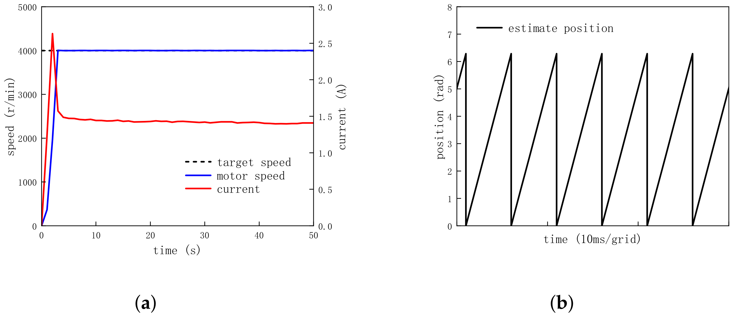
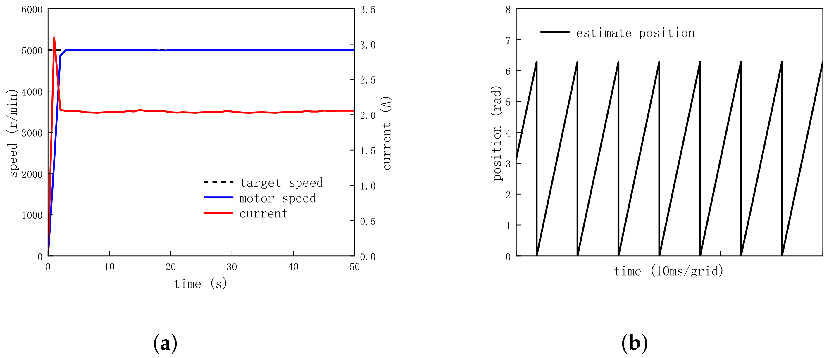
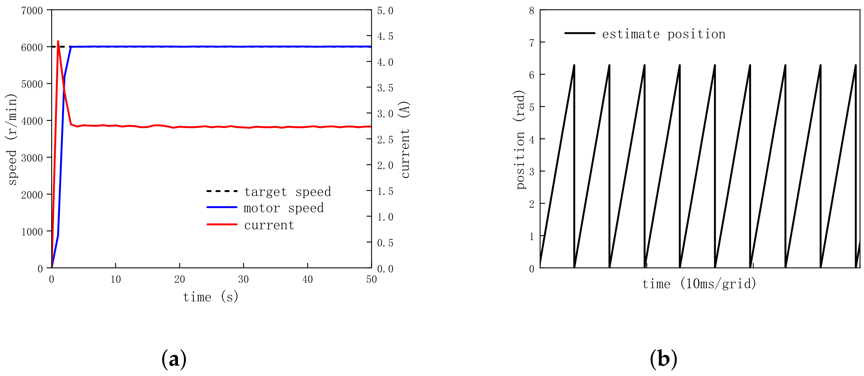
During the experiment, the motor’s target speed was set to run at 4000 r/min, 5000 r/min, and 6000 r/min for a specified period. The dynamometer was used to detect the motor’s speed and current information, while the PC was used to obtain the rotor position information of the motor output from the extended Kalman filter. Figure 11a, Figure 12a and Figure 13a record the variations in motor speed and current; Figure 11b, Figure 12b and Figure 13b record the rotor position information output by the EKF.
In subfigure (a) of Figure 11, Figure 12 and Figure 13, the motor speed reached the target speed in about 3 s and remained stable during the subsequent operation, and the motor current increased rapidly at the beginning of the startup before decreasing rapidly and then remaining stable. The motor speed stabilized at the target speed rapidly after starting, which proves that the control system has an excellent starting ability and can effectively realize the control and regulation of the motor speed. The impact phenomenon of the current is called the starting current and is due to the mechanical resistance at the beginning of the starting process and the inductance inside the motor; after the starting current, it can be seen that the current curve was kept stable. This proves that the control system had good current regulation ability and that it could realize the regulation and the control of the speed by adjusting the current. Table 3 records the peak current at startup, and Figure 11, Figure 12 and Figure 13 show the current during stable motor operation of the PMSM, which provides practical reference data for subsequent speed regulation and load experiments.
In subfigure (b) of Figure 11, Figure 12 and Figure 13, the rotor position information output from the extended Kalman filter changed smoothly under different motor speeds, and the value’s range was basically between 0–2 π . It can also be seen that the higher the speed, the higher the frequency of change of the rotor position information, and that the frequency was in line with the theoretical value, which proves that the EKF provides stable and reliable rotor position information in the control system and thus provides a reliable guarantee for the closed-loop control of the motor speed.

4.5. Acceleration and Deceleration Operation

In the actual work of the lawnmower, the operator can carry out the mowing operation by adjusting to different motor speeds. In order to test the speed control ability of the motor control system and to evaluate the system’s responsiveness and stabilization ability under different speeds and speed change directions, two kinds of speed control operation experiments, namely an acceleration operation and a deceleration operation, were carried out as follows:
1.
Set the target speed from 4000 r/min to 5000 r/min and then to 6000 r/min for the acceleration operation;
2.
Set the target speed from 6000 r/min to 5000 r/min and then to 4000 r/min for the deceleration operation.
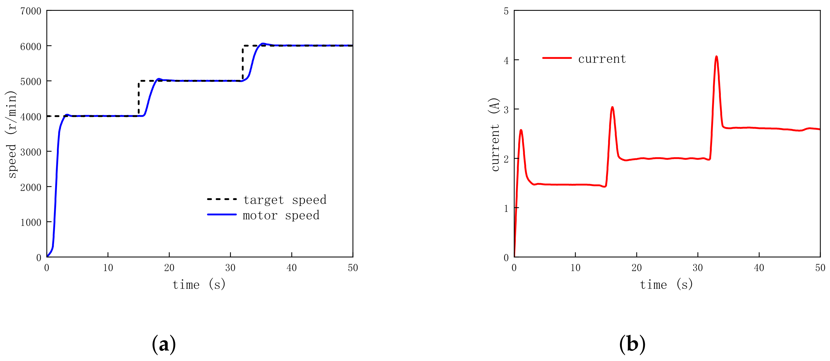
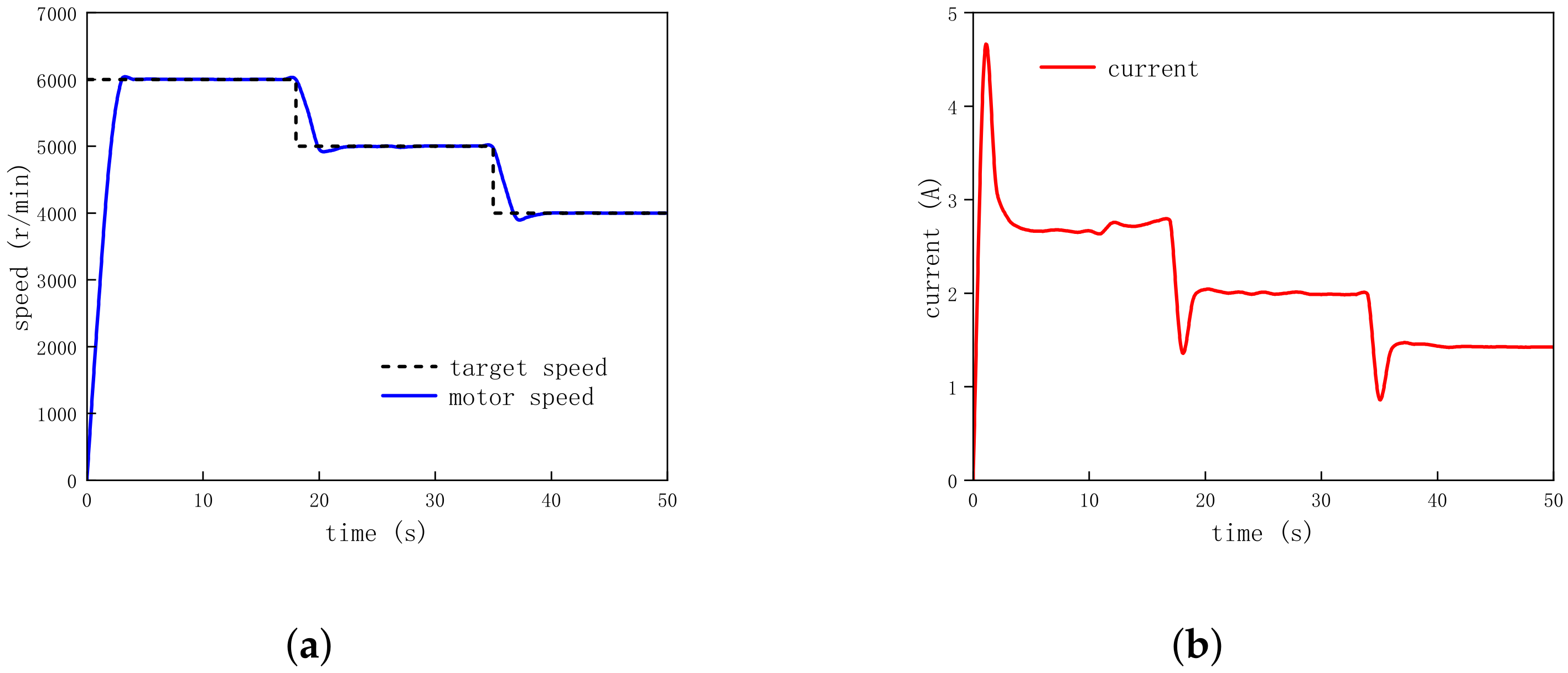
In the experiment, the target speed was continuously changed to test the motor control system’s ability to regulate the speed. Figure 14 records the motor speed change as well as the current change during the acceleration operation. Figure 15 records the motor speed change as well as the current change during the deceleration operation.
In Figure 14a, after the motor was started at the target speed of 4000 r/min, the motor speed change was consistent with the effect of the no-load operation experiment; when the target speed increased to 5000 r/min, the motor speed also increased to 5000 r/min, and when the target speed increased to 6000 r/min, the motor speed also increased to 6000 r/min. It can be seen that in the acceleration operation, the motor speed response was immediate, the overshoot after reaching the target speed was small, and the subsequent operation remained stable. In Figure 14b, as the target speed increased, the current gradually increased, which was a dynamic adjustment made by the motor control system to control the motor speed; the current was adjusted in order to reach the target speed.
In Figure 15a, after the motor was started at the target speed of 6000 r/min, the speed change was consistent with the effect in the no-load running experiment; when the target speed was reduced to 5000 r/min, the motor speed was also reduced to 5000 r/min, and when the target speed was reduced to 4000 r/min, the motor speed was also reduced to 4000 r/min. It can be observed that the motor speed response was also immediate in the deceleration speed operation, and the system controlled the speed accurately. In Figure 15b, the change in current was opposite to that of the acceleration operation, which is also due to the dynamic adjustment made by the motor control system; the output current was adjusted to control the motor speed and to reach the target speed.
Through the above experiments involving motor speed acceleration and deceleration operations, it was proven that the control system is able to effectively adjust the current output to match the set target speed through the process of speed regulation, that the motor speed fluctuation was small during the process of regulation, and that the motor was able to stabilize to the target value rapidly, which proves that the control system has a flexible control capacity regarding the motor speed.

4.6. Different Load Operations

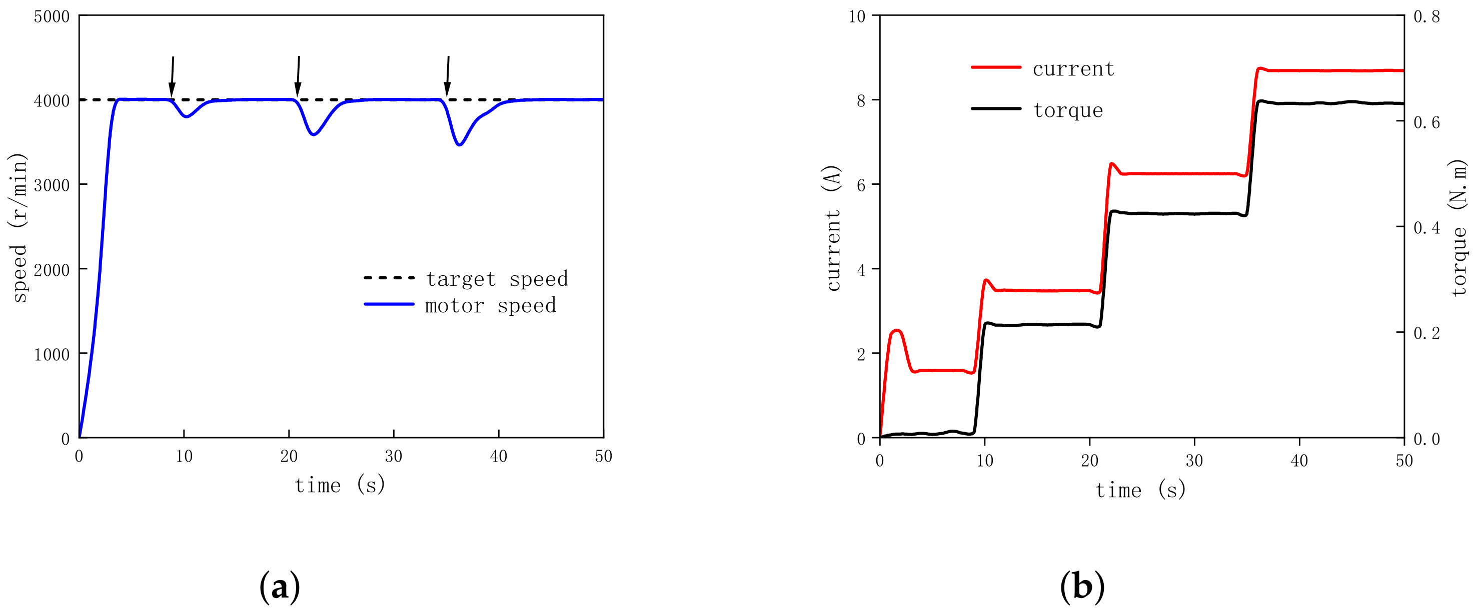
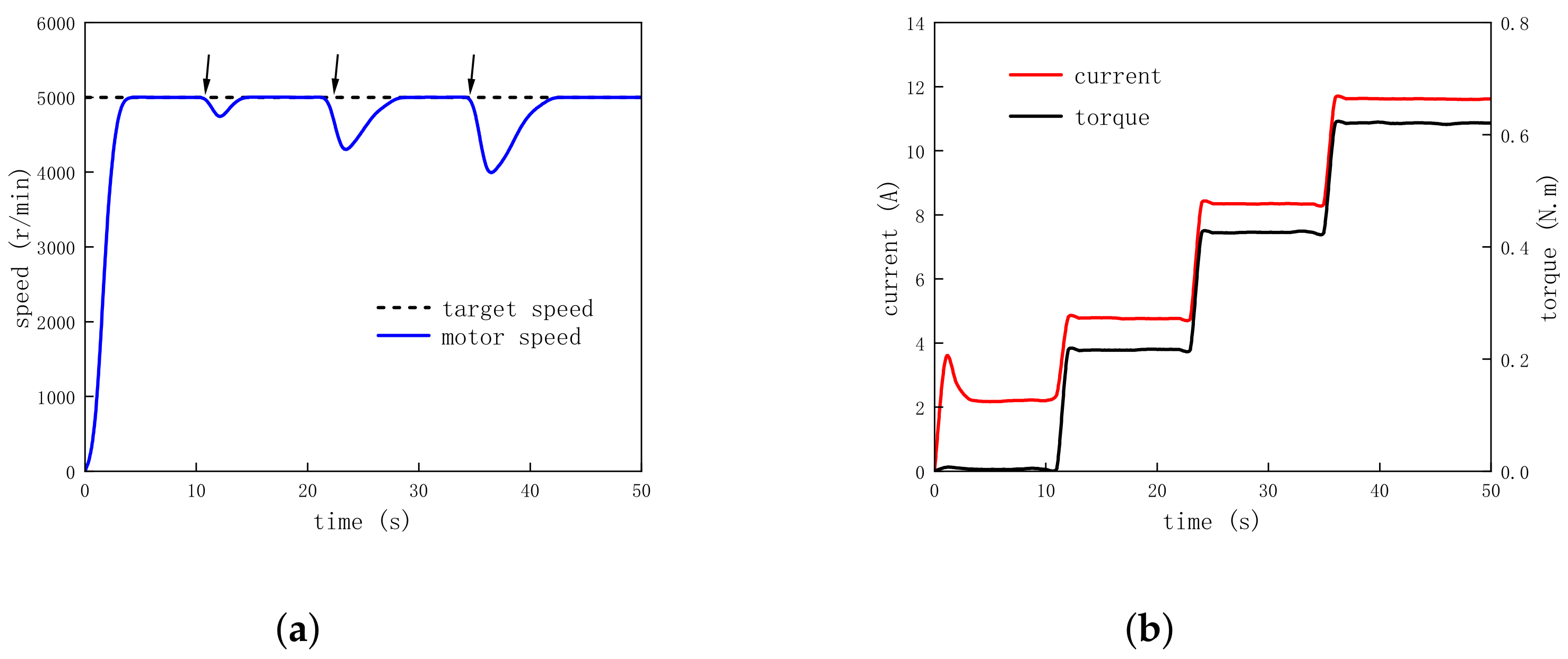
A lawnmower will encounter different sizes of loads during actual operation. To test the performance of the motor control system under different load values, this experiment applied different values of torque to the running motor to simulate the lawnmower encountering different loads in operation and to test the load resistance of the control system. Since the rated torque of the PMSM selected for this paper was 0.6 N·m, loads of 0.2 N·m, 0.4 N·m, and 0.6 N·m were selected for the experiment in order to test the operating effect of the motor under loads at 4000 r/min, 5000 r/min, and 6000 r/min.
In Figure 16, Figure 17 and Figure 18, subfigure (a) records the speed variation curves of the motor running at different target speeds and subjected to different loads, and the three black arrows in the figure represent the three moments when the loads were applied, wherein the first load applied was 0.2 N·m, the second load applied was 0.4 N·m, and the third load applied was 0.6 N·m. Subfigure (b) in the aforementioned figures records the variation in motor current and torque under the above experimental conditions.
In subfigure (a) of Figure 16, Figure 17 and Figure 18, the speed of the motor decreased three times when it was loaded, and the bigger the load, the more obvious the decrease in the speed was. However, the speed of the motor rose immediately after the decrease and returned to the target speed, which proves that the control system was able to automatically regulate and maintain stability in the face of different load conditions.
In subfigure (b) of Figure 16, Figure 17 and Figure 18, the current rose sharply and the motor torque also rose sharply three times when the motor was loaded, which was due to the fact that the motor needed more current to keep running under the load, so the control system made dynamic adjustments by increasing the current in order to generate more torque to fight against the load and to keep the rotational speed stable.
The above results show that the motor control system was able to make effective dynamic adjustments when encountering different loads and correctly handled the situations concerning load changes so that the motor followed the set target speed, which proves the stability and reliability of the system and shows good dynamic response and strong regulation ability against load disturbances.

4.7. Simulation of the Typical Working Conditions of a Lawnmower

In order to ensure the motor control system can be applied to lawnmower products, in addition to the above tests of no-load, acceleration, deceleration, and different load operations, it was also necessary to carry out experiments simulating the typical working conditions of a lawnmower. Considering that the size of the load force on the lawnmower is constantly changing during the actual mowing operation, in order to simulate the randomness of the size of the load force and to test the performance of the motor control system under typical working conditions, this experiment applied loads with changing values and durations to the running motor. Based on the typical working conditions of the lawnmower, this experiment was divided into two cases:
1.
Lawnmower work in areas of uniform lawn density with smooth load variations;
2.
Lawnmower work in areas of mixed lawn density with random load variations.

4.7.1. Smooth Load Variation Operation

When the lawnmower is working in an area with uniform lawn density, the load size varies smoothly. In order to simulate this condition, the dynamometer was used to set up load variations consistent with this condition.
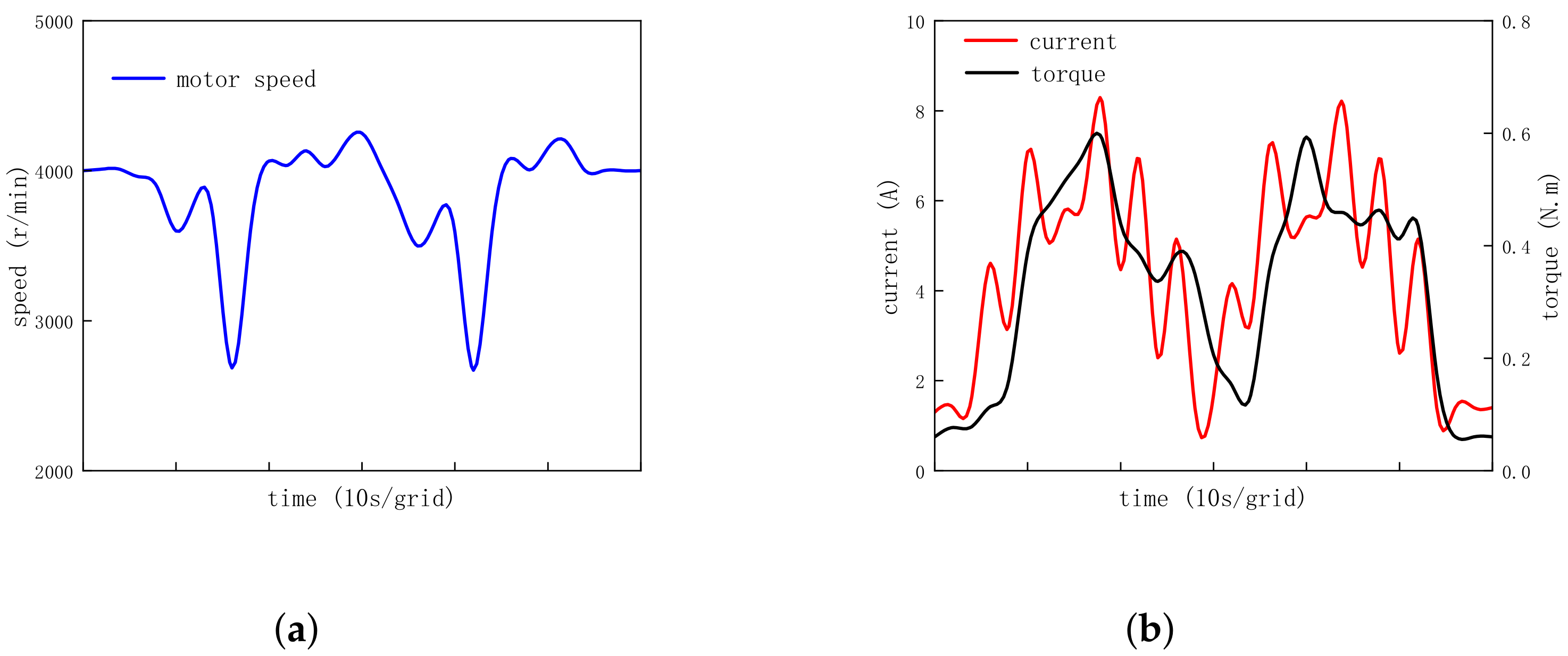
As shown in Table 4, the load value was set to gradually increase from 0.1 N·m to 0.6 N·m and then to gradually decrease to 0.1 N·m. The duration of each load was 2 s, and the implementation period of two indicates that the above process was executed twice in order to increase the dependability of the experimental data.
The target speed of the motor was set to run at 4000 r/min, 5000 r/min, and 6000 r/min, and the loads listed above were applied to the motor running at the three speeds. The motor speeds for this case are recorded in subfigure (a) of Figure 19, Figure 20 and Figure 21, and the motor currents and torques for this case are recorded in subfigure (b) of Figure 19, Figure 20 and Figure 21.
In Figure 19, Figure 20 and Figure 21, the first 30 s and the last 30 s can be regarded as one execution cycle, and it can be observed that the curves for the rotational speed, current, and torque were similar during the two execution cycles. In subfigure (a), it can be seen that due to the continuous change in the load, the motor speed was somewhat reduced and overshot the target speed, but it stabilized at the set target speed eventually. In subfigure (b), it can be seen that the current first rose as the load increased and then fell as the load decreased, and that the torque also demonstrated a tendency to rise and then fall as the current fluctuated.

4.7.2. Random Load Variation Operation

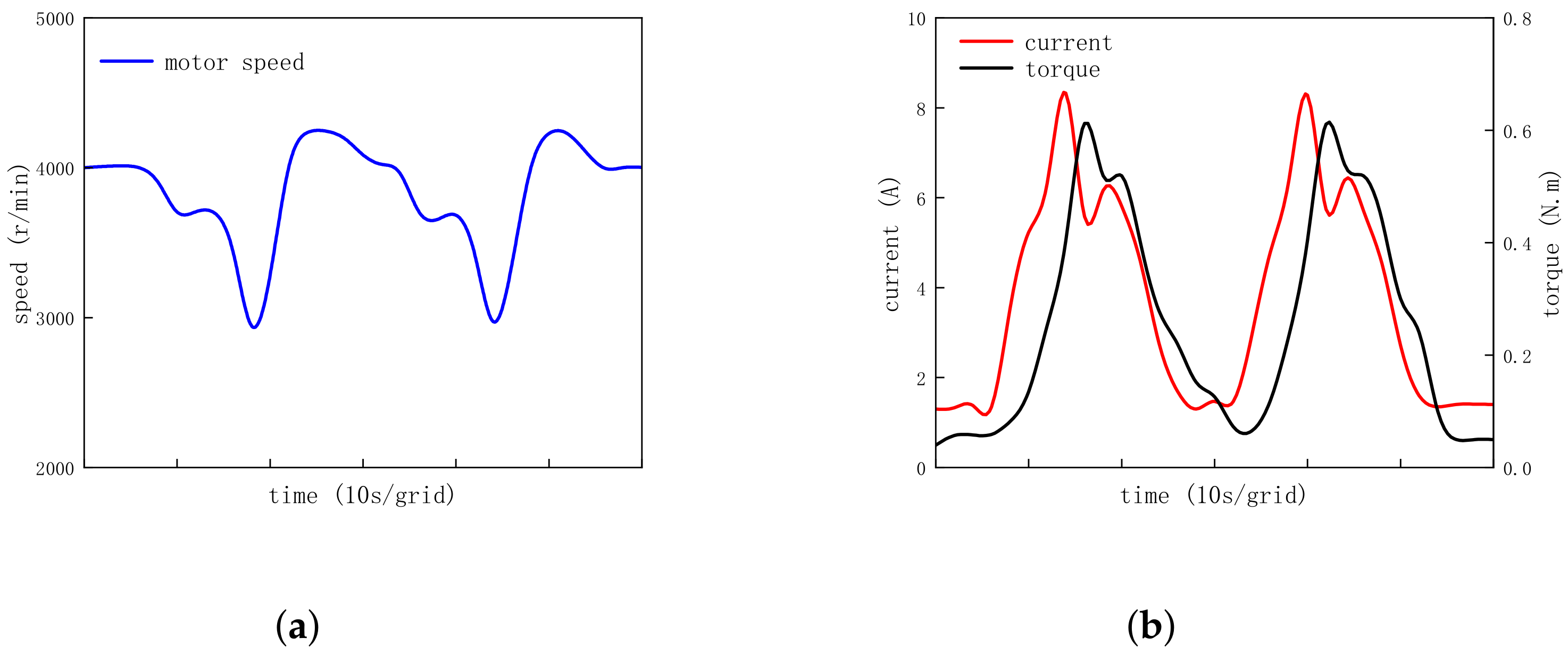
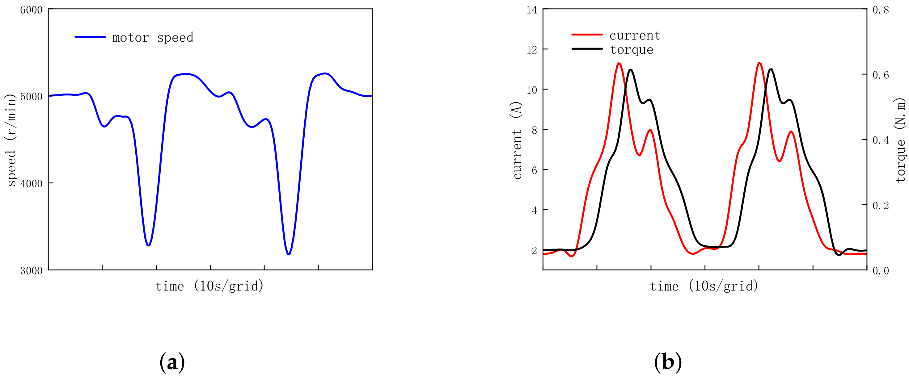
Lawnmowers also operate in areas with mixed lawn densities and with random load sizes without any regularity in size; to simulate this in an experimental setting, the dynamometer was set up with the load changes shown in Table 5.
The size of the loads varied randomly in order to simulate a scenario wherein the lawnmower is working with a cluttered lawn density by setting up cluttered load variations for which, again, the duration of each load was 2 s and the execution period was two.
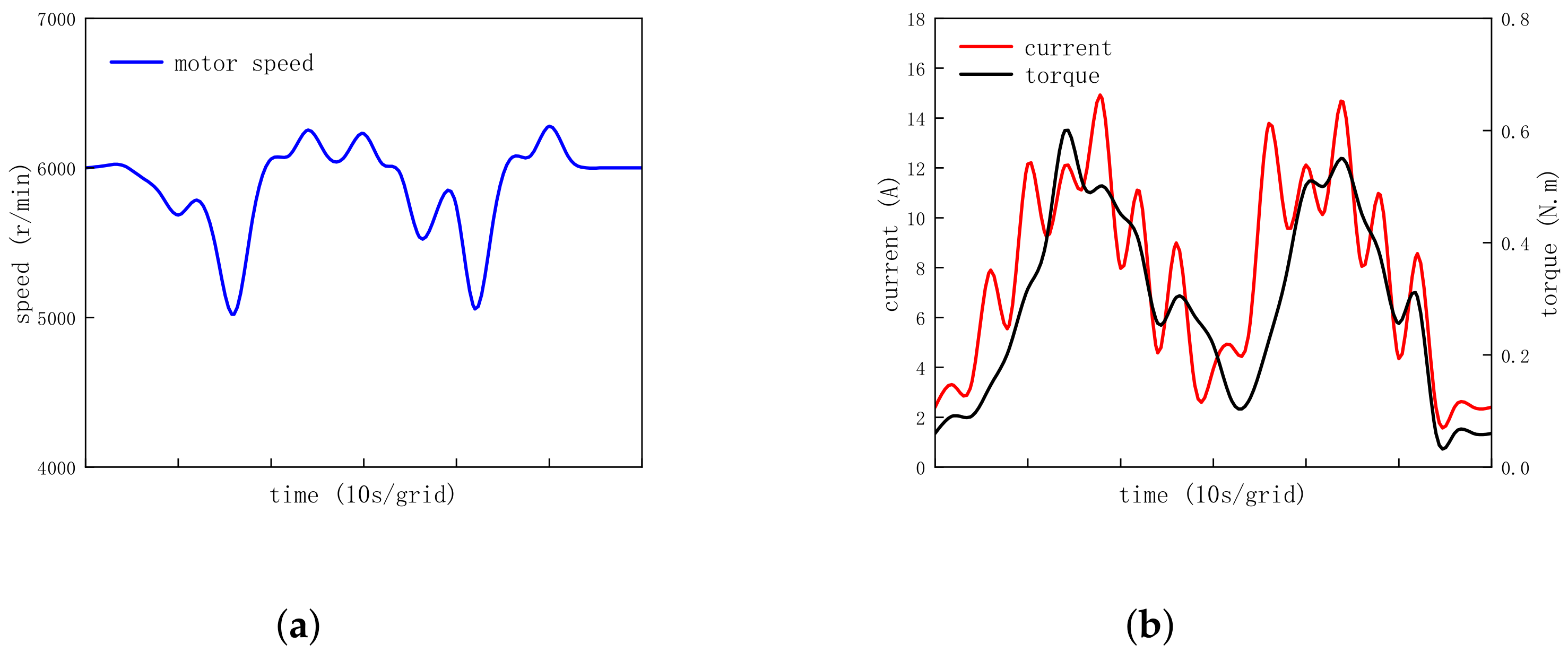
The target speed of the motor was set to run at 4000 r/min, 5000 r/min, and 6000 r/min, and the loads listed above were applied to the motor running at the three speeds. The motor speeds for this case are recorded in subfigure (a) of Figure 22, Figure 23 and Figure 24, and the motor currents and torques for this case are recorded in subfigure (b) of Figure 22, Figure 23 and Figure 24.
In Figure 22, Figure 23 and Figure 24, the first and last 30 s were also regarded as one execution cycle. The rotational speed curve in subfigure (a) fluctuated greatly with the random increases and decreases in the load, but the overall trend stabilized at the target rotational speed. Jittering of the current is obvious in subfigure (b); this was due to the messy and random changes in the load, which caused the control system to dynamically adjust the current in order to cope with the random changes in the load. The degree of torque jitter was slightly weaker than that of the current, which proves that the control system can adjust the torque smoothly to ensure the steady operation of the motor.
In the above two experiments, simulating the typical operating conditions of a lawnmower, the motor control system was able to adapt quickly to the loads in different situations and realize control of the torque by dynamically adjusting the current output, thus controlling the motor speed to stabilize at the target speed. The experiments proved that the motor control system has a good control effect under the typical working conditions of a lawnmower and has excellent dynamic adjustment ability and robustness, and the whole system shows good recovery and controllability.

4.8. Motor Efficiency Monitoring

To assess the performance of the engine system more comprehensively, this paper continues with a motor efficiency test, with the aim of gaining insight into the efficiency changes in the motor under different load conditions and to provide strong data support for subsequent optimization of the system. The torque–efficiency plot of the motor clearly presents the efficiency characteristics of the motor system and reveals its performance at various torque levels.
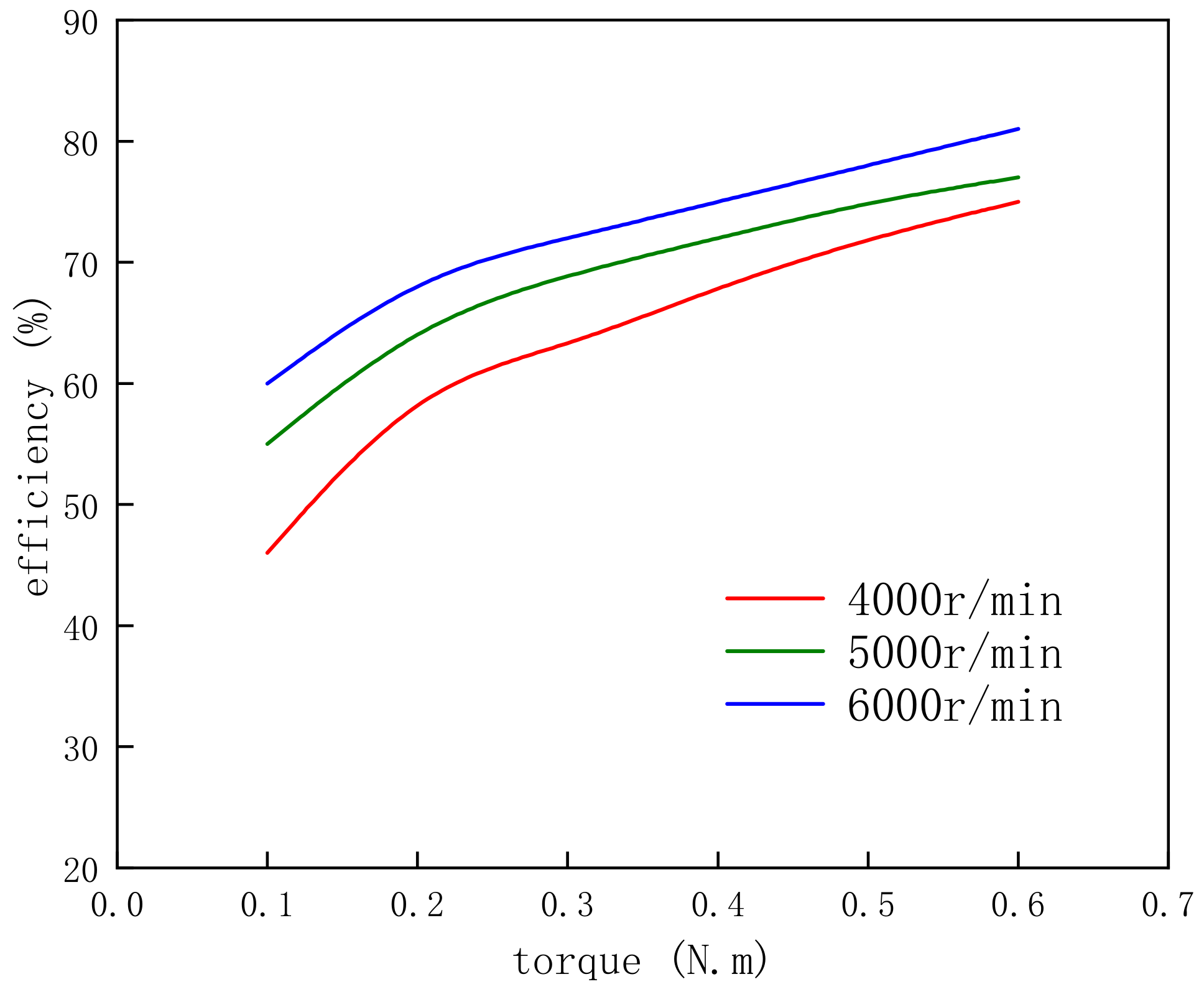
The relationship between motor torque and motor efficiency was recorded for three motor speed scenarios: namely, 4000 r/min, 5000 r/min, and 6000 r/min, as shown in Figure 25.
In Figure 25, the efficiency of the motor shows a steady increase with a gradual increase in torque at each speed. This indicates that the motor system was able to convert the input electrical energy into mechanical energy more efficiently under different load conditions and to achieve higher efficiencies under different loads.
Comparing the curves at different speeds, it can be observed that the motor system achieved higher efficiency at the same torque level at higher speeds. This reflects the fact that the motor can cope with certain load requirements more efficiently when operating at high speeds as opposed to low speeds. This provides an important guide for motor performance tuning and selection for lawnmower application scenarios and provides a strong basis for future control system optimization and improvement.

5. Conclusions

In this paper, a permanent magnet synchronous motor sensorless vector control system for a lawnmower was designed and implemented. A PMSM, with a power of 500 W was selected as the research object, and an extended Kalman filter was adopted as the method of sensorless control. The reliability and performance of the system were verified through a series of experiments.
Firstly, no-load operation experiments were conducted and aimed to evaluate the stability of the system under light load conditions. Secondly, acceleration and deceleration operation experiments were conducted in order to verify the system’s responsiveness and control effectiveness under dynamic adjustment. In the different load operation experiments, the stability and performance of the system during operation were further examined. In order to simulate scenarios of the lawnmower during realistic operation, uniformly varying load and randomly varying load experiments were carried out; these examined the robustness and adaptability of the system under different load variation modes.
The experimental results showed that the control system has significant practicality and stability for its application in lawnmowers, shows good performance under various working conditions, successfully realizes the efficient control of a permanent magnet synchronous motor, and provides practical design experience as well as data-based evidence for the field of lawnmower motor control.
In future works, research can be carried out in a real turf environment, taking into account the influence of factors such as terrain, humidity, turf type, etc., in order to provide more reliable data to support the practical application of the system and to provide a greater guarantee of practicality and reliability for its promotion and development in practical applications.

Author Contributions

Conceptualization, D.S., D.W. and D.H.; methodology, D.S. and D.W.; software, D.S. and D.H.; validation, D.S., D.W. and D.H.; formal analysis, D.W. and D.H.; investigation, D.S. and D.W.; resources, D.S.; data curation, D.W.; writing—original draft preparation, D.S.; writing—review and editing, D.H. and P.Z.; visualization, D.W.; supervision, D.S., D.H. and P.Z.; project administration, D.S.; funding acquisition, D.S. All authors have read and agreed to the published version of the manuscript.

Funding

This research was funded by the Key R&D Plan of Shandong Province (Major Science and Technology Innovation Project), grant number 2023CXGC010701; and the Project of Shandong Provincial Major Scientific and Technological Innovation, grant number 2019TSLH0315.

Data Availability Statement

Data available on request due to privacy. The data presented in this study are available on request from the corresponding author.

Conflicts of Interest

The authors declare no conflicts of interest.

References

  1. Kang, C.Q.; Ng, P.K.; Liew, K.W. The Conceptual Synthesis and Development of a Multifunctional Lawnmower. Inventions 2021, 6, 38. [Google Scholar] [CrossRef]
  2. Ibrahim, B.; Brahmaiah, V.S.; Sharma, P. Design of smart autonomous remote monitored solar powered lawnmower robot. Mater. Today Proc. 2020, 28, 2338–2344. [Google Scholar] [CrossRef]
  3. Saji, A.; Bastian, G.G.; Muhammad Jaseel, K.; Sajeevan, S. Design and Implementation of Intelligent Lawn-Mower Robot. Int. J. Innov. Sci. Res. Technol. 2018, 3, 477–480. [Google Scholar]
  4. Daniyan, I.; Balogun, V.; Adeodu, A.; Oladapo, B.; Peter, J.K.; Mpofu, K. Development and performance evaluation of a robot for lawn mowing. Procedia Manuf. 2020, 49, 42–48. [Google Scholar] [CrossRef]
  5. Dutta, P.P.; Baruah, A.; Konwar, A. A technical review of lawn mower technology. ADBU J. Eng. Technol. 2016, 4, 179–182. [Google Scholar]
  6. Tahir, T.; Khalid, A.; Arshad, J.; Haider, A.; Rasheed, I.; Rehman, A.U.; Hussen, S. Implementation of an IoT-Based Solar-Powered Smart Lawn Mower. Wirel. Commun. Mob. Comput. 2022, 2022, 1–12. [Google Scholar] [CrossRef]
  7. Wirtz, J.; Patterson, P.G.; Kunz, W.H.; Gruber, T.; Lu, V.N.; Paluch, S.; Martins, A. Brave new world: Service robots in the frontline. J. Serv. Manag. 2018, 29, 907–931. [Google Scholar] [CrossRef]
  8. Ahn, H.; Park, H.; Kim, C.; Lee, H. A Review of State-of-the-art Techniques for PMSM Parameter Identifi-cation. J. Electr. Eng. Technol. 2020, 15, 1177–1187. [Google Scholar] [CrossRef]
  9. Wang, Q.; Wang, S.; Chen, C. Review of sensorless control techniques for PMSM drives. IEEJ Trans. Electr. Electron. Eng. 2019, 14, 1543–1552. [Google Scholar] [CrossRef]
  10. Türker, T.; Buyukkeles, U.; Bakan, A.F. A robust predictive current controller for PMSM drives. IEEE Trans. Ind. Electron. 2016, 63, 3906–3914. [Google Scholar] [CrossRef]
  11. Linares-Flores, J.; Garcia-Rodriguez, C.; Sira-Ramirez, H.; Ramirez-Cardenas, O.D. Robust backstepping tracking controller for low-speed PMSM positioning system: Design, analysis, and implementation. IEEE Trans. Ind. Inform. 2015, 11, 1130–1141. [Google Scholar] [CrossRef]
  12. Bida, V.M.; Samokhvalov, D.V.; Al-Mahturi, F.S. PMSM vector control techniques—A survey. In Proceedings of the 2018 IEEE Conference of Russian Young Researchers in Electrical and Electronic Engineering (EIConRus), Moscow and St. Petersburg, Russia, 29 January–1 February 2018; pp. 577–581. [Google Scholar]
  13. Wang, T.; Huang, J.; Ye, M.; Chen, J.; Kong, W.; Kang, M.; Yu, M. An EMF observer for PMSM sensorless drives adaptive to stator re-sistance and rotor flux linkage. IEEE J. Emerg. Sel. Top. Power Electron. 2018, 7, 1899–1913. [Google Scholar] [CrossRef]
  14. Bao, D.; Pan, X.; Wang, Y.; Wang, X.; Li, K. Adaptive synchronous-frequency tracking-mode observer for the sensor-less control of a surface PMSM. IEEE Trans. Ind. Appl. 2018, 54, 6460–6471. [Google Scholar] [CrossRef]
  15. Yan, H.; Wang, W.; Xu, Y.; Zou, J. Position sensorless control for PMSM drives with single current sensor. IEEE Trans. Ind. Electron. 2022, 70, 178–188. [Google Scholar] [CrossRef]
  16. Novak, Z.; Novak, M. Adaptive PLL-based sensorless control for improved dynamics of high-speed PMSM. IEEE Trans. Power Electron. 2022, 37, 10154–10165. [Google Scholar] [CrossRef]
  17. Xuan Mung, N.; Nguyen, N.P.; Pham, D.B.; Dao, N.N.; Hong, S.K. Synthesized landing strategy for quadcopter to land pre-cisely on a vertically moving apron. Mathematics 2022, 10, 1328. [Google Scholar] [CrossRef]
  18. Volpato Filho, C.J.; Xiao, D.; Vieira, R.P.; Emadi, A. Observers for high-speed sensorless pmsm drives: Design methods, tuning challenges and future trends. IEEE Access 2021, 9, 56397–56415. [Google Scholar] [CrossRef]
  19. Wang, G.; Yang, L.; Zhang, G.; Xu, D. Comparative investigation of pseudorandom high-frequency signal injection schemes for sensorless IPMSM drives. IEEE Trans. Power Electron. 2016, 32, 2123–2132. [Google Scholar] [CrossRef]
  20. Wang, S.; Yang, K.; Chen, K. An improved position-sensorless control method at low speed for PMSM based on high-frequency signal injection into a rotating reference frame. IEEE Access 2019, 7, 86510–86521. [Google Scholar] [CrossRef]
  21. Chen, D.; Lu, K.; Wang, D. An If Startup method with compensation loops for pmsm with smooth transition. IEEJ J. Ind. Appl. 2020, 9, 263–270. [Google Scholar] [CrossRef]
  22. Nair, S.V.; Hatua, K.; Prasad, N.D.; Reddy, D.K. A Quick I-F Starting of PMSM Drive With Pole Slipping Preven-tion and Reduced Speed Oscillations. IEEE Trans. Ind. Electron. 2020, 68, 6650–6661. [Google Scholar] [CrossRef]
  23. Mesloub, H.; Boumaaraf, R.; Benchouia, M.T.; Goléa, A.; Goléa, N.; Srairi, K. Comparative study of conventional DTC and DTC_SVM based control of PMSM motor—Simulation and experimental results. Math. Comput. Simul. 2020, 167, 296–307. [Google Scholar] [CrossRef]
  24. Song, X.; Fang, J.; Han, B.; Zheng, S. Adaptive compensation method for high-speed surface PMSM sensorless drives of EMF-based position estimation error. IEEE Trans. Power Electron. 2015, 31, 1438–1449. [Google Scholar] [CrossRef]
  25. Mohd Zaihidee, F.; Mekhilef, S.; Mubin, M. Robust speed control of PMSM using sliding mode control (SMC)—A review. Energies 2019, 12, 1669. [Google Scholar] [CrossRef]
  26. Chi, X.; Wang, C.; Wu, Q.; Yang, J.; Lin, W.; Zeng, P.; Li, H.; Shao, M. A ripple suppression of sensorless FOC of PMSM electrical drive system based on MRAS. Results Eng. 2023, 20, 101427. [Google Scholar] [CrossRef]
  27. Li, M.; Lv, K.; Wen, C.; Zhao, Q.; Zhao, X.; Wang, X. Sensorless control of permanent magnet synchronous linear motor based on sliding mode variable structure MRAS flux observation. Prog. Electromagn. Res. Lett. 2021, 101, 89–97. [Google Scholar] [CrossRef]
  28. Yang, H.; Yang, R.; Hu, W.; Huang, Z. FPGA-based sensorless speed control of PMSM using enhanced perfor-mance controller based on the reduced-order EKF. IEEE J. Emerg. Sel. Top. Power Electron. 2019, 9, 289–301. [Google Scholar] [CrossRef]
  29. Gong, C.; Hu, Y.; Gao, J.; Wang, Y.; Yan, L. An improved delay-suppressed sliding-mode observer for sensorless vec-tor-controlled PMSM. IEEE Trans. Ind. Electron. 2019, 67, 5913–5923. [Google Scholar] [CrossRef]
  30. Niedermayr, P.; Alberti, L.; Bolognani, S.; Abl, R. Implementation and experimental validation of ultra-high-speed pmsm sensorless control by means of extended kalman filter. IEEE J. Emerg. Sel. Top. Power Electron. 2020, 10, 3337–3344. [Google Scholar] [CrossRef]
  31. Toso, F.; Da Ru, D.; Alotto, P.; Bolognani, S. A moving horizon estimator for the speed and rotor position of a sensorless PMSM drive. IEEE Trans. Power Electron. 2018, 34, 580–587. [Google Scholar] [CrossRef]
  32. Anwer, A.M.O.; Omar, F.A.; Bakir, H.; Kulaksiz, A.A. Sensorless control of a PMSM drive using EKF for wide speed range supplied by MPPT based solar PV system. Elektron. Ir Elektrotechnika 2020, 26, 32–39. [Google Scholar] [CrossRef]
  33. Do, T.D.; Xuan-Mung, N.; Nguyen, N.P.; Lee, J.W.; Lee, Y.S.; Lee, S.T.; Hong, S.K. Multi-sensor-based Target Pose Estimation for Autonomous Precision Perching of Nano Aerial Vehicles. In Proceedings of the 2022 22nd International Conference on Control, Automation and Systems (ICCAS), Jeju, Republic of Korea, 27 November–1 December 2022; pp. 1565–1571. [Google Scholar]
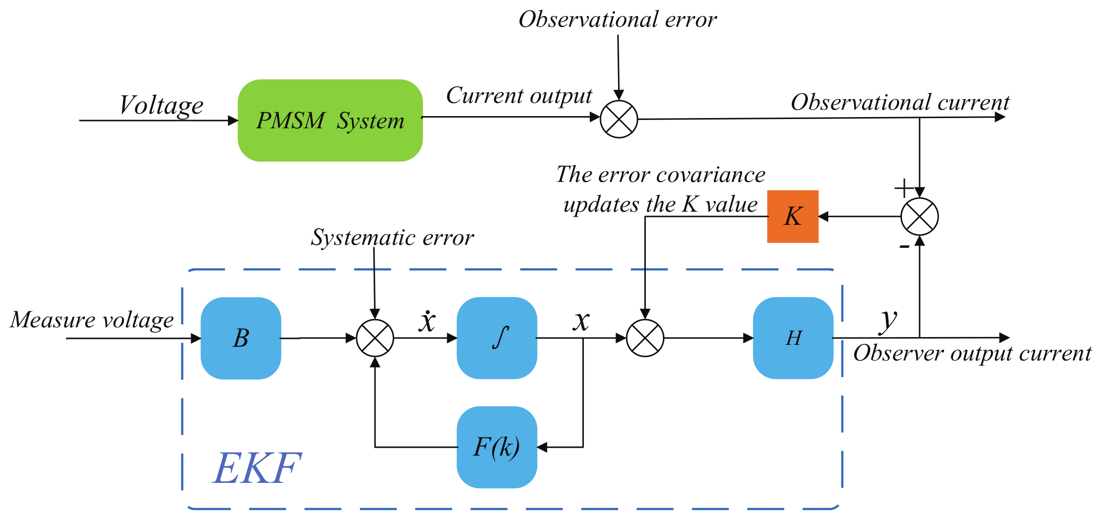
Figure 1. Block diagram of EKF implementation.
Energies 17 01230 g001
Figure 2. The flowchart of the EKF algorithm for a PMSM.
Energies 17 01230 g002
Figure 3. Block diagram of the PMSM sensorless vector control system.
Energies 17 01230 g003
Figure 4. Motor speed in the simulation experiment.
Energies 17 01230 g004
Figure 5. Motor three-phase current in the simulation experiment.
Energies 17 01230 g005
Figure 6. Estimated motor position and measured motor position.
Energies 17 01230 g006
Figure 7. The PMSM used in the experiment. (a) Picture of the PMSM; (b) BEMF waveform of the PMSM.
Energies 17 01230 g007
Figure 8. Overview of the experimental platform.
Energies 17 01230 g008
Figure 9. Logical block diagram of the experimental platform.
Energies 17 01230 g009
Figure 10. Logical block diagram of PI controller.
Energies 17 01230 g010
Figure 11. No-load operation at 4000 r/min. (a) Motor speed and current; (b) rotor position taken from the extended Kalman filter.
Energies 17 01230 g011
Figure 12. No-load operation at 5000 r/min. (a) Motor speed and current; (b) rotor position taken from the extended Kalman filter.
Energies 17 01230 g012
Figure 13. No-load operation at 6000 r/min. (a) Motor speed and current; (b) rotor position taken from the extended Kalman filter.
Energies 17 01230 g013
Figure 14. Acceleration operation. (a) Motor speed; (b) motor current.
Energies 17 01230 g014
Figure 15. Deceleration operation. (a) Motor speed; (b) motor current.
Energies 17 01230 g015
Figure 16. Different load operation at 4000 r/min. (a) Motor speed; (b) motor current and torque.
Energies 17 01230 g016
Figure 17. Different load operation at 5000 r/min. (a) Motor speed; (b) motor current and torque.
Energies 17 01230 g017
Figure 18. Different load operation at 6000 r/min. (a) Motor speed; (b) motor current and torque.
Energies 17 01230 g018
Figure 19. Smooth load variation operation at 4000 r/min. (a) Motor speed; (b) motor current and torque.
Energies 17 01230 g019
Figure 20. Smooth load variation operation at 5000 r/min. (a) Motor speed; (b) motor current and torque.
Energies 17 01230 g020
Figure 21. Smooth load variation operation at 6000 r/min. (a) Motor speed; (b) motor current and torque.
Energies 17 01230 g021
Figure 22. Random load variation operation at 4000 r/min. (a) Motor speed; (b) motor current and torque.
Energies 17 01230 g022
Figure 23. Random load variation operation at 5000 r/min. (a) Motor speed; (b) motor current and torque.
Energies 17 01230 g023
Figure 24. Random load variation operation at 6000 r/min. (a) Motor speed; (b) motor current and torque.
Energies 17 01230 g024
Figure 25. Motor torque and efficiency at different speeds.
Energies 17 01230 g025
Table 1. Main parameters of the simulated PMSM.
ItemValueUnit
DC supply voltage24V
Flux linkage0.024Wb
Stator resistance0.03ohm
Stator inductance0.08mH
Number of pole pairs3/
Table 2. Main parameters of the PMSM.
ItemValueUnit
Rated voltage36V
Rated power500W
Rated torque0.6N·m
Number of pole pairs3/
Torque coefficient0.036Nm/A
Line-to-line resistance0.055ohm
Line-to-line inductance0.16mH
Table 3. Critical current information under no-load operation.
Target Speed (r/min)Peak Current at Startup (A)Current During Stable Operation (A)
40002.631.42
50003.122.05
60004.452.74
Table 4. Settings for load values and load durations with smooth load variations.
Load Value (N·m)Load Duration (s)Implementation Period
0.12
0.22
0.32
0.42
0.52
0.622
0.52
0.42
0.32
0.22
0.12
Table 5. Settings for load values and load durations with random load variations.
Load Value (N·m)Load Duration (s)Implementation Period
0.32
0.12
0.52
0.22
0.62
0.322
0.52
0.22
0.42
0.12
0.32
Disclaimer/Publisher’s Note: The statements, opinions and data contained in all publications are solely those of the individual author(s) and contributor(s) and not of MDPI and/or the editor(s). MDPI and/or the editor(s) disclaim responsibility for any injury to people or property resulting from any ideas, methods, instructions or products referred to in the content.