Development of 1D Model of Constant-Volume Combustor and Numerical Analysis of the Exhaust Nozzle

Abstract

Pressure gain combustion cycles are under the spotlight due to their higher theoretical cycle thermal efficiency compared to conventional machines. Under this prism, a constant-volume combustor (CVC) prototype supplied with a mixture of air and liquid iso–octane was developed. The efforts of the current study were focused on both creating a 1D model of the experimental test rig for the CVC analysis and a 3D numerical simulation of the exhaust system. The goal of the study was to retrieve the total outlet quantities of the combustor, which would otherwise be difficult to assess experimentally, and to investigate the pulsating flow field at the outlet. First, a thorough description of the reduced order model was accompanied with the model’s validation using the available experimental data of the chamber. Then, the resulting outlet stagnation properties of the CVC were imposed as spatially averaged transient boundary conditions to the 3D exhaust flow domain. The unsteady Reynolds–averaged Navier–Stokes equations were solved for a sufficient number of periods, and the assessment of the out-take system in terms of losses and attenuation was conducted. In conclusion, the analysis of the combustor’s outflow will pave the way for an effective future design of the CVC exhaust system.

1. Introduction

Nowadays, many researchers attempt to analyse, identify, and introduce innovative sustainable energy conversion systems. The gas turbine community performs an overall review of conventional cycles, thus seeking higher levels of performance. Pressure Gain Combustion (PGC) has been individuated as the most promising solution to increase efficiency and reduce specific fuel consumption [1] by using low-carbon fuels (e.g., hydrogen). These unconventional machines [2] were introduced for the first time by Holzwarth [3], who invented the constant-volume combustor (CVC) gas turbine. Their principal concept is hidden to the alternative combustion, iso-choric deflagrative [4], or detonative [5,6], with respect to the conventional quasi-isobaric one. The thermodynamic process of detonation is described with the help of the ZND (Zeldovich, von Neumann, and Döring) model, whereas a gas turbine cycle that operates with a constant-volume combustion is represented by a Humphrey cycle [7]. Heiser and Pratt [8] performed thermodynamic analysis to compare the conventional Brayton cycle with the ZND and Humphrey cycles. They highlighted the theoretical thermodynamic superiority of these alternative combustion modes, while an investigation of the real thermodynamic cycles followed. A parametric analysis of a non-dimensional head addition, combustor, turbine, and compressor efficiency denoted the profound advantages of PGC cycles in terms of cycle efficiency for low and moderate cycle temperature ratios. A similar thermodynamic analysis by Stathopoulos et al. [9] illustrated the performance benefits of PGC cycles for low cycle pressure ratios. Their exothermic process, which offers the rise of stagnation pressure with limited losses in contrast to conventional quasi-isobaric burners, could increase the turbine inlet temperature, offering more work to the turbine and an overall larger thermal efficiency of the cycle. As a consequence, a gas turbine with a low operating pressure ratio leads to a higher cycle efficiency, less specific fuel consumption, and less weight [10]. Thus, their economical and environmental cost is significantly reduced. PGC has increasingly received attention if one considers its additional benefits using advanced gas turbine cycle techniques (e.g., intercooling [11]) and their reduced NO_x emissions [12].

Through the years, many PGC devices have been proposed and analysed. The Wave Rotor [13] is a rotating combustor of several axial shrouded channels where the inflow is guided inside them, isochoric combustion occurs, and the flow is discharged when the exhaust ports open. Later, the Pulse Detonation Combustor (PDC) [14] was in the spotlight, where a detonation wave is periodically formed and emitted inside a tube. Concerning the constant-volume combustion, the Shockless Explosion [15] follows an approach similar to that of the PDC, where pressure waves help a tube during filling and scavenging, while the homogeneity of the tube’s mixture offers an isochoric combustion through auto-ignition. Among the other PGC devices, the Rotating Detonation Combustor (RDC) managed to gain attention in the community owing to the intense temperature and pressure rise using a very simple annular configuration consisting of two co-axial cylinders. Ma et al. [16] conducted a thorough review on the continuous detonation engines underlining the fundamental differences between detonation and deflagration, the types of detonation engines, and the preceding remarkable experimental and numerical activities. Moreover, they mentioned the attempts of performing integration with a turbine module and highlighted the benefits of the RDC. Lu and Braun [17] shed light on the applications and challenges of the RDC. They enumerated the qualitative similarities and differences between the RDC and PDC and investigated the major geometrical and physical parameters that influence the performance of the RDC. It is evident that experimental activities face numerous challenges in providing a clear and highly resolved depiction of the rotating detonation wave structure. On the other hand, CFD analysis can uncover all the major features of a detonation wave. One example is the numerical activity performed by Hishida et al. [18], where a 2D CFD analysis unveiled the characteristics of the detonation wave. Even though the paternity of the RDC is not clear, Voitsekhovskii [19] is considered by many sources to be the first one who proposed an annular combustor with a spinning detonation wave. Since then, many other PGC devices have been proposed, but the technological limitations and the sufficient performance of the already existing conventional burners have prevented them from being developed at a commercial level.

Lately, the rapid development of technologies in the propulsion research field has facilitated attempts of PGC devices’ usage either as a rocket engine core or as being integrated in gas turbine applications. The latter case has gained great interest from researchers despite the fact that turbomachinery is fundamentally based on a steady design approach. Fernelius et al. [20] demonstrated experimentally that the full-annulus pulsation of an axial turbine deteriorated its efficiency, while the variation of the incidence angle [21] was the major performance parameter. Moreover, they tried to map the turbine’s efficiency under pulsation [22] in order to offer recommendations for the design of these pioneering turbine airfoils [23]. Paniagua et al. [24] investigated the peculiar flow field of a supersonic axial turbine when the transition of the subsonic to supersonic regimes occurs, mimicking the behaviour of the RDC’s outflow. In recent times, the more convenient transonic High-Pressure Turbine (HPT) stages seem to be preferred. Liu et al. [25] elected a conventional transonic turbine stage, substituted the vane’s straight inlet endwalls with diffusive ones, and conducted unsteady numerical calculations with oscillating inlet boundary conditions. The parametric study of different inlet Mach numbers, amplitudes, and frequencies of pulsation showed that higher contraction ratios of the stator resulted in a larger stage efficiency, whereas the lower contraction ratio attenuated the total pressure inlet oscillation more. A further flow field numerical investigation [26] stated that the diffusive endwalls induced local separation zones in the tip and hub upstream of stator’s leading edge, which were responsible for the flow field attenuation and efficiency deficit at the stage. A numerical optimization work [27] offered the optimum endwalls’ shape in terms of turbines efficiency and stagnation pressure-damping performance for the specific HPT stage. Ni et al. [28] attempted numerically to evaluate the performance of the HPT stage after the PDC, while Xisto et al. [29] investigated in detail the complex flow field inside the turbine after the PDC with CFD analysis. Without any doubts, performing real reactive experiments of a PGC with an HPT stage is very challenging due to the harsh flow conditions produced. However, an interesting experimental work by Naples et al. [30] derived valuable conclusions. They replaced the combustion core of a T63 (C20–250) gas turbine adding an RDC, monitored the turbine’s efficiency, and demonstrated that high-frequency unsteadiness by the RDC did not impose large efficiency deficits to the turbine.

Concerning the deflagrative PGC, Boust et al. [31] developed a constant-volume combustor that was composed of a mixture of pressurized air and liquid iso-octane. The system operates with rotary inlet–outlet valves whose frequency can be modified. Air is guided inside of the chamber with the opening of the intake valves, and the fuel is introduced by using two injectors while a spark plug ignitor initiates the combustion. In the end, the exhaust valves open, the flow passes to a rectangular plenum, and it is expanded through a circular converging–diverging nozzle based on the ISO 9300 design [32]. The combustion process was analysed using a Large Eddy Simulation [33], which underlined the importance of both the local spark timing velocity and the residual burned gases in the function and cycle variations of the CVC. Furthermore, an extensive experimental campaign was conducted with variable operating frequencies, exhaust plenum sizes, and nozzle throat diameters [34] to explore how the variability of working points affected the pressure gain of the machine.

For an effective design of an exhaust system for gas turbine application, the combustor’s outlet stagnation properties should be estimated. Nevertheless, the harsh outlet environment of the flow field does not facilitate time-resolved measurements. In fact, the exhaust section experiences a fast-varying high enthalpy flow. In addition, the analysed PGC is a prototype operating with rotary inlet and outlet valves. No other detailed configuration similar to the current PGC prototype has been found, which can be used for a comparative study. Consequently, the current CVC cannot correspond to any other PGC for which more extensive and detailed experimental and numerical studies were conducted (e.g., RDC, PDC). There is a need to estimate the performance of the CVC and the resulting outflow conditions. The current study aimed to specify the outlet boundary conditions of the CVC using a 1D validated model of the ensemble experimental test rig. To the knowledge of the authors, it is the first time that an attempt is made to use a validated reduced-order model to analyse this peculiar case of PGC. The developed 1D model [35] provides accurate and fast diagnostics of the combustor, which can be useful for every aspect of the redesigning process. Once the outlet properties are appropriately specified, the 3D exhaust system’s CFD analysis follows. As a result, the manuscript targets the assessment of the outflow’s oscillating behaviour and the performance of the exhaust system. The work is divided into two separate parts. Firstly, the reduced-order model is described. The validation process through the chamber’s experimental data is also presented, and the stagnation properties of the exhaust domain are discussed. In the second part, pulsating conditions retrieved by the model are imposed as spatially-averaged transient boundary conditions to the exhaust domain. The latter is formed by a plenum coupled with a circular nozzle. The time-dependent solution is obtained by solving the Unsteady Reynolds-Averaged Navier–Stokes (URANS) equations. In the end, the pulsating exhaust flow of the nozzle is analysed, and the evaluation of the losses and oscillations of the various components is performed. By estimating the outlet conditions of the CVC and investigating the outflow from the chamber, the current study will serve as the starting point for designing an effective exhaust system for the CVC in turbomachinery applications.

2. 1D Model of the Constant-Volume Combustion Test Rig

2.1. Model Setup

In this section, the underlying hypotheses for the reduced-order model are discussed. First, every component is described in detail (Section 2.1.1). Afterwards, a brief overview of the reduced-order solver is presented in Section 2.1.2. Then, the three main peculiarities of the model are presented, namely, the valve’s parametrization (Section 2.1.3), burning rate profile (Section 2.1.4), and heat loss model (Section 2.1.5). Section 2.1.3 and Section 2.1.4 are crucial to offering flexibility to the analysis. The valve’s discharge coefficient and burning rate calibration help in recreating a cycle that is adequate for the experiments. The appropriate selection of the parameters determines whether a successful agreement between the model and the experiments is obtained or not.

2.1.1. CVC Configuration

Figure 1 presents the experimental configuration of the CVC [34] together with its schematic representation and the corresponding 1D model. The GT-Power software was utilized for the recreation of the test rig to a reduced-order model. The test rig includes components with both rectangular and circular shapes. Nonetheless, all the components are inserted as circular parts, preserving their characteristic dimensions (e.g., hydraulic diameter) for the sake of simplicity of the calculations. The whole intake air supply system of test rig consists of a compressor (A), a dome regulator (B), a heater (C), a mass flow meter (D), and a reservoir of 65 L (E). For the model, calculations start from the reservoir (E), which imposes the inlet steady state stagnation ($P_{t,in}=3.2$ [bar], $T_{t,in}=450$ [K]) boundary conditions inside the chamber retrieved from the experiments. The four intake pipes (F) that connect the reservoir to the rectangular intake plenum (G) are substituted in the model by one adiabatic tube component coupled to a circular duct. Components that are very crucial to the analysis are the inlet (H) and exhaust (K) rotary valves. This type of valves is not offered by the software. Therefore, they are modelled as regular poppet valves, preserving their transient equivalent cross-sectional area and functioning at 25 Hz, which is the operating frequency of the rotary valves. The combustion chamber (J) is replaced with a cylinder with the same surface area and volume ($0.65$ L) as the rectangular one of the test rig. The experimental wall temperature ($T_{wall}$) is imposed to evaluate the heat losses, also. The utilized solver is an automotive tool; hence, the cylindrical combustion chamber also has the piston’s reciprocating motion. It is worth underlining that the piston of the model’s chamber is kept motionless. This feature is crucial, as the combustion should remain iso-choric during the cycle’s period. Furthermore, the model’s chamber is fed through the injection system (I) with liquid iso-octane, retaining the same properties (${\dot{m}}_f=20$ g/s, ${\varphi }_{overall}=1$) as the one used for the experimental campaign. The whole exhaust system’s volume is $0.62\mathrm{L}$ and is made up of a rectangular exhaust plenum coupled to a converging–diverging nozzle (ISO9300) with a throat diameter equal to 20 mm. The rectangular spacer (L) is replaced with a circular adiabatic pipe referring to its hydraulic diameter. The nozzle (M) is replaced with three adiabatic conical tubes (M.1, M.2, and M.3) to account for the transition from rectangular to circular cross-sectional areas, the converging and the diverging parts, respectively. The outlet of the system is enclosed with ambient conditions (N). The first 4 curves of Figure 2 help the reader to better distinguish the time sequence of the intake–outtake valves lift, ignition, injection, and combustion.

2.1.2. Numerical Setup

The GT-Power™ software by Gamma Technologies™ [36] was used to simulate the constant-volume combustor test rig. It is necessary to introduce the basic principles and main assumptions on which the solver is based. The model utilizes an explicit Euler scheme to solve the continuity, momentum, and energy equations for every time moment of the cycle. The equations are solved in time for only one spatial dimension, and the gravitational forces are considered negligible. The model’s flow system in Figure 1 is discretized into 7 major parts (F, G, J, L, M.1, M.2, M.3), which are connected with boundaries. In addition, every part is split into 10 equal control volumes which relate to boundaries as well. The combustion chamber J is the only component which is defined as a sole control volume without any internal discretization. As a result, the flow system is divided into 61 finite control volumes in total. The scalar variables (pressure, temperature, density, etc.) are calculated at the centre of each volume and are assumed to be uniform over it. Nevertheless, the vector variables (mass flux, velocity, etc.) are calculated for each boundary of each volume. For a finite control volume of the system with discretization length $dx$, the conservation equations of continuity (Equation (1)), momentum (Equation (2)), and energy (Equation (3)) are expressed in time for only one spatial dimension.

$$\frac{\partial \rho }{\partial t}+\frac{\partial \left(\rho u\right)}{\partial x}=0$$

(1)

$$\frac{\partial \left(\rho u\right)}{\partial t}+\frac{\partial \left(\rho u^2\right)}{\partial x}=-\frac{\partial p}{\partial x}+S_{\tau }$$

(2)

$$\frac{\partial \left(\rho e\right)}{\partial t}+\frac{\partial \left(\rho ue\right)}{\partial x}=-\frac{\partial }{\partial x}\left(pu\right)+S_e$$

(3)

The model includes the viscous losses with an introduction of a term in the momentum Equation (Equation (2)), which is divided into two parts Equation (4). The first part accounts for the friction losses by using the Fanning friction factor, whereas the second term calculates the pressure losses due to the bends and taps of the flow system. For a cylindrical control volume l with a diameter D, the viscous losses are retrieved using Equations (5) and (6).

$$S_{\tau }=S_{\tau ,friction}+S_{\tau ,bend}$$

(4)

$$S_{\tau ,friction}=-4C_f·\frac{\rho ·u·\left|u\right|}{2D}$$

(5)

$$S_{\tau ,bend}=-K_p(\frac{1}{2l}·\rho ·u·\left|u\right|)$$

(6)

Concerning the energy Equation (Equation (3)), it must be underlined that the source energy rate term by heat transfer $S_e$ is zero for every control volume of the system, except the J component of the CVC chamber. The source energy rate term can be found in Equation (7). Apart of the heat addition due to combustion ($S_{e,add.}$), the combustor is modelled as a non-adiabatic component because its average wall temperature is provided through the experimental campaign. As a result, the heat losses ($S_{e,loss}$) of the CVC chamber of volume V with surface area $A_s$ are introduced for every time step in Equation (8).

$$S_e=S_{e,loss}+S_{e,add.}$$

(7)

$$S_{e,loss}=h_{coef.}·\frac{A_s}{V}(T_{fluid}-T_{wall})$$

(8)

At each time step, the pressure and temperature at the centre of each control volume are calculated through an iterative procedure. First, the continuity and energy equations compute the mass and energy from the volume. Afterwards, with the volume and mass known, the density is calculated. The equations of state for each species define density and energy as a function of pressure and temperature. The solver iterates over pressure and temperature until they satisfy the density and energy already calculated for this time step. The thermodynamic state of the medium considers the mixture’s composition after the chamber. The flow transport properties (e.g., dynamic viscosity) are retrieved by data libraries depending on the medium state (temperature and pressure). The constant-pressure specific heat is calculated as a function of temperature (Equation (9)) with the use of a certain number of coefficients $a_i$.

$$c_p=a_1+2a_2(T_{fluid}-T_{ref})+3a_2{(T_{fluid}-T_{ref})}^2+4a_2{(T_{fluid}-T_{ref})}^4+5a_2{(T_{fluid}-T_{ref})}^4$$

(9)

For each control volume, the medium is considered ideal while the gas constant is defined by the composition of each cell. As a result, the constant-volume specific heat is computed for every cell of the flow system. The Courant number condition [37] defines the maximum allowed time step for each instance. The establishment of periodicity is first achieved when the error between two consecutive cycles of the cycle’s average mass flow rate is below ${10}^{-5}$ kg/s. In parallel to this criterion, the simulation stops when the difference of maximum pressure for two subsequent cycles is less than ${10}^{-3}$ bar and the absolute difference of the pressure peak at any given time step for two consecutive cycles is less than ${10}^{-4}$ deg of the rotary valve’s angle ($\mathrm{d}\theta ={10}^{-4}$ [deg] $\to \mathrm{d}t=1.1$$·$${10}^{-8}$ [s] $\to \frac{\mathrm{d}t}{T_{cycle}}=2.7$$·$${10}^{-7}[-]$).

2.1.3. Parametrization of Valves

A critical step of the analysis is the handling of the intake–exhaust valves. It is necessary to define a time-dependent profile of the valves’ discharge coefficients in order to calculate the mass flow rate (Equation (1)) of the related control volumes. A proper modification of the cross-sectional area and discharge coefficients must, in fact, be performed to treat the rotary valves as equivalent poppet ones. The model reproduces the real cross-sectional areas of the double-rotary valves both for the intake and the exhaust. Still, the rotary valves’ area does not vary from a nil value to a maximum one. In Figure 3, it is illustrated how gaps arise in the lateral sides and the vertical contact point due to friction with the lateral walls and between the engaging profiles, respectively. It is very important to include such gap values to model the CVC chamber as a continuously open control volume. Consequently, the nominal area plus the ensemble gap’s additional area are embedded in the lash of the model’s actual lift.

On the other hand, a linear or a constant relationship between the lift and the discharge coefficient is inadequate to reproduce the real geometry. The coefficients depend upon the valves’ lift, but the regression has to be properly tuned to account for the induced mass. In the current study, the use of the nth-root function (1st part of Equation (10)) is proposed to offer the proper modification for the coefficients over time, setting the values at the minimum ($Lash$, $C{d}_{Lash}$) and maximum lifts ($L_{max}$, $C{d}_{max}$).

$$f\left(x\right)=\frac{A}{B}·x^{1/n}+C\to Cd\left(L\right)=[\frac{C{d}_{max}-C{d}_{Lash}}{{(L_{max}-Lash)}^{1/n}}]·{(L-Lash)}^{1/n}+C{d}_{Lash}$$

(10)

The proposed discharge coefficient profiles ($Cd$) over the lift (L) are described by the second part of Equation (10), and the corresponding base values are reported in

Table 1. Properties of discharge coefficient profiles.

Valve	n	${\mathit{Cd}}_{\mathit{max}}$	${\mathit{Cd}}_{\mathit{Lash}}$
Intake	$2.5$	$0.29$	13% of $C{d}_{max}^{in}$
Exhaust	1	$0.81$	6% of $C{d}_{max}^{ex}$

. The full profiles are depicted in Figure 2. It is worth observing that the discharge coefficient is different than zero during the valve closure (gap area).

2.1.4. Burning Rate

Another central parameter of the CVC performance is the non-dimensional burning rate. In this paper, the use of the Hyperbolic Tangent Function (Equation (11)) is proposed instead of traditional curves (e.g., Wiebe Function [38]). The reason behind this choice derives from the terms $t_{av}$ and $RF$, which ensure the proper adjustment of the duration and steepness of the burning rate, respectively. A proper calibration of the combustion start, of the combustion end, and of the gradient of the curve over time is needed to match the experimental trace. The selected tuning parameters can be found in

Table 2. Properties of non-dimensional burning rate.

$\mathit{RF}$	${\mathit{t}}_{\mathit{start}}/{\mathit{T}}_{\mathit{cycle}}$	${\mathit{t}}_{\mathit{final}}/{\mathit{T}}_{\mathit{cycle}}$
$0.055$	0	$0.2569$

, and the corresponding burning profile is depicted in Figure 2. It is worth observing that combustion ends after the opening of the exhaust valve.

$$X_b=\frac{e^{RF(t-t_{av})}-e^{-RF(t-t_{av})}}{e^{RF(t-t_{av})}+e^{-RF(t-t_{av})}},t_{av}=\frac{t_{start}+t_{final}}{2}$$

(11)

$$t_{av}=\frac{t_{start}+t_{final}}{2}$$

(12)

2.1.5. Heat Loss Model

After determining the enthalpy addition to the chamber, the heat transfer coefficient of the combustor should be computed to define the heat loss term in the energy equation (Equation (8)) of this component. The 1D model considers the combustion chamber as a single control volume. Therefore, the velocities of the chamber’s boundaries are calculated for each time step. Nonetheless, for the computation of the CVC heat losses, the transient spatial-average kinetic profile inside of the chamber should be estimated. The proposed profile is given by Equation (13), and the different states of rotary valves are depicted in Figure 4. When only one of the valves is open ($U_A$: Intake or $U_C$: Exhaust), the velocity inside the chamber is governed by the throat valve velocity. However, inside the combustor, the velocity of the burned gases is not the same. Hence, it is necessary to introduce a scale factor to connect the velocity between the two locations. Therefore, the combustor’s velocity is given as a product of the throat valve velocity and a scaled factor ($s_{in}\left(t\right)$ and $s_{out}\left(t\right)$). These factors (Equation (15)) are obtained by evaluating the continuity across the valves’ throat and the chamber’s middle cross-sectional area K (Equation (14)).

$$U_{cc}\left(t\right)=\left\{\begin{array}{c}{U}_A=s_{in}\left(t\right)·U_{in}\left(t\right)\hfill \\ U_B=U_0{[1+(C_v-1)\frac{t-t_0}{{\tau }_{cc}}]}^{\frac{-1}{2(C_v-1)}}\hfill \\ U_C=s_{out}\left(t\right)·U_{out}\left(t\right)\hfill \\ U_D=\frac{s_{in}\left(t\right)·U_{in}\left(t\right)+s_{out}\left(t\right)·U_{out}\left(t\right)}{2}\hfill \end{array}\right.$$

(13)

$$\begin{array}{c}\hfill {\dot{m}}_{in/out}\left(t\right)={\dot{m}}_{cc|K}\left(t\right)\to \\ \hfill U_{cc}\left(t\right)=U_{in/out}\left(t\right)·[\frac{{\rho }_{in/out}\left(t\right)·A_{in/out}}{{\rho }_{cc}\left(t\right)·A_{cc}}]\end{array}$$

(14)

$$\begin{array}{c}\hfill s_{in/out}\left(t\right)=\frac{{\rho }_{in/out}\left(t\right)·A_{in/out}}{{\rho }_{cc}\left(t\right)·A_{cc}}\end{array}$$

(15)

$$\begin{array}{c}\hfill {\tau }_{cc}=\frac{L_{cc}}{U_0}\end{array}$$

(16)

When the two valves are closed ($U_B$) and the mixture is predominantly trapped inside the chamber, the gases recirculate with a descending trend. In other words, a vortex is formed inside the chamber. Labarrere [39] proposed a time-dependent spatial-average velocity profile for the CVC chamber. The velocity evolution, while the valves are closed, was inspired by the dissipation of a vortical structure in time. The characteristic time ${\tau }_{cc}$ (Equation (16)) is derived by dividing the chamber’s length ($L_{cc}$) and the maximum throat velocity of the inlet valve during the admission ($U_0$). The initial time $t_0$ refers to the first time moment when all the valves are closed. The coefficient $C_v$ is a constant value that represents the rate of dissipation of the vortical structure, and it is suggested to be set equal to $1.92$. In the end, when both intake and exhaust valves are open, the velocity inside the chamber ($U_D$) is obtained by their average value.

After the characterisation of the velocity profiles inside the chamber, the Reynolds number ($Re$) is also known, whereas the Prandtl number is fixed ($Pr\approx 0.7$). In order to define the heat transfer coefficient of the CVC chamber, the Dittus–Boelter correlation (Equation (17)) is used to determine the Nusselt number ($Nu$). Finally, knowing the average wall temperature through experiments ($T_{wall}=450\left[K\right]$), the heat losses’ evaluation could be performed.

$$h_{coef.,cc}=\frac{\lambda ·Nu}{D_K}=\frac{\frac{\mu ·cp}{Pr}·0.023R{e}^{0.8}P{r}^{0.33}}{D_K}$$

(17)

2.2. Results of Model

In this section, the results of the reduced-order model are presented. First, the validation of the chamber’s pressure is performed using experimental data (Section 2.2.1). Subsequently, the stagnation properties downstream from the exhaust valves are analysed (Section 2.2.2).

2.2.1. Validation of Model

In Figure 5a, a comparison of the numerical and experimental in-cylinder pressures [34] is reported, where the experimental traces prove a high cycle-to-cycle variation. A very interesting validated numerical analysis [33] showed that the reason behind this high unsteadiness of the cycle’s operation lies in the presence of residual burned gases. Combustion products are, in fact, trapped in the chamber due to the absence of the compression phase that would normally characterise a scavenging process. In particular, a milder combustion event is accompanied by a subsequent stronger one characterised by a slight delay. The green curve of the ensemble average derives from the statistical balance of this chronic and dynamic difference among the various cycles. As a result, a mere comparison between the simulation outcome and the ensemble average can be assessed from the model’s validity but would not be able to capture such phenomena.

In Figure 5b, the percentage pressure difference between the simulation and the ensemble average can be compared with the percentage pressure difference of the ensemble average to the maximum and lower pressure values, respectively. Altogether, the numerical trace is always fixed within an acceptable range. Some minor exceptions ($\frac{t}{T_{cycle}}=[0.37-0.43]$) are to be ascribed to the difficulty of using a 1D model to capture the 3D complex phenomena as well as to the very tight range ($\frac{t}{T_{cycle}}=[0.65-0.9]$) of the experimental data in specific time frames.

A further insight is provided by the comparison of a specific experimental pressure trace to the numerical one produced by the model (Figure 5c). The model almost perfectly reproduces the 9th experimental cycle with a high accuracy and features a mean pressure difference lower than $0.1$ bar.

Table 3. Statistical analysis of pressure difference of model with experiments.

${\mathbf{\left(}{\mathit{P}}_{\mathit{cc}}\mathbf{\right)}}^{\mathit{Model}}$ vs.	${\overline{\mathbf{\Delta }\mathit{P}}}_{\mathit{cc}}$	$\mathit{Max}\mathbf{\left[}\mathbf{\Delta }{\mathit{P}}_{\mathit{cc}}\mathbf{\right]}$	$\mathsf{\sigma }$$\mathbf{\left[}\mathbf{\Delta }{\mathit{P}}_{\mathit{cc}}\mathbf{\right]}$
${\overline{P}}_{cc}^{Exp.}$	−3.0564% −0.048936 [bar]	21.1084% 1.232 [bar]	10.1056% 0.37494 [bar]
${\left[P_{cc}\right]}_{no:9}$	0.90957% 0.020247 [bar]	28.9296% 0.51703 [bar]	9.392% 0.2258 [bar]

presents the percentage and absolute values of the mean, maximum, and standard deviation of the pressure difference between the model and the experimental ensemble average. In addition, this comparison is accomplished for the chamber pressure trace of the 9th experimental cycle. The 1D model is able to capture the overall behaviour and to properly reproduce a representative cycle within the acceptable range.

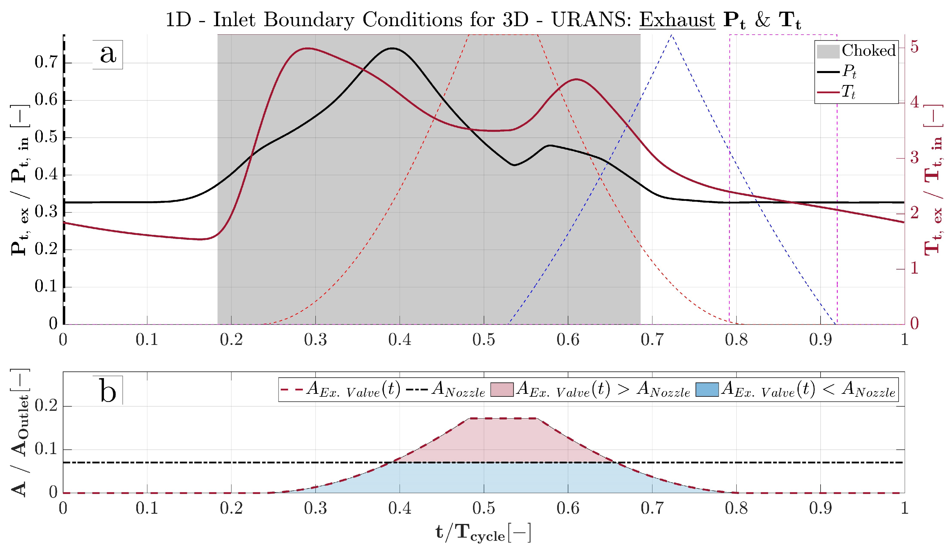
2.2.2. Transient Conditions of Exhaust System

The goal of the first part of this work was to retrieve sufficient total quantities downstream from the exhaust valves for the 3D transient numerical analysis of the exhaust system. After validating the model, the stagnation properties were derived and are depicted in Figure 6a. The exhaust system follows a “filling–emptying” process, which, of course, is the reverse “filling–emptying” process of the combustion chamber. When the exhaust valves are open, the stagnation pressure of the system rises, forcing the hot exhaust flow to pass through the plenum and the nozzle ($\frac{t}{T_{cycle}}=[0.18-0.5]$). By the time the intake valve opens ($\frac{t}{T_{cycle}}=[0.55-0.69]$), the temperature instantly rises and experiences a further increase during the scavenging process. A similar behaviour emerges for the stagnation pressure. However, while the valves are closed ($\frac{t}{T_{cycle}}>0.8$), the pressure reduces and approaches the atmospheric pressure. In fact, the gaps of the exhaust valves provide a continuous mass flow rate to the exhaust system.

It is clearly evident that the raised pressure ratio chokes the nozzle for almost half of the cycle. In parallel, the exhaust valves’ cross-sectional area is transient. When they are slightly open, they result in the minimum area of the system, controlling the chamber’s mass flow. When they are fully open, the nozzle’s throat is smaller (almost half of the valve’s nominal area) and takes control of the exhaust flow. This sequential change of the exhaust system’s controlling component, exhaust valves or nozzle, is presented in Figure 6b, where the y-abscissa is dimensionless with the help of the cross-sectional area of the exhaust plenum ($A_{Outlet})$.

On this point, it would be valuable to analyse the choice of the nozzle throat relative to the valves’ area. This subject has already been discussed by Boust et al. [34]. Nonetheless, it would be crucial to be mentioned again for the purposes of the future design of another exhaust system, such as the integration of CVC with HPT. The outlet system restriction (existing nozzle or future implemented IGVs) controls the scavenging process of the chamber when its area is smaller than that of the exhaust valves. It is useful to define $\Delta t_{Nozzle}$, the time window when the throat of the nozzle is smaller (pink shaded region in Figure 6b), than the resulting valves’ cross-sectional area. In the case of a small $\Delta t_{Nozzle}$, a larger mass flow rate is allowed to exit from the chamber during the scavenging process. This definitely helps the chamber to be better “cleaned”, increasing the combustion efficiency and reducing the cycle’s variability [33]. In addition, this hypothesis leads to a larger pressure gain inside the chamber. However, the exhaust valves control the exhaust system for a longer time window, and the outflow is expanded before entering into the exhaust plenum. Consequently, considerable expansion losses are induced on the outflow, which is guided to the nozzle. In conclusion, a larger nozzle throat (i.e., a small $\Delta t_{Nozzle}$) leads to a larger pressure gain inside the chamber but also leads to a smaller potential pressure gain to the exhaust plenum. On the other hand, if $\Delta t_{Nozzle}$ is large, the nozzle controls the outflow of the combustor for a longer time. Therefore, less mass flow exits during the scavenging process which means a larger fraction of residual burned gases inside the chamber. Thus, the aforementioned implications for combustion due to residuals are again dominant. The chamber’s pressure cannot reach the high levels of the other case having a lower pressure gain inside the chamber. Nevertheless, the burned gases flow and do not expand to the exhaust system when the out-take valves are open. In conclusion, a smaller nozzle throat (i.e., a large $\Delta t_{Nozzle}$) leads to a smaller pressure gain inside the chamber but also leads to a larger potential pressure gain in the exhaust plenum. This compromise between the effective pressure gain of the exhaust system and the combustion efficiency, which facilitates the disappearance of the cycle’s variation, should play a catalytic role for the future design of an efficient subsequent turbomachinery component coupled with a CVC.

3. 3D Transient Analysis of Exhaust System

In the second part of this work, the transient 3D simulation of the exhaust system is presented. The results of the reduced-order model are used as time-dependent spatially-averaged boundary conditions at the inlet of the exhaust. The commercial solver ANSYS™ FLUENT™ 2021 R1 [40] was employed to solve the required Steady and Unsteady Reynolds-Averaged Navier–Stokes (RANS and URANS) equations using a density-based implicit solver. First, the governing equations of the 3D solver are listed and described (Section 3.1). The flow domain, its boundary conditions, and the numerical setup of the simulation are presented in Section 3.2. The methodology used for the assessment of the periodic convergence of the simulation at the outflow is described in Section 3.3. In the end, the exhaust flow pattern is depicted considering one period of fluctuation in Section 3.4.

3.1. Governing Equations

Before describing the results of the 3D simulations obtained during the current study, the implementation of the flow equations in the solver is reported. URANS equations are discretized and solved in a finite-volume 3D solver. It should be underlined that the Einstein notation for the vectors of the Navier–Stokes equations is used. Moreover, the Reynolds averaging approach is applied to the Navier–Stokes and energy equations. As a consequence, the instantaneous field is expressed as the summation of the mean value and the fluctuating component for both scalars (e.g., $\varphi =\overline{\varphi }+{\varphi }^{\prime }$) and vectors (e.g., $u_i=\overline{u_i}+u_i^{\prime }$). Thus, by taking a time (or ensemble) average and dropping the overbar on the quantities except for products of fluctuating quantities, the URANS equations are reported in Equations (18)–(20).

$$\frac{\partial \rho }{\partial t}+\frac{\partial }{\partial x_i}\left(\rho u_i\right)=0$$

(18)

$$\frac{\partial }{\partial t}(\rho u_i)+\frac{\partial }{\partial x_j}(\rho u_i{u}_j)=-\frac{\partial p}{\partial x_i}+\frac{\partial }{\partial x_j}[\mu (\frac{\partial u_i}{\partial x_j}+\frac{\partial u_j}{\partial x_i}-\frac{2}{3}{\delta }_{ij}\frac{\partial u_l}{\partial x_l})]+\frac{\partial }{\partial x_j}(-\rho \overline{u_i^{\prime }{u}_j^{\prime }})$$

(19)

$$\frac{\partial }{\partial t}(\rho h_t)-\frac{\partial }{\partial t}(p)+\frac{\partial }{\partial x_j}(\rho u_j{h}_t)=\frac{\partial }{\partial x_j}(\lambda \frac{\partial T}{\partial x_j}-\rho \overline{u_j{h}_t})+\frac{\partial }{\partial x_j}[u_i({\tau }_{ij}-\rho \overline{u_i^{\prime }{u}_j^{\prime }})]$$

(20)

In the energy equation (Equation (20)), ${\tau }_{ij}$ is the molecular stress tensor of Equation (21), while $h_t$ is the total enthalpy given by Equation (22).

$${\tau }_{ij}=\mu (\frac{\partial u_i}{\partial x_j}+\frac{\partial u_j}{\partial x_i}-\frac{2}{3}{\delta }_{ij}\frac{\partial u_l}{\partial x_l})$$

(21)

$$h_t=h+\frac{1}{2}{u}_i{u}_i+k$$

(22)

In RANS calculations, the closure problem is faced when calculating the unknown term of the Reynolds stress tensor ($R_{ij}$) based on the eddy viscosity models:

$$R_{ij}=-\rho \overline{u_i^{\prime }{u}_j^{\prime }}={\mu }_t(\frac{\partial u_i}{\partial x_j}+\frac{\partial u_j}{\partial x_i})-\frac{2}{3}{\delta }_{ij}(\rho k+{\mu }_t\frac{\partial u_l}{\partial x_l})$$

(23)

Hence, the unknown term of the RANS equations is only the eddy viscosity ${\mu }_t$. The chosen turbulence model for this analysis is the standard k-$\omega$ model, in which the eddy viscosity is calculated as follows:

$${\mu }_t={\alpha }^{\ast }\frac{\rho k}{\omega }$$

(24)

In Equation (24), ${\mu }_t$ is a function of a corrective coefficient (${\alpha }^{\ast }$) for low Reynolds flow, density ($\rho$), turbulent kinetic energy (k), and specific dissipation rate ($\omega$). Hence, the final transport equations of the k-$\omega$ model are as follows:

$$\frac{\partial }{\partial t}(\rho k)+\frac{\partial }{\partial x_i}(\rho k{u}_i)=\frac{\partial }{\partial x_j}({\mathsf{\Gamma }}_k\frac{\partial k}{\partial x_j})+G_k-Y_k$$

(25)

$$\frac{\partial }{\partial t}(\rho \omega )+\frac{\partial }{\partial x_i}(\rho \omega u_i)=\frac{\partial }{\partial x_j}({\mathsf{\Gamma }}_{\omega }\frac{\partial \omega }{\partial x_j})+G_{\omega }-Y_{\omega }$$

(26)

The calculation of terms associated with generation $G_k$ and $G_{\omega }$ (due to mean velocity gradients), effective diffusivity ${\mathsf{\Gamma }}_k$ and ${\mathsf{\Gamma }}_{\omega }$, and dissipation $Y_k$ and $Y_{\omega }$ of turbulent kinetic energy and specific dissipation rate, respectively, can be found in [41]. By solving the transport equations of the turbulence model (Equations (25) and (26)), the eddy viscosity (Equation (24)) and the Reynolds stress (Equation (23)) can be calculated. As a consequence, the URANS equations (Equations (18) and (19)) accompanied by the energy Equation (Equation (20)) can specify the flow field of the domain for every instant of the analysis. In the end, the dynamic viscosity of Equations (19) and (20) is calculated using the Sutherland law:

$$\mu ={\mu }_0(\frac{T}{T_0}{)}^{3/2}\frac{T_0+S_0}{T+S_0}$$

(27)

where ${\mu }_0=1.716$×${10}^{-5}$ [kg/m $·$ s], $T_0=243.11$ [K], and $S_0=110.56$ [K].

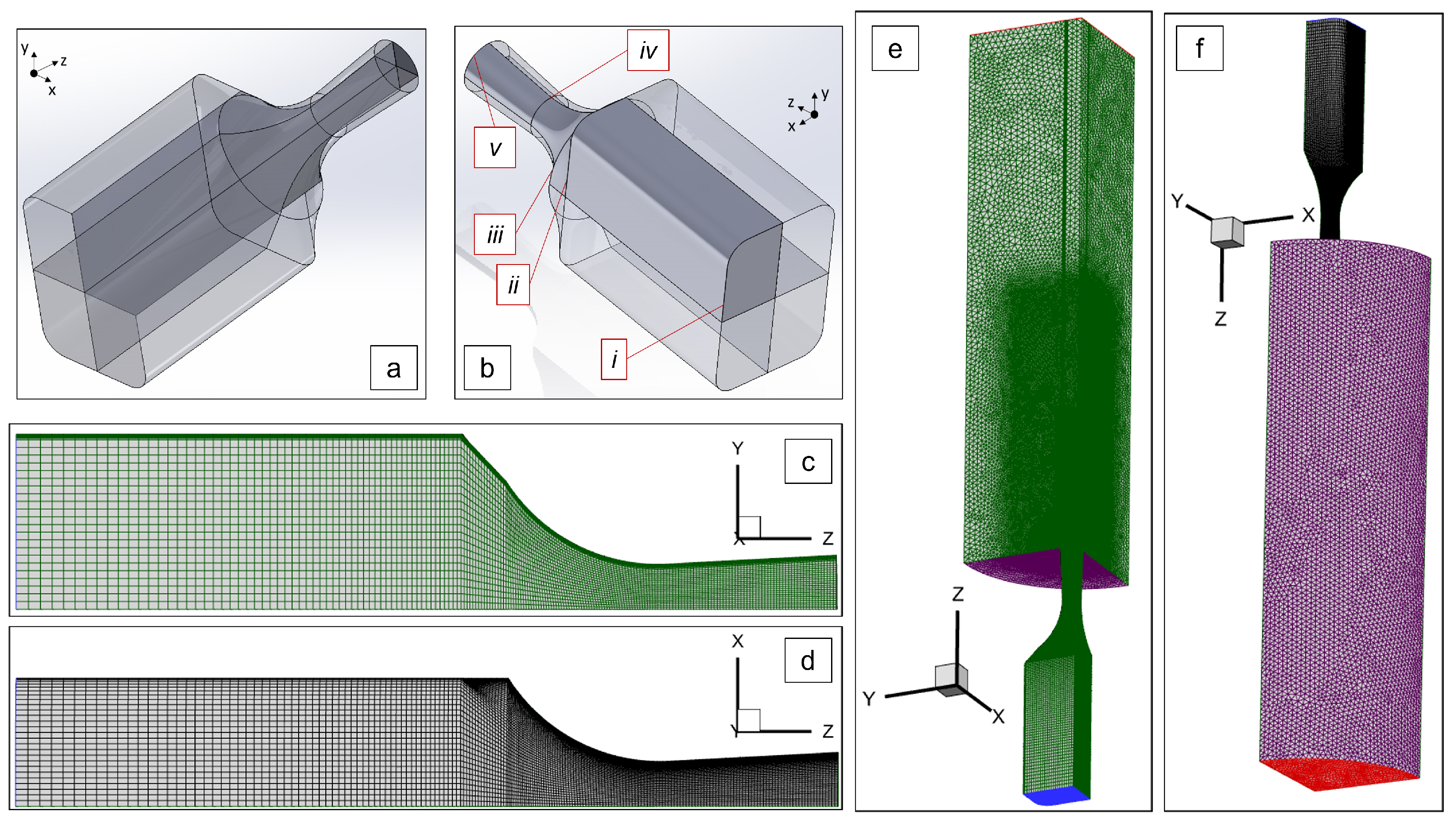
3.2. Numerical Setup

In Figure 7a,b the iso-views of the exhaust flow domain which consists of a rectangular plenum coupled with a transition duct that connects it with a circular converging–diverging nozzle are shown. As it can been seen, the domain can be separated into four identical volumes using the double symmetry of planes x-z and y-z. Therefore, the analysis can be performed on only one volume assuming a symmetric behaviour of the flow on these planes. Consequently, the computational cost is significantly reduced. In addition, Figure 7c,d present the mesh of the exhaust system which is constructed using tetrahedral elements placed on the z-axis. Moreover, 22 prismatic layers are stacked close to the viscous walls in order to properly resolve the viscous sub-layer preserving $y^{+}$ below 1. From Figure 7c to Figure 7f, different colours are used to highlight the selected boundary condition coherently with colours reported in

Table 4. Boundary conditions of domain. Colours correspond to Figure 7c–f.

Boundary Conditions
Type	Properties
Inlet	$P_{t,ex.}\left(t\right)$ and $T_{t,ex.}\left(t\right)$
Outlet	$P_{amb.}=1\left[atm\right]$
Symmetry	-
No - Slip Wall	Adiabatic
Free - Slip Wall	Adiabatic

, where the properties of the flow are also present.

An artificial exhaust plenum constituted by a quarter of the cylinder is positioned right after the exit of the nozzle, as shown in Figure 7e,f. The placement of this additional domain is useful to avoid spurious reflections of the outflow wave patterns backwards through the nozzle. In fact, if the outlet boundary section is positioned at the end of the nozzle, acoustic waves would be reflected into the nozzle. Hence, the plenum simulates the presence of ambient conditions without inserting non-physical pressure waves into the system.

The properties of the mesh are elected after performing a grid dependence analysis that consists of 3 steady CFD RANS simulations imposing the boundary conditions of the period’s instance that results in the maximum mass flow. In particular, the high pressure ratio leads to an over-expanded nozzle. The results of this analysis based on the theory of Roache [42] are presented in

Table 5. Grid dependency analysis.

Property	Grid	Refinement Ratio	GCI	Asymptotic Range of Convergence
$\dot{m}$	Coarse–Medium Medium–Fine	$1.261$ $1.260$	$0.745\%$ $0.474\%$	$1.0049$
M	Coarse–Medium Medium–Fine	$1.261$ $1.260$	$0.716\%$ $0.490\%$	$1.0037$
$T_t$	Coarse–Medium Medium–Fine	$1.261$ $1.260$	1.2 × ${10}^{-5}\%$ 6.2 × ${10}^{-6}\%$	$1.002$

. The properties of mass flow rate, mass flow-weighted average Mach number, and mass flow-weighted average stagnation temperature at the inlet of the nozzle (label “iii” in Figure 7b) were selected for the purpose of this study. The Grid Convergence Index (GCI) decreased from coarse–medium to medium–fine for the three properties providing values of the asymptotic range of convergence very close to 1.

The variation of the relative errors for the three properties at the inlet of the nozzle are plotted in a logarithmic scale in Figure 8. For each flow property, the values of the three grids are compared with the value obtained by the Richardson extrapolation. The mass flow rate and mass flow-weighted average stagnation temperature converge with an order higher than 2, while for the mass flow-weighted average Mach number, the order is $1.6$. Furthermore, the centre-line pressure ratio profiles $\pi$ from “i” to “v” (see Figure 7b) are reported for the three grids in Figure 9. As it can be observed, the position of the shock slightly changes from coarse to medium mesh while only the local $\pi$ value is modified by ≈3% when moving from medium to fine mesh. Based on the information provided, it can be concluded that the grid size of the medium meshed volume provides grid-independent results. The total amount of elements of the selected mesh is ≈4 × ${10}^6$.

The URANS equations were solved using a density-based implicit solver with a 2nd order accuracy. The medium was considered an ideal gas by imposing the cycle-averaged properties of the burned gases (${\overline{c}}_p=1367.785$ [J/(kg K)] and ${\overline{M}}_W=28.0808$ [kg/kmol]). The calculation using the 1D model showed a limited variation of the exhaust products’ properties ($\frac{\sigma \left(c_p\right)}{{\overline{c}}_p}=10$% and $\frac{\sigma \left(\gamma \right)}{\overline{\gamma }}=2$%). Hence, the assumption of constant thermodynamic properties of the exhaust products was made for the sake of calculation simplicity. Turbulence was calculated with the k-$\omega$ model proposed by Wilcox [41]. The operating frequency was 25 Hz ($T_{Cycle}=0.04$ s). Due to the rapid decrease in stagnation pressure, it was necessary to impose a variable time step during the computation, as reported in Figure 10. The analysis started with a coarse time step that guaranteed a numerical sampling frequency of $37.5$ kHz. Later, when the stagnation pressure was reduced, the numerical sampling frequency was increased up to 75 kHz. The following short recuperation of pressure allowed for analysing the development of the flow with a lower sampling frequency $37.5$ kHz, while, later, the analysis returned to 75 kHz. The end of the cycle was calculated with $37.5$ kHz. Such approach does not impact the accuracy of the computation but reduces the computational cost.

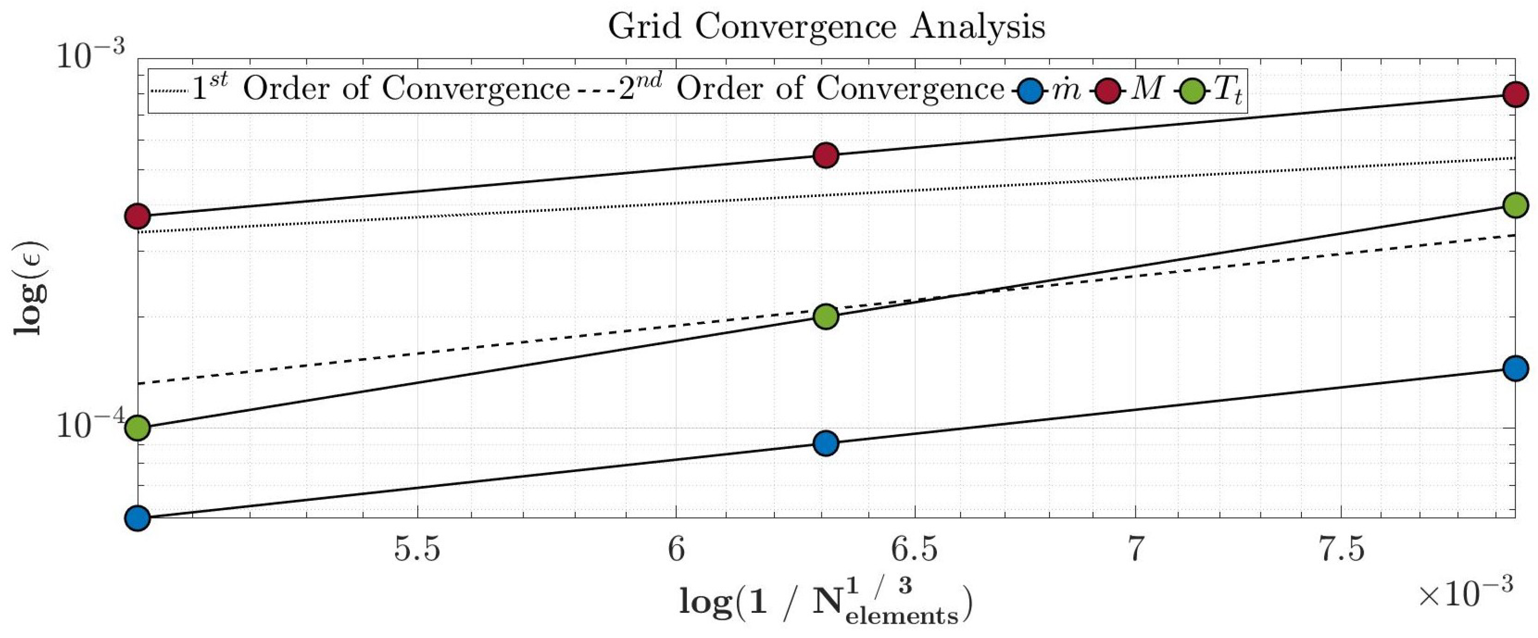
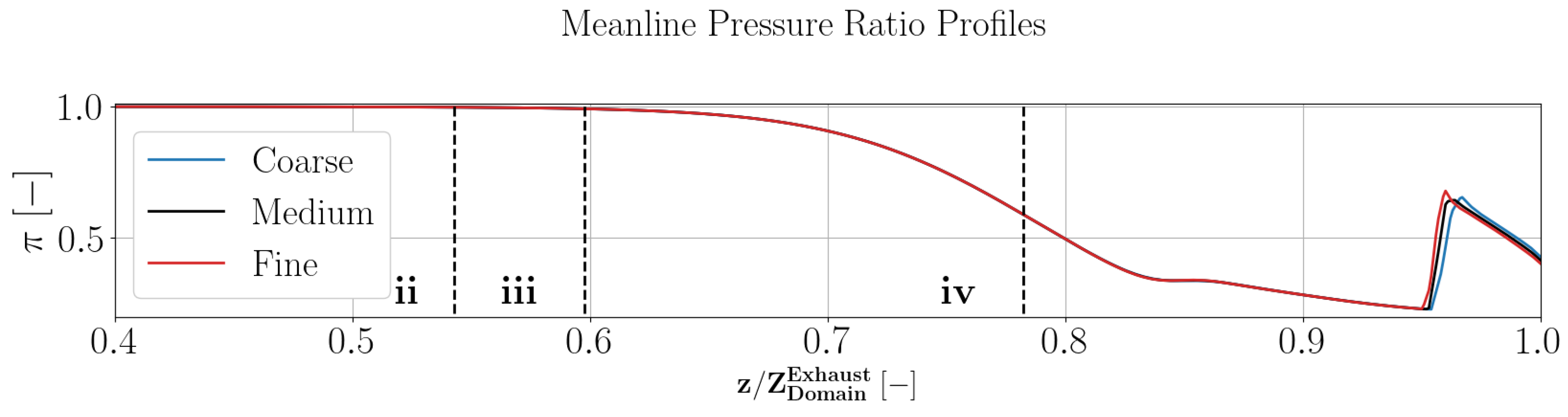
3.3. Periodic Convergence Criteria

Once the numerical scheme and the grid size of the domain is defined, a criterion of the convergence of the periodicity of the flow domain must also be determined. First, the simulation was initialized with the coarse frequency of $37.5$ kHz (cycle 0). Later, the simulation ran with the variable time step approach reported in Figure 10. Between the cycles, the cross-correlation of the mass flow rate, mass flow-weighted average Mach, and mass flow-weighted average stagnation temperature of the locations from “i” to “v” in Figure 7b was performed. Hence, the value of the normalised cross-correlation for a zero lag was calculated. The values of these properties are presented in accordance with the matrices in Equation (28).

$${\widehat{C}}_{\dot{m}}=\left[\begin{array}{c}{\left({\widehat{C}}_{\dot{m}}\right)}_i\\ {\left({\widehat{C}}_{\dot{m}}\right)}_{ii}\\ {\left({\widehat{C}}_{\dot{m}}\right)}_{iii}\\ {\left({\widehat{C}}_{\dot{m}}\right)}_{iv}\\ {\left({\widehat{C}}_{\dot{m}}\right)}_v\end{array}\right],{\widehat{C}}_M=\left[\begin{array}{c}{\left({\widehat{C}}_M\right)}_i\\ {\left({\widehat{C}}_M\right)}_{ii}\\ {\left({\widehat{C}}_M\right)}_{iii}\\ {\left({\widehat{C}}_M\right)}_{iv}\\ {\left({\widehat{C}}_M\right)}_v\end{array}\right],{\widehat{C}}_{T_t}=\left[\begin{array}{c}{\left({\widehat{C}}_{T_t}\right)}_i\\ {\left({\widehat{C}}_{T_t}\right)}_{ii}\\ {\left({\widehat{C}}_{T_t}\right)}_{iii}\\ {\left({\widehat{C}}_{T_t}\right)}_{iv}\\ {\left({\widehat{C}}_{T_t}\right)}_v\end{array}\right]$$

(28)

In Figure 11, the minimum, average, and maximum of each matrix are presented in the three graphs for four comparisons of the five cycles. In terms of mass flow, at the fifth cycle, the three properties of the normalised cross-correlation for zero lag are above $0.998$. The same is also true for the mass flow-weighted average Mach number and mass flow-weighted average stagnation temperature, corroborating the fact that the periodicity is established in the flow field for the fifth resolved period.

3.4. Results of URANS CFD

The transient inlet stagnation pressure of the system varies its operating conditions with time. The different conditions of the exhaust system are depicted in Figure 12. In Figure 12a, the intake properties of the system can be recognised. The stagnation pressure and temperature over the period are plotted, accompanied by the time window of the choked nozzle. Furthermore, five vertical coloured lines indicate the different analysed operating instances. In Figure 12b, the centre-line profile of the pressure ratio over the axial length of the nozzle for various time steps can be retrieved. Moreover, the locations of the inlet of the exhaust domain (i), inlet of the transition piece (ii), inlet of the nozzle (iii), throat of the nozzle (iv), and outlet of the nozzle (v) are presented in accordance with Figure 7b. Finally, in Figure 12c, the Mach number contour of the exhaust nozzle for these instances is presented.

Starting with $t_1$, the exhaust system is supplied by the very limited mass flow rate of the clearances of the exhaust valves. The pressure ratio profile is always higher than the critical pressure ratio (superimposed green curve on yellow curve of Figure 12b). As a result, the flow field of the exhaust nozzle is held at the subsonic operation. As the combustion occurs and the exhaust valves start to open, the inlet stagnation properties are raised. This leads to the sufficient supply of the inlet total pressure, which results in a lower pressure ratio than the critical one. Moreover, the outlet pressure very quickly decreases below the ambient condition, creating an over-expanded nozzle. The time instant $t_2$ provides a pressure profile profoundly lower than the critical pressure ratio after the throat position. In addition, the associated flow field of the oblique shocks, Mach discs, and expansion waves are evident in Figure 12c. Afterwards, the supplying stagnation pressure starts reducing, and the over-expanded profile of the nozzle flinches upstream ($t_3$). However, the opening of the intake valves ($t_4$) ensures that the nozzle remains in the choked operating point for another 15% of the cycle. In the end, the exhaust closes the valves, again allowing for a significantly smaller mass flow rate to the system, and the nozzle returns to the non-choked operating point. The return to steadiness at the exhaust can be seen at $t_5$.

On that point, it would be very useful to define some metrics of evaluation for the exhaust system for the fifth analysed cycle. The property that is chosen to be used is the stagnation pressure. Apparently, in terms of efficiency, the characterisation of the cycle-averaged stagnation pressure losses (${\overline{\zeta }}_{P_t}$) through each part of the exhaust system should be performed. In addition, the level of excitation or attenuation of the fluctuations of the CVC exhaust’s total pressure it should be calculated for each of the downstream parts. Therefore, the reduced range $\widehat{R}$ of a signal is used here, which is computed by the division of the range with its average. As a result, the difference between inlet and outlet in terms of the reduced range can give the damping factor $D_{\widehat{R}}$, as was introduced by Liu et al. [25]. If this factor is positive, the signal is attenuated. On the other hand, if it is negative, the signal is excited. Consequently, the losses and oscillation characterisation of a component can be performed using Equation (29).

$${\overline{\zeta }}_{P_t}=\frac{{[\overline{P_t}]}_{out}-{[\overline{P_t}]}_{in}}{{[\overline{P_t}]}_{in}}\&\widehat{R}=\frac{Range\left(P_t\right)}{\overline{P_t}}\to D_{\widehat{R}}=\frac{{\widehat{R}}_{Inlet}-{\widehat{R}}_{Outlet}}{{\widehat{R}}_{Inlet}}$$

(29)

The aforementioned cycle evaluations of the flow field can be found in Figure 13. In Figure 13a, the damping factor of every part of the exhaust system is depicted. Right afterward, the cumulative damping factor of every component is presented in Figure 13b. In particular, for acquiring the latter, values of mass flow weighted-average stagnation pressure at every exit are compared with one of the inlets of the domain (plenum inlet “i” in Figure 7b). The third graph presents the losses’ characterisation of every component, and the last graph presents the cumulative losses’ evaluation. First of all, it is clear that the plenum excites the stagnation pressure. A negligible contribution to excitation occurs from the transition piece as well. However, the nozzle provides an attenuation of the stagnation pressure, in particular to the diverging part. On the other hand, negligible losses are inserted to the system by the plenum and the transition piece. The convergent part increases the losses, while the majority of losses occur in the diverging part. It can be concluded that the attenuation of the stagnation pressure takes place through the intense change in the kinetic energy of the medium. The subsonic acceleration by the restriction of the area seems to be the less effective way but also the method with the less induced losses. Nevertheless, the system reaches 8% of attenuation by transiently choking the flow in the divergent component, imposing the highest level of losses in the exhaust part. A final metric of the performance of the exhaust system is the damping efficiency defined in Equation (30).

$${\eta }_D=1-\frac{|{\overline{\zeta }}_{P_t}|}{D_{\widehat{R}}}$$

(30)

The convergent part is characterised by $32.40$% of efficiency, while the divergent part provides an efficiency of $60.10$%. It is demonstrated that the divergent nozzle damps the stagnation pressure more with less relative losses with respect to the convergent part for one cycle. This underlines the effectiveness of the shock wave patterns and the expansion of the flow. On the one hand, the superiority of the component is clear, but on the other hand, this claim should be examined in-depth. First of all, the kinetic energy of the entrance of the two components is not the same. Moreover, the flow after the divergent nozzle is expanded. Thus, it loses its potential energy, which can be used for any subsequent component capable to extract work by it, like a turbine module. This is certainly crucial and points out the major role of the maximisation of the attenuation with respect to the produced losses before the flow expansion. It is quite evident that the expansion is the better way to attenuate the flow field pulsation, but the proper subsonic acceleration is the spotlight of the future redesign of the exhaust system coupled with IGVs. For an HPT stage, the attenuation of the stagnation pressure before the throat of IGVs is a key parameter for the proper functioning of the stage.

4. Conclusions

This analysis is the first attempt to present the complex outflow of the CVC and aimed at paving the way for the redesign of an efficient exhaust system which will connect a CVC chamber with a conventional HPT stage. A 1D model for a novel PGC and the 3D flow field analysis of the exhaust system are presented. The necessary modifications to the model to reproduce the particular case of a CVC chamber are mentioned. The calibration of the system, in terms of discharge coefficients, non-dimensional burning rate, and heat losses, is accomplished. Afterwards, the obtained result of the chamber’s pressure is compared to the experimental data. The simulation falls within the experimental range and agrees with high accuracy to the majority of the time periods at the ninth experimental cycle. Furthermore, the retrieved stagnation properties after the exhaust valves for a CVC are presented for the first time in the literature, and they are thoroughly discussed. At the end of this part, the major role of the ratio between the throat area of the exhaust component and the transient cross-section of out-take valves is explained.

In the second part, the flow domain of the exhaust system and its boundary condition are introduced. The periodicity is proven as being established in the domain after the fifth cycle by calculating the normalised cross-correlation of the CFD transient signals for zero lag. The nozzle experiences a “filling–emptying” process passing from the subsonic regime to the choked over-expanded operating point. The losses and the oscillation characterisation are chosen as a metric of the outflow with this PGC. It is proven that the flow expansion provides a relatively higher attenuation compared to the subsonic acceleration.

The interest of the propulsion research community revolves around the challenges and the applications of PGC systems. The presented work attempts to contribute to the investigation of these unconventional machines, as valuable conclusions are derived for the performance of the CVC exhaust system. This is the first time that the outlet conditions of this PGC prototype are retrieved. The 1D model of the ensemble test rig is validated, and the spatial average time-resolved exhaust conditions are thoroughly described. These conditions will contribute to the upcoming design of an exhaust system which will focus on the integration of a CVC with an HPT stage. The selection of the exhaust system restriction area is the second major finding of the present work. The existing nozzle throat or future IGV throats should be carefully elected relative to the valve’s transient area. On the one hand, if the exhaust system throat is relatively small, it will control the scavenging process of the combustion chamber and, therefore, its performance for a long time of the cycle. On the other hand, if it is quite large and facilitates the scavenging process, the flow will be driven inside the exhaust plenum with considerable expansion losses. Consequently, it will be necessary to perform an investigation on the detection of the optimum ratio between the exhaust valve’s throat area and the restriction area of the outlet system. The last part of this work unveils interesting findings relevant to the weakening of a CVC pulsating outflow. The attenuation of the mass flow-weighted average total pressure signal by expansion at the divergent part is more efficient than the damping by subsonic acceleration at the convergent part. Nonetheless, the attenuation of the flow field before its expansion is of essence for a gas turbine cycle. Therefore, efforts should be concentrated on increasing the damping efficiency of the upstream subsonic acceleration for future integrations with an HPT. The attenuation of the flow with less produced entropy before its expansion is more essential for the proper functioning of the stage, as the extraction work of a turbine is based on the potential energy of the medium.

References

1. Stefanizzi, M.; Capurso, T.; Filomeno, G.; Torresi, M.; Pascazio, G. Recent Combustion Strategies in Gas Turbines for Propulsion and Power Generation toward a Zero-Emissions Future: Fuels, Burners, and Combustion Techniques. Energies 2021, 14, 6694. [Google Scholar] [CrossRef]
2. Perkins, H.D.; Paxson, D.E. Summary of Pressure Gain Combustion Research at NASA; Technical Report, NASA TM-2018-219874; NASA: Washington, DC, USA, 2018.
3. Holzwarth, H. Rotary Combustion Engine. U.S. Patent 783,434, 28 February 1905. [Google Scholar]
4. Glassman, I.; Yetter, R.A.; Glumac, N.G. Flame phenomena in premixed combustible gases. In Combustion, 5th ed.; Academic Press: Waltham, MA, USA, 2015; Chapter 4; pp. 147–254. [Google Scholar] [CrossRef]
5. Ciccarelli, G.; Dorofeev, S. Flame Acceleration and Transition to Detonation in Ducts. Prog. Energy Combust. Sci. 2008, 34, 499–550. [Google Scholar] [CrossRef]
6. Wolański, P. Detonative Propulsion. Proc. Combust. Inst. 2013, 34, 125–158. [Google Scholar] [CrossRef]
7. Nordeen, C.A. Concepts and Definitions: Efficiency of detonation. In Thermodynamics of a Rotating Detonation Engine; University of Connecticut: Storrs, CT, USA, 2013; Chapter 1; pp. 10–15. [Google Scholar]
8. Heiser, W.H.; Pratt, D.T. Thermodynamic Cycle Analysis of Pulse Detonation Engines. J. Propuls. Power 2002, 18, 68–76. [Google Scholar] [CrossRef]
9. Stathopoulos, P.; Vinkeloe, J.; Paschereit, C.O. Thermodynamic Evaluation of Constant Volume Combustion for Gas Turbine Power Cycles. In Proceedings of the Numerical Set Updings of the 11th International Gas Turbine Congress, Tokyo, Japan, 15–20 November 2015; pp. 15–20. [Google Scholar]
10. Sousa, J.; Paniagua, G.; Collado Morata, E. Thermodynamic Analysis of a Gas Turbine Engine with a Rotating Detonation Combustor. Appl. Energy 2017, 195, 247–256. [Google Scholar] [CrossRef]
11. Neumann, N.; Peitsch, D. Potentials for Pressure Gain Combustion in Advanced Gas Turbine Cycles. Appl. Sci. 2019, 9, 3211. [Google Scholar] [CrossRef]
12. Anand, V.; Gutmark, E. A Review of Pollutants Emissions in Various Pressure Gain Combustors. Int. J. Spray Combust. Dyn. 2019, 11, 175682771987072. [Google Scholar] [CrossRef]
13. Akbari, P.; Nalim, R.; Mueller, N. A Review of Wave Rotor Technology and Its Applications. J. Eng. Gas Turbines Power 2006, 128, 717–735. [Google Scholar] [CrossRef]
14. Roy, G.; Frolov, S.; Borisov, A.; Netzer, D. Pulse Detonation Propulsion: Challenges, Current Status, and Future Perspective. Prog. Energy Combust. Sci. 2004, 30, 545–672. [Google Scholar] [CrossRef]
15. Bobusch, B.C.; Berndt, P.; Paschereit, C.O.; Klein, R. Shockless Explosion Combustion: An Innovative Way of Efficient Constant Volume Combustion in Gas Turbines. Combust. Sci. Technol. 2014, 186, 1680–1689. [Google Scholar] [CrossRef]
16. Ma, J.Z.; Luan, M.Y.; Xia, Z.J.; Wang, J.P.; Zhang, S.j.; Yao, S.b.; Wang, B. Recent Progress, Development Trends, and Consideration of Continuous Detonation Engines. AIAA J. 2020, 58, 4976–5035. [Google Scholar] [CrossRef]
17. Lu, F.K.; Braun, E.M. Rotating Detonation Wave Propulsion: Experimental Challenges, Modeling, and Engine Concepts. J. Propuls. Power 2014, 30, 1125–1142. [Google Scholar] [CrossRef]
18. Hishida, M.; Fujiwara, T.; Wolanski, P. Fundamentals of Rotating Detonations. Shock Waves 2009, 19, 1–10. [Google Scholar] [CrossRef]
19. Lee, J.H.S. Introduction: The detonation Structure. In The Detonation Phenomenon, 1st ed.; Cambridge University Press: New York, NY, USA, 2008; Chapter 1; pp. 11–12. [Google Scholar] [CrossRef]
20. Fernelius, M.; Gorrell, S.E.; Hoke, J.; Schauer, F. Effect of Periodic Pressure Pulses on Axial Turbine Performance. In Proceedings of the 49th AIAA/ASME/SAE/ASEE Joint Propulsion Conference, San Jose, CA, USA, 15–17 July 2013; p. 3687. [Google Scholar] [CrossRef]
21. Fernelius, M.H.; Gorrell, S.E. Predicting Efficiency of a Turbine Driven by Pulsing Flow. In Proceedings of the Volume 2A: Turbomachinery, Charlotte, NC, USA, 26–30 June 2017; p. V02AT40A008. [Google Scholar] [CrossRef]
22. Fernelius, M.H.; Gorrell, S.E. Mapping Efficiency of a Pulsing Flow-Driven Turbine. J. Fluids Eng. 2020, 142, 061202. [Google Scholar] [CrossRef]
23. Fernelius, M.H.; Gorrell, S.E. Design of a Pulsing Flow Driven Turbine. J. Fluids Eng. 2021, 143, 041501. [Google Scholar] [CrossRef]
24. Paniagua, G.; Iorio, M.; Vinha, N.; Sousa, J. Design and Analysis of Pioneering High Supersonic Axial Turbines. Int. J. Mech. Sci. 2014, 89, 65–77. [Google Scholar] [CrossRef]
25. Liu, Z.; Braun, J.; Paniagua, G. Performance of Axial Turbines Exposed to Large Fluctuations. In Proceedings of the 53rd AIAA/SAE/ASEE Joint Propulsion Conference, Atlanta, GA, USA, 10–12 July 2017; p. 4817. [Google Scholar] [CrossRef]
26. Liu, Z.; Braun, J.; Paniagua, G. Integration of a Transonic High-Pressure Turbine with a Rotating Detonation Combustor and a Diffuser. Int. J. Turbo Jet-Engines 2023, 40, 1–10. [Google Scholar] [CrossRef]
27. Liu, Z.; Braun, J.; Paniagua, G. Thermal Power Plant Upgrade via a Rotating Detonation Combustor and Retrofitted Turbine with Optimized Endwalls. Int. J. Mech. Sci. 2020, 188, 105918. [Google Scholar] [CrossRef]
28. Ni, R.H.; Humber, W.; Ni, M.; Sondergaard, R.; Ooten, M. Performance Estimation of a Turbine Under Partial-Admission and Flow Pulsation Conditions at Inlet. In Proceedings of the Volume 6C: Turbomachinery, San Antonio, TX, USA, 3–7 June 2013; p. V06CT42A019. [Google Scholar] [CrossRef]
29. Xisto, C.; Petit, O.; Grönstedt, T.; Rolt, A.; Lundbladh, A.; Paniagua, G. The Efficiency of a Pulsed Detonation Combustor–Axial Turbine Integration. Aerosp. Sci. Technol. 2018, 82–83, 80–91. [Google Scholar] [CrossRef]
30. Naples, A.; Hoke, J.; Battelle, R.; Schauer, F. T63 Turbine Response to Rotating Detonation Combustor Exhaust Flow. J. Eng. Gas Turbines Power 2019, 141, 021029. [Google Scholar] [CrossRef]
31. Boust, B.; Michalski, Q.; Bellenoue, M. Experimental Investigation of Ignition and Combustion Processes in a Constant-Volume Combustion Chamber for Air-Breathing Propulsion. In Proceedings of the 52nd AIAA/SAE/ASEE Joint Propulsion Conference, Salt Lake City, UT, USA, 25–27 July 2016; p. 4699. [Google Scholar] [CrossRef]
32. DS/EN ISO 9300; Measurement of Gas Flow by Means of Critical Flow Venturi Nozzles. Dansk Standard; American National Standards Institute: New York, NY, USA, 1987.
33. Labarrere, L.; Poinsot, T.; Dauptain, A.; Duchaine, F.; Bellenoue, M.; Boust, B. Experimental and Numerical Study of Cyclic Variations in a Constant Volume Combustion Chamber. Combust. Flame 2016, 172, 49–61. [Google Scholar] [CrossRef]
34. Boust, B.; Bellenoue, M.; Michalski, Q. Pressure Gain and Specific Impulse Measurements in a Constant-Volume Combustor Coupled to an Exhaust Plenum. In Proceedings of the Active Flow and Combustion Control 2021, Berlin, Germany, 28–29 September 2021; pp. 3–15. [Google Scholar] [CrossRef]
35. Gallis, P.; Misul, D.A.; Salvadori, S.; Bellenoue, M.; Boust, B. Development and Validation of a 0-D/1-D Model to Evaluate Pulsating Conditions from a Constant Volume Combustor. In Proceedings of the Joint Meeting of International Workshop on Detonation for Propulsion (IWDP) and International Constant Volume and Detonation Combustion Workshop (ICVDCW), Berlin, Germany, 15–19 August 2022. [Google Scholar] [CrossRef]
36. GT-SUITE Flow Theory Manual; GT-Power: Malvern, PA, USA, 2020.
37. Courant, R.; Friedrichs, K.; Lewy, H. On the Partial Difference Equations of Mathematical Physics. Ibm J. Res. Dev. 1967, 11, 215–234. [Google Scholar] [CrossRef]
38. Ghojel, J.I. Review of the Development and Applications of the Wiebe function: A Tribute to the Contribution of Ivan Wiebe to Engine Research. Int. J. Engine Res. 2010, 11, 297–312. [Google Scholar] [CrossRef]
39. Labarrere, L. Un outil de simulation 0D pour la combustion isochore: CVC0D—Modélisation de la combustion. In Etude Théorique et Numérique de la Combustion à Volume Constant Appliquée à la Propulsion; Institut National Polytechnique de Toulouse: Toulouse, France, 2016; Chapter 3; p. 51. [Google Scholar]
40. Ansys Fluent Theory Guide 2021 R1; ANSYS Inc.: Canonsburg, PA, USA, 2021.
41. Wilcox, D.C. Formulation of the k-w Turbulence Model Revisited. AIAA J. 2008, 46, 2823–2838. [Google Scholar] [CrossRef]
42. Roache, P.J. Verification of Codes and Calculations. AIAA J. 1998, 36, 696–702. [Google Scholar] [CrossRef]
Figure 1. CVC configuration and equivalent 1D model.
Energies 17 01191 g001
Figure 2. Operating description of model and calibration of a. discharge coefficients and b. burning rate.
Energies 17 01191 g002
Figure 3. Vertical and lateral gap profiles of the exhaust valves.
Energies 17 01191 g003
Figure 4. Sequential operation of inlet (blue) and outlet (red) rotary valves.
Energies 17 01191 g004
Figure 5. Validation of 1D model with experimental chamber’s pressure: (a) Comparison of experimental and model pressure, (b) Comparison of model with experimental limits and (c) Comparison of 9th experimental cycle with the model.
Energies 17 01191 g005
Figure 6. Stagnation Properties after the exhaust valves (a) and cross-area evolution of the exhaust system (b).
Energies 17 01191 g006
Figure 7. Flow domain and simulation mesh: (a) Exhaust system ensemble flow domain—view 1, (b) Exhaust system ensemble flow domain—view 2, (c) Exhaust system grid—view 1, (d) Exhaust system grid—view 2, (e) Exhaust system with artificial plenum grid—view 1 and (f) Exhaust system with artificial plenum grid—view 2. For (b) the symbols specify the locations of Inlet of Domain (i), Inlet of transition part (ii), Inlet of nozzle (iii), Throat of nozzle (iv) and Outlet of nozzle (v).
Energies 17 01191 g007
Figure 8. Variation of mass flow, Mach and total temperature errors with grid refinement.
Energies 17 01191 g008
Figure 9. Pressure Ratio center-line profiles of grid dependency analysis.
Energies 17 01191 g009
Figure 10. Variable time step selection over boundary conditions.
Energies 17 01191 g010
Figure 11. Cross-correlation of transient CFD signals for mass flow rate (a), mass flow—weighted Mach number (b) and mass flow—weighted total temperature (c).
Energies 17 01191 g011
Figure 12. Variable operating conditions of exhaust system: (a) Transient inlet boundary conditions of flow domain, (b) Center-line profile of pressure ratio of domain and (c) Mach number contour of exhaust nozzle for time moments t 1 , t 2 , t 3 , t 4 and t 5 .
Energies 17 01191 g012
Figure 13. Losses and oscillations’ characterisation of exhaust system: (a) Damping factor, (b) Cumulative damping factor, (c) Total pressure losses and (d) Cumulative total pressure losses.
Energies 17 01191 g013