Abstract
In order to solve the risk of transient voltage instability caused by the increasing proportion of new energy represented by photovoltaic (PV) and dynamic load in the power grid, a dynamic reactive power compensation device configuration method with high-permeability PV is proposed considering transient voltage stability. Firstly, a typical reactive power compensation device configuration is constructed, and evaluation indexes based on transient voltage disturbance and transient voltage peak are proposed. The static index based on complex network characteristics and the dynamic index based on sensitivity theory are used to guide the candidate nodes of dynamic reactive power compensation. Secondly, when reactive power capacity is configured, a differentiated dynamic reactive power compensation optimization model is established, and the multi-objective marine predator algorithm is used to solve the configured capacity, aiming to improve the transient voltage stability at the lowest reactive power investment cost. The final configuration scheme is selected by using the improved entropy weight ideal solution sorting method. Finally, the simulation results of the improved IEEE39-node system verify the effectiveness of the proposed method.
1. Introduction
Since the advent of the 21st century, the promotion of scientific and technological progress, along with the increasing demand for electric energy and evolving societal needs, have led to a growing proportion of motor-characteristic loads in power systems [1,2,3,4]. Furthermore, rapid advancements in new renewable energy applications within power grids, particularly PV, have exacerbated the issue of transient voltage stability [5,6,7,8]. To address this challenge effectively, it is crucial to employ reactive power compensation devices. Dynamic reactive power compensation devices can swiftly respond to grid failures by ensuring that system bus voltages remain within normal ranges while preventing severe transient voltage drops or overvoltages. In order to fully harness the benefits offered by dynamic reactive power compensation devices, careful consideration must be given to selecting appropriate installation sites as well as determining suitable installation types and capacities at different locations [9,10,11,12].
The selection of an appropriate installation location and type of dynamic reactive power compensation device is a fundamental aspect of reactive power planning. Most installation points are determined based on measures related to static voltage stability, such as the U-Q curve method [13], branch and bound method [14], the preselection method considering contingent conditions [15], and the method aimed at improving the reactive power margin of nodes [16]. However, these methods primarily focus on a single aspect and do not consider the dynamic characteristics of loads with induction motors or account for the compensation effect on transient voltage stability in the entire power system after compensation. Ref. [17] proposes an enhanced track sensitivity index approach to determine compensation locations; however, this method requires extensive calculations for large-scale power systems, resulting in redundant results without considering the rationality of actual compensation point locations. Furthermore, existing configuration schemes only consider final compensation effects without addressing economic considerations. In terms of reactive power device configuration, most methods employ a single compensator without analyzing different compensators’ characteristics or evaluating whether combining multiple compensators would yield better and more cost-effective results [18,19,20,21]. Therefore, previous studies on the location selection of dynamic reactive power compensation devices mainly focused on static stability in considering the stability of the system and did not consider the dynamic characteristics of fast-response devices such as induction motors. When the concept of sensitivity is used to select the installation bus of dynamic reactive power compensation device, the redundancy of sensitivity in large system is not considered. In the selection of the type of dynamic reactive power compensation device, there are no comprehensive advantages of different devices when it comes to carrying out differential reactive power compensation, and there is a single compensation device. In view of the above problems, this paper has made improvements in the following aspects: This paper mainly studies the transient stability of the system with photovoltaic and induction motor load and plans the photovoltaic output scenario based on the scenario probability theory. Before calculating the sensitivity of compensating dynamic reactive power compensation equipment at different busbars of a large system, the original system is modeled using complex network theory, and the unnecessary nodes are screened by using the complex network characteristic comprehensive index, which reduces the redundancy of location selection. The differential reactive power compensation model is established, and the dynamic reactive power compensation device is selected while reasonably considering the difference in performance and cost between STATCOM (STATic synchronous COMpensator) and SVC (Static Var Compensator).
In terms of determining the capacity of the reactive power compensation device, the core problem of dynamic reactive power planning, most of the existing indicators for maintaining the transient voltage stability of the power system only consider the voltage instability caused by substantial voltage reduction, and do not consider the photovoltaic units in the power system containing new energy units, such as photovoltaic units, due to the lack of high voltage crossing capacity. When transient overvoltage occurs, some units are taken off the grid and the whole power system voltage collapses. Ref. [22] proposed the voltage stability index, which is based on the Euclidean distance of the measured voltage vector curve, is to be utilized for the real-time monitoring of voltage. Ref. [23] proposed a dynamic reactive power source planning voltage stability analysis method to solve the evaluation problem of fault-induced delayed voltage recovery (FIDVR) mitigation technology. After considering the transient voltage recovery and dynamic characteristics of the dynamic reactive power compensation device, ref. [24] established a multi-objective optimization model with the minimum voltage deviation of the bus and the minimum installed capacity of the compensation device after the fault is cleared. Ref. [25] proposes a reactive power compensation device configuration method that takes into account both the static and transient voltage stability of the system. Ref. [26] takes the fault limit removal time as an index to reflect the transient voltage stability of each node of the system. Ref. [27] proposed a transient voltage severity index composed of the transient voltage deviation index. However, due to the large voltage instability margin set, the evaluation time is too short, and the results have significant errors. Therefore, the main limitations of previous studies on the capacity determination of dynamic reactive power compensation devices are as follows: In the power system of the main study, systems equipped with new energy units were not considered, such as systems containing a high proportion of photovoltaic units. Therefore, in the setting of the transient voltage stability index, the transient overvoltage of the bus bar where the photovoltaic unit is located is not involved. The research on the transient voltage stability index is not mature. Under the background of the increasing proportion of photovoltaics in the power grid, this paper innovatively defines the transient voltage stability index, including the global transient voltage disturbance index and the global voltage peak index. Global consideration can reduce the memory of data transmission during the time domain simulation and optimization operation.
To address the aforementioned issues, this paper proposes a method for configuring a dynamic reactive power compensation device to ensure transient voltage stability in PV systems with uncertainty. Section 2 of this paper introduces the voltage stability range and transient overvoltage mechanism in high-permeability PV power grids and determines the typical output scenario of photovoltaics. In Section 3, an evaluation index for transient voltage stability is established as the basis, incorporating both static location methods considering comprehensive indices of complex network characteristics and dynamic location methods considering sensitivity concepts. This enables differential compensation by the compensation device. Section 4 of this paper establishes a model for allocating reactive power capacity that considers both transient voltage stability and economic cost. The multi-objective marine predator algorithm is employed to solve this model, resulting in a Pareto solution set. By utilizing an improved technique for order preference by similarity to ideal solution (TOPSIS) method, score values are calculated for different configuration schemes based on various indexes, ultimately leading to selection of the optimal configuration scheme. In Section 5, the proposed configuration method in the improved IEEE39 nodes is validated using Matlab R2020b and PSAT 2.1.11.
2. Transient Analysis of a PV Grid-Connected System and Typical Scene Construction
2.1. PV Grid-Connected System Voltage Requirements
The state has put forward the following corresponding assessment standards for PV new energy grid-connected PV units with low voltage crossing operation requirements: when the PV power station voltage drops to 0 p.u., the PV power station should be able to run 0.15 s without off-grid; the voltage runs no less than 0.20 p.u. during the period from 0.15 s to 0.625 s; during the period from 0.625 s to 2 s, the voltage track is required to run continuously at the top left of the boundary without off-grid, otherwise it will be cut out from the grid; after 2 s, the voltage is required to run continuously no less than 0.9 p.u. High voltage crossing operation requirements: at least 10 s of continuous operation between 1.1 p.u. and 1.2 p.u., and at least 0.5 s of continuous operation between 1.2 p.u. and 1.3 p.u. [28]. The high/low voltage crossing standard requirements for photovoltaic power stations are shown in Figure 1.

Figure 1.
PV grid-connected high/low voltage crossing standards.
2.2. Generation Mechanism of Transient Overvoltage in PV Grid-Connected System
The transient overvoltage of the system is influenced by the current control speed of the PV unit. In the case of a short-circuit fault in the system, the PV unit enters a low-voltage crossing state, leading to an increase in reactive current and a decrease in active current. After clearing the fault, it takes several hundred seconds for the PV unit to withdraw reactive current and restore active current to its pre-fault state, resulting in an occurrence of excessive reactive power phenomenon.
Secondly, the capacitive reactive power control performance of the reactive power compensation device will also impact the system’s transient overvoltage. For instance, in the case of a deployed dynamic Var Compensator SVC, when a short-circuit fault occurs within the system, the voltage at the access point rapidly falls below the voltage control range. All thyristor-controlled reactors cease consuming reactive power while all capacitors discharge a significant amount of reactive power. Once the fault is cleared, there is a swift recovery in access point voltage. However, due to slightly slower reduction speed of capacitor’s reactive power output compared to voltage rise speed, the SVC injects excessive capacitive reactive power into the system after fault clearance, resulting in a transient overvoltage phenomenon caused by an excess of reactive power [29].
2.3. Construct Typical Scenario of PV Uncertainty
During the configuration of a dynamic reactive power compensation device, the uncertainty of PV output in the system will impact the configuration capacity. If the PV permeability is low, it can be compensated according to traditional methods for dynamic reactive power allocation, as it has minimal influence on the final outcome. However, when the PV permeability is high, relying solely on traditional thinking becomes overly idealized and inappropriate for addressing uncertainties in actual processes, leading to significant errors. Therefore, this paper constructs typical scenarios for high-permeability photovoltaics based on scenario probability theory to accurately characterize their inherent uncertainties [30].
The output of the PV generator set is dependent on the solar irradiance G, which follows a lognormal distribution. Its probability density function can be described as:
where fG(G) is the probability density function of solar irradiance. G is solar irradiance. Sigma is the standard deviation. µ is the mean value. The expressions of σ and µ are shown in Equations (2) and (3).
where V is the variance of the variable obeying lognormal distribution. M is the mean of the variable that follows a lognormal distribution.
The relationship between the output power of PV systems, denoted as Pp, and solar irradiance G can be described as follows:
where Gs is the solar irradiance under standard environment. Rc is a specific solar irradiance, and Pn is the rated output power of PV.
The typical PV scenarios are categorized into PV.1–PV.3 based on the output range, as per Formula (4). The probability of PV units operating in different scenarios is expressed by Formula (5), Formula (6), and Formula (7), respectively.
where PPV.a (a = 1, 2, 3) is the probability of the PV unit running under the typical scenario PV.a.
The output power of PV units in each typical scenario is considered as the output size of different scenarios in this paper. Therefore, the output power of PV units operating in the typical scenarios PV.1–PV.3 is as follows:
where PpPV.a (a = 1,2,3) is the output power of the PV unit operating in a typical scenario PV.a.
In practical engineering applications, fine-setting Rc values can be used to further divide typical scenes into smaller ones, enabling a more accurate reflection of the impact of varying degrees of high-permeability PV on the configuration results of dynamic reactive power compensation devices. The specific calculation formulas are presented in Formulas (1)–(10). To simplify the calculations, only three representative PV output scenarios have been selected: PV.1–PV.3, which correspond to the shutdown scenario, underpower scenario, and full power scenario, respectively.
3. Transient Voltage Stability Index Construction
The transient voltage response of the power grid following a significant disturbance is illustrated in Figure 2, wherein UN represents the rated voltage; tF denotes the time of system failure; tcl signifies the moment when system fault is rectified; tc refers to the cut-off calculation time for determining the system’s transient voltage stability index. UM indicates the maximum voltage value achieved after rectifying a system fault.
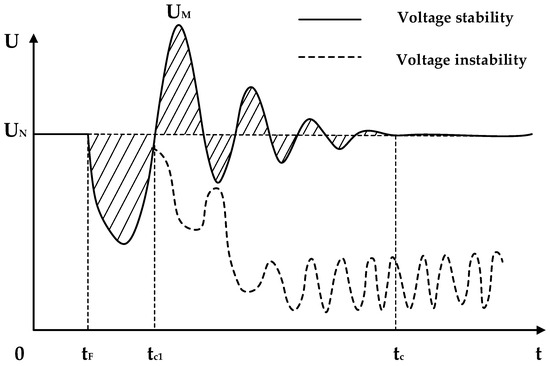
Figure 2.
Transient voltage response curve after disturbance.
After the fault is cleared, achieving a voltage stable state indicates that the system possesses a strong reactive voltage support capability as it can adjust the voltage to return within the stable range. Conversely, voltage instability implies the insufficient reactive power and voltage support capability of the system, leading to loss of stability in voltage and synchronous operation.
In order to comprehensively reflect the severity of power grid faults following system faults and the recovery of transient voltage after power grid faults are cleared, a transient voltage stability index (TVSI) has been proposed. This index includes the transient voltage disturbance index (TVDI) and the transient voltage peak index (TVPI). The purpose of configuring dynamic reactive power compensation devices is to maximize system voltage recovery to its initial level after fault clearance and ensure a more stable recovery process. The definition of TVDI holds great significance in reducing oscillations within the system. Additionally, for high-permeability PV power grids, it is necessary to suppress voltage overshoot phenomena. The definition of TVPI plays a crucial role in mitigating transient overvoltage occurrences at nodes where PV units with insufficient high-voltage crossing ability are located, thereby preventing system collapse.
3.1. Global Transient Voltage Disturbance Index
The transient voltage disturbance index is defined as:
where Ut,i is the voltage of node i at time t after the failure. Ui0 is the initial operating voltage of node i. In this paper, it is set as tF time voltage. Fk is the fault type studied.
The term TVDIiFk represents the integral of the difference between the voltage at node i and the normal rated voltage after fault Fk occurs, which quantifies the deviation between transient voltage and normal operating voltage. To facilitate programming calculations in time domain simulations, this equation can be differentiated as follows:
where h is the simulation step size in time domain simulation. This paper takes 0.01 s.
The TVDIiFk solely represents the transient voltage stability of node i. To comprehensively depict the global transient voltage stability of the power grid and investigate the overall weak areas in terms of voltage within the system, we define the global transient voltage disturbance index as follows:
The global transient voltage disturbance index is dependent on the maximum value of the system’s TVDI index, as demonstrated in Equation (13). Therefore, a smaller value of the transient voltage recovery index TVDI after fault clearance would result in a more advantageous restoration of the system’s transient stability.
3.2. Global Transient Voltage Peak Indicator
The transient voltage peak index (TVPI) is defined by Equation (14).
where TVPIiFk represents the severity of overvoltage of node i where the PV power station is located after Fk failure occurs. In order to give the severity of transient overvoltage of the nodes where all PV power stations are located in the system, the global peak transient voltage index is defined, as shown in Equation (15):
The global peak transient voltage indicator is determined by the node where the PV power station with the most severe transient overvoltage is located. The TVPIs index can be measured based on the voltage overshoot at a specific node. A smaller TVPI indicates a stronger voltage support capacity at the location of the PV power station, making it more challenging to disconnect the PV unit from the network.
4. Transient Reactive Power Planning Location Method
4.1. Typical Severe Fault
The magnitude of the fault hazard is related to the possibility of the fault and the severity of its consequences. Before site selection, the most serious typical faults that threaten the stable and safe operation of the power grid should be selected in different candidate scenarios, and the output probability and output size of the nodes equipped with PV should be calculated in the shutdown scenario, underpower scenario, and full power scenario.
The system should undergo N − 1 fault scanning in various scenarios, followed by the calculation of the TVDI and TVPI for different faults. Finally, the severity of each fault can be determined under different scenarios using Equation (16).
The fault severity in scenario i, denoted as ηi, is defined. PPV.i represents the output probability of the PV power station in three different scenarios: shutdown scenario (i = 1), underpower scenario (i = 2), and full power scenario (i = 3). The faults with the maximum ηi value in each scenario are considered as typical serious faults studied.
4.2. Filtering the Candidate Busbar Set to Be Compensated
The configuration process of the dynamic reactive power compensation device requires a careful analysis of the system’s buses to select suitable candidate buses and capacities. However, directly conducting capacity optimization for non-final buses in the simulation would double the simulation time and impact solving efficiency. Therefore, it is essential to determine the location step, i.e., the configuration of candidate buses, as a priority.
The location selection method takes into account both the static and dynamic characteristics of the power grid in this paper. By utilizing the comprehensive complex network theory’s static characteristic index and considering the interrelated topological structure within the system, a comprehensive understanding of the overall dynamic behavior characteristics is revealed. The nodes in the network are then sorted from largest to smallest based on this index, selecting the first N1 nodes as primary screening candidates for dynamic reactive power device compensation positions. This approach significantly reduces the available positions and node count, avoiding high-dimensional candidate node selection. Furthermore, by utilizing sensitivity theory’s dynamic characteristic index, it allows for further refinement of global transient voltage stability improvement when configuring different capacity dynamic reactive power compensation devices at various nodes.
The two site selection methods are related, but they have different emphases. This paper aims to fully utilize the advantages of both the static and dynamic characteristics of the power grid, and to select the optimal candidate installation node set from various perspectives to maintain transient voltage stability in the system.
4.2.1. Static Indicators Based on Complex Network Characteristics
The betweenness centrality and the closeness centrality are chosen in this paper to capture the static characteristics of network nodes [31].
- The betweenness centrality refers to the ratio of the number of shortest paths passing through a node to the sum of all shortest paths in the network. Typically, the weight assigned to each edge in the complex network is based on its corresponding admittance value in actual power lines. A higher admittance value indicates that power flow passes through this particular point more frequently in real networks. Consequently, a larger value for this index suggests that this point has potential to become a system hub. By configuring dynamic reactive power compensation devices at such points, capacitive reactive power can be efficiently distributed throughout the entire power grid and transient voltage fluctuations can be effectively controlled. The betweenness centrality of node i is:where nst(i) is the number of shortest paths passing through node s to node t and through node i at the same time. nst is the number of shortest paths from node s to node t.
- The closeness centrality represents the average shortest path between a given node and other nodes in a complex network. Typically, the impedance value of the actual line is utilized as the weight for the corresponding edge in the complex network. A higher value indicates a greater distance, implying that less power flows through this particular point in the actual network. This index provides an analysis from a positional perspective, allowing for an assessment of distances between nodes within the system and their proximity to central areas of the network. In practical power networks, being closer to these central areas warrants increased attention towards global transient voltage stability. The closeness centrality of node i can be expressed as:where vi is the number of nodes that node i can connect to (excluding i). N indicates the number of nodes in the network. Ci is the sum of the distance weights from node i to all connectable nodes, and the magnitude is the standardized impedance of its corresponding transmission line. If there is no path between node i and a node, c(i) is 0.
- The betweenness centrality and closeness centrality of nodes are normalized separately in order to comprehensively consider them, as demonstrated by Equations (19) and (20).where and are, respectively, the standard values of the betweenness centrality and the closeness centrality normalized for node i. bmin is the minimum value of intermediate centrality. bmax is the maximum value of intermediate centrality. cmin is the minimum value close to centrality. cmax is the maximum value close to centrality.The comprehensive index value ai of node i’s complex network characteristics can be obtained through the weighted summation of and , as demonstrated in Equation (21).where ai represents the comprehensive index value of complex network characteristics of node i. w1 and w2 represent weight coefficients. The sum of w1 and w2 is 1.
4.2.2. Dynamic Characteristic Index Based on Sensitivity Theory
The present study proposes a compensation sensitivity index (SI) that quantifies the relationship between the transient voltage stability index and the dynamic reactive power compensation amount, as depicted in Equation (22).
The compensation capacity of the installed dynamic reactive power device, denoted as ΔQC, determines the effectiveness of compensating for reactive power at a specific location. Equation (22) is used to conduct time domain simulations after a fault occurs in the research area. It is important to prioritize locations with higher compensation sensitivity values when planning for reactive power.
4.2.3. Differential Dynamic Reactive Power Compensation
The paper employs differential dynamic reactive power compensation for nodes with varying SI values, wherein distinct reactive power compensation devices are installed for each candidate node. Specifically, two types of dynamic reactive power compensation devices, namely the SVC and STATCOM, are utilized in this study.
Compared to the SVC, the STATCOM can provide a higher capacitive reactive power or absorb more capacitive reactive power in order to maintain transient voltage stability during significant drops or surges. In other words, STATCOM compensation is superior. Additionally, the STATCOM offers notable advantages over the SVC such as lower losses, faster response time, and reduced harmonic content. However, it should be noted that STATCOM control is complex and expensive. Taking all these factors into consideration, the STATCOM is preferred for the bus with the highest SI ranking among the candidate nodes while the SVC is utilized for the bus with the lowest SI ranking. The objective is to rapidly increase reactive power during initial failure stages to ensure system voltage stability and maximize cost savings [32].
4.3. Transient Reactive Power Capacity Planning Model
4.3.1. Objective Function
One of the optimization objectives of the reactive power capacity planning model is to enhance transient voltage stability, improve post-failure transient voltage recovery capability, and mitigate transient overvoltage. The second objective is to minimize the cost of dynamic reactive power compensation devices while ensuring transient voltage stability. Therefore, the objective function of the proposed reactive power capacity planning model in this paper is represented by Equations (23) and (24).
where TVDIs is the global transient voltage disturbance index. TVPIs is the global peak value of transient voltage. TSVC and TSTATCOM are the service life of the SVC and the STATCOM in the system, respectively. NSVC and NSTATCOM are the total number of SVCs and STATCOMs in the system, respectively. CSVC and CSTATCOM are the unit price of reactive power compensation of the SVC and STATCOM, respectively. QSVC and QSTATCOM are the reactive power compensation capacities of the SVC and STATCOM in the system, respectively. FSVC and FSTATCOM are the installation costs of the SVC and STATCOM, respectively.
F1 represents the transient voltage stability, which refers to the phenomenon where a PV power station enters a low-pass state after a fault and generates excessive reactive current that persists even after the fault is cleared. This surplus of reactive power leads to transient overvoltage, posing significant threats to the normal and safe operation of the system. Therefore, it is crucial to consider the peak value of transient voltage in the objective function. Additionally, Figure 2 demonstrates that severe disturbances in the system can result in extreme voltage instability and collapse, thereby jeopardizing system security. In such cases, addressing extreme voltage instability solely based on peak values of transient voltage becomes insufficient. Hence introducing a measure for assessing transient voltage disturbance index becomes highly necessary. F2 represents the economic aspect of dynamic reactive power compensation devices by taking into account both their unit price and installation cost.
4.3.2. Constraint Condition
- Equality constraintThe equality constraint represents the power flow restriction in the system.where the variables PG.i, QG.i, PL.i, and QL.i represent the injected active power, injected reactive power, active load, and reactive load of generator node i, respectively. Ui, Uj, θi, and θj denote the voltage amplitude of node i, the voltage amplitude of node j, the voltage phase angle of node i and the voltage phase angle of node j, respectively. Gij and Bij correspond to the conductance and susceptance values for line i-j.
- Inequality constraintThe range of state variables and control variables in the inequality constraints:where PPV,q is the active power output of the q PV power station. PPV,q.max, PPV,q.min are the upper and lower limits, respectively. QPV,q is the reactive power output of the q PV power station. QPV,q.max, QPV,q.min are the upper and lower limits, respectively. QSVC,g is the reactive power output of the SVC station g. QSVC, g.max, QSVC, g.min are the upper and lower limits, respectively. QSTATCOM,h is the reactive power output of the h STATCOM. QSTATCOM,h.max, QSTATCOM,h.min are the upper and lower limits, respectively. Pgk is the active power output of the k generator. Pgk,max, Pgk,min are the upper and lower limits, respectively. Qgk is the reactive power output of the k generator. Qgk,max, Qgk,min are the upper and lower limits, respectively. Ui is the voltage amplitude of the i node. Ui,max, Ui,min are the upper and lower limits, respectively. NPV, NSVC, NSTATCOM, NG, and N are, respectively the total number of PV power stations, total number of SVCs, total number of STATCOMs, total number of generators, and total number of nodes in the system.
4.4. Model Solving
4.4.1. MOMPA
The multi objective marine predator algorithm (MOMPA) is an optimization algorithm that leverages the predator-hunting rule of marine predators, offering distinct advantages in terms of precision and accuracy.
Compared with widely used particle swarm algorithm, genetic algorithm, cuckoo search algorithm, and Salpa algorithm developed in recent years, the marine predator algorithm has shown superior computational efficiency and convergence performance, which has been effectively verified in the literature [33]. In the algorithm, vortex formation or fish aggregating devices (FADs) and marine memory updates are introduced. The former takes into account the impact of an ocean vortex and artificial fish gathering device on the population in a real scene and reduces the possibility of the population falling into a local optimal through a secondary population update. The latter helps the predator remember the location of the prey-rich area where it successfully foraged before, compared to the equivalent term in the previous iteration.
In MOMPA, the ocean represents the feasible domain of the optimization problem, the elite predator matrix E represents the global optimal solution, and the prey matrix P represents the current optimal solution. Based on the predation relationship between marine predators and prey, the MOMPA iteration process is divided into the four parts specified below.
- Population initialization: MOMPA is a population-based optimization method, which can be randomly generated to initialize the population and obtain the initial elite matrix E and prey matrix P, which represent the global optimal solution and the current optimal solution, respectively. The marine predator algorithm constructs the initial prey matrix P0 according to the population number N and individual dimension d, selects the prey individual with the best fitness as the top predator E, and initializes the marine environment using Formula (26):where Pmax indicates the upper bound; Pmin indicates the lower bound; rand(0, 1) is used as a uniformly distributed random number [0, 1], essentially a uniform random vector in the range of (0, 1).
- Iteration of population optimization: It includes three iteration stages: high-speed ratio stage, equal-velocity ratio stage, and low-velocity ratio stage to update the moving step size and position of the population.Early iteration of population: When the prey are moving faster than the predators, that is, in the high-rate ratio phase. The optimal strategy for predators is not to move, in which case the population action can be expressed as:where v is the number of current iterations; vmax is the maximum number of iterations; i = 1,……, N, N is the population number; si is the moving step vector; RB is a random vector of Brownian motion; ⊗ is the Kronecker product; Ei is the i row vector of elite matrix; Pi is the row i vector of the prey matrix. c1 = 0.5, is a constant term; R is a random number vector between [0, 1].Middle phase of population iteration: When the prey and the predator move at similar speeds, that is, in the phase of equal rate ratio. The population is divided into two parts: detection and exploitation to further find the optimal solution.For the first half of the population i = 1, …, N/2, detected by Levi motion, can be written as:where RL is a random vector of Levi motion.For the latter half of the population i = N/2, …, N, developed by Brownian motion, can be written as:where c2 is an adaptive parameter controlling the predator’s moving step length.End of population iteration: When the predator is moving faster than the prey, that is, it is in the low-rate ratio phase. Predators perform Levi movements to improve local search capabilities, which can be written as:
- Eddy currents and artificial fish aggregating devices (FADs): It is related to environmental topics such as the effects of fish collecting devices or eddy formation. These conditions affect the behavior of marine predators. Therefore, according to the above situation, the following mathematical formula is proposed.where cFAD represents the effect coefficient of eddy current and artificial fish aggregating device, usually cFAD = 0.2; Xmax and Xmin are the upper and lower boundary line vectors of the optimization variables, respectively; U is a randomly generated binary row vector [0, 1]; r is the random number between [0, 1]; r1 and r2 represent the random index of the prey matrix.
- Marine memory Update: This step is related to the ability to remind predators of the best places to forage successfully. This capability saves memory in MOMPA. This is done iteratively to improve the quality of the solution. After the solution is updated, the current solution is compared to the historical solution, and if the historical solution is better than the current solution, the current solution will be replaced by the historical solution.
4.4.2. Software Call Relation
The model is solved using Matlab and PSAT 2.1.11. Firstly, a multi-objective optimization algorithm is implemented in Matlab, with the algorithm parameters set accordingly. Then, the PSAT simulation software is invoked to pass the optimization control variables to PSAT. Specifically, this involves modifying the capacity parameters of the SVC and STATCOM in the time domain simulation variables of PSAT. A simulated example system is constructed on the PSAT platform, where fault parameters are defined and a time domain simulation is executed. The resulting data from the time domain simulation, such as voltage changes at each node, susceptance changes of SVC, and the reactive current changes of the STATCOM, are returned to Matlab for analysis. This process iterates until reaching the maximum number of iterations T_Max as specified. The specific invocation relationship can be seen in Figure 3.
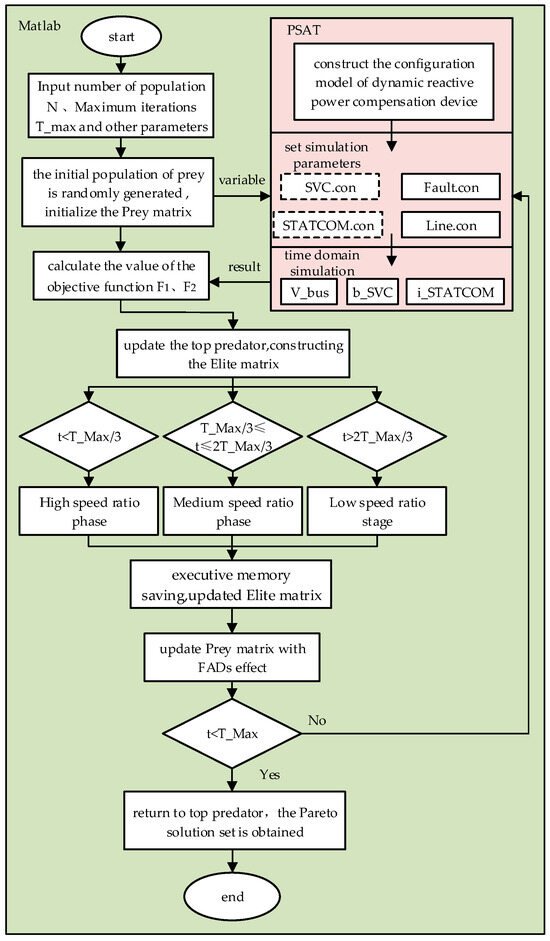
Figure 3.
The calling relationship between the MOMPA and PSAT in Matlab.
4.4.3. Multi-Criteria Decision Making Method
After the above multi-objective algorithm optimization steps are completed, a set of non-dominated solutions will be obtained, and the corresponding Pareto solution set will be obtained, and the corresponding scheme selection will be made according to the non-dominated solutions. This method is multi-criteria decision making. Multi-criteria decision-making can help analyze the influence of different criteria on the final scheme and make the most appropriate decision based on the importance of each criterion.
In this paper, an improved TOPSIS evaluation method is used to select the optimal configuration scheme of the dynamic reactive power compensation device from a set of non-dominated solutions. The traditional TOPSIS evaluation method based on the entropy weight method only uses the entropy weight method to assign weights to each index, and the uncertainty is large. The improved TOPSIS evaluation method uses the entropy weight method and the standard deviation method to comprehensively assign weights, which makes the evaluation results more accurate. The specific steps are as follows [34]:
- Unify the types of indicators, including very small indicators, intermediate indicators, interval indicators and very large indicators. Let there be a total of n schemes with m indicators and let the j index value of the i scheme be xij. First, all indicators are converted into extremely large indicators, and both indicators in this paper are extremely small indicators.
- Form a positive matrix and standardize the matrix to eliminate the influence of different dimensions. Let zij be the j index value of the i scheme normalized by the forward matrix.
- The entropy weight method and the standard deviation method are used to comprehensively assign weights to different indicators. Both the entropy weight method and the standard deviation method belong to the objective weighting method. The principle of the entropy weight method is that the smaller the degree of dispersion of the index data, the less information it reflects, and the lower the corresponding weight value. The standard deviation method assigns weights to each evaluation index according to the variation degree between the current value and the target value. The core is to assign weights by the ratio between the standard deviation value reflecting the dispersion degree of each index and the mean value of each index. The weighting formula is as follows:where Wj is the comprehensive weight of the evaluation index; W1j is the weight of the evaluation index obtained by using entropy weight method; W2j is the weight of the evaluation index obtained using the standard deviation method.
- Calculate the score values for different schemes.where Zj+ and Zj− are, respectively the maximum and minimum values of all schemes under the j index; Di+ and Di− are the distance between the i scheme value and the maximum and minimum values, respectively; Si is the final score of scheme i.
4.4.4. Configuration Procedure of the Dynamic Reactive Power Compensation Device
The specific configuration steps of the dynamic reactive power compensation device are shown in Figure 4.
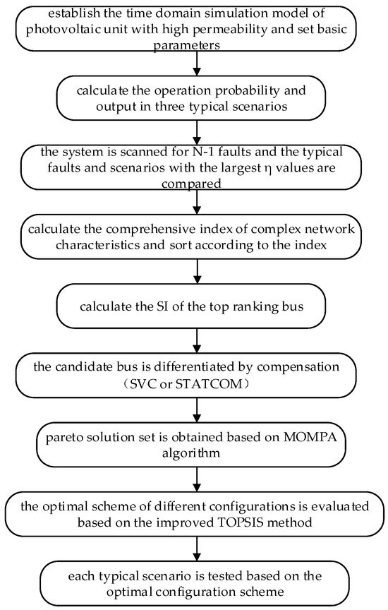
Figure 4.
Configuration procedure of the dynamic reactive power compensation device.
- Calculate the operational probability and output of the PV unit in scenarios such as the shutdown scenario, underpower scenario, and full power scenario.
- Conduct an N − 1 fault scan for the system to determine the baseline scenario for dynamic reactive power planning and identify typical severe faults.
- Select static indicators of the system network bus based on complex network characteristics, calculate comprehensive indicators for each bus’s complex network characteristics, and sort them to select the top candidate bus set.
- Calculate and select the SI value of each candidate bus to complete final screening and obtain a bus set with optimal compensation effect.
- Prepare for installing the STATCOM on the top bus within the candidate bus set, prepare for installing the SVC on the bottom bus, and construct different configuration schemes with various compensation devices.
- Utilize the MOMPA algorithm along with time domain simulation results from different configuration schemes to solve Pareto solution sets.
- Apply the improved TOPSIS method to evaluate each configuration scheme, calculate the score values for each scheme, and select the scheme with highest score as the optimal configuration scheme.
- The time-domain simulation verification of the shutdown scenario, underpower scenario, and full power scenario is re-executed based on the optimal configuration scheme.
5. Example Analysis
5.1. Example Setting and Solving
5.1.1. Example Setting
In this paper, time domain simulation and optimization operations are conducted on an improved IEEE39-node system using MATLAB and its PSAT toolbox for power system analysis and control. The proposed dynamic reactive device configuration method is the main focus of this study. The detailed parameters of the branch, generator, and other components are referenced from [35], while the load consists of 50% induction motor load and 50% constant impedance load. Figure 5 shows the wiring diagram of the improved IEEE39-node system.
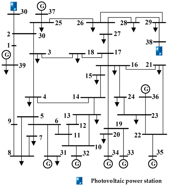
Figure 5.
Improved IEEE39-node system.
The PV power station is connected to the grid via buses 30 and 38, and based on Equation (38), the PV penetration in the enhanced IEEE39-node system reaches 20.3%, satisfying high-penetration requirements.
where ρ% is the permeability of PV power generation in the grid. PPV.r is the installed capacity of the r PV power station in the power grid; q is the total number of PV power stations in the grid. PL.sum is the total active power of all generators in the grid.
The key parameters utilized by the PV cells in the PV power stations are presented in Table 1.

Table 1.
Main parameters of the PV cells.
According to Formulas (1)–(10), the probability and output of PV units in PV systems with high permeability can be obtained under various scenarios, as illustrated in Table 2.
Table 2.
Improved typical PV scenario parameters in IEEE 39-node system.
5.1.2. Solving Typical Serious Faults
According to the analysis in Section 4.1, for subsequent analysis, it is recommended to select the scenario with the highest ηi value among the three typical scenarios with different PV output. A higher ηi value indicates a greater likelihood of transient voltage instability in the system. Within the same scenario, different faults on different nodes correspond to varying ηi values. After running normally for 1 s in all three typical scenarios, single-phase ground fault and three-phase short-circuit fault were introduced separately at different bus bars for a duration of 0.1 s each. The resulting data is presented in Table 3. In scenario PV.2, when a three-phase short circuit occurs at node 16, it yields the highest η value and Figure 6 illustrates the voltage waveform across all network buses during this fault. In the following figure about the voltage waveform, the colored lines are the voltage waveform of each point of the 39 nodes, and the shaded part is the area of continuous operation of the photovoltaic power station without off-grid. Due to space limitations, the legend does not show all of them.
Table 3.
Transient instability of bus voltage in the whole network under different scenarios.
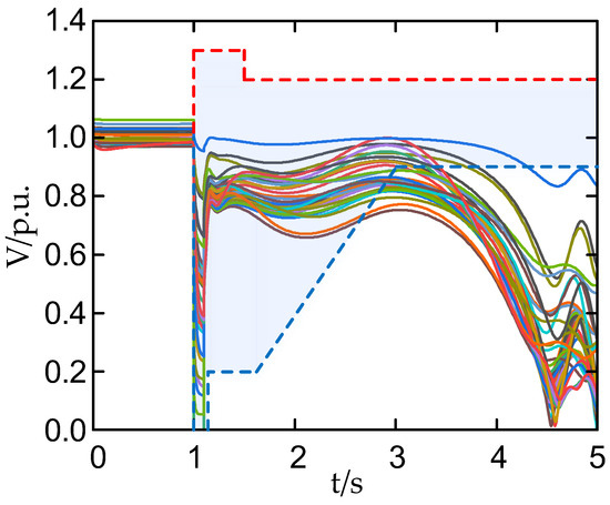
Figure 6.
Buses’ voltage waveform of the whole network after a 16-node three-phase short-circuit fault in the PV.2 scenario.
5.1.3. The Candidate Busbar Set to Be Compensated Is Solved
- First, the IEEE39-node system is represented as a complex network diagram wherein each line is depicted by edges and each bus is denoted by nodes. The resulting complex network diagram, illustrated in Figure 7, showcases the composition of 39 nodes and 46 edges.
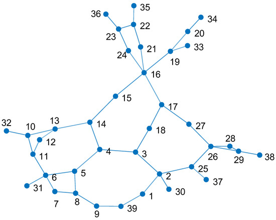 Figure 7. IEEE39 node system complex network diagram.The betweenness centrality and closeness centrality of each node in Figure 7 were computed, as presented in Table 4. To preliminarily identify potential node schemes for PV power stations, both the betweenness centrality and closeness centrality are considered to have equal influence. Therefore, w1 and w2 are assigned values of 0.5 each to calculate the comprehensive index of complex network characteristics for each node, as depicted in Figure 8.
Table 4. The betweenness centrality and the closeness centrality of each node.
Figure 7. IEEE39 node system complex network diagram.The betweenness centrality and closeness centrality of each node in Figure 7 were computed, as presented in Table 4. To preliminarily identify potential node schemes for PV power stations, both the betweenness centrality and closeness centrality are considered to have equal influence. Therefore, w1 and w2 are assigned values of 0.5 each to calculate the comprehensive index of complex network characteristics for each node, as depicted in Figure 8.
Table 4. The betweenness centrality and the closeness centrality of each node.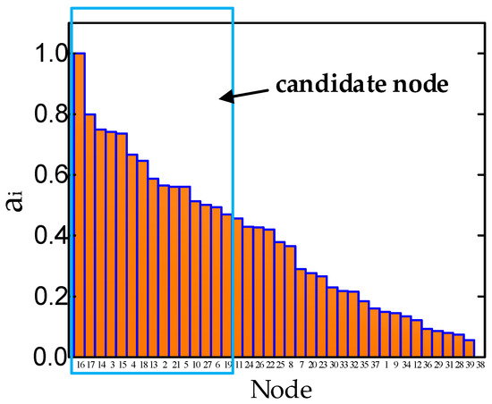 Figure 8. Comprehensive index value of complex network characteristics of all nodes.The final screening process involves selecting the top 15 points from Figure 8’s comprehensive index of complex network characteristics.
 - Generally, the installation of dynamic reactive power compensation devices is not recommended on buses where synchronous generators are located, considering a constant voltage amplitude. Figure 8 illustrates that the bus ranking for these locations is lower. To specifically assess the impact of installing dynamic reactive power compensation devices with identical capacity on TVDIs and TVPIs at different nodes, a 100 Mvar STATCOM is connected to each candidate node mentioned above. The sensitivity index (SI) for each node is then calculated using Equation (22). The calculation results are presented in Figure 9.
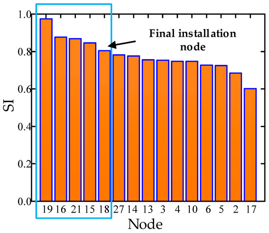 Figure 9. Some node sensitivity indicators.The installation of STATCOM with the same capacity on different nodes results in varying degrees of reduction in TVDIs and TVPIs, as depicted in Figure 9. Notably, deploying STATCOM on specific nodes yields significant reductions in both TVDIs and TVPIs.Considering the high construction cost associated with having more than six reactive power compensation sites, and the adverse effects of a small compensation location (less than four stations) resulting in increased network loss and worsened transient compensation effect due to excessive reactive power transmission, five optimal reactive power compensation stations are selected: bus 19, 16, 21, 15, and 18. Furthermore, it should be noted that the research method proposed in this paper is applicable to all candidate busbars without repetition.
5.1.4. Differential Compensation
In order to directly reflect the disparity in compensation performance between the STATCOM and the SVC during fault occurrences, an example is taken from the system described in this paper. A STATCOM and SVC with identical capacities of 400 Mvar are installed at bus bar 19, respectively. The reactive power response characteristics of the corresponding reactive power compensation devices and the voltage changes at bus bar 16 nodes are observed, as depicted in Figure 10.
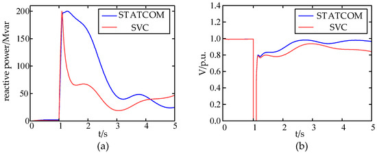
Figure 10.
Comparison of compensation performance between the STATCOM and the SVC. (a) Reactive response when the STATCOM and the SVC are compensated, and (b) bus voltage when the STATCOM and the SVC are compensated.
It is evident that both the STATCOM and the SVC possess the capability to swiftly generate a substantial amount of reactive power in the event of a system failure, thereby supporting fault bus voltage, mitigating transient voltage instability, and expediting the restoration of normal operation. Moreover, it is apparent that the STATCOM outperforms the SVC in terms of reactive power compensation effectiveness, output stability, and overall compensation performance [35].
The economic parameters and investment costs of dynamic reactive power compensation devices are shown in Table 5. For the first 5 busbars selected, STATCOM is used to compensate those with high sensitivity, focusing on the overall reactive power compensation effect. With low sensitivity, SVC is used for compensation, focusing on economic considerations, that is, to maximize economic benefits on the basis of meeting the demand for reactive power compensation.
Table 5.
Economic parameters and investment cost of dynamic reactive power compensation device.
5.1.5. Example Solving
After determining the candidate nodes for typical serious faults and dynamic reactive power compensation devices, the MOMPA algorithm is applied based on the configuration method process of reactive power compensation devices outlined in Section 4.4.4. The population size is set to 20, with a maximum of 60 iterations allowed. The capacity limits for each candidate busbar installation are defined as an upper limit of 500 Mvar and a lower limit of 0 Mvar. Figure 11 illustrates the Pareto frontier solution set results obtained from different solutions using the MOMPA algorithm.
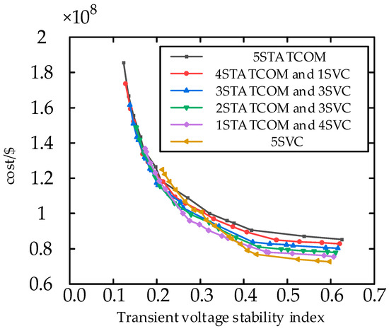
Figure 11.
The configuration results of each optimal scheme.
The increase in dynamic reactive power compensation cost leads to a better effect on maintaining the transient voltage stability of the system as each device compensates for more reactive power, indicating a positive correlation between the two factors. There exists a certain saturation point between the compensated transient voltage stability index and the configured capacity, where an increase in capacity beyond this point results in diminishing reduction effects of the compensation device on the index while exponentially increasing costs. Hence, it is essential to evaluate the relationship between compensation effect and cost for each scheme using an improved entropy weight TOPSIS method to select the optimal configuration scheme.
The evaluation results and rankings of each program are presented in Table 6, while Table 7 displays the bus capacity configurations for different schemes. As indicated by Table 6, Scheme 3 exhibits superior reactive power compensation effectiveness with a lower economic cost compared to Scheme 1. Scheme 2 demonstrates the lowest economic cost and better reactive power compensation effect than Scheme 6. In conclusion, when compared to compensation schemes solely adopting an SVC or a STATCOM, the improved entropy weight TOPSIS method generally yields higher scores in evaluation. These schemes not only enhance transient voltage stability at fault buses and key buses but also consider the economic aspect of compensation comprehensively. Therefore, Scheme 3 is selected as the final configuration in this study. The voltage waveforms of all buses throughout the network after implementing this scheme are illustrated in Figure 12.
Table 6.
Evaluation results of different optimal compensation schemes.
Table 7.
Optimal configuration scheme of dynamic reactive power compensation device.
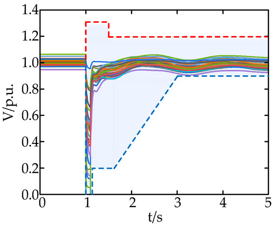
Figure 12.
The buses’ voltage waveform has been configured in the PV.2 scenario.
5.2. Analysis and Verification of Simulation Results
5.2.1. Multi-Scene Simulation and Comparison
The validity of the proposed configuration method is examined through the investigation of three different configuration schemes in this paper.
Scheme 1: Scheme 1 focuses solely on the location planning of dynamic reactive power compensation devices, without considering capacity optimization. Specifically, 186.6 Mvar dynamic reactive power compensation devices are allocated to nodes 19, 16, 21, 15 and 18, while maintaining the same reactive power source control voltage as Scheme 3.
Scheme 2: Reactive power capacity optimization is exclusively considered in Scheme 2. The configuration of reactive power capacity is focused on the five nodes with the lowest sensitivity, namely nodes 10, 6, 5, 2 and 17, as illustrated in Figure 9.
Scheme 3: The adopted scheme is Scheme 3, which comprehensively considers the location planning and reactive power capacity planning of the dynamic reactive power compensation device. This scheme refers to the optimal configuration method proposed in this paper for the dynamic reactive power compensation device.
The comparison of Pareto solution sets between Scheme 2 and Scheme 3 is illustrated in Figure 13. Table 8 presents the capacity configurations for each solution. The results of the three configuration schemes are displayed in Table 9. It can be observed from Table 9 that, in Scheme 1’s configuration, the TVDI experiences an impressive reduction of 85.61%, while the transient voltage stability index decreases by a significant margin of 84.94% compared to its pre-configuration state. In Scheme 2’s configuration, the TVDI exhibits a substantial decrease of 76.51%, accompanied by a notable decline of the transient voltage stability index by approximately74.41%. Lastly, Scheme 3’s configuration leads to a remarkable decrease in the TVDI by as much as 86.32%, along with an equally noteworthy reduction in the transient voltage stability index amounting to 85.73%.
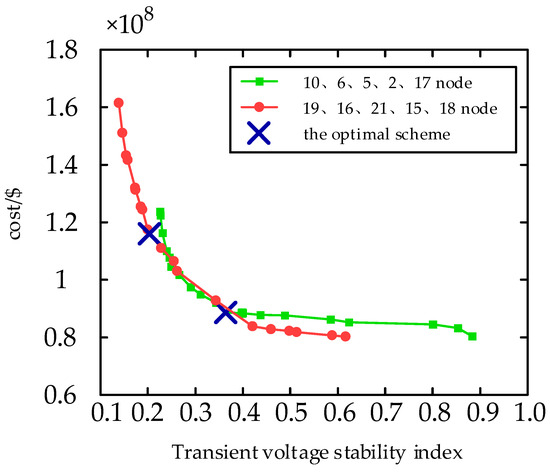
Figure 13.
Configuration results of Solution 2 and Solution 3.
Table 8.
Optimal configuration scheme of three kinds of dynamic reactive power compensation devices.
Table 9.
Comparison of the three configuration schemes.
The proposed dynamic reactive power compensation scheme, Scheme 3, is employed for configuration. Simulation results demonstrate that compared to Scheme 1, the transient voltage stability index experiences a reduction of 5.23% under constant configuration cost conditions. Furthermore, in comparison to Scheme 2, the transient voltage stability index is reduced by 44.23%, albeit with an increase in configuration cost of 30.79%.
The compensation effect of Scheme 3 is observed to be the most optimal, and in comparison with Scheme 2, the configuration obtained through the location scheme proposed in this paper demonstrates superior ability to maintain system transient stability following failure. Moreover, at an equivalent cost, the solution derived from the multi-objective optimization algorithm proves more effective than its counterpart in enhancing transient stability.
5.2.2. Configuration Scheme Verification
The optimal configuration scheme obtained in the previous section is utilized to verify scenario PV.1 and scenario PV.3. Figure 14 and Figure 15 illustrate the voltage waveforms of each bus in the entire network before and after the configuration, while Table 10 presents the specific results.
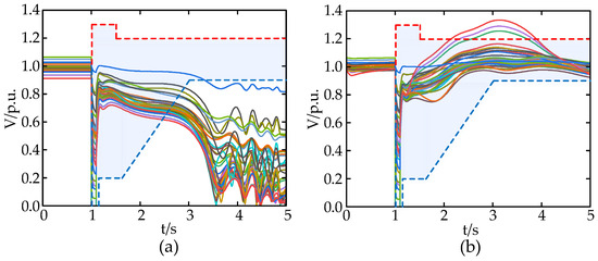
Figure 14.
The buses’ voltage waveform of the whole network after the fault (a) in the PV.1 scenario and (b) in the PV.3 scenario.
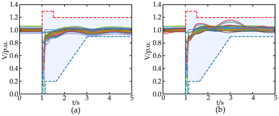
Figure 15.
The buses’ voltage waveform has been configured in the (a) PV.1 scenario and (b) PV.3 scenario.
Table 10.
Comparison of the results of the optimal configuration scheme in scenario PV.1 and scenario PV.3.
The results in Table 10 demonstrate that in scenario PV.1, following the configuration, the TVDI index experiences a significant decrease of 92.34%, while the TVPI index exhibits an increase of 18.96%. Additionally, the transient voltage stability index shows a substantial reduction of 90.9% compared to its pre-configuration value. In scenario PV.3, after the configuration, there is a reduction of 47.37%, 12.99%, and 54.21% observed in the TVDI indicator, the TVPI indicator, and the transient voltage stability indicator, respectively, when compared to their respective values before the configuration.
The optimal scheme obtained has been proven to effectively address the transient voltage stability problem caused by voltage instability, enhance the system’s voltage support capability, mitigate transient overvoltage issues, and prevent off-grid situations for PV units due to insufficient high voltage crossing capability.
6. Conclusions
The paper proposes a dynamic reactive power compensation device configuration method that takes into account the overall transient voltage stability of a PV system with high permeability.
The uncertainty of PV unit output is prioritized in the configuration of reactive power compensation to ensure the suitability of the method for diverse unit output conditions.
When planning site selection in this paper, the complex network characteristics of nodes within a complex network system are initially considered as the benchmark, followed by assessing the sensitivity of different nodes. This enables the rapid identification of critical nodes within the system and reduces the scale of simulation optimization.
The transient voltage stability index, which takes into account the indices of transient voltage disturbance and transient voltage peak, can effectively quantify the transient voltage stability of each bus in the system and provide guidance for configuring dynamic reactive power compensation equipment.
The differentiated reactive power compensation method employed in this paper offers a novel concept and foundation for the practical configuration of reactive power compensation device engineering. It not only ensures transient voltage stability at the global bus, but also significantly reduces procurement costs.
The integration of static voltage stability and transient voltage stability is the primary research focus in configuring dynamic reactive power devices.
Author Contributions
The authors confirm their contributions as follows: Y.L. and D.Y. proposed the innovations and wrote the paper; methodology, Y.G.; software, J.L.; C.L. and D.G. reviewed the simulation results and revised the manuscript. All authors have read and agreed to the published version of the manuscript.
Funding
This research was funded by National Key Research and Development Program of China, grant number 2019YFB1505400.
Data Availability Statement
Data is contained within the article.
Conflicts of Interest
The authors declare no conflict of interest.
References
- Trieu, M.; Maureen, H.M.; Samuel, F.B.; Ryan, H.W.; Greg, L.B.; Paul, D.; Doug, J.A.; Gian, P.; Debra, S.; Donna, J.H.; et al. Renewable Electricity Futures for the United States. IEEE Trans. Sustain. Energy 2014, 5, 372–378. [Google Scholar]
- Guangul, F.M.; Chala, G.T. Solar Energy as Renewable Energy Source: SWOT Analysis. In Proceedings of the 2019 4th MEC International Conference on Big Data and Smart City (ICBDSC), Muscat, Oman, 15–16 January 2019; pp. 1–5. [Google Scholar]
- Mukherjee, A.; Roy, N.; Kumar, A.; Prakash, C.; Sanskriti, S.; Rout, N.K. Maximum Utilisation of Solar Energy for Smart Home Lighting System. In Proceedings of the 2018 International Conference on Recent Innovations in Electrical, Electronics & Communication Engineering (ICRIEECE), Bhubaneswar, India, 27–28 July 2018; pp. 3286–3290. [Google Scholar]
- Rivera, M.; Rojas, D.; Fuentes, R.; Wheeler, P. Development of Solar Energy in Chile and the World. In Proceedings of the 2021 IEEE 48th Photovoltaic Specialists Conference (PVSC), Fort Lauderdale, FL, USA, 20–25 June 2021; pp. 2453–2457. [Google Scholar]
- Kawabe, K.; Tanaka, K. Impact of Dynamic Behavior of Photovoltaic Power Generation Systems on Short-Term Voltage Stability. IEEE Trans. Power Syst. 2015, 30, 3416–3424. [Google Scholar] [CrossRef]
- Yu, J.; He, T.; Wu, J.; Xu, J.; Wang, D.; Yu, Y. Study on Small Disturbance Stability of Photovoltaic Grid-Connected Power Generation System. In Proceedings of the 2023 5th Asia Energy and Electrical Engineering Symposium (AEEES), Chengdu, China, 23–26 March 2023; pp. 1429–1433. [Google Scholar]
- Ni, Q.; Zhu, X.; Hao, W.; Wang, X.; Zhou, Z.; Gan, D. A Voltage Stability Study for Power Systems Integrated with Photovoltaics. In Proceedings of the 2023 9th International Conference on Electrical Engineering, Control and Robotics (EECR), Wuhan, China, 24–26 February 2023; pp. 192–196. [Google Scholar]
- Sarbazi, J.; Najafabadi, A.A.; Hosseinian, S.H.; Gharehpetian, G.B.; Khorsandi, A. Effects of Photovoltaic Power Plants Grid Code Requirements on Transient Stability. In Proceedings of the 2022 12th Smart Grid Conference (SGC), Kerman, Iran, 13–15 December 2022; pp. 1–7. [Google Scholar]
- Montoya, O.D.; Fuentes, J.E.; Moya, F.D.; Barrios, J.Á.; Chamorro, H.R. Reduction of Annual Operational Costs in Power Systems through the Optimal Siting and Sizing of STATCOMs. Appl. Sci. 2021, 11, 4634. [Google Scholar] [CrossRef]
- Sapkota, B.; Vittal, V. Dynamic VAr Planning in a Large Power System Using Trajectory Sensitivities. IEEE Trans. Power Syst. 2010, 25, 461–469. [Google Scholar] [CrossRef]
- Tiwari, A.; Ajjarapu, V. Optimal Allocation of Dynamic VAR Support Using Mixed Integer Dynamic Optimization. IEEE Trans. Power Syst. 2011, 26, 305–314. [Google Scholar] [CrossRef]
- Wildenhues, S.; Rueda, J.L.; Erlich, I. Optimal Allocation and Sizing of Dynamic Var Sources Using Heuristic Optimization. IEEE Trans. Power Syst. 2015, 30, 2538–2546. [Google Scholar] [CrossRef]
- Van Cutsem, T. A method to compute reactive power margins with respect to voltage collapse. IEEE Trans. Power Syst. 1991, 6, 145–156. [Google Scholar] [CrossRef]
- Delfanti, M.; Granelli, G.P.; Marannino, P.; Montagna, M. Optimal capacitor placement using deterministic and genetic algorithms. IEEE Trans. Power Syst. 2000, 15, 1041–1046. [Google Scholar] [CrossRef]
- Lakkaraju, T.; Feliachi, A. Selection of Pilot buses for VAR Support Considering N-1 Contingency Criteria. In Proceedings of the 2006 IEEE PES Power Systems Conference and Exposition, Atlanta, GA, USA, 29 October–1 November 2006; pp. 1513–1517. [Google Scholar]
- Pourbeik, P.; Koessler, R.J.; Quaintance, W.; Wong, W. Performing Comprehensive Voltage Stability Studies for the Determination of Optimal Location, Size and Type of Reactive Compensation. In Proceedings of the 2006 IEEE PES Power Systems Conference and Exposition, Atlanta, GA, USA, 29 October–1 November 2006; p. 118. [Google Scholar]
- Huang, Y.-C.; Yang, H.-T.; Huang, C.-L. Solving the capacitor placement problem in a radial distribution system using Tabu Search approach. IEEE Trans. Power Syst. 1996, 11, 1868–1873. [Google Scholar] [CrossRef]
- Garrido-Arévalo, V.M.; Gil-González, W.; Montoya, O.D.; Chamorro, H.R.; Mírez, J. Efficient Allocation and Sizing the PV-STATCOMs in Electrical Distribution Grids Using Mixed-Integer Convex Approximation. Energies 2023, 16, 7147. [Google Scholar] [CrossRef]
- Nanibabu, S.; Shakila, B.; Prakash, M. Reactive Power Compensation using Shunt Compensation Technique in the Smart Distribution Grid. In Proceedings of the 2021 6th International Conference on Computing, Communication and Security (ICCCS), Las Vegas, NV, USA, 4–6 October 2021; pp. 1–6. [Google Scholar]
- Kumar, P.; Bohre, A.K. Optimal allocation of Hybrid Solar-PV with STATCOM based on Multi-objective Functions using combined OPF-PSO Method. SSRN Electron. J. 2021, 2021, 1–12. [Google Scholar] [CrossRef]
- Montoya, O.D.; Chamorro, H.R.; Alvarado-Barrios, L.; Gil-González, W.; Orozco-Henao, C. Genetic-Convex Model for Dynamic Reactive Power Compensation in Distribution Networks Using D-STATCOMs. Appl. Sci. 2021, 11, 3353. [Google Scholar] [CrossRef]
- Pourdaryaei, A.; Shahriari, A.; Mohammadi, M.; Aghamohammadi, M.R.; Karimi, M.; Kauhaniemi, K. A New Approach for Long-Term Stability Estimation Based on Voltage Profile Assessment for a Power Grid. Energies 2023, 16, 2508. [Google Scholar] [CrossRef]
- Lee, Y.; Song, H. A Reactive Power Compensation Strategy for Voltage Stability Challenges in the Korean Power System with Dynamic Loads. Sustainability 2019, 11, 326. [Google Scholar] [CrossRef]
- Zhu, Y.; Liao, W.; Nie, C.; Xie, W.; Xu, J.; Li, Y. The multi-objective optimal allocation method of static var compensator based on transient voltage security control. J. Phys. Conf. Ser. 2020, 1633, 012136. [Google Scholar] [CrossRef]
- Yang, D.; Cheng, H.; Ma, Z.; Sun, Q.C.; Yao, L.Z.; Zhu, Z.L. Integrated reactive power planning methodology considering static and transient voltage stability for AC-DC hybrid system. Proc. CSEE 2017, 37, 3078–3086+3363. [Google Scholar]
- Li, X.; Xu, M. Assessment of Transient Voltage Stability of Load Bus Considering Mechanical Torque of Dynamic Load. Autom. Electr. Power Syst. 2010, 34, 11–14+19. [Google Scholar]
- Xu, Y.; Dong, Z.Y.; Meng, K.; Yao, W.F.; Zhang, R.; Wong, K.P. Multi-Objective Dynamic VAR Planning Against Short-Term Voltage Instability Using a Decomposition-Based Evolutionary Algorithm. IEEE Trans. Power Syst. 2014, 29, 2813–2822. [Google Scholar] [CrossRef]
- Zhang, Y.; Zhou, Q.; Zhao, L.; Ma, Y.; Lv, Q.; Gao, P. Dynamic Reactive Power Configuration of High Penetration Renewable Energy Grid Based on Transient Stability Probability Assessment. In Proceedings of the 2020 IEEE 4th Conference on Energy Internet and Energy System Integration (EI2), Wuhan, China, 11–13 November 2020; pp. 3801–3805. [Google Scholar]
- Chao, L.; Yongting, C.; Xunjun, Z. Analysis and Solution of Voltage Overvoltage Problem in Grid Connection of Distributed Photovoltaic System. In Proceedings of the 2018 China International Conference on Electricity Distribution (CICED), Tianjin, China, 17–19 September 2018; pp. 1114–1117. [Google Scholar]
- Biswas, P.P.; Suganthan, P.N.; Amaratunga, G.A. Optimal power flow solutions incorporating stochastic wind and solar power. Energy Convers. Manag. 2017, 148, 1194–1207. [Google Scholar] [CrossRef]
- Saleh, M.; Esa, Y.; Onuorah, N.; Mohamed, A.A. Optimal microgrids placement in electric distribution systems using complex network framework. In Proceedings of the 2017 IEEE 6th International Conference on Renewable Energy Research and Applications (ICRERA), San Diego, CA, USA, 5–8 November 2017; pp. 1036–1040. [Google Scholar]
- Dang, J.; Tang, F.; Wang, J.; Yu, X.; Deng, H. A Differentiated Dynamic Reactive Power Compensation Scheme for the Suppression of Transient Voltage Dips in Distribution Systems. Sustainability 2023, 15, 13816. [Google Scholar] [CrossRef]
- Faramarzi, A.; Heidarinejad, M.; Mirjalili, S.; Gandomi, A.H. Marine predators algorithm: A nature-inspired Metaheuristic. Expert Syst. Appl. 2020, 152, 113377. [Google Scholar] [CrossRef]
- Wu, X.; Zhang, C.; Yang, L.J. Evaluation and selection of transportation service provider by TOPSIS method with entropy weight. Therm. Sci. 2021, 25, 1483–1488. [Google Scholar] [CrossRef]
- Tahboub, A.M.; El Moursi, M.S.; Woon, W.L.; Kirtley, J.L. Multiobjective Dynamic VAR Planning Strategy With Different Shunt Compensation Technologies. IEEE Trans. Power Syst. 2018, 33, 2429–2439. [Google Scholar] [CrossRef]
Disclaimer/Publisher’s Note: The statements, opinions and data contained in all publications are solely those of the individual author(s) and contributor(s) and not of MDPI and/or the editor(s). MDPI and/or the editor(s) disclaim responsibility for any injury to people or property resulting from any ideas, methods, instructions or products referred to in the content. |
© 2024 by the authors. Licensee MDPI, Basel, Switzerland. This article is an open access article distributed under the terms and conditions of the Creative Commons Attribution (CC BY) license (https://creativecommons.org/licenses/by/4.0/).