Study on Nonlinear Dynamic Characteristics of RV Reducer Transmission System

Abstract

Rotate vector (RV) reducers have widely been used in high-performance precision drives for industrial robots. However, the current nonlinear dynamic studies on RV reducers are not extensive and require a deeper focus. To bridge this gap, a translational–torsional nonlinear dynamic model for an RV reducer transmission system is proposed. The gear backlash, time-varying mesh stiffness, and comprehensive meshing errors are taken into account in the model. The dimensionless vibration differential equations of the system were derived and solved numerically. By means of bifurcation diagrams, phase trajectories, Poincaré sections, and the power spectrum, the motion state of the system was studied with the bifurcation parameters’ variation, including excitation frequency and meshing damping. The results demonstrate that this system presents enriched nonlinear dynamic characteristics under different parameter combinations. The motion state of the system is more susceptible to change at lower frequencies. Increasing the meshing damping coefficient proves effective in suppressing the occurrence of chaos and reducing vibration amplitudes, significantly enhancing the stability of the transmission system.

1. Introduction

In recent years, RV reducers have been widely used in high-performance precision drives for industrial robots, precision machine tools, solar tracking systems, and aerospace equipment, especially in the industrial robotics field [1,2]. As the joint reducer of industrial robots, the RV reducer is one of its three core components, mainly installed in the seat, arm, shoulder, and other heavy-duty positions. Compared with other planetary drives, the RV reducer has numerous advantages such as high precision, high rigidity, large speed ratio, and small size, so it is the most widely used reducer in industrial robots [3,4]. Vibration and noise are crucial indicators for assessing the stability and reliability of RV reducers [5]. However, due to limitations in the manufacturing and assembly processes, RV reducers inevitably exhibit geometric dimensional errors, resulting in intensified vibrations and increased noise. Simultaneously, gears are central components in transmitting motion and power within RV reducers. The time-varying mesh stiffness of the gears and the impacts arising from gear backlash are also primary factors contributing to generating vibrations and noise. The factors mentioned above are typically nonlinear. Therefore, analyzing the dynamic characteristics of RV reducers under nonlinear excitation holds significant theoretical research value for the stability control and dynamic performance optimization of RV reducer transmission systems.

In recent years, research on the dynamic characteristics of RV reducers has predominantly focused on dynamic transmission errors [6,7,8,9,10,11,12,13,14,15], inherent properties [16,17,18,19], frequency–response characteristics [20,21], the dynamic performance of bearings within the system [22,23,24], and fault diagnosis based on dynamics [25]. Hidaka et al. [6,7] established an equivalent mass-spring model for K-H-V-type reducers, laying the foundation for the dynamic analysis of RV reducers. Ren et al. [8] proposed a method utilizing five points to define a modified tooth profile for the purposes of adjusting the tooth side clearance curve, and established a torsional dynamic model for RV reducers considering the modifications. Zhang et al. [9] employed a dynamic approach to calculate the meshing forces in a system and elucidated the coupled mechanism among gear wear, meshing forces, and transmission errors, thereby investigating the impact of wear on the dynamic transmission accuracy of a system. To elucidate the influence of loads on the transmission error of RV reducers, Xu et al. [10], based on multibody system dynamics theory, derived a dynamic model for RV reducers that takes into account the effects of shape and positional tolerance factors under loading conditions. Wei et al. [11], considering the influence of machining errors and flexibility factors, utilized sensitivity analysis to identify the primary factors affecting the dynamic transmission error of the system. To enhance the accuracy of the dynamic model, Li et al. [12], in conjunction with LTCA theory, computed the time-varying mesh stiffness and pressure angle of modified cycloidal gears and compared the stability of the system before and after modification, and then investigated the amplitude–frequency characteristics of the dynamic transmission accuracy of the RV reducer in the presence or absence of errors. Jiang et al. [13] discussed the effects of uncertainties derived from manufacturing errors and assembly errors on transmission accuracy. Wang et al. [14] used Adams to calculate and analyze the transmission error of RV reducers under different loads and three different modification methods, and compared the results with a mathematical model. Wang et al. [15] investigated the coupling effect of multiple errors on the transmission accuracy of an RV reducer using the response surface method. Zhang et al. [16,17], based on a torsional model, clarified the mechanisms through which the rotation of the cycloidal gear, the supporting stiffness of the planet carrier bearing, and the crankshaft bending stiffness affect the natural frequencies of the system, and analyzed the sensitivity of the natural characteristics to bearing stiffness. Chen et al. [18] further applied a translational–torsional dynamic model, considering the gyroscopic effects, and analyzed the impact of factors such as crankshaft eccentricity and the number of pins on the inherent characteristics. Chen et al. [19] investigated the harmonic responses of an RV reducer and the influence of the stiffness and torque on dynamic response using the Fourier series method. Wang et al. [20] experimentally measured the torsional stiffness of the RV reducer, fitting the experimental results with trigonometric functions, and analyzed the amplitude–frequency characteristics and stability of RV reducers. Zhang et al. [21] proposed a non-random vibration analysis method for RV reducers, aiming to assess the vibration of various components within RV reducers under uncertain excitations. Xu et al. [22], considering the contact between the needle roller bearings and the inner and outer races, as well as the interaction between the needle roller bearing, the crankshaft, and the cam, presented a method for establishing a dynamic model of RV reducers based on contact multibody dynamics. They also investigated the impact of needle roller bearing defects on the vibration response of the system. Xu et al. [23,24] established a dynamic model for the coupling transmission mechanism of RV reducer bearings and a cycloidal pinwheel, analyzing the effects of cycloidal profile clearances and needle roller bearing clearances on the dynamic response of the RV reducer transmission system. Subsequently, the scholar introduced geometric errors and analyzed their impact on the load and uniform load characteristics of the crankshaft bearings. Zheng et al. [25] developed a lumped parameter model of an RV reducer in order to produce a sufficient training sample for AI models.

In [6,7,8,9,10,11,12,13,14,15,16,17,18,19,20,21,22,23,24,25], most of the studies only established linear dynamic models. Some have considered the nonlinearity induced by contact and errors between components. However, none have introduced gear backlash as a significant nonlinear factor. Consequently, these models cannot accurately reflect the dynamic response of RV reducers under nonlinear excitations. In response to this, researchers have undertaken studies on the nonlinear dynamic characteristics of RV reducers under the influence of nonlinear backlash excitations [19,20,21,22,23]. Shan et al. [26,27] considered the impact of gear backlash, established a torsional nonlinear dynamic model for RV reducers, and analyzed the dynamic response of the system as the excitation frequency varied. Han et al. [28] proposed a method for establishing the dynamic model of a 2K-V reducer, considering the nonlinearity introduced by installation clearances. Zheng et al. [29,30] introduced the mechanical characteristics of the driving motor and the effects of involute gear backlash, elucidating the impact of nonlinear factors on the transmission error of RV reducers. These researchers further treated the planetary components as unified entities, constructing a simplified translational–torsional nonlinear dynamic model for RV reducers. Through sensitivity analysis, the primary factors inducing system vibration were identified. Although the gear backlash is considered in [26,27,28,29,30], there is still a lack of analysis on nonlinear dynamic characteristics. The existing studies mainly focus on analyzing the transmission accuracy and vibration response of the system under the influence of nonlinear factors, but do not deeply explore the nonlinear dynamic characteristics of the system.

Currently, papers on the nonlinear dynamic characteristics of gear transmission systems primarily focus on involute gears [24,25,26,27,28,29,30,31,32,33,34,35,36,37,38,39], with some scholars researching chaotic and bifurcation characteristics related to cycloidal gears [40,41,42,43,44]. Blankenship and Kahraman [31,32,33] established a single-degree-of-freedom dynamic model for gear pairs with tooth-side clearance. They discovered nonlinear phenomena in the system, including amplitude jumps, bifurcation, and chaotic motion, and established a vibration testing system to validate their findings. Byrtus et al. [34] employed the modal synthesis method to construct a two-stage gearbox dynamic model, reducing the model’s degrees of freedom and introducing nonlinearity related to mesh interruption and contact between bearings and the housing. Margielewicz et al. [35] employed a third-degree polynomial and logarithmic function approximation to replace the nonlinearity caused by gear backlash. The references [36,37,38,39] systematically introduced the influence of factors such as tooth surface friction, elastohydrodynamic lubrication, tooth surface morphology, and tooth contact characteristics on the nonlinear dynamic behavior of fixed-axis gear transmissions. Al-Shyyab and Kahraman [40] considered various nonlinear factors, including gear backlash, and proposed a discrete nonlinear torsional dynamic model for a single-stage planetary gear system. Parker and Ambarisha [41] independently employed the lumped mass dynamic method and finite element method to construct a dynamic model for a single-stage planetary gear system. They introduced the effects of tooth contact loss, analyzing and comparing the nonlinear phenomena in the two models. Li et al. [42] developed a nonlinear dynamic model for a multi-stage planetary gear system, elucidating the bifurcation and chaos characteristics of the system. Wang et al. [43] derived a dynamic model for a multi-stage planetary gear system in a wind turbine gearbox, explaining the bifurcation characteristics of the high-speed stage gear pair. Li et al. [44] analyzed the influence of input torque, backlash, and meshing damping on the bifurcation and impact characteristics of a multi-stage planetary gear system. Liu et al. [45] proposed a method for modeling the nonlinear dynamics of a multi-stage planetary gear transmission system composed of two-stage planetary gears and one parallel-axis gear. They analyzed the bifurcation characteristics of the system with changes in excitation frequency and meshing error. Xiang et al. [46] established a dynamic model for a two-stage planetary gear transmission system in a wind turbine gearbox, analyzing the impact of the excitation frequency and meshing damping ratio on the system’s vibration response and bifurcation characteristics. Yang et al. [47] investigated the nonlinear dynamic characteristics of the trochoid cam gear, analyzing the impact of damping, roller radius, and short-stroke coefficient on the chaos and bifurcation characteristics of the system. Yang et al. [48] derived a dynamic model for a cycloidal ball planetary transmission system, revealing the influence of the damping, rolling circle radius, and short-stroke coefficient on the nonlinear dynamic characteristics of the system. Yang et al. [49,50] proposed a method to establish a torsional nonlinear dynamic model for a cycloidal ball planetary transmission system under preloaded conditions. They studied the variation in system vibration response with compression and damping coefficient changes, along with the bifurcation characteristics. Chen et al. [51] developed a nonlinear dynamic model for a novel cycloidal reducer with flexible structures, analyzing the impact of flexible structures on the vibration response and nonlinear dynamic characteristics of the system.

In summary, the research on the nonlinear dynamics of involute gear transmissions has developed a relatively systematic theoretical framework, expanding from single-stage fixed-axis transmission systems to multi-stage planetary transmission systems. In terms of the dynamic model, a modeling approach has been developed that considers various excitation factors such as stiffness, clearance, friction, nonlinear bearing forces, and tooth surface morphology. This enables a more comprehensive representation of the nonlinear dynamic characteristics of the system. On this basis, a few scholars have extended the aforementioned theoretical approaches to the nonlinear dynamics research of single-stage cycloidal gear configurations such as trochoid cam gears and cycloidal ball planetary transmission. The primary focus of these studies was to analyze chaos and bifurcation characteristics, yet the modeling details warrant further refinement. In terms of transmission principles, the RV reducer constitutes a two-stage planetary transmission system formed by the combination of an involute gear star mechanism and a cycloidal pinwheel planetary transmission mechanism through the coupling of planetary components such as the planet carrier, planetary gears, and cycloidal wheels. Therefore, the studies above provide certain guidance and insights for the nonlinear dynamics research of RV reducers.

Currently, the nonlinear dynamical models of RV reducers established using the concentrated mass method mainly focus on torsional models. Some scholars have also proposed simplified translational–torsional models. However, these models fail to accurately capture the nonlinear dynamical characteristics of the RV reducer transmission system. Meanwhile, RV reducers exhibit a distinct departure from traditional two-stage series planetary gear systems. In RV reducers, multiple components are coupled, and the motion transfer and mechanical interactions between coupled components mutually influence each other, resulting in a more complex nonlinear dynamical behavior. The coupling effects between transmission mechanisms pose significant challenges and difficulties in the nonlinear dynamical modeling of RV reducers. In addition, there are few results analyzing the chaotic and bifurcation characteristics of RV reducer transmission systems. In order to improve the analysis accuracy of the nonlinear dynamics model of RV reducers and reveal the chaotic bifurcation characteristics of RV reducers, this paper established a translational–torsional nonlinear dynamical model of the RV reducer transmission system using the lumped mass method, and integrated considerations of gear backlash, time-varying mesh stiffness, and comprehensive meshing errors. The dynamic differential equations of the RV reducer transmission system are normalized, and the numerical solutions are obtained using the Runge–Kutta method. Based on this foundation, bifurcation diagrams, phase trajectories, the power spectrum, and Poincaré sections are plotted to investigate the influence patterns of excitation frequency and meshing damping on the chaos and bifurcation characteristics of the system.

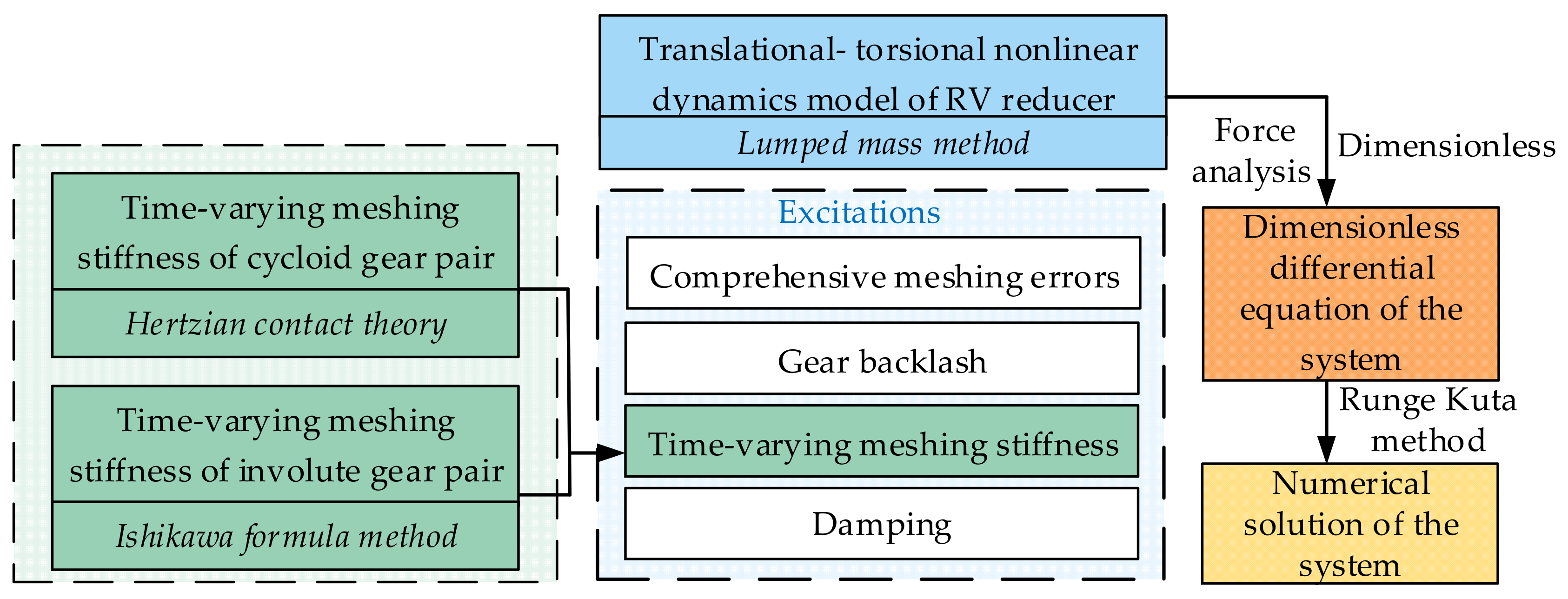
2. Translational–Torsional Nonlinear Dynamics Modeling of the RV Reducer

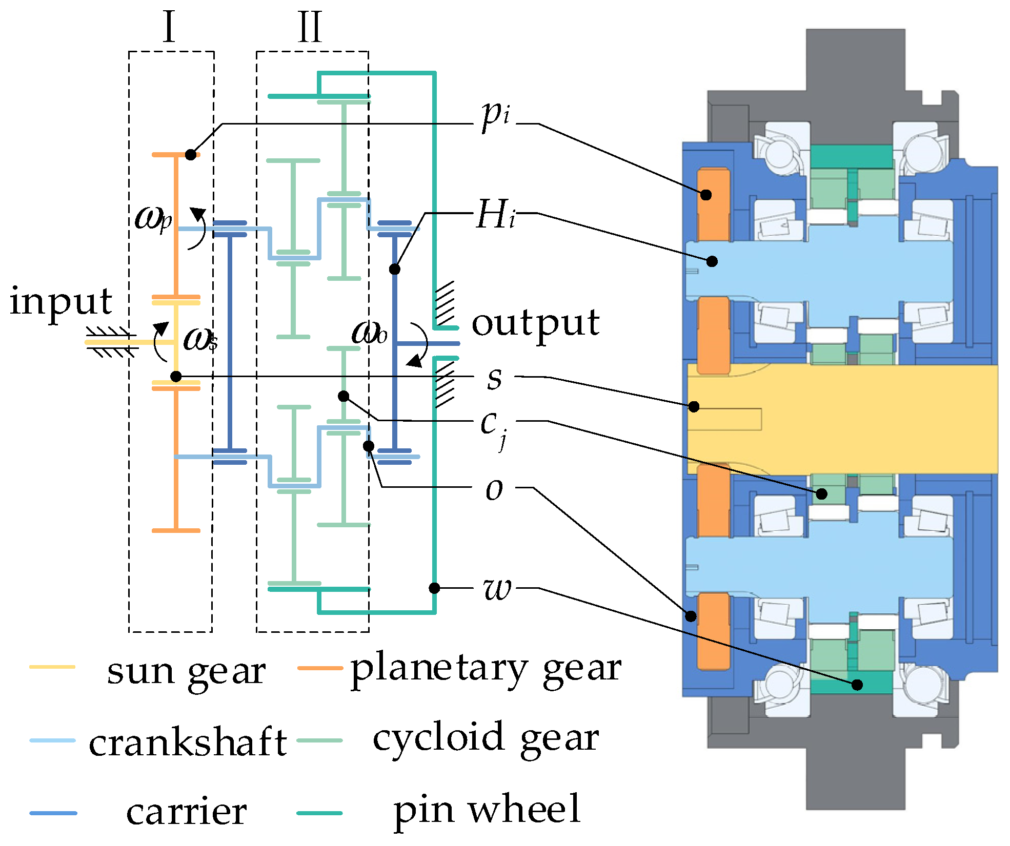
2.1. Structure and Transmission Principle of RV the Reducer

This paper takes RV reducers as the research object. As shown in Figure 1, the RV reducer transmission system mainly consists of an involute planetary gear system at the first level and a cycloidal pinwheel system at the second level with a small tooth difference, with a sun gear, a planetary gear, a crankshaft, a cycloid gear, a carrier, and a pinwheel as its core components. In Figure 1, $s,p_i,H_i,c_j,o,w$$(i=1,2,3;$$j=1,2)$ represent the $i$-th sun gear, the $i$-th planetary gear, the $i$-th crankshaft, the $j$-th cycloid gear, the carrier, and the pinwheel, respectively. ${\omega }_s$, ${\omega }_p$ and ${\omega }_o$ represent the rotation speed of the sun gear, the rotation speed of the planetary gear, and the rotation speed of the carrier, respectively.

In the operation process of RV reducers, with the movement from the sun gear input, the sun wheel experiences clockwise rotation with an angular velocity of ${\omega }_s$ driven by the planetary gear and crankshaft, and experiences counterclockwise rotation with an angular velocity of ${\omega }_p$, as the crankshaft and cycloid gears offset the phase and the distance is the same. Therefore, this constitutes a quadrilateral mechanism, causing the cycloid gear to experience counterclockwise rotation with an angular velocity of ${\omega }_p$ due to the simultaneous engagement of the cycloid gear and the pinwheel. Simultaneously, as the cycloid gear is subjected to a contact reaction force, the cycloid gear rotates clockwise with an angular velocity of ${\omega }_o$. The rotation of the cycloid gear drives the crankshaft to rotate clockwise with an angular velocity of ${\omega }_o$. The final movement is transferred to the carrier, which outputs the crankshaft rotation.

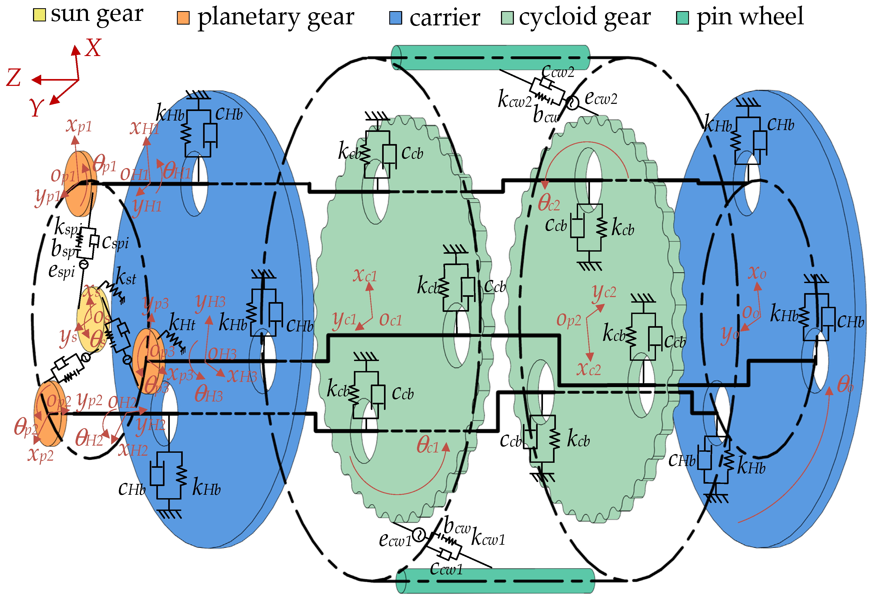
2.2. The Lumped Parameter Model of RV Reducer

Due to the high stiffness of each component of the RV reducer transmission system and the short axial spacing of each component, the lumped-mass method is used to establish the system translational–torsional dynamics model, as shown in Figure 2. Each active component has three degrees of freedom, two of which are translational and one of which is rotational.

Since the RV reducer described in this paper only considers the working condition of the fixed pinwheel housing and the output of the carrier, the center O of the needle tooth indexing circle is chosen as the origin of the global coordinate system, and X and Y are the horizontal and vertical directions, respectively. The origin of each local coordinate system in the system model is located at the geometric center of the corresponding component. The local coordinate system is divided into two types: (1) the central coordinate system $o{x}_s{y}_s$ and $o{x}_o{y}_o$, in which the x and y directions are the same as the global coordinate system; (2) the planetary coordinate system, $o{x}_{pi}{y}_{pi}$, $o{x}_{Hi}{y}_{Hi}$, and $o{x}_{cj}{y}_{cj}$, which rotates around the origin O of the global coordinate system with angular velocity ${\omega }_o$ and ${\omega }_p$, respectively. Its x direction is defined by the global coordinate system origin O pointing to the geometric center of each planetary component, and the y direction is defined by a 90° counterclockwise rotation in the x direction. ${\theta }_s$, ${\theta }_{pi}$, ${\theta }_{Hi}$, ${\theta }_{cj}$, and ${\theta }_o$ are the torsional angular displacement of the sun gear, the i-th planetary gear, the i-th crankshaft, the j-th cycloid gear, and the carrier.

In Figure 2, b_sp and b_cw are the half-tooth backlash of the involute gear pair and the cycloidal–pinwheel pair, respectively; $k_{st}$ and $k_{Ht}$ are the input shaft torsional stiffness and crankshaft torsional stiffness, respectively, which can be calculated from the shaft torsion angle; $k_s$ and $k_p$ are the sun gear support stiffness and planetary gear support stiffness, respectively, which can be calculated from the cantilever beam flexural deformation. $k_{spi}$ and $k_{cwj}$ are the time-varying mesh stiffness of the i-th involute gear pair and the time-varying mesh stiffness of the j-th cycloidal pinwheel pair; k_cb, k_Hb, and $k_o$ are the radial support stiffnesses of the support bearings between the eccentric shaft section of the crankshaft and the cycloidal gear, the support bearings between the non-eccentric part of the crankshaft end and the carrier, and the main bearings between the carrier and the pinwheel housing, respectively; these were calculated using the Palmgre formula [11,28,52,53], expressed as follows:

$$k_l=l^{0.8}{F}^{0.1}/\left[1.36{\left(h_1+h_2\right)}^{0.9}\right]\left(l=c,H,o\right),$$

(1)

$$h_i=\left(1-v_i^2\right)/\pi E_i,$$

(2)

where $E_i$ and $v_i$ represent the elastic modulus and Poisson’s ratio of the contact component material, respectively, $i=1,2$; $l$ represents the contact line length; and $F$ represents the load on the contact component.

$c_n$$(n=s,p,Hb,cb,o)$ represents the damping of support for each component, $c_n=\lambda m_n+\gamma k_n$, where $\lambda$ and $\gamma$ are the Rayleigh damping coefficients and $m_n$ is the mass of each component [54]; $c_{spi}$ and $c_{cwj}$ represent involute gear pair mesh damping and cycloid gear pair mesh damping, $c_{mn}=2{\xi }_{mn}\sqrt{k_{mn}/\left[1/m_1+1/m_2\right]}\left(mn=spi,cwj\right)$, where $\xi$ represents the meshing damping coefficient [55], $\xi$ can be taken as 0.03–0.17 [56], and $m_1$ and $m_2$ are the masses of the driving and driven gears, respectively.

${\theta }_m$($m=s,p_i,H_i,c_j,o$) represents the torsional angular displacement of each movable component. We convert the torsional displacement of each component into a line displacement u on the tangent line as follows:

$$\{\begin{array}{l}{u}_s=r_s{\theta }_s\\ u_{pi}=r_p{\theta }_{pi}\\ u_{Hi}=e{\theta }_{Hi}\\ u_{cj}=r_c{\theta }_{cj}\\ u_o=r_H{\theta }_o\end{array},$$

(3)

where $r_s$, $r_p$, e, $r_c$, and $r_H$ are the radius of the indexing circle of the sun gear and planetary gear, the crankshaft eccentricity distance, the radius of the distribution circle of the pinwheel, and the radius of the distribution circle of the crankshaft hole, respectively.

2.3. Time-Varying Meshing Stiffness of Gears

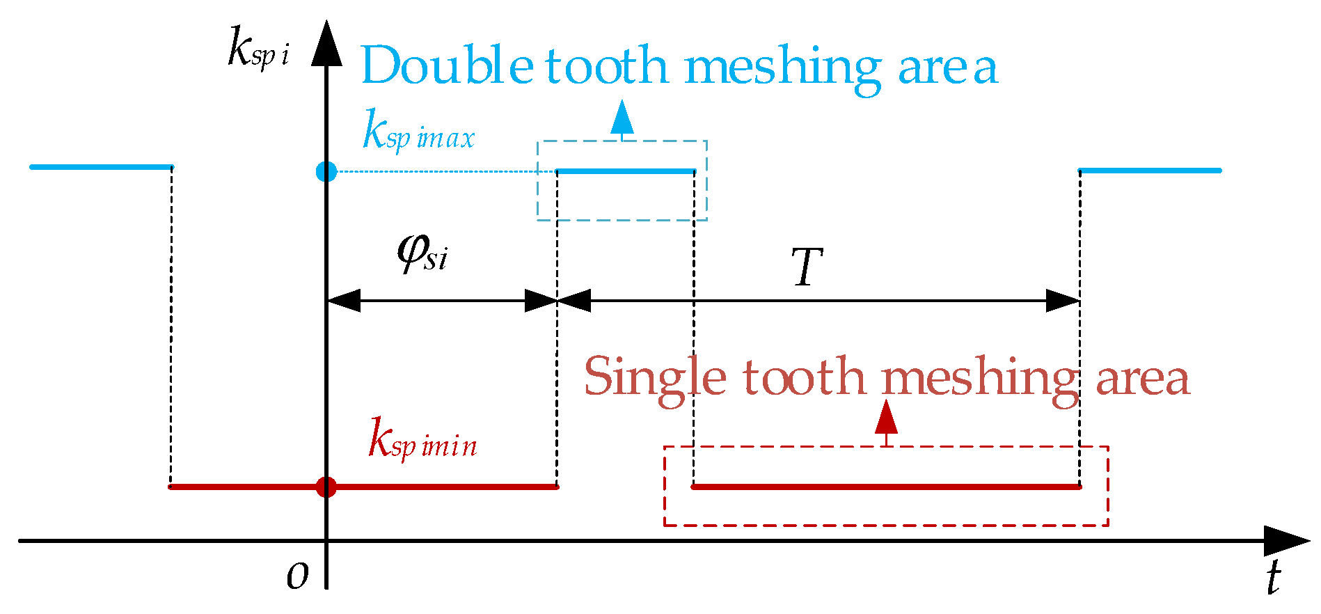
2.3.1. Time-Varying Meshing Stiffness of Involute Gear Pair

During the meshing of involute spur gears, single-tooth and double-tooth engagements alternate. The time-varying mesh stiffness exhibits an approximately periodic square wave pattern as the number of engaged gear pairs changes, as shown in Figure 3. In Figure 3, $k_{\mathit{spimax}}$ and $k_{\mathit{spimin}}$ are the maximum and minimum values of the time-varying meshing stiffness of an involute gear, ${\phi }_{si}$ is the phase of the i-th planetary gear, and T is the mesh cycle, ${\phi }_{si}=2\pi \left(i-1\right)/3$.

For the purpose of simplifying the computation, the time-varying mesh stiffness is approximated using a first-order Fourier series fit, represented as [57]

$$k_{spi}=k_{spm}+k_{spc}\cos \left({\omega }_{sp}t+{\phi }_{si}\right)$$

(4)

where $k_{spm}$ represents the mean value of the time-varying mesh stiffness for involute spur gears, which is calculated using the Ishikawa formula method [58], considering the mean value of mesh stiffness over one meshing cycle; $k_{spc}$ represents the Fourier coefficients of the time-varying mesh stiffness curve for involute spur gears;

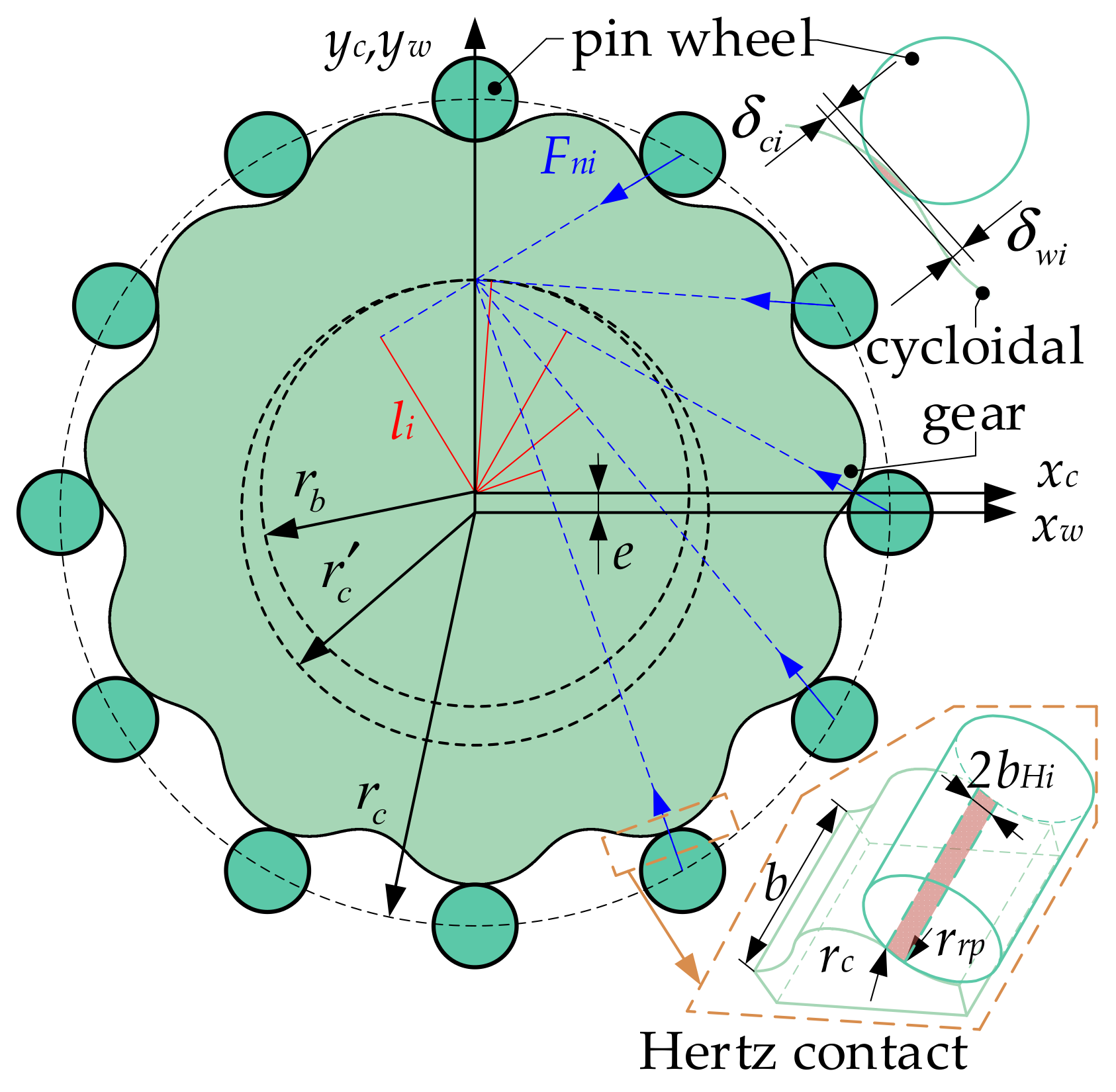
2.3.2. Time-Varying Meshing Stiffness of Cycloid Gear Pair

In Figure 4, the meshing model for the cycloidal pinwheel transmission is illustrated, which describes the stress and contact deformation of a cycloidal pinwheel during meshing. In Figure 4, $r_b$, $r_c^{\prime }$, and $r_{rp}$ are the radius of the cycloidal gear pitch circle, the radius of the pinwheel pitch circle, and the radius of the pinwheel, respectively; b is the tooth width of the cycloidal gear; $l_i$ is the moment arm of the contact force for the i-th pair of meshing tooth pairs in the cycloidal pinwheel pair; $F_{ni}$ is the contact force of the i-th pair of meshing tooth pairs in the cycloidal pinwheel pair; $k_{ci}$ and $k_{wi}$ are the contact stiffness of the cycloidal gear and the pinwheel.

During the meshing of the cycloidal pinwheel pair, multiple pairs of teeth are in contact, and the force situation is complex. Therefore, when calculating the time-varying mesh stiffness of the cycloidal pinwheel pair, it is necessary to first determine the number of meshing teeth. Subsequently, based on the Hertz contact theory, the Hertz contact half-width $b_{Hi}$ for each contacting tooth pair is computed. Consequently, the extrusion deformations for each contacting tooth pair of the cycloidal gear and pinwheel can be determined. According to Hooke’s law, the contact stiffness for the cycloidal gear and the pinwheel can be obtained upon this foundation. Considering these two contact stiffness values in series yields the single-tooth meshing stiffness $k_{cw}$ for each contacting tooth pair. Finally, by equivalently transforming the tooth contact stiffness of each contacting tooth pair into a single-tooth torsional stiffness and summing up the single-tooth torsional stiffness of each meshed tooth pair, the meshing stiffness of the cycloidal pinwheel pair can be determined.

The Hertz contact half-width for each contacting tooth pair can be expressed as:

$$b_{Hi}=\sqrt{\left(4F_{ni}{R}^{\prime }\right)/\left(\pi b{E}^{\prime }\right)}$$

(5)

where $1/E^{\prime }=\left(1-{\mu }_c^2\right)/E_c+\left(1-{\mu }_w^2\right)/E_w$; $1/R^{\prime }=1/r_{rp}+1/{\rho }_c$; ${\mu }_c$ and ${\mu }_w$ are the Poisson’s ratios of the cycloidal gear and pinwheel materials; $E_c$ and $E_w$ are the elastic moduli of the materials for the cycloidal gear and pinwheel; and ${\rho }_c$ is the curvature radius of the cycloidal gear.

The contact stiffness $k_{ci}$ for the cycloidal gear and contact stiffness $k_{wi}$ for the pinwheel can be expressed as:

$$k_{ci}=F_{ni}/{\delta }_{ci}=\pi b{E}_c{\rho }_c/\left[4R^{\prime }\left(1-{\mu }_c^2\right)\right]$$

(6)

$$k_{wi}=F_{ni}/{\delta }_{wi}=\pi b{E}_w{r}_{rp}/\left[4R^{\prime }\left(1-{\mu }_w^2\right)\right]$$

(7)

The single-tooth meshing stiffness $k_{cwti}$ for the i-th meshing tooth pair on the cycloidal pinwheel can be expressed as:

$$k_{cwti}=k_{ci}{k}_{wi}/\left(k_{ci}+k_{wi}\right)$$

(8)

The meshing stiffness $k_{cw}$ for a cycloidal pinwheel pair can be expressed as:

$$k_{cw}={\displaystyle \sum _{i=p}^q{k}_{cwti}{l}_i}$$

(9)

where p is the starting tooth pair number and q is the ending tooth pair number.

The fluctuation in the meshing stiffness of the cycloidal pinwheel pair is primarily caused by changes in the number of teeth, exhibiting periodic variations with the meshing frequency. To simplify calculations, a first-order Fourier series is employed to approximate the time-varying meshing stiffness $k_{cwj}$ for the cycloidal pinwheel pair, and can be expressed as [30]:

$$k_{cjr}=k_{cwjm}+k_{cwjc}\cos \left({\omega }_{cw}t+{\phi }_{cj}\right),$$

(10)

where $k_{cwjm}$ and $k_{cwjc}$ are the mean values of the time-varying meshing stiffness for the cycloidal pinwheel pair and Fourier coefficients; ${\omega }_{cw}$ is the meshing frequency for the cycloidal pinwheel pair, ${\omega }_{cw}=\left[Z_c\left({\omega }_p-{\omega }_o\right)\right]/2\pi$; $Z_c$ is the number of teeth on the cycloidal gear, and ${\phi }_{cj}$ is the phase angle of the cycloidal gear, ${\phi }_{cj}=\left(j-1\right)\pi$.

2.4. Relative Motion and Force Analysis between Movable Components in the RV Reducer Transmission System

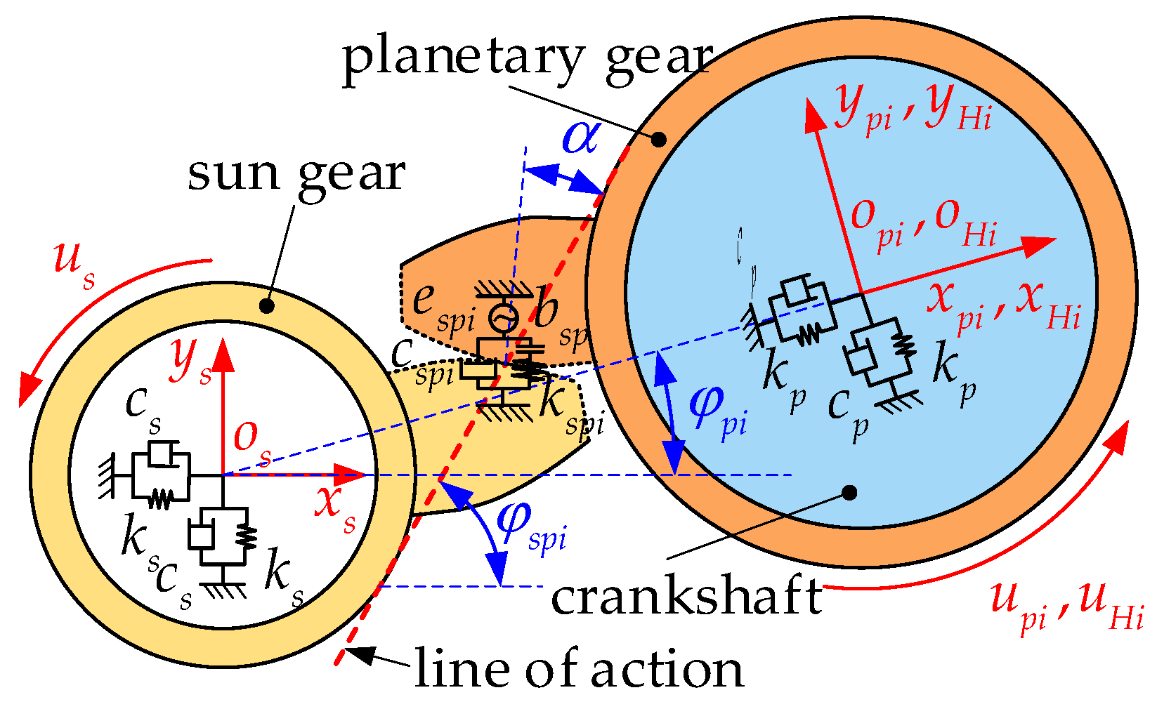
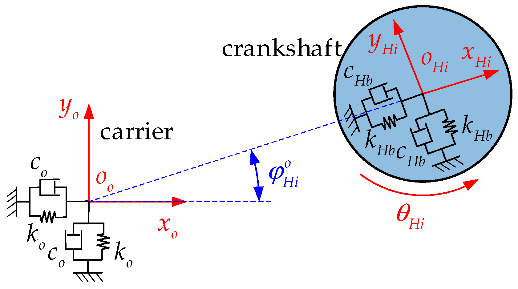
2.4.1. Relative Motion Relationship and Force Analysis in Planetary Gear System

To analyze the relative motion relationship between the sun gear and the planetary gear, as well as the force, the dynamic model of a planetary gear system is established, and it is assumed that the direction of the sun gear pointing to the planetary gear is the positive direction of relative displacement, as shown in Figure 5, where $\alpha$ is the pressure angle of involute gears, ${\phi }_{pi}$ is the position angle of the i-th planetary gear, and ${\phi }_{spi}$ is the angle between the mesh line of the i-th pair of involute gears and the $x_s$ axis, ${\phi }_{spi}=\alpha -{\phi }_{si}$.

The force of the sun gear at the support $F_{sx}$, $F_{sy}$, and the force due to the torsion of the input shaft $F_{su}$ can be expressed as

$$\{\begin{array}{l}{F}_{sx}=k_s{x}_s+c_s{\dot{x}}_s\\ F_{sy}=k_s{y}_s+c_s{\dot{y}}_s\\ F_{su}=k_{st}{u}_s+c_{st}{\dot{u}}_s\end{array}$$

(11)

By projecting the planar displacements ${\delta }_{si}$ and ${\delta }_{pi}$ of the sun gear and planetary gear onto the line of action, the relative displacement ${\delta }_{spi}$ between the sun gear and the i-th planetary gear can be expressed as:

$${\delta }_{spi}={\delta }_{si}-{\delta }_{pi}=\left(x_s\cos {\phi }_{si}+y_s\sin {\phi }_{si}+u_s\right)-\left(x_{pi}\sin \alpha +y_{pi}\cos \alpha -u_{pi}\right)+e_{spi},$$

(12)

where $e_{spi}$ represents the comprehensive meshing error for the i-th involute gear pair, which can be expressed as a sine function [44]:

$$e_{spi}=E_{sp}\sin ({\omega }_{sp}t+{\phi }_i)$$

(13)

where $E_{sp}$ represents the static transmission error of an involute gear pair.

Due to manufacturing and installation errors and the need for lubrication, clearances must be present between the gear teeth. To describe the influence of tooth clearances on the relative displacement ${\delta }_{spi}$ between the sun gear and the planetary gear, a piecewise function $f({\delta }_{spi},t)$ is employed to depict the relative displacement between the sun gear and the planetary gear, considering the effect of clearances [44].

$$f({\delta }_{spi},t)=\{\begin{array}{ll}{\delta }_{spi}-b_{sp},& \left({\delta }_{spi}>b_{sp}\right)\\ 0,& \left(\left|{\delta }_{spi}\right|\le b_{sp}\right)\\ {\delta }_{spi}+b_{sp},& \left({\delta }_{spi}<-b_{sp}\right)\end{array}$$

(14)

The meshing force for the i-th pair of involute gears can be expressed as:

$$F_{spi}=k_{spi}f({\delta }_{spi},t)+c_{spi}f({\dot{\delta }}_{spi},t)$$

(15)

The relative displacement of the planetary gear concerning the crankshaft in the $x_{Hi}$, $y_{Hi}$ and $u_{Hi}$ directions (${\delta }_{pHix}$, ${\delta }_{pHiy}$ and ${\delta }_{pHiu}$, respectively) can be expressed as:

$$\{\begin{array}{l}{\delta }_{pHix}=x_{pi}-x_{Hi}\\ {\delta }_{pHiy}=y_{pi}-y_{Hi}\\ {\delta }_{pHiu}=e{u}_{pi}/r_p-u_{Hi}\end{array}$$

(16)

The interaction forces $F_{pHix}$, $F_{pHiy}$ and $F_{pHiu}$ between the planetary gear and the crankshaft in the directions $x_{Hi}$, $y_{Hi}$ and $u_{Hi}$, respectively, can be expressed as:

$$\{\begin{array}{l}{F}_{pHix}=k_p{\delta }_{pHix}+c_p{\dot{\delta }}_{pHix}\\ F_{pHiy}=k_p{\delta }_{pHiy}+c_p{\dot{\delta }}_{pHiy}\\ F_{pHiu}=k_{Ht}{\delta }_{pHiu}+c_{Ht}{\dot{\delta }}_{pHiu}\end{array}$$

(17)

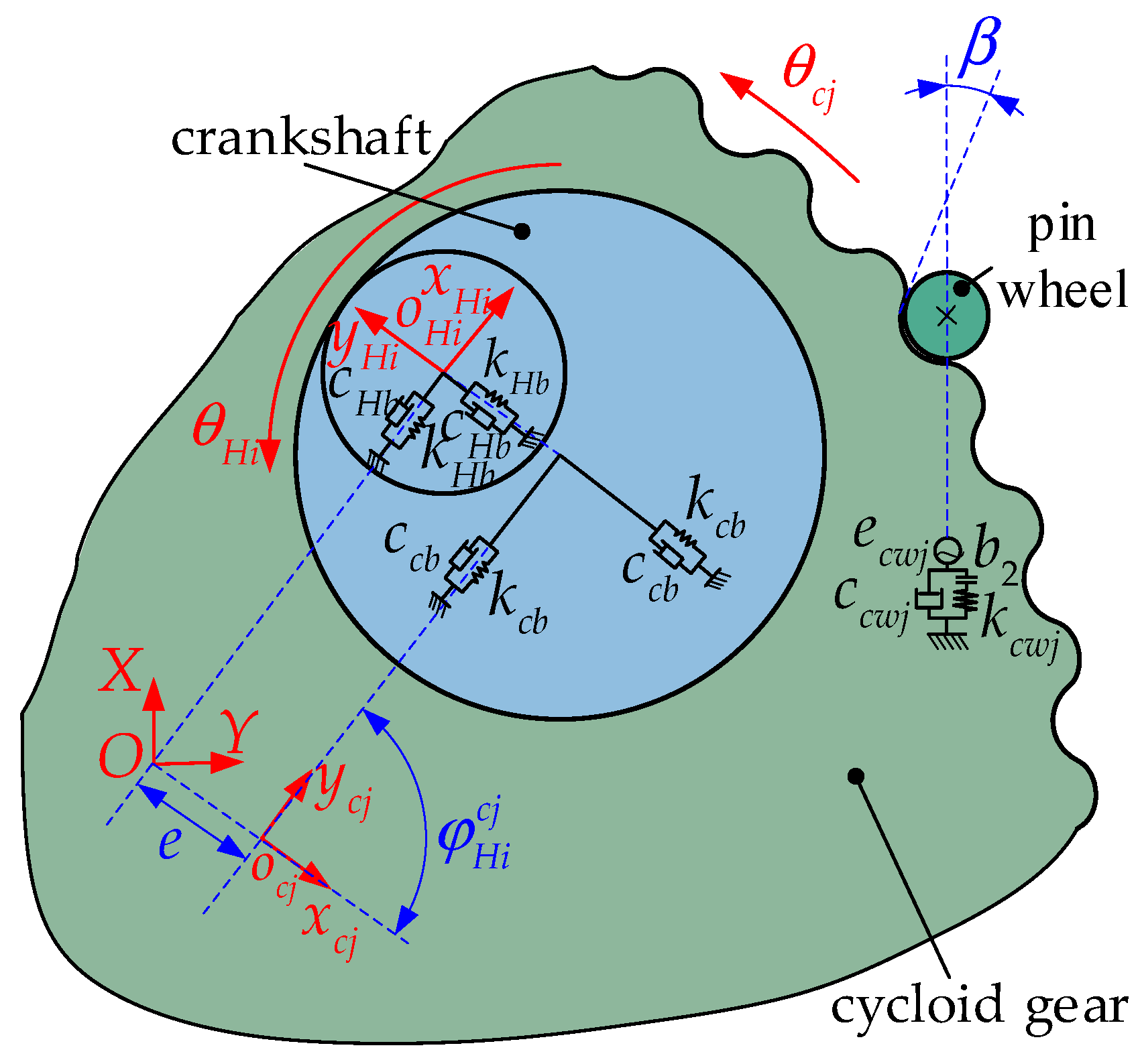
2.4.2. Relative Motion Relationship and Force Analysis in Cycloidal Pinwheel System

To analyze the relative motion relationship and relative force in the cycloidal pinwheel system, the dynamics model of the cycloidal pinwheel system is established by taking the j-th cycloidal gear as an example, as shown in Figure 6, where ${\phi }_{Hi}^{cj}$ is the angle between the $x$ direction of the j-th cycloidal gear and the $x$ direction of the i-th crankshaft, and $\beta$ is the equivalent pressure angle. Since the pinwheels are fixed on the pinwheel housing, the displacement of the pinwheel is zero. Therefore, by projecting the planar displacement of the cycloid gear onto the meshing line of the cycloid pinwheel, the relative displacement between the cycloid gear and the pinwheel can be expressed as:

$${\delta }_{cwj}=x_{cj}\sin \beta +y_{cj}\cos \beta +u_{cj}\cos \beta +e_{cwj}$$

(18)

where $e_{cwj}$ represents the comprehensive meshing error for the j-th cycloid pinwheel pair, which can be expressed as a sine function [30]:

$$e_{cwj}=E_{cw}\sin ({\omega }_{cw}t+{\phi }_j),$$

(19)

where $E_{cw}$ represents the static transmission error of the cycloid pinwheel pair.

Due to factors such as assembly errors, installation errors, and profile modifications, the cycloid pinwheel unavoidably exhibits tooth clearances. The clearance function can be expressed as follows [30]:

$$f({\delta }_{cwj},t)=\{\begin{array}{ll}{\delta }_{cwj}-b_{cw},& \left({\delta }_{cwj}>b_{cw}\right)\\ 0,& \left(\left|{\delta }_{cwj}\right|\le b_{cw}\right)\\ {\delta }_{cwj}+b_{cw},& \left({\delta }_{cwj}<-b_{cw}\right)\end{array}$$

(20)

The meshing force of the j-th cycloid pinwheel pair can be expressed as

$$F_{cwj}=k_{cwj}f({\delta }_{cwj},t)+c_{cwj}f({\dot{\delta }}_{cwj},t)$$

(21)

As shown in Figure 6, by projecting the plane displacements of the crankshaft and the cycloid gear in the $x_{Hi}$ and $y_{Hi}$ directions, the relative displacements ${\delta }_{Hix}^{cj}$ and ${\delta }_{Hiy}^{cj}$ of the cycloid gear relative to the crankshaft in the $x_{Hi}$ and $y_{Hi}$ directions can be obtained. They can be calculated using the following equations:

$$\{\begin{array}{l}{\delta }_{Hix}^{cj}=x_{Hi}+u_{Hi}\sin {\phi }_{Hi}^{cj}-x_{cj}\cos {\phi }_{Hi}^{cj}-y_{cj}\sin {\phi }_{Hi}^{cj}\\ {\delta }_{Hiy}^{cj}=y_{Hi}+u_{Hi}\cos {\phi }_{Hi}^{cj}+x_{cj}\sin {\phi }_{Hi}^{cj}-y_{cj}\cos {\phi }_{Hi}^{cj}-u_{cj}\cos {\phi }_{Hi}^{cj}\end{array}$$

(22)

The support forces $F_{Hix}^{cj}$ and $F_{Hiy}^{cj}$ of the crankshaft bearing in the $x_{Hi}$ and $y_{Hi}$ directions can be expressed as:

$$\{\begin{array}{l}{F}_{Hix}^{cj}=k_{cb}{\delta }_{Hix}^{cj}+c_{cb}{\dot{\delta }}_{Hiy}^{cj}\\ F_{Hiy}^{cj}=k_{cb}{\delta }_{Hiy}^{cj}+c_{cb}{\dot{\delta }}_{Hiy}^{cj}\end{array}$$

(23)

2.4.3. Relative Motion Relationship and Force Analysis at the Output Stage

Taking the i-th crankshaft as an example, the dynamic model of the output stage is established, as shown in Figure 7, where ${\phi }_{Hi}^o$ is the angle between the x direction of the planetary carrier and the x direction of the i-th crankshaft. By projecting the planar displacements of the crankshaft and planetary carrier in the $x_{Hi}$ and $y_{Hi}$ directions, respectively, the relative displacements of the planetary carrier with respect to the crankshaft in the $x_{Hi}$ and $y_{Hi}$ directions, ${\delta }_{Hix}^o$ and ${\delta }_{Hiy}^o$, are obtained, and can be expressed as

$$\{\begin{array}{l}{\delta }_{Hix}^o=x_{Hi}-x_o\cos {\phi }_{Hi}^o-y_o\sin {\phi }_{Hi}^o-u_o\sin {\phi }_{Hi}^o\\ {\delta }_{Hiy}^o=y_{Hi}+x_o\sin {\phi }_{Hi}^o-y_o\cos {\phi }_{Hi}^o-u_o\cos {\phi }_{Hi}^o\end{array}$$

(24)

The support forces $F_{Hix}^o$ and $F_{Hiy}^o$ of the support bearing in the $x_{Hi}$ and $y_{Hi}$ directions can be expressed as:

$$\{\begin{array}{l}{F}_{Hix}^o=k_{Hb}{\delta }_{Hix}^o+c_{Hb}{\dot{\delta }}_{Hix}^o\\ F_{Hiy}^o=k_{Hb}{\delta }_{Hiy}^o+c_{Hb}{\dot{\delta }}_{Hiy}^o\end{array}$$

(25)

The support forces $F_{ox}$ and $F_{oy}$ of the main bearing in the $x_o$ and $y_o$ directions can be expressed as:

$$\{\begin{array}{l}{F}_{ox}=k_o{x}_o+c_o{\dot{x}}_o\\ F_{oy}=k_o{y}_o+c_o{\dot{y}}_o\end{array}$$

(26)

2.5. System of Dimensionless Differential Equations

The dynamic system of RV gearbox transmission is derived based on Newton’s second law. Due to significant differences in the magnitudes of various physical quantities within this system of differential equations, substantial rounding errors are inevitably introduced. To enhance computational accuracy, the dimensional normalization of the parameters within the system of differential equations is necessary. The specific procedure is outlined as follows: By introducing dimensionless frequency ${\omega }_e$, ${\omega }_e=$$\sqrt{k_{spm}/m_e}$, $m_e=\frac{m_s{m}_p{m}_H{m}_c{m}_o}{m_s{m}_p{m}_H{m}_c+m_s{m}_p{m}_H{m}_o+m_p{m}_H{m}_c{m}_o+m_s{m}_p{m}_{c}m+m_s{m}_H{m}_c{m}_o}$, dimensionless time $\tau$, $\tau ={\omega }_{e}t$, and nominal length $b_c$, $b_c=10\mathsf{\mu }\mathrm{m}$, the dimensionless displacement $\overline{x}$, velocity $\dot{\overline{x}}$, acceleration $\ddot{\overline{x}}$, dimensionless mesh frequency ${\Omega }_c$ of the cycloidal needle gear, and the dimensionless frequency ${\Omega }_p$ of the involute meshed gear can be expressed as

$$\{\begin{array}{l}\overline{x}=x/b_c\\ \dot{\overline{x}}=\dot{x}/{\omega }_e/b_c\\ \ddot{\overline{x}}=\ddot{x}/{\omega }_e^2/b_c\\ {\mathsf{\Omega }}_c={\omega }_c/{\omega }_e\\ {\mathsf{\Omega }}_p={\omega }_p/{\omega }_e\end{array}$$

(27)

The dimensional comprehensive mesh error ${\overline{e}}_{pi}$ for the involute gear pair and the dimensional comprehensive mesh error ${\overline{e}}_{cj}$ for the cycloidal pinwheel pair can, respectively, be expressed as:

$${\overline{e}}_{pi}={\overline{E}}_p\sin ({\Omega }_p\tau +{\phi }_{pi})$$

(28)

$${\overline{e}}_{cj}={\overline{E}}_c\sin ({\Omega }_c\tau +{\phi }_{cj})$$

(29)

where ${\overline{E}}_p$ represents the dimensional static transmission error of the involute gear pair, ${\overline{E}}_p=E_p/b_c$, and ${\overline{E}}_c$ represents the dimensional static transmission error of the cycloidal pinwheel pair, ${\overline{E}}_c=E_c/b_c$.

The dimensional non-linear function of tooth clearance for the involute gear pair and cycloidal pinwheel pair can be expressed as:

$$f({\overline{\delta }}_k,t)=\{\begin{array}{ll}{\overline{\delta }}_k-{\overline{b}}_k,& \left({\overline{\delta }}_k>{\overline{b}}_k\right)\\ 0,& \left(\left|{\overline{\delta }}_k\right|\le {\overline{b}}_k\right)\\ {\overline{\delta }}_k+{\overline{b}}_k,& \left({\overline{\delta }}_k<-{\overline{b}}_k\right)\end{array}\left(k=spi,cwj\right)$$

(30)

where ${\overline{b}}_k$ represents the dimensional half-tooth clearance, ${\overline{b}}_k=b_k/b_c$.

By substituting Equations (27)–(30) into the dynamic differential equation set of the RV reducer transmission system and rearranging the deformations, the dimensionless dynamic differential equation set for the system can be expressed as

$$\{\begin{array}{l}{\ddot{\overline{x}}}_s+{\overline{F}}_{sx}+{\displaystyle \sum _{i=1}^3\left({\overline{F}}_{spi}\sin {\phi }_{si}\right)}=0\\ {\ddot{\overline{y}}}_s+{\overline{F}}_{sy}+{\displaystyle \sum _{i=1}^3\left({\overline{F}}_{spi}\cos {\phi }_{si}\right)}=0\\ {\ddot{\overline{u}}}_s+{\overline{F}}_{su}+{\displaystyle \sum _{i=1}^3{\overline{F}}_{spi}}={\overline{F}}_s\end{array},$$

(31)

$$\{\begin{array}{l}{\ddot{\overline{x}}}_{pi}+{\overline{F}}_{pHix}-{\overline{F}}_{spi}\sin \alpha =0\\ {\ddot{\overline{y}}}_{pi}+{\overline{F}}_{pHiy}-{\overline{F}}_{spi}\cos \alpha =0\\ {\ddot{\overline{u}}}_{pi}+e{\overline{F}}_{pHiu}/r_p+{\overline{F}}_{spi}=0\end{array},$$

(32)

$$\{\begin{array}{l}{\ddot{\overline{x}}}_{Hi}-{\overline{F}}_{pHix}+{\overline{F}}_{Hix}^o+{\displaystyle \sum _{j=1}^2{\overline{F}}_{Hix}^{cj}}=0\\ {\ddot{\overline{y}}}_{Hi}-{\overline{F}}_{pHiy}+{\overline{F}}_{Hiy}^o+{\displaystyle \sum _{j=1}^2{\overline{F}}_{Hiy}^{cj}}=0\\ {\ddot{\overline{u}}}_{Hi}-{\overline{F}}_{pHiu}+{\displaystyle \sum _{j=1}^2\left({\overline{F}}_{Hiy}^{cj}\cos {\phi }_{Hi}^{cj}+{\overline{F}}_{Hix}^{cj}\sin {\phi }_{Hi}^{cj}\right)}=0\end{array},$$

(33)

$$\{\begin{array}{l}{\ddot{\overline{x}}}_{cj}+{\overline{F}}_{cwj}\sin \beta -{\displaystyle \sum _{i=1}^3\left({\overline{F}}_{Hix}^{cj}\cos {\phi }_{Hi}^{cj}+{\overline{F}}_{Hiy}^{cj}\sin {\phi }_{Hi}^{cj}\right)}=0\\ {\ddot{\overline{y}}}_{cj}+{\overline{F}}_{cwj}\cos \beta +{\displaystyle \sum _{i=1}^3\left({\overline{F}}_{Hix}^{cj}\sin {\phi }_{Hi}^{cj}-{\overline{F}}_{Hiy}^{cj}\cos {\phi }_{Hi}^{cj}\right)}=0\\ {\ddot{\overline{u}}}_{cj}+{\overline{F}}_{cwj}\cos \beta -{\displaystyle \sum _{i=1}^3{r}_H{\overline{F}}_{Hiy}^{cj}/r_c}=0\end{array},$$

(34)

$$\{\begin{array}{l}{\ddot{\overline{x}}}_o+{\overline{F}}_{ox}-{\displaystyle \sum _{i=3}^3\left({\overline{F}}_{Hix}^o\cos {\phi }_{Hi}^o+{\overline{F}}_{Hiy}^o\sin {\phi }_{Hi}^o\right)}=0\\ {\ddot{\overline{y}}}_o+{\overline{F}}_{oy}+{\displaystyle \sum _{i=3}^3\left({\overline{F}}_{Hix}^o\sin {\phi }_{Hi}^o-{\overline{F}}_{Hiy}^o\cos {\phi }_{Hi}^o\right)}=0\\ {\ddot{\overline{u}}}_o-{\displaystyle \sum _{i=3}^3{\overline{F}}_{Hiy}^o}=-{\overline{F}}_o\end{array},$$

(35)

where, ${\overline{F}}_s=\frac{F_s}{m_s{b}_c{\omega }_e^2}$, ${\overline{F}}_o=\frac{F_o}{m_o{b}_c{\omega }_e^2}$, ${\overline{F}}_{sx}=\frac{F_{sx}}{m_s{b}_c{\omega }_e^2}$, ${\overline{F}}_{sy}=\frac{F_{sy}}{m_s{b}_c{\omega }_e^2}$, ${\overline{F}}_{su}=\frac{F_{su}}{I_s{b}_c{\omega }_e^2}$, ${\overline{F}}_{spi}=\frac{F_{spi}}{M_{sp}{b}_c{\omega }_e^2}$, ${\overline{F}}_{ox}=\frac{F_{ox}}{m_o{b}_c{\omega }_e^2}$, ${\overline{F}}_{oy}=\frac{F_{oy}}{m_o{b}_c{\omega }_e^2}$, ${\overline{F}}_{pHix}=\frac{F_{pHix}}{M_{pH}{b}_c{\omega }_e^2}$, ${\overline{F}}_{pHiy}=\frac{F_{pHiy}}{M_{pH}{b}_c{\omega }_e^2}$, ${\overline{F}}_{pHiu}=\frac{F_{pHiu}}{I_{pH}{b}_c{\omega }_e^2}$, ${\overline{F}}_{cwj}=\frac{F_{cwj}}{m_c{b}_c{\omega }_e^2}$, ${\overline{F}}_{Hix}^o=\frac{F_{Hix}^o}{M_{oH}{b}_c{\omega }_e^2}$, ${\overline{F}}_{Hiy}^o=\frac{F_{Hiy}^o}{M_{oH}{b}_c{\omega }_e^2}$, ${\overline{F}}_{Hiy}^{cj}=\frac{F_{Hiy}^{cj}}{M_{cH}{b}_c{\omega }_e^2}$, ${\overline{F}}_{Hix}^{cj}=\frac{F_{Hix}^{cj}}{M_{cH}{b}_c{\omega }_e^2}$, $M_{ij}=\frac{m_i{m}_j}{m_i+m_j}\left(i=s,p,H,c,o;j=s,p,H,c,o\right)$, and $I_{pH}=\frac{I_p{I}_H}{I_s+I_H}$.

3. Nonlinear Dynamic Analysis of RV Reducer

To analyze the evolution of motion states in the RV reducer transmission system globally, clarify the nonlinear dynamic characteristics, and delineate chaotic regions, initially, a bifurcation diagram for the system is generated. Subsequently, analyses of the phase trajectory, Poincaré sections, and power spectrum are conducted for specific parameters to scrutinize the dynamic response qualitatively. This methodology aims to determine the motion states of the system further, and enhance understanding of its nonlinear dynamics.

The standard three-crankshaft RV-80E reducer was chosen as the research subject in this paper. The geometric design parameters for this reducer are presented in

Table 1. Basic parameters of the gear.

Types of Gears	Design Parameters	Value
Involute gear	Number of sun gear teeth Zs	12
	Number of planetary gear teeth Zp	36
	Modulus m (mm)	1.5
	Meshing angle $\alpha$ ($°$)	20
Cycloidal pinwheel	Number of pinwheels Zw	40
	Number of cycloidal gear teeth Zc	39
	Eccentricity distance e (mm)	1.3
	Pin position radius rc (mm)	85.8

, while the mass and moment of inertia for each component are outlined in

Table 2. Masses and moment of inertia of components in the RV reducer.

Name of the Component	Symbol	Mass (kg)	Moment of Inertia (kg·m2)
Sun gear (s)	ms	1.30	$4.44\times {10}^{-4}$
Planetary gear (p)	mp	0.88	$1.01\times {10}^{-3}$
Crankshaft (H)	mH	0.40	$7.56\times {10}^{-5}$
Cycloidal gear (c)	mc	2.76	$2.09\times {10}^{-2}$
Carrier (o)	mo	15.33	$1.06\times {10}^{-1}$

. Additionally, the stiffness parameters within the system are detailed in

Table 3. Stiffness parameters in the RV reducer transmission system.

Parameter Name	Value
kspm (N·m−1)	$2.38\times {10}^8$
kcrm (N·m−1)	$1.27\times {10}^9$
kcb (N·m−1)	$9.84\times {10}^8$
kHb (N·m−1)	$9.76\times {10}^8$
ko (N·m−1)	$1.51\times {10}^9$
ks (N·m−1)	$1.23\times {10}^8$
kp (N·m−1)	$5.55\times {10}^8$
kst (N·m/rad)	$1.16\times {10}^4$
kHt (N·m/rad)	$6.99\times {10}^4$

. The input torque in the system is denoted as $T_s=412 \mathrm{N}\cdot \mathrm{m}$ and the output torque is represented as $T_o=3.4 \mathrm{N}\cdot \mathrm{m}$. Two excitation frequencies, ${\Omega }_p$ and ${\Omega }_c$, are present, with the condition ${\Omega }_p=3{\Omega }_c/5$. The Runge–Kutta method is employed to solve the dimensionless differential equation system. To ensure that the computed results do not include transient responses, the bifurcation diagram, phase trajectory, and Poincaré section are generated using the results obtained after 1000 response cycles.

The process of establishing and solving the nonlinear dynamic model is shown in Figure 8.

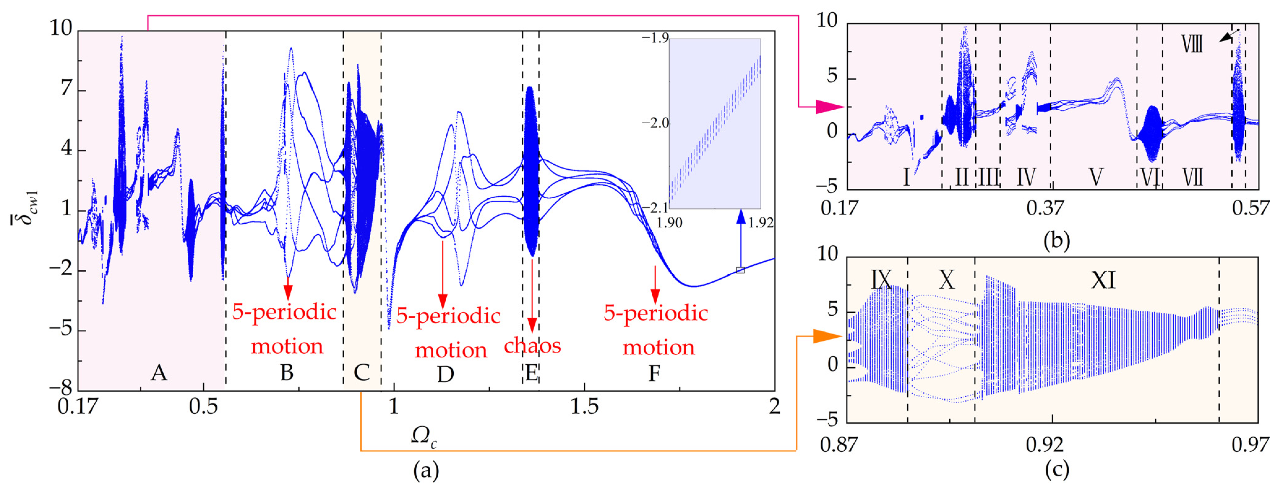
3.1. Dynamic Response of the System with the Variation of Excitation Frequency

The dimensional static transmission errors of the involute gear pair and the cycloidal pinwheel pair are set as ${\overline{E}}_{sp}={\overline{E}}_{cw}=5$, with dimensional half-tooth clearance ${\overline{b}}_{sp}={\overline{b}}_{cw}=3$ between the involute gear pair and the cycloidal pinwheel pair. The meshing damping coefficient is set as ${\xi }_{sp}={\xi }_{cr}=0.1$, and the initial displacement and velocity are set to 0. The dimensional meshing frequency of the cycloidal pinwheel pair increases from 0.17 to 2. After preliminary calculations, the relative displacement motion changes along the meshing lines of each gear pair are roughly similar. Therefore, taking the dimensional relative displacement between the cycloidal gear and the pinwheel as an example, the bifurcation diagram of the system with the dimensional meshing frequency ${\Omega }_c$ of the cycloidal pinwheel pair is shown in Figure 9. The following text is simplified for the description, referring to the dimensional meshing frequency of the cycloidal pinwheel pair as the excitation frequency. The bifurcation diagram of the system with variations in the excitation frequency is divided into six regions labeled as A, B, C, D, E, and F, as shown in Figure 9a. The excitation frequency intervals corresponding to each region are outlined in

Table 4. Excitation frequency intervals for regions A to F.

Regions Code	Frequency Interval
Regions A	$\left[0.17,0.5572\right)$
Regions B	$\left[0.5572,0.8651\right)$
Regions C	$\left[0.8651,0.9607\right)$
Regions D	$\left[0.9607,1.3365\right)$
Regions E	$\left[1.3365,1.3795\right)$
Regions F	$\left[1.3795,2\right]$

. Due to the relatively complex nature of the motion states in regions A and C, local magnifications of these regions can be obtained separately, as shown in the local magnification diagrams in Figure 9b, c. Subsequently, these two regions are further subdivided into eleven subregions, labeled as I to XI, corresponding to the respective numbered regions in Figure 9b (I to VIII) and Figure 9c (IX to XI).

As shown in Figure 9a, in region A, the system exhibits complex and varied motion states, undergoing repetitive transitions between multi-periodic motion, quasi-multi-periodic motion, and chaotic motion. Within region I, where the excitation frequency ${\Omega }_c\in \left[0.17,0.2619\right)$, the system undergoes a transition from periodic motion to quasi-periodic motion, exhibiting intermittent chaos. When ${\Omega }_c\in \left[0.17,0.2013\right)$, the system is in a five-period motion state, and when ${\Omega }_c=0.2013$, it undergoes a fold bifurcation and enters a 10-period motion state. In Figure 10 and Figure 11, corresponding to ${\Omega }_c=0.2012$ and ${\Omega }_c=0.2013$, the phase trajectory, Poincaré sections, and power spectrum are presented. At this point, the system exhibits a multi-periodic motion state, where the phase trajectory consists of n closed loops (n is the number of periods), the Poincaré section shows n stable fixed points, and the power spectrum is distributed at positions corresponding to $1/n$ and $m/n$ (where m is a positive integer).

As the excitation frequency increases, when ${\Omega }_c=0.2120$, the system undergoes a brief quasi-periodic motion before returning to a five-period motion state. Subsequently, at the excitation frequency of ${\Omega }_c\in \left[0.2121,0.2265\right)$, the system consistently remains in a five-period motion state. Continuing to vary the excitation frequency, when the excitation frequency is in the interval $\left[0.2265,0.2282\right]$, the system exhibits a quasi-periodic route to chaos. When ${\Omega }_c=0.2263$, the system is in a five-periodic motion state. At this point, the Poincaré section exhibits five stable fixed points, and the power spectrum is distributed at $1/5$ and $m/5$ (where m is a positive integer), as illustrated in Figure 12a and Figure 13a. Subsequently, when ${\Omega }_c=0.2265$, the system undergoes a Hopf bifurcation, entering into quasiperiodic motion. When the system is in a quasiperiodic five-period motion state, the Poincaré section exhibits five closed limit cycles (Figure 12b), and the power spectrum, in addition to being distributed at $1/5$ and $m/5$, also shows peaks at a series of irreducible frequency components and their linear combinations (Figure 13b). When ${\Omega }_c\in \left[0.2267,0.2282\right)$, the system is in a quasiperiodic five-period motion state. During this period, the limit cycles continuously expand and distort (Figure 12c,d), and additional irreducible frequency components appear on the power spectrum (Figure 13c,d). Eventually, when ${\Omega }_c=0.2282$, the phenomenon of limit cycle bursting occurs, and the system displays chaotic motion. At this point, the Poincaré section reveals a strange attractor with a fractal structure (Figure 12e), and the power spectrum exhibits a continuous spectrum resembling background noise (Figure 13e), with observable peaks significantly reduced.

Subsequently, when the excitation frequency ${\Omega }_c\in \left[0.2282,0.2619\right)$, the system undergoes repeated transitions between quasi-periodic motion and chaos. During this process, the system is in a chaotic state when the excitation frequency is in the relevant interval. The system is in a quasi-periodic motion state when the excitation frequency is in the remaining intervals. Finally, the system transitions into chaos through the intermittency route when ${\Omega }_c=0.2619$.

In region II, where the excitation frequency ${\Omega }_c\in \left[0.2619,0.2939\right)$, the system is in a chaotic state. During this period, two periodic windows exist, located at ${\Omega }_c\in \left[0.2812,0.2814\right)$ and ${\Omega }_c\in \left[0.2902,0.2095\right)$. Specifically, when ${\Omega }_c\in \left[0.2812,0.2814\right)$, the system displays a periodic window for a 10-period motion state, and when ${\Omega }_c\in \left[0.2902,0.2095\right)$, the system displays a periodic window for a 20-period motion state.

Examining a point in each of the two intervals, ${\Omega }_c=0.2813$ and ${\Omega }_c=0.2904$, the phase trajectory, Poincaré sections, and power spectrum are observed, as shown in Figure 14 and Figure 15. The Poincaré sections reveal 10 and 20 stable fixed points, while the power spectrum exhibit peaks at points $1/10$, $1/20$, $m/10$, and $m/20$.

In region III, the excitation frequency of the system is in the interval $\left[0.2939,0.3187\right)$. When ${\Omega }_c=0.2939$, the system transitions from chaos back to quasiperiodic five-period motion. Subsequently, the system enters a five-period motion state through a reverse Hopf bifurcation, ${\Omega }_c=0.2949$. After that, the system remains in a five-period motion state within this region.

In region IV, the excitation frequency of the system is in the interval $\left[0.3187,0.3680\right)$. During this period, the motion state of the system undergoes transitions between multiperiodic motion and multi quasi-periodic motion. When ${\Omega }_c=0.3187$, the system undergoes a Hopf bifurcation, transitioning from five-period motion to quasiperiodic five-period motion. With an increase in excitation frequency, the motion state experiences a sudden change at ${\Omega }_c=0.3234$, shifting from quasiperiodic five-period motion to chaos. The corresponding phase trajectory, Poincaré section, and power spectrum are illustrated in Figure 16. At this point, the phase trajectory tends to fill a portion of space, and a fractal-shaped strange attractor emerges on the Poincaré section. The power spectrum exhibits a continuous spectrum in the vicinity of $12/15$. Additionally, peaks in the power spectrum are observed at points $1/15$ and $m/15$, indicating that the Poincaré section periodically visits 15 chaotic regions. The system undergoes a brief period of chaos and abruptly transitions to 15-period motion when ${\Omega }_c=0.3239$. Subsequently, the system remains in 15-period motion as the excitation frequency varies within the interval $\left[0.3239,0.3339\right]$. When ${\Omega }_c\in \left[0.3340,0.3409\right)$, the system undergoes Hopf bifurcation, transitioning into quasiperiodic 15-period motion. As the excitation frequency varies within the interval $\left[0.3410,0.3542\right]$, the system reverts to 15-period motion. When ${\Omega }_c=0.3543$, the motion state undergoes another abrupt transition into chaos, as illustrated in Figure 17 by the corresponding phase trajectory, Poincaré section, and power spectrum. When ${\Omega }_c\in \left[0.3548,0.3680\right)$, the system reverts to quasiperiodic five-period motion. The motion states in the remaining regions V–VIII in Figure 9b are straightforward and can be readily observed. Therefore, the motion states in regions V–VIII are provided directly in

Table 5. Excitation frequency intervals for regions V to VIII.

Region Code	Frequency Interval	Motion State
Regions V	$\left[0.3680,0.4572\right)$	5 periodic motion
Regions VI	$\left[0.4572,0.4761\right)$	5 quasi-periodic motion
Regions VII	$\left[0.4762,0.5436\right)$	5 periodic motion
Regions VIII	$\left[0.5436,0.5571\right]$	chaos

.

The motion states of the system in regions B, D, and F are singular, characterized by five-period motion. In these regions, the system uniformly undergoes transitions into periodic motion through inverse Hopf bifurcations and transitions into quasiperiodic motion through Hopf bifurcations. Therefore, the subsequent discussion will not redundantly elaborate on the dynamic response variations in regions B, D, and F, focusing solely on the dynamic response changes in regions C and E.

In region C, the system exhibits periodic motion, quasiperiodic motion, and chaos. Specifically, in sub-region IX, where ${\Omega }_c\in \left[0.8651,0.8847\right)$, the system is in a chaotic state, and in this region, the system transitions into chaos through the quasiperiodic route. In region X, where ${\Omega }_c\in \left[0.8847,0.9011\right)$, the system is in a periodic motion state. In region XI, where ${\Omega }_c\in \left[0.901,0.9606\right)$, the motion state alternates between quasiperiodic motion and chaos. In region E, the system exhibits a chaotic state. Upon observing its Poincaré section, it is evident that the system undergoes a transition from five-period motion (Figure 18a) to quasiperiodic motion with five periods (Figure 18b) through a Hopf bifurcation. The limit cycle undergoes continuous distortion and entanglement with increasing excitation frequency (Figure 18c). At ${\Omega }_c=1.3418$, the system experiences phase locking, manifesting as 125-period motion (Figure 18d), and eventually enters chaos at ${\Omega }_c=1.3419$ (Figure 18e). The corresponding power spectrum during the transition to chaos is depicted in Figure 19. It can be observed that as the system evolves from periodic to chaotic motion, the power spectrum shifts from having peaks at only $1/5$ and $m/5$ to exhibiting a continuous spectrum.

In particular, the bifurcation diagram (Figure 9a) shows that the system seems to enter into a single-period motion when the excitation frequency is in the relevant interval. However, upon closer inspection via a local magnification of the bifurcation diagram in this interval $\left[1.75,2\right]$, we see that the Poincaré section for this interval still falls within a relatively narrow region. To further validate the motion state in this interval, the phase trajectory, Poincaré sections, and power spectrum are generated for ${\Omega }_c=1.92$, as shown in Figure 20. The phase trajectory exhibits five closed loops, the Poincaré section reveals five stable fixed points, and the power spectrum is distributed at $1/5$ and $m/5$. This indicates that the system is in a five-period motion state rather than a single-period motion state when ${\Omega }_c\in \left[1.75,2\right]$.

Chaos means that the movement of the system is unpredictable and unrepeatable, and this is generally accompanied by an increase in the vibration amplitude of the system. This will deteriorate the performance of the RV reducer transmission system. From the perspective of engineering applications, the excitation frequency changes due to input speed. Therefore, the appropriate speed should be selected in practical applications to prevent the system from entering into chaos.

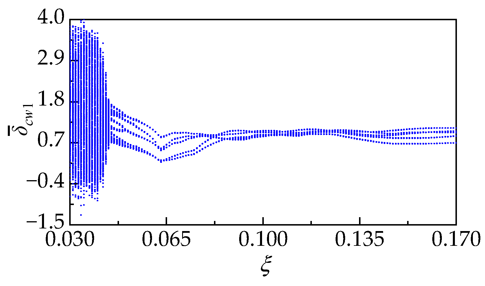
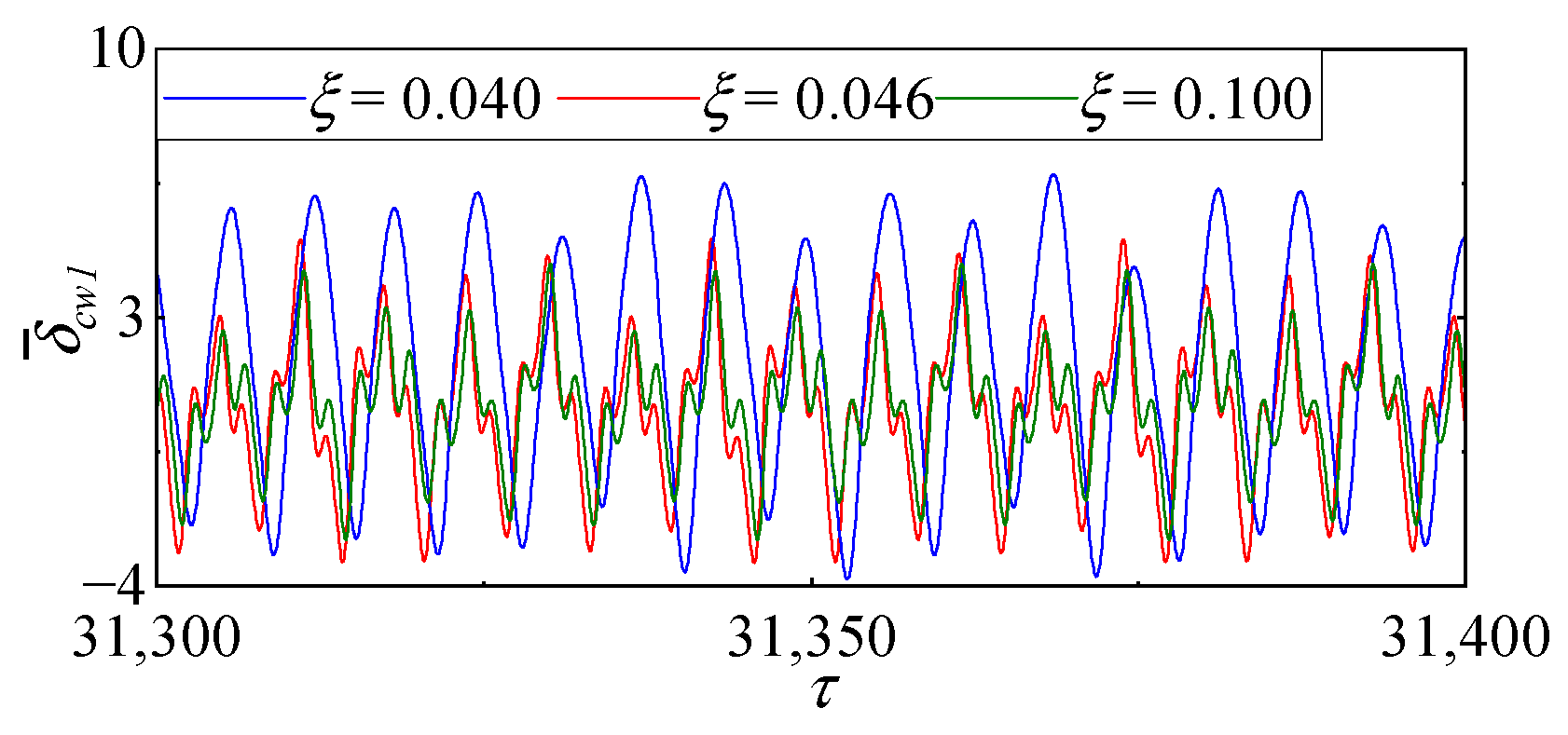
3.2. Dynamic Response of the System with Variation of Mesh Damping

The dimensional static transmission errors of the involute gear pair and the cycloidal pinwheel pair are set as ${\overline{E}}_{sp}={\overline{E}}_{cw}=5$, with dimensional half-tooth clearance ${\overline{b}}_{sp}={\overline{b}}_{cw}=3$ between the involute gear pair and the cycloidal pinwheel pair, and the excitation frequency is set as ${\Omega }_c=0.5$, while the initial displacement and velocity are set to 0. To investigate the evolution of the dynamic response as both meshing damping coefficients ${\xi }_{sp}$ and ${\xi }_{cw}$ simultaneously increase from 0.03 to 0.17, a bifurcation diagram is constructed, as illustrated in Figure 21. Since ${\xi }_{sp}$ and ${\xi }_{cw}$ change simultaneously and are of equal magnitude, they will be collectively referred to as the meshing damping coefficient, denoted as $\xi$ in the following text.

In Figure 21, when $\xi \in \left[0.030,0.045\right)$, the system exhibits chaotic behavior; when $\xi \in \left[0.045,0.049\right)$, the system displays quasiperiodic motion; and when $\xi \in \left[0.049,0.170\right]$, the system displays five-period motion. Parameters are selected within each motion regime, specifically $\xi =0.040$, $\xi =0.046$, and $\xi =0.100$. The corresponding phase trajectories and power spectrum for each set of parameters are depicted in Figure 22a,b, while the corresponding time domain plots are shown in Figure 23.

In Figure 22, with the increase in the damping coefficient $\xi$, the phase trajectories transition from a highly disordered state to regular closed loops. Simultaneously, the power spectrum tends to be distributed around $1/5$ and $m/5$, indicating that with the increase in the damping coefficient $\xi$, the motion state shifts from chaos to periodic motion.

In Figure 23, when $\xi =0.04$, $\xi =0.046$, and $\xi =0.100$, the vibration amplitudes are 7.66, 5.21, and 4.40, respectively. During the increase in meshing damping from 0.04 to 0.1, the vibration amplitude of the system decreases by 3.27, with a reduction of 42.69%.

As can be seen from Figure 22 and Figure 23, increasing the meshing damping coefficient can significantly reduce the vibration amplitude of the system. Additionally, certain chaos intervals of the system will gradually transition to quasi-periodic and periodic motion, indicating that an increase in damping effectively suppresses the occurrence of chaos.

4. Conclusions

The vibration differential equation of the RV reducer transmission system considering the gear backlash was derived and numerically solved. The bifurcation and chaos characteristics of the system were analyzed with the excitation frequency and meshing damping as control parameters. The following conclusions can be drawn:

(1)

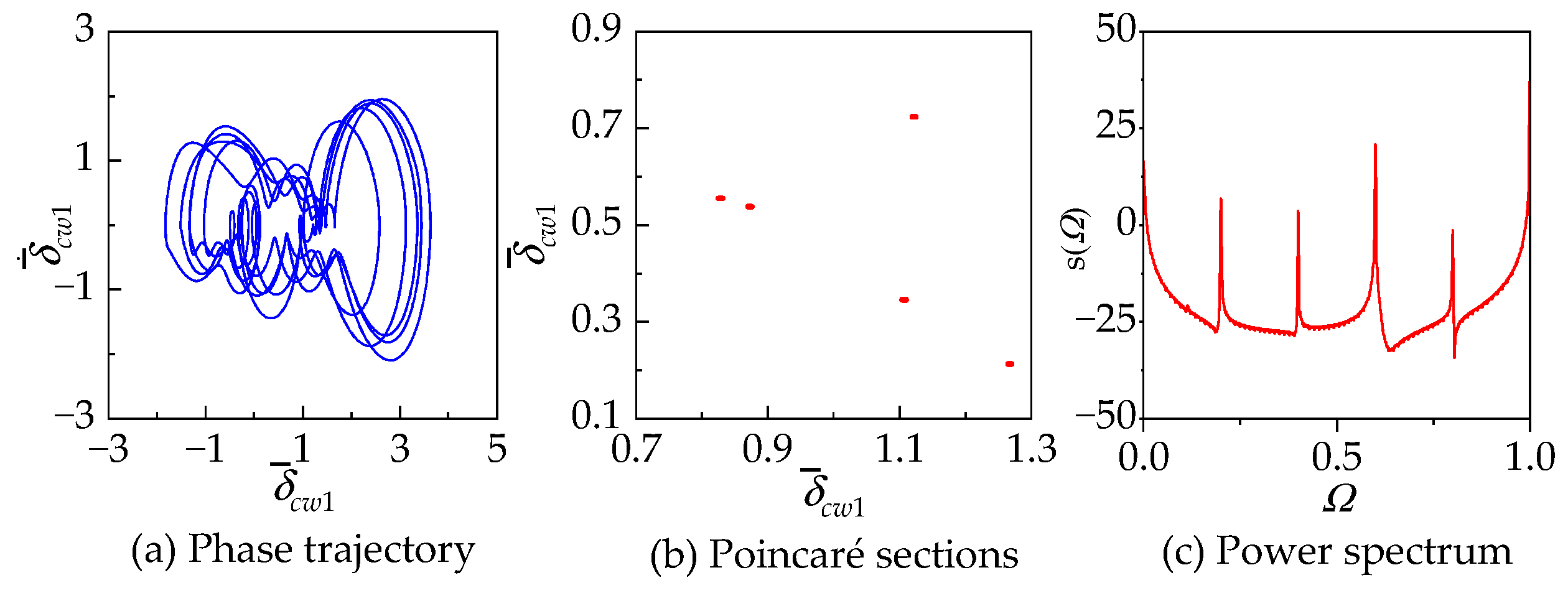
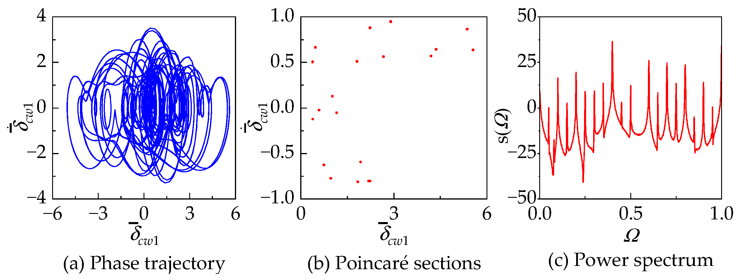
Considering gear backlash, time-varying mesh stiffness, and comprehensive meshing errors, a translational–torsional dynamic model of the RV reducer transmission system was established. The dimensionless vibration differential equations of the system were derived and solved numerically. The results provided by calculating bifurcation diagrams, phase portraits, Poincaré sections, and the power spectrum are illustrated clearly in order to analyze the motion states and chaotic regions of this system, and to investigate the effects of the excitation frequency and meshing damping coefficient;

(2)

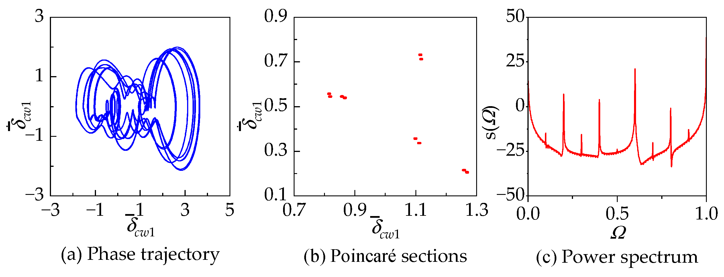
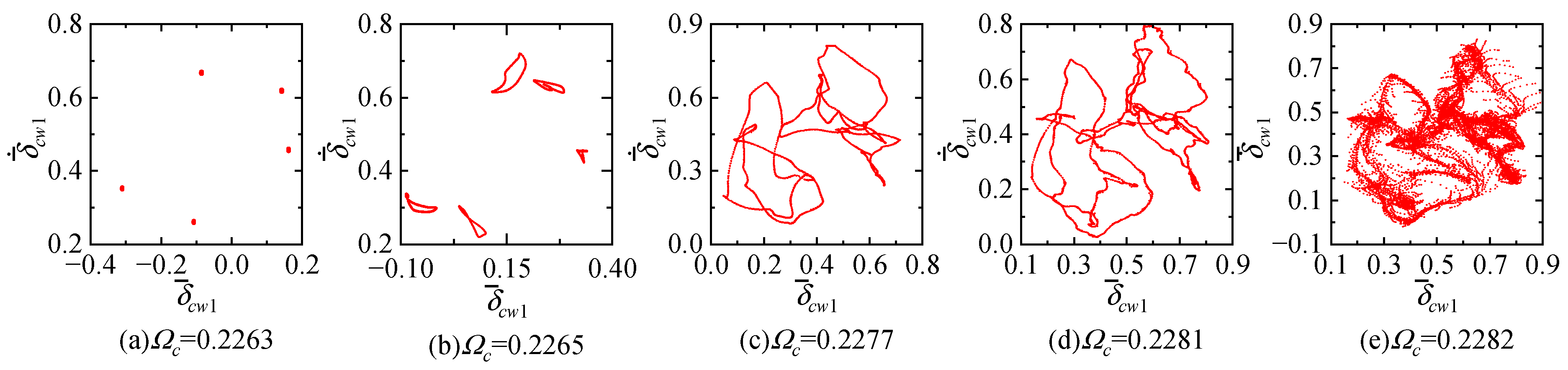
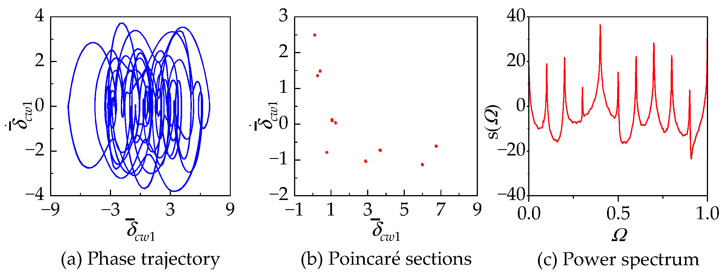
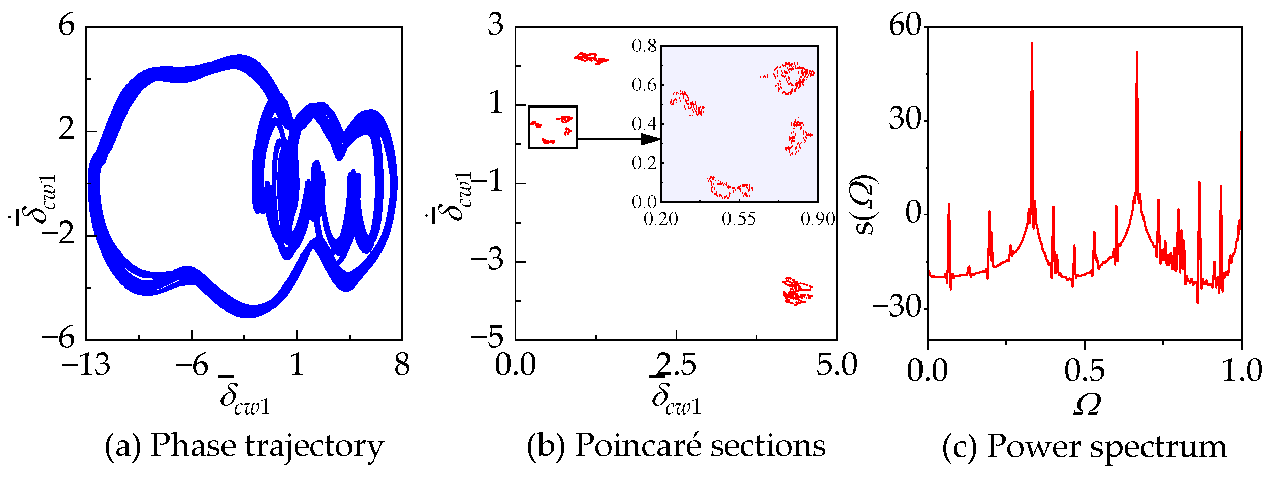
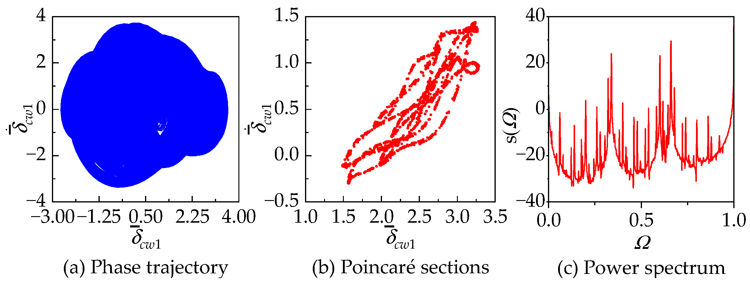
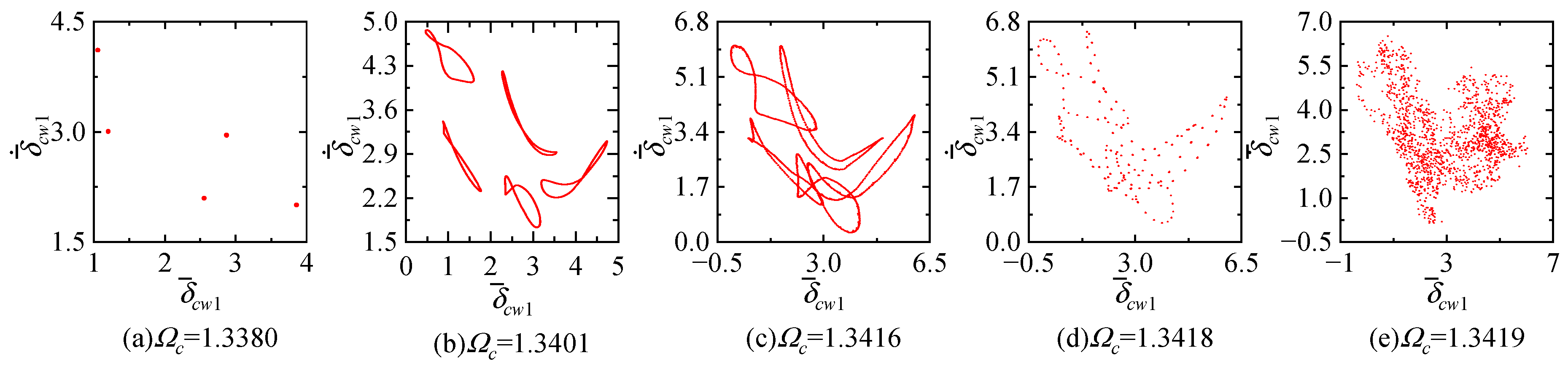
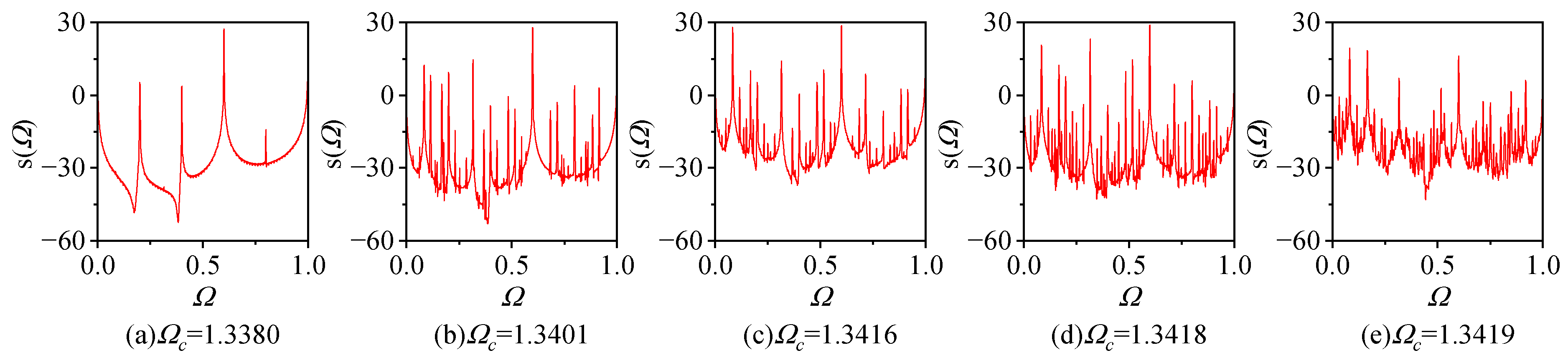
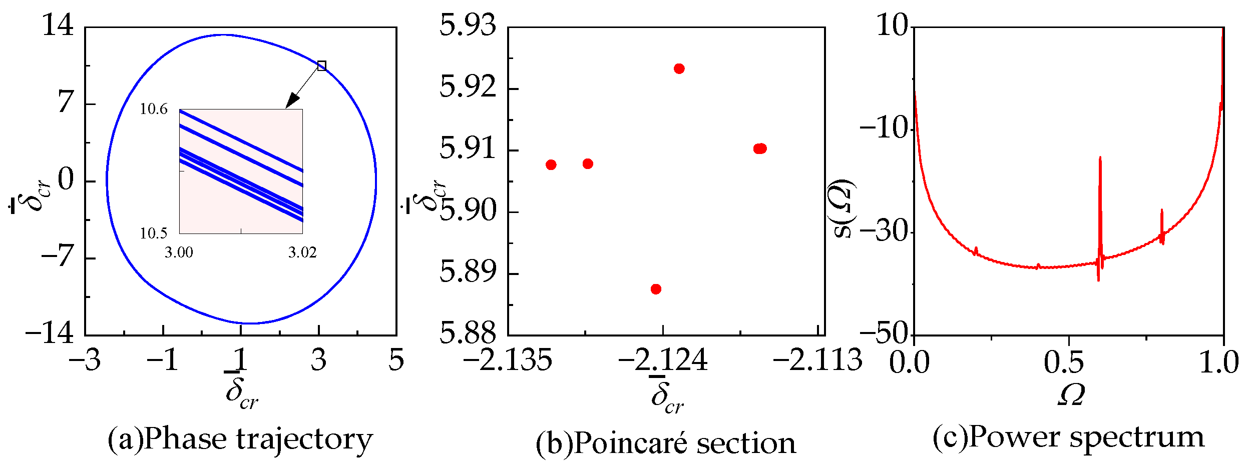
Altering the excitation frequency induces changes in the motion states, marked by the occurrence of fold bifurcation, Hopf bifurcation, and inverse Hopf bifurcation, leading to variations between periodic and quasiperiodic motions. Several conventional routes to chaos emerge throughout this process, including the quasiperiodic route, boundary crisis route, and intermittency route. This underscores that the RV reducer transmission system exhibits a wealth of nonlinear dynamic characteristics under factors such as time-varying mesh stiffness, errors, and backlash;

(3)

In the low-frequency range (${\Omega }_c\in \left[0.17,0.5771\right)$), the motion states of the system are more intricate and variable compared to the high-frequency range (${\Omega }_c\in \left[0.5771,2\right]$). Consequently, when the system operates in the low-frequency range, even slight variations in the excitation frequency can alter its motion states, making it more prone to entering chaotic intervals. Therefore, the prolonged operation of the RV reducer at low speeds should be avoided. At the same time, when designing RV reducer transmission systems, appropriately enhancing the meshing damping can significantly reduce the vibration of the system and improve system stability.

In this study, the translational torsional nonlinear dynamics model of an RV reducer was established, and the chaos and bifurcation characteristics of an RV reducer were analyzed, which provides a foundation for stability control and dynamic performance optimization of RV reducers. On the basis of the research in this study, more internal and external excitations can be considered, such as friction, wear and torque changes. This will make the analysis more accurate.

References

1. Pham, A.D.; Ahn, H.J. High Precision Reducers for Industrial Robots Driving 4th Industrial Revolution: State of Arts, Analysis, Design, Performance Evaluation and Perspective. Int. J. Precis. Eng. Manuf.-Green Technol. 2018, 5, 519–533. [Google Scholar] [CrossRef]
2. Yang, Y.H.; Zhou, G.C.; Chang, L.; Chen, G. A Modelling Approach for Kinematic Equivalent Mechanism and Rotational Transmission Error of RV Reducer. Mech. Mach. Theory 2021, 163, 104384. [Google Scholar] [CrossRef]
3. Matejic, M.; Blagojevic, M.; Disic, A.; Matejic, M.; Milovanovic, V.; Miletic, I. A Dynamic Analysis of the Cycloid Disc Stress-Strain State. Appl. Sci. 2023, 13, 4390. [Google Scholar] [CrossRef]
4. Stanojević, M.; Tomović, R.; Ivanović, L.; Stojanović, B. Critical Analysis of Design of Ravigneaux Planetary Gear Trains. Appl. Eng. Lett. J. Eng. Appl. Sci. 2022, 7, 32–44. [Google Scholar] [CrossRef]
5. Jia, J.S.; Zhou, J.X.; Zeng, Q.F.; Cui, Q.W.; Zhang, R.H.; Wei, Z. Review of RV Reducers with Precision Gear Transmission. Mach. Tool Hydraul. 2023, 51, 189–196. [Google Scholar] [CrossRef]
6. Hidaka, T.; Wang, H.; Ishida, T.; Matsumoto, K.; Hashimoto, M. Rotational Transmission Error of K-H-V Planetary Gears with Cycloid Gear: 1st Report, Analytical Method of the Rotational Transmission Error. Trans. Jpn. Soc. Mech. Eng. Ser. C 1994, 60, 645–653. [Google Scholar] [CrossRef]
7. Ishida, T.; Wang, H.; Hidaka, T.; Hashimoto, M. Rotational Transmission Error of K-H-V-Type Planetary Gears with Cycloid Gears: 2nd Report, Effects of Manufacturing and Assembly Errors on Rotational Transmission Error. Trans. Jpn. Soc. Mech. Eng. Ser. C 1994, 60, 3510–3517. [Google Scholar] [CrossRef]
8. Ren, Z.Y.; Mao, S.M.; Guo, W.C.; Guo, Z. Tooth Modification and Dynamic Performance of the Cycloidal Drive. Mech. Syst. Signal Process 2017, 85, 857–866. [Google Scholar] [CrossRef]
9. Zhang, R.H.; Zhou, J.X.; Wei, Z. Study on Transmission Error and Torsional Stiffness of RV Reducer under Wear. J. Mech. Sci. Technol. 2022, 36, 4067–4081. [Google Scholar] [CrossRef]
10. Xu, L.X.; Xia, C.; Yang, B. Analysis and Test on Dynamic Transmission Errors of RV Reducers under Load Conditions. China Mech. Eng. 2023, 34, 2143–2152. [Google Scholar] [CrossRef]
11. Wei, Z.; Zhou, J.X.; Cui, Q.W.; Jia, J.S.; Zhang, R.H.; Liu, G.C. A Method to Analyze Dynamic Transmission Error of RV Reducer Considering Machining Error and Flexible Factors. J. Xi’an Jiaotong Univ. 2023, 57, 161–172. [Google Scholar] [CrossRef]
12. Li, X.; Huang, J.Q.; Ding, C.C.; Guo, R.; Niu, W.L. Dynamic Modeling and Analysis of an RV Reducer Considering Tooth Profile Modifications and Errors. Machines 2023, 11, 626. [Google Scholar] [CrossRef]
13. Jiang, Z.H.; Zhang, X.L.; Liu, J.Q. A Reliability Evaluation Method for RV Reducer by Combining Multi-Fidelity Model and Bayesian Updating Technology. IOP Conf. Ser. Mater. Sci. Eng. 2021, 1043, 052038. [Google Scholar] [CrossRef]
14. Wang, H.L.; Fu, W.H.; Fang, K.; Chen, T.C. Transmission Characteristics of an RV Reducer Based on ADAMS. J. Mech. Sci. Technol. 2024, 38, 787–802. [Google Scholar] [CrossRef]
15. Wang, Z.H.; Xu, R.; Pan, J.B.; Chen, Q.Q.; Zhang, J.; Wang, J.G. Effect of Multifactor Interaction on the Accuracy of RV Reducers. Int. J. Rotating Mach. 2023, 2023, 5692229. [Google Scholar] [CrossRef]
16. Zhang, Y.H.; Xiao, J.J.; He, W.D. Dynamical Formulation and Analysis of RV Reducer. In Proceedings of the 2009 International Conference on Engineering Computation, Hong Kong, China, 2–3 May 2009; IEEE: Piscataway, NJ, USA, 2009; pp. 201–204. [Google Scholar] [CrossRef]
17. Zhang, Y.H.; He, W.D.; Xiao, J.J. Dynamical Model of RV Reducer and Key Influence of Stiffness to the Nature Character. In Proceedings of the 2010 Third International Conference on Information and Computing, Wuxi, China, 4–6 June 2010; IEEE: Piscataway, NJ, USA, 2010; pp. 192–195. [Google Scholar] [CrossRef]
18. Chen, C.; Yang, Y.H. Structural Characteristics of Rotate Vector Reducer Free Vibration. Shock Vib. 2017, 2017, 4214370. [Google Scholar] [CrossRef]
19. Pan, W.; Zhang, H.; Chen, C. Effect of Mesh Phasing on Dynamic Response of Rotate Vector Reducer. Int. J. Ind. Syst. Eng. 2021, 1, 190–209. [Google Scholar] [CrossRef]
20. Wang, S.; Tan, J.; Gu, J.J.; Huang, D.S. Study on Torsional Vibration of RV Reducer Based on Time-Varying Stiffness. J. Vib. Eng. Technol. 2021, 9, 73–84. [Google Scholar] [CrossRef]
21. Zhang, D.Q.; Li, X.A.; Yang, M.D.; Wang, F.; Han, X. Non-Random Vibration Analysis of Rotate Vector Reducer. J. Sound Vib. 2023, 542, 117380. [Google Scholar] [CrossRef]
22. Xu, L.; Xia, C.; Chang, L. Dynamic Modeling and Vibration Analysis of an RV Reducer with Defective Needle Roller Bearings. Eng. Fail. Anal. 2024, 157, 107884. [Google Scholar] [CrossRef]
23. Xu, L.X.; Chen, B.K.; Li, C.Y. Dynamic Modelling and Contact Analysis of Bearing-Cycloid-Pinwheel Transmission Mechanisms Used in Joint Rotate Vector Reducers. Mech. Mach. Theory 2019, 137, 432–458. [Google Scholar] [CrossRef]
24. Xu, L.X. A Study on Dynamic Load Characteristics of Multi-group Needle Roller Bearings Used in RV Reducer Considering the Position Errors. China Mech. Eng. 2022, 58, 144–155. [Google Scholar] [CrossRef]
25. Zheng, J.K.; Wang, H.; Kumar, A.; Xiang, J.W. Dynamic Model-Driven Intelligent Fault Diagnosis Method for Rotary Vector Reducers. Eng. Appl. Artif. Intell. 2023, 124, 106648. [Google Scholar] [CrossRef]
26. Shan, L.; He, W. Study on Nonlinear Dynamics of RV Transmission System Used in Robot Joints. In Recent Advances in Mechanism Design for Robotics; Bai, S., Ceccarelli, M., Eds.; Mechanisms and Machine Science; Springer International Publishing: Cham, Switzerland, 2015; Volume 33, pp. 317–324. ISBN 978-3-319-18125-7. [Google Scholar]
27. Shan, L.J.; Fang, X.; He, W.D. Nonlinear Dynamic Model and Equations of RV Transmission System. Adv. Mater. Res. 2012, 510, 536–540. [Google Scholar] [CrossRef]
28. Han, L.S.; Shen, Y.W.; Dong, J.H.; Wang, G.F.; Liu, J.Y.; Qi, H.J. Theoretical Research on Dynamic Transmission Accuracy for 2K-V Type Drive. J. Mech. Eng. 2007, 43, 81–86. [Google Scholar] [CrossRef]
29. Zheng, Y.X.; Xi, Y.; Bu, W.H.; LI, M.R. Nonlinear Characteristic Analysis of 5-degree-of-freedom Pure Torsional Model of RV Reducer. J. Zhejiang Univ. (Eng. Sci.) 2018, 52, 2098–2109+2119. [Google Scholar] [CrossRef]
30. Zheng, Y.X.; Wang, X.; Xi, Y.; Liu, J.S. Nonlinear Characteristics Analysis of Translational-Torsional Coupled Dynamic Model of RV Reducer. In Proceedings of the 2019 International Conference on Advances in Construction Machinery and Vehicle Engineering, Changsha, China, 14–16 May 2019; IEEE: Piscataway, NJ, USA, 2020. [Google Scholar] [CrossRef]
31. Blankenship, G.W.; Kahraman, A. Steady State Forced Response of a Mechanical Oscillator with Combined Parametric Excitation and Clearance Type Non-Linearity. J. Sound Vib. 1995, 185, 743–765. [Google Scholar] [CrossRef]
32. Kahraman, A.; Blankenship, G.W. Experiments on Nonlinear Dynamic Behavior of an Oscillator with Clearance and Periodically Time-Varying Parameters. J. Appl. Mech. 1997, 64, 217–226. [Google Scholar] [CrossRef]
33. Kahraman, A.; Blankenship, G.W. Effect of Involute Contact Ratio on Spur Gear Dynamics. J. Mech. Des. 1999, 121, 112–118. [Google Scholar] [CrossRef]
34. Byrtus, M.; Zeman, V. On Modeling and Vibration of Gear Drives Influenced by Nonlinear Couplings. Mech. Mach. Theory 2011, 46, 375–397. [Google Scholar] [CrossRef]
35. Margielewicz, J.; Gąska, D.; Litak, G. Modelling of the Gear Backlash. Nonlinear Dyn. 2019, 97, 355–368. [Google Scholar] [CrossRef]
36. Chen, S.Y.; Tang, J.Y.; Luo, C.W.; Wang, Q.B. Nonlinear Dynamic Characteristics of Geared Rotor Bearing Systems with Dynamic Backlash and Friction. Mech. Mach. Theory 2011, 46, 466–478. [Google Scholar] [CrossRef]
37. Wang, Z.Z.; Pu, W.; Pei, X.; Cao, W. Nonlinear Dynamical Behaviors of Spiral Bevel Gears in Transient Mixed Lubrication. Tribol. Int. 2021, 160, 107022. [Google Scholar] [CrossRef]
38. Chen, Q.; Wang, Y.D.; Tian, W.F.; Wu, Y.M.; Chen, Y.L. An Improved Nonlinear Dynamic Model of Gear Pair with Tooth Surface Microscopic Features. Nonlinear Dyn. 2019, 96, 1615–1634. [Google Scholar] [CrossRef]
39. Sakaridis, E.; Spitas, V.; Spitas, C. Non-Linear Modeling of Gear Drive Dynamics Incorporating Intermittent Tooth Contact Analysis and Tooth Eigenvibrations. Mech. Mach. Theory 2019, 136, 307–333. [Google Scholar] [CrossRef]
40. Al-Shyyab, A.; Kahraman, A. A Non-Linear Dynamic Model for Planetary Gear Sets. Proc. Inst. Mech. Eng. Part K J. Multi-Body Dyn. 2007, 221, 567–576. [Google Scholar] [CrossRef]
41. Ambarisha, V.K.; Parker, R.G. Nonlinear Dynamics of Planetary Gears Using Analytical and Finite Element Models. J. Sound Vib. 2007, 302, 577–595. [Google Scholar] [CrossRef]
42. Li, S.; Wu, Q.M.; Zhang, Z.Q. Bifurcation and Chaos Analysis of Multistage Planetary Gear Train. Nonlinear Dyn. 2013, 75, 217–233. [Google Scholar] [CrossRef]
43. Wang, J.G.; Zhang, W.; Long, M.; Liu, D.J. Study on Nonlinear Bifurcation Characteristics of Multistage Planetary Gear Transmission for Wind Power Increasing Gearbox. IOP Conf. Ser. Mater. Sci. Eng. 2018, 382, 042007. [Google Scholar] [CrossRef]
44. Liu, S.X.; Hu, A.J.; Sun, Y.Y.; Xiang, L.; Zhu, Y.C. Chaos and Impact Characteristics Analysis of a Multistage Planetary Gear System Based on the Energy Method. Int. J. Bifurc. Chaos 2023, 33, 2350046. [Google Scholar] [CrossRef]
45. Liu, S.X.; Hu, A.; Zhang, Y.; Xiang, L. Nonlinear Dynamics Analysis of a Multistage Planetary Gear Transmission System. Int. J. Bifurc. Chaos 2022, 32, 2250096. [Google Scholar] [CrossRef]
46. Xiang, L.; Liu, S.X.; Zhang, J.H. Nonlinear Dynamic Characteristics of Two-stage Planetary Gear Transmissionsystem in Wind Turbinegearbox. J. Vib. Shock 2020, 39, 193–199+229. [Google Scholar] [CrossRef]
47. Yang, R.G.; Han, B.; Li, F.P.; Zhou, Y.Q.; Xiang, J.W. Nonlinear Dynamic Analysis of a Trochoid Cam Gear. J. Mech. Des. 2020, 142, 094502. [Google Scholar] [CrossRef]
48. Yang, R.G.; Li, F.P.; Zhou, Y.Q.; Xiang, J.W. Nonlinear Dynamic Analysis of a Cycloidal Ball Planetary Transmission Considering Tooth Undercutting. Mech. Mach. Theory 2020, 145, 103694. [Google Scholar] [CrossRef]
49. Yang, R.G.; An, Z.J.; Jiang, W. Bifurcation Characteristics Study of Cycloid Ball Planetary Transmission. J. Vib. Shock 2017, 36, 134–140. [Google Scholar] [CrossRef]
50. Yang, R.G.; An, Z.J. Theoretical Calculation and Experimental Verification of the Elastic Angle of a Cycloid Ball Planetary Transmission Based on the Axial Pretightening Force. Adv. Mech. Eng. 2017, 9, 168781401773411. [Google Scholar] [CrossRef]
51. Chen, Z.M.; Ou, Y.; Long, S.Y.; Peng, W.H.; Yang, Z.X. Vibration Characteristics Analysis of the New Pin-Cycloid Speed Reducer. J. Braz. Soc. Mech. Sci. Eng. 2018, 40, 55. [Google Scholar] [CrossRef]
52. Palmgren, A.; Ruley, B. Ball and Roller Bearing Engineering; SKF Industries Inc.: Philadelphia, PA, USA; Burbank, CA, USA, 1959. [Google Scholar]
53. Jia, J.S.; Zhou, J.X.; Zeng, Q.F.; Li, G.K.; Wang, H.W.; Zhang, R.H. Research on the Influence of Flexible Factors on Dynamic Transmission Error in RV Reducer. Mach. Tool Hydraul. 2023, 51, 158–165. [Google Scholar] [CrossRef]
54. Yoshida, N.; Kobayashi, S.; Suetomi, I.; Miura, K. Equivalent Linear Method Considering Frequency Dependent Characteristics of Stiffness and Damping. Soil Dyn. Earthq. Eng. 2002, 22, 205–222. [Google Scholar] [CrossRef]
55. Lin, H.H.; Liou, C.H. A Parametric Study of Spur Gear Dynamics; University of Memphis: Memphis, TN, USA, 1998. [Google Scholar]
56. Yi, Y.Y.; Qin, D.T.; Liu, C.Z. Investigation of Electromechanical Coupling Vibration Characteristics of an Electric Drive Multistage Gear System. Mech. Mach. Theory 2018, 121, 446–459. [Google Scholar] [CrossRef]
57. Xiang, L.; Gao, N.; Hu, A.J. Dynamic Analysis of a Planetary Gear System with Multiple Nonlinear Parameters. J. Comput. Appl. Math. 2018, 327, 325–340. [Google Scholar] [CrossRef]
58. Shi, J.; Ma, X.; Xu, C.; Zang, S. Meshing Stiffness Analysis of Gear Using the Ishikawa Method. Appl. Mech. Mater. 2013, 401–403, 203–206. [Google Scholar] [CrossRef]
Figure 1. Schematic diagram of RV reducer transmission system structure.
Energies 17 01178 g001
Figure 2. Lumped parameter model of RV reducer.
Energies 17 01178 g002
Figure 3. Variation rule of time-varying mesh stiffness.
Energies 17 01178 g003
Figure 4. Meshing model of cycloid pinwheel transmission.
Energies 17 01178 g004
Figure 5. Dynamic model of planetary gear system.
Energies 17 01178 g005
Figure 6. Dynamic model of the cycloid pinwheel system.
Energies 17 01178 g006
Figure 7. Dynamic model of the output stage.
Energies 17 01178 g007
Figure 8. The flowchart of obtaining the numerical solution.
Energies 17 01178 g008
Figure 9. Bifurcation diagram for Ω c versus δ ¯ c 1 r with E ¯ s p = E ¯ c w = 5 , b ¯ s p = b ¯ c w = 3 , and ξ s p = ξ c r = 0.1 : (a) Ω c [ 0.17 ,   2 ] , (b) Ω c [ 0.17 ,   0.57 ] , (c) Ω c [ 0.87 ,   0.97 ] .
Energies 17 01178 g009
Figure 10. The periodic response of the system at Ω c = 0.2012 with E ¯ s p = E ¯ c w = 5 , b ¯ s p = b ¯ c w = 3 , and ξ s p = ξ c r = 0.1 .
Energies 17 01178 g010
Figure 11. The periodic response of the system at Ω c = 0.2013 with E ¯ s p = E ¯ c w = 5 , b ¯ s p = b ¯ c w = 3 , and ξ s p = ξ c r = 0.1 .
Energies 17 01178 g011
Figure 12. Phase trajectories of the system at Ω c [ 0.2263 ,   0.2282 ] with E ¯ s p = E ¯ c w = 5 , b ¯ s p = b ¯ c w = 3 , and ξ s p = ξ c r = 0.1 .
Energies 17 01178 g012
Figure 13. Power spectrum of the system at Ω c [ 0.2263 ,   0.2282 ] with E ¯ s p = E ¯ c w = 5 , b ¯ s p = b ¯ c w = 3 , and ξ s p = ξ c r = 0.1 .
Energies 17 01178 g013
Figure 14. The periodic response of the system at Ω c = 0.2813 with E ¯ s p = E ¯ c w = 5 , b ¯ s p = b ¯ c w = 3 , and ξ s p = ξ c r = 0.1 .
Energies 17 01178 g014
Figure 15. The periodic response of the system at Ω c = 0.2904 with E ¯ s p = E ¯ c w = 5 , b ¯ s p = b ¯ c w = 3 , and ξ s p = ξ c r = 0.1 .
Energies 17 01178 g015
Figure 16. The chaos response of the system at Ω c = 0.3234 with E ¯ s p = E ¯ c w = 5 , b ¯ s p = b ¯ c w = 3 , and ξ s p = ξ c r = 0.1 .
Energies 17 01178 g016
Figure 17. The chaos response of the system at Ω c = 0.3543 with E ¯ s p = E ¯ c w = 5 , b ¯ s p = b ¯ c w = 3 , and ξ s p = ξ c r = 0.1 .
Energies 17 01178 g017
Figure 18. Phase trajectories of the system at Ω c [ 1.3380 ,   1.3419 ] with E ¯ s p = E ¯ c w = 5 , b ¯ s p = b ¯ c w = 3 , and ξ s p = ξ c r = 0.1 .
Energies 17 01178 g018
Figure 19. Power spectrum of the system at Ω c [ 1.3380 ,   1.3419 ] with E ¯ s p = E ¯ c w = 5 , b ¯ s p = b ¯ c w = 3 , and ξ s p = ξ c r = 0.1 .
Energies 17 01178 g019
Figure 20. The periodic response of the system at Ω c = 1.92 with E ¯ s p = E ¯ c w = 5 , b ¯ s p = b ¯ c w = 3 , and ξ s p = ξ c r = 0.1 .
Energies 17 01178 g020
Figure 21. Bifurcation diagram for ξ versus δ ¯ c 1 r with E ¯ s p = E ¯ c w = 5 , b ¯ s p = b ¯ c w = 3 , and Ω c = 0.5 .
Energies 17 01178 g021
Figure 22. Dynamic response of the system at ξ = 0.04 , ξ = 0.046 and ξ = 0.1 with E ¯ s p = E ¯ c w = 5 , b ¯ s p = b ¯ c w = 3 , and Ω c = 0.5 . (a) Phase trajectory of the system with ξ ; (b) power spectrum of the system with ξ .
Energies 17 01178 g022
Figure 23. Time domain of the system at ξ = 0.04 , ξ = 0.046 and ξ = 0.1 with E ¯ s p = E ¯ c w = 5 , b ¯ s p = b ¯ c w = 3 , and Ω c = 0.5 .
Energies 17 01178 g023