Analysis of Fine Fault Electrothermal Characteristics of Converter Transformer Reduced-Scale Model

Abstract

Converter transformer is the key equipment in UHVDC transmission. If a local overheating fault occurs, it will inevitably form a local hot spot on the core, winding or other structural parts. Among these faults, multipoint grounding and interlaminar short circuit faults account for 30–50% of core accidents. The continuous overheating of 150–250 °C will cause ablation on the silicon steel sheet, which will destroy the insulation material and reduce the insulation performance. In severe cases, it will cause thermal expansion, resulting in local deformation or displacement of the core. Considering the scale of size and temperature parameters, the scale model of converter transformer is established based on the principle of constant magnetic flux density. By using the homogenization theory, the scaled model under multipoint grounding and interlaminar short circuit fault is simulated by electromagnetic heat. First, the single-phase four-column model of the core is established according to the scaled principle, and the core is refined. Secondly, taking the refined model as the research object, the magnetic thermal coupling simulation and analysis are carried out under multi-point grounding and interlaminar short circuit fault, and the magnetic density, eddy current loss and temperature distribution on each lamination are obtained. Finally, the correctness of the simulation is verified by the one-dimensional eddy current loss analytical equation, which provides a reference for the local overheating problem of converter transformers.

1. Introduction

In recent years, the UHVDC transmission system has ushered in a vigorous momentum of development [1]. As one of the indispensable key electrical components in this system, the stable operation of converter transformers is crucial to the safety and stable operation of the whole system [2]. Iron core is the core component of the converter transformers, and once failure occurs, it may lead to widespread power failure, resulting in huge economic losses [3]. There are various forms of transformer core failure, including local overheating caused by harmonics and DC bias and serious intensification of core vibration noise, as well as local overheating caused by interlaminar short circuit or multi-point grounding fault between silicon steel sheets [4,5,6,7]. Data shows that short circuit and multi-point grounding faults between transformer pieces account for 30–50% of the causes of iron core accidents [8].

In ultra-high voltage or large transformers, the occurrence of interlaminar short circuit faults and multi-point grounding faults may lead to overheating of the core, which in turn leads to problems such as damage to the insulating paint film and core ablation [9]. However, failure tests on transformers are destructive and can compromise their performance and short downtime tests do not provide sufficient data for regular analysis. Therefore, scholars turn to the equivalent circuit theory to study these problems [10,11]. However, this method can only obtain the global parameters under the fault and cannot accurately simulate the current and temperature when the fault occurs in different parts [12,13]. At the same time, since the model parameters of the UHV converter transformer belong to the confidential category, it is impossible to carry out fine laminated core analysis, so it is necessary to adopt the distributed parameter model under the scaled model [14].

At present, finite element method (FEM) is the most widely used and accurate distributed parameter modeling method, especially in laminated core analysis [15,16,17]. However, laminated core is usually made of millimeter-sized cold-rolled oriented silicon steel sheets, while the overall thickness of the transformer core is usually up to the meter level. If each silicon steel sheet is modeled and simulated, it will face a complex modeling process, huge calculation scale, and even get inaccurate calculation results.

Therefore, researchers now mainly use the homogenization model to replace the laminated core for the calculation and analysis of eddy current field, interlaminar short circuit and multi-point ground fault [18]. For example, [7] deduces the equivalent conductivity under multi-point grounding fault by combining the equivalent circuit and proposes a core modeling method under multi-point grounding fault, and the accuracy and feasibility of the proposed homogenization method are verified by numerical simulation and experimental data. The homogenization model of coil core transformer under interlaminar short circuit fault is established, and the equivalent circuit model and equivalent parameters under interlaminar short circuit fault have been described in detail. Through numerical simulation and analysis, the results verified the accuracy of the three-dimensional eddy current field model established, and analyzed the influence of interlaminar short circuit on the eddy current distribution inside the core in detail [8]. The above literature analyzes multi-point grounding and interlaminar short circuit faults through finite element simulation and experimental methods, but it cannot be detected in time when the fault occurs. Refs. [19,20] summarized the methods of interlaminar short circuit fault detection and edge burr fault detection. A method for detecting interlaminar short circuit faults and evaluating core quality using an injected flux probe was proposed, but the temperature effect caused by interlaminar short circuit was not investigated [21].

The influence of different short-circuit positions and short-circuit positions on the electrical characteristics of the interlaminar short circuit of the core was simulated and tested, but the influence of different short-circuit degrees on the interlaminar short circuit position and the overall temperature of the core was not investigated [22,23]. At the same time, the current research on fine modeling is mainly aimed at transformer windings, in order to improve the calculation accuracy of loss and temperature [24,25]. For the fine modeling of the core, X. Zhao from China proposed a fine modeling method of the core considering the influence of the air gap. A distributed model considering the magnetic characteristics of the lap area was established, and the electromagnetic vibration analysis was carried out [26]. The effectiveness of the modeling was verified by experiments. For the study of the transformer scale model, K. Zakrzewski of Poland designed the transformer scale model and calculated the similarity coefficients of different physical quantities through the finite element electric field simulation. Finally, the correctness of the scale model was verified [27]. By selecting the scaling relationship, Odendaal directly obtains the scaling coefficient according to the experimental results of the thermal reference model and the original model of the transformer, which simplifies the scaling process of the transformer and obtains the scaling model of the transformer more quickly [28]. Aiming at the problem of short circuit fault under impulse voltage, a simplified scaled model of the dual-winding transformer is designed to study. The calculation errors of the two models before and after scaling are in line with expectations, which verifies the validity of the established scaled model [29]. Zou Liang used the scale model to study the magnetic field of different size scale models of air-core reactors and verified the reliability and correctness of the scale criterion through simulation and calculation [30].

This paper is aimed at the local overheating problem of iron core under multi-point grounding and interlaminar short circuit faults, and a refined modeling method of iron core is proposed in this paper. Through finite element analysis and analytical calculation, it is verified that the proposed modeling method has a significant effect on improving the calculation accuracy of eddy current loss. Finally, the influence of multi-point grounding and interlaminar short circuit faults on core temperature parameters is given.

The structure of this paper is as follows: In Section 2, the electromagnetic field equation and the winding parameter equation are introduced firstly. Next, the similarity relationship between the established equations is deduced by similarity theory. Finally, the size similarity parameters, electromagnetic field similarity parameters and temperature field similarity parameters are obtained. This section also introduces the theory of core homogenization model and the method of fine modeling. At the same time, the calculation method and modeling method of equivalent electromagnetic parameters under multi-point grounding fault and interlaminar short circuit fault are given. In Section 3, firstly, the influence of the refined model on the magnetic field is analyzed. Secondly, the magnetic flux density, eddy current, loss and temperature of non-fault, multi-point grounding fault and interlaminar short circuit fault are analyzed in detail. Finally, the influence of the refined model on the temperature distribution of the core is analyzed. See Section 4 for the conclusion.

2. Scaled Model and Different Level Homogenization Modeling Method

2.1. Principle and Parameter of Converter Transformer Scaled Model

Because the size of the converter transformer is confidential, and in practice, destructive experiments cannot be performed to obtain overheating data under different faults, it is necessary to develop a scaled model of the converter transformer.

Due to the complex structure of converter transformers, the temperature field distribution involves electromagnetic coupling, heat conduction and heat convection processes, and involving multiple physical processes, similar single value conditions are difficult to determine. It is necessary to scale according to the third theorem of similarity, that is, to select the appropriate physical parameters for similarity [14]. At the same time, as the flux density is one of the most important parameters in the operation of the converter transformer, the core loss is inseparable from the magnetic density of the core, and the core loss under the action of alternating magnetic field is the most important reason for the temperature of the rheo-changing core. At the same time, the loss generated on the core due to the multi-point ground fault and the short circuit fault between the sheets is also very close to the relationship between temperature and magnetic density. Therefore, a scaling criterion based on constant magnetic flux density before and after similarity is adopted to ensure that the response relationship of temperature before and after scaling is unchanged.

Table 1. Converter transformer basic parameters.

Item	Numerical Value
Model number	ZZDFPZ—412300/750–200
Rated capacity	412,300 kVA
Rated voltage	$765/{\sqrt{3}}_{-3}^{+25}\times 0.86\%/174.9/\sqrt{3}$ kV
Core form	Single-phase four-column type
Core diameter	1263 mm
Core window height	3020 mm

shows the basic parameters of the converter transformer. Next, the scale model is designed according to the basic parameters of the converter transformer.

2.1.1. Electromagnetic Field Equation and Winding Parameter Equation

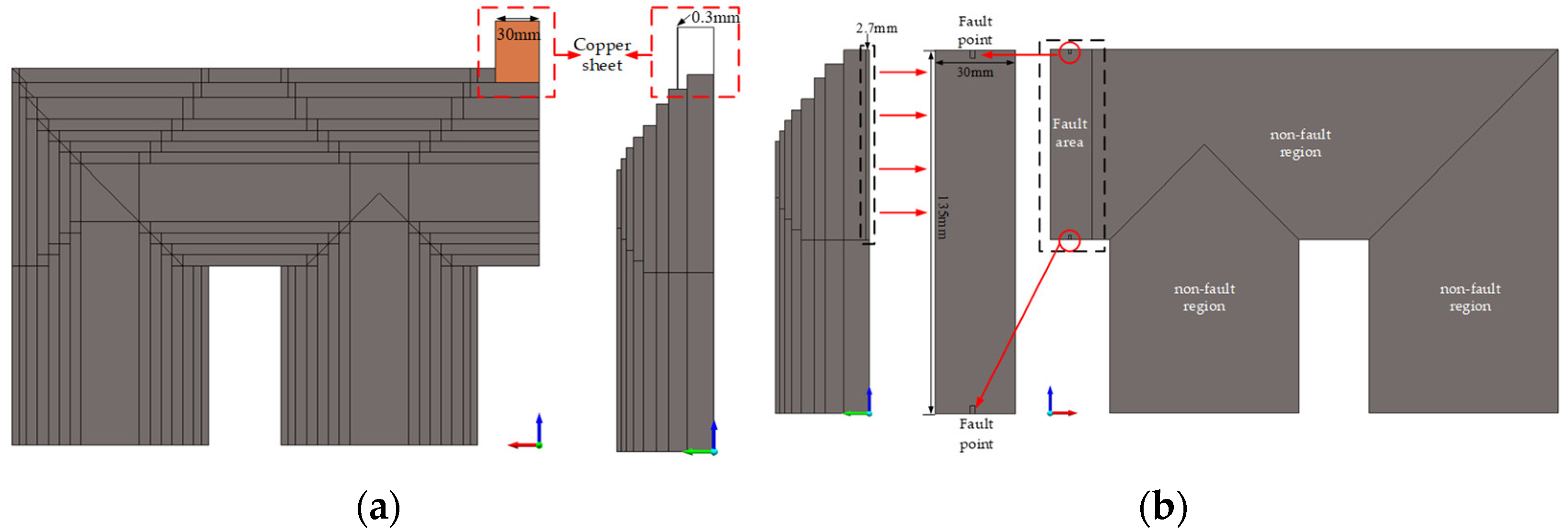
This paper is an analysis of local overheating of iron core under multi-point grounding and short circuit fault between silicon steel sheets. Multi-point grounding is divided into multi-point grounding of iron core-clamp, two-point grounding of iron core and two-point grounding of clamp. This paper is an analysis of two-point grounding fault of the iron core. The multi-point grounding faults mentioned later are also two-point grounding faults of iron core. The short circuit fault between the sheets is the overheating fault of the iron core caused by the damage of the insulating film between the silicon steel sheets and the sheets. The simulation of overheating faults under different faults needs to be completed by Magnet and Thermnet in Infolytica (7.8). The coupling mode of magneto-thermal coupling software is Magnet 7.8 time-harmonic 3D—Thermnet 7.8.3 Static 3D.

Firstly, the design of the scale model is carried out. Regardless of whether the scale is reduced or not, the Maxwell equation and constitutive relationship satisfied by the transformer are as shown in Equation (1):

$$\left\{\begin{array}{l}\nabla \cdot \dot{D}=\rho \\ \nabla \cdot \dot{B}=0\\ \nabla \times \dot{E}=-j\omega \dot{B}\\ \nabla \times \dot{H}=\dot{J}+j\omega \dot{D}\\ \dot{J}=\mathsf{\sigma }\dot{E}\\ \dot{D}=\mathsf{\epsilon }\dot{E}\\ \dot{B}=\mathsf{\mu }\dot{H}\end{array}\right.$$

(1)

where, $\dot{D}$, $\dot{B}$, $\dot{E}$, $\dot{J}$, $\dot{H}$ are electric flux density, magnetic induction intensity (magnetic flux density), electric field intensity, current density and magnetic field intensity, and they are all the effective value phasor in the eddy current field, $\omega$ is angular frequency, $\rho$, $\mathsf{\sigma }$, $\mathsf{\epsilon }$, $\mathsf{\mu }$ are charge density, conductivity, relative dielectric constant and permeability.

For the design of the scaled model, it is not only necessary to analyze the Maxwell characteristic equation, but also to analyze the winding parameters [23]. The winding parameters of the converter transformer include inductance, resistance, conductance and capacitance. The parameters affecting the loss and temperature field under the fault are the core magnetic density and the current density of the fault point. The magnetic density and current density under the fault are only affected by the resistance between the magnetic flux and the magnetic circuit of the fault point and are independent of the winding capacitance conductance parameters [9].

Therefore, only the winding resistance and inductance parameters need to be scaled, and the winding wire of the converter transformer is regarded as a long straight wire with a circular cross section. The parameters of inductance and resistance are shown in Equations (2) and (3):

$$\mathrm{L}=\frac{\mathsf{\mu }{N}^2\mathrm{A}}{l}$$

(2)

$$R=\frac{l}{\mathsf{\sigma }\mathrm{A}}$$

(3)

where L is the winding inductance value, R is the radius of the wire section, N is the number of turns of winding, A is the cross-sectional area of the wire, l is the total length of the wire and σ is the winding conductivity.

2.1.2. Similarity Theory and Similarity Relation Derivation

The scale model is based on the similarity theory. Through the characteristic equation and similarity theorem satisfied by the scale model, the similarity constant and similarity index are selected to obtain the similarity criterion, and the scale model is obtained. As described above, the scale model established in this paper is difficult to determine the similar single value condition, so the similar third theorem is used for design. The similar constants include the dielectric constant, permeability μ and conductivity σ of each component of the transformer. The similarity indexes include size, current density J, electric displacement vector D, electric field strength E and magnetic field strength H. The similarity criterion is that the magnetic flux density B is constant. Let each term in Equations (1) and (4) be equal, which is the similarity criterion of the proportional model.

According to Equation (1), the physical quantity before the scaled ratio is $\Delta$, and the physical quantity after the scaled ratio is ${\Delta }^{\prime }$, ${\Delta }^{\prime }=k_{\Delta }\Delta$, $k_{\Delta }$ is read as the scaled factor of $\Delta$, Equation (4) is the electrical characteristic equation satisfied after it is scaled, and the variant form of the Equation (4) after scaling is shown in Equation (5):

$$\left\{\begin{array}{l}{\nabla }^{\prime }\cdot {\dot{D}}^{\prime }={\rho }^{\prime }\\ {\nabla }^{\prime }\cdot {\dot{B}}^{\prime }=0\\ {\nabla }^{\prime }\times {\dot{E}}^{\prime }=-j{\omega }^{\prime }{\dot{B}}^{\prime }\\ {\nabla }^{\prime }\times {\dot{H}}^{\prime }=J^{\prime }+j{\omega }^{\prime }{\dot{D}}^{\prime }\\ {\dot{J}}^{\prime }= \mathsf{\sigma } \prime {\dot{E}}^{\prime }\\ {\dot{D}}^{\prime }= \mathsf{\epsilon } \prime {\dot{E}}^{\prime }\\ {\dot{B}}^{\prime }= \mathsf{\mu } \prime {\dot{H}}^{\prime }\end{array}\right.$$

(4)

$$\left\{\begin{array}{l}\frac{\nabla }{k}\cdot k_{\mathrm{D}}\dot{D}=k_{\mathsf{\rho }}\rho \\ \frac{\nabla }{k}\cdot k_{\mathrm{B}}\dot{B}=0\\ \frac{\nabla }{k}\times k_{\mathrm{E}}\dot{E}=-j{k}_{\mathsf{\omega }}{k}_{\mathrm{B}}\omega \dot{B}\\ \frac{\nabla }{k}\times k_{\mathrm{H}}\dot{H}=K_{\mathrm{J}}J+j{k}_{\mathsf{\omega }}{k}_{\mathrm{D}}\omega \dot{D}\\ k_{\mathrm{J}}\dot{J}=k_{\mathsf{\sigma }}{k}_{\mathrm{E}}\sigma \dot{E}\\ k_{\mathrm{D}}\dot{D}=k_{\mathsf{\epsilon }}{k}_{\mathrm{E}}\epsilon \dot{E}\\ k_{\mathrm{B}}\dot{B}=k_{\mathsf{\mu }}{k}_{\mathrm{H}}\mu \dot{H}\end{array}\right.$$

(5)

According to the similarity theory and the simplification of Equation (5), taking the known scaled coefficients such as size, magnetic flux density B, dielectric constant $\mathsf{\epsilon }$, permeability μ and conductivity σ as the basic scaled factors, the following relationship is obtained:

$$\left\{\begin{array}{l}{k}_{\mathrm{J}}=k_{\mathsf{\omega }}{k}_{\mathsf{\sigma }}{k}_{\mathrm{B}}k\\ k_{\mathrm{D}}=k_{\mathsf{\omega }}{k}_{\mathsf{\epsilon }}{k}_{\mathrm{B}}k\\ k_{\mathrm{B}}=1\\ k_{\mathrm{E}}=k_{\mathsf{\omega }}{k}_{\mathrm{B}}k\\ k_{\mathrm{H}}=k_{\mathrm{B}}/k_{\mathsf{\mu }}\end{array}\right.$$

(6)

where, k is the geometric scaled factor, $k=k_{\mathrm{x}}=k_{\mathrm{y}}=k_{\mathrm{z}}=k_{\mathrm{h}}$, $k_{\mathsf{\omega }}$ is the angular frequency scaled factor, $k_{\mathsf{\sigma }}$ is the electrical conductivity scaled factor, k_B is the magnetic flux density scaled factor, and k_μ is the magnetic permeability scaled factor.

From Equation (2), it can be seen that the inductance value is proportional to μ, the square of the numbers of turns, and the ratio of the cross-sectional area of the wire to the total length of the wire. Therefore, the variation of the inductance scaled factor is as follows:

$$k_{\mathrm{L}}=k_{\mathsf{\mu }}{k}_{\mathrm{n}}^2{k}_{\mathrm{A}/l}=1\cdot k_{\mathrm{n}}^2\cdot k_{\mathrm{A}}/k_l=1\cdot k_{\mathrm{n}}^2\cdot \mathrm{A}/{\mathrm{A}}^{\prime }\cdot N^{\prime }{l}^{\prime }/Nl$$

(7)

$$k_{\mathrm{n}}=\frac{N_1^{\prime }}{N_1}=\frac{N_2^{\prime }}{N_2}$$

(8)

where $k_{\mathrm{L}}$, $k_{\mathsf{\mu }}$, $k_{\mathrm{n}}^2$, $k_{\mathrm{A}/l}$ are the inductance value scaling coefficient, the permeability scaling coefficient, the square of the ratio of the number of turns before and after the scaling, and the ratio of the cross-sectional area of the wire before and after the scaling to the height of the winding. The permeability remains unchanged, k_μ = 1. The cross-sectional area of the conductor before and after the scale reduction of A and A’, and the total length of the conductor before and after the scale reduction of Nl and N‘l’, are 133 mm², 4.48 mm², 6822 m, 230.4 m, respectively, by calculation, and $k_{\mathrm{A}}/k_l$ is 1. N₁, N₂, $N_1^{\prime }$, $N_2^{\prime }$ are the turns of high and low voltage windings before and after scaling respectively, and the values are 1137, 568, 384, 192 respectively.

As can be seen from Equation (3), the resistance value is proportional to the reciprocal of the total length of the wire, the resistivity of the wire and the cross-sectional area of the wire, so the variation form of the scaled factor of the resistance is:

$$k_{\mathrm{R}}=\frac{k_l}{k_{\mathsf{\sigma }}{k}_{\mathrm{A}}}$$

(9)

Due to the limitation of experimental conditions, the maximum current is 30 A. Considering the experimental margin, the current on the low-voltage side is 25 A, and the current on the high-voltage side is 12.5 A. Since the capacity is 50 kVA, and the core type is single-phase four-column, the capacity on each main column is half of the total capacity of 25 kVA, so the high and low voltage winding voltages are 2 kV/1 kV, respectively. Through empirical Equation (10), the number of turns of high and low voltage windings are 384 and 192, respectively.

$$U=4.44f{B}_{m}SN$$

(10)

where, U is the transformer winding voltage, V/turn, f is 50 Hz, S is cross-sectional area of iron core column, B_m is the magnetic flux density of the core, which is 1.87 T.

2.1.3. The Establishment of Scaled Rules

In the scaled model, the magnetic flux density B is kept constant, and the length, width and radius are reduced in equal proportion to the scaled coefficient. Therefore, the scaled coefficient of the physical size is k, $k=k_{\mathrm{x}}=k_{\mathrm{y}}=k_{\mathrm{z}}=k_{\mathrm{h}}$ and k_x, k_y, k_z and k_h are the scaled factors of the iron core length, width, height and winding height, respectively. The geometric scaled parameters are shown in

Table 2. Scaled rules of geometric parameters.

Item	Master Model	Scale Model
Core column cross-sectional area	S	k2S
Core length	x	kx
Core width	y	ky
Core height	z	kz
Reactance height	h	kh

.

In the scaled model, the material is consistent, that is, permittivity $\mathsf{\epsilon }$, permeability μ and conductivity σ of the scaled model are consistent with the master model, that is, the scaled factor of these physical quantities is 1. At the same time, similar criterion magnetic flux density B remains unchanged.

In order to ensure the constant magnetic flux density, scaled factor $k_{\mathrm{B}}=1$. Due to constant material, $k_{\mathsf{\mu }}=1$, and $k_{\mathrm{B}}=k_{\mathsf{\mu }}{k}_{\mathrm{H}}$, the magnetic field intensity scaled factor $k_{\mathrm{H}}=1$. The scaling law of the electrical parameters of the scaled model can be obtained by the same reason Equations (6)–(9), as shown in

Table 3. Electrical parameters scaled rules.

Item	Master Model	Scale Model
Angular frequency	ω	ω
Resistance	R	R
Inductance	L	11.4k2L
Magnetic flux density	B	B
Magnetic field indensity	H	H
Current density	J	kJ
Electric field intensity	E	E

.

Among all the parameters in Table 3, the inductance scaling factor is not like other scaling factors and k into a power function of the relationship, because with the permeability μ, the square of the number of turns, the cross-sectional area of the wire and the total length of the wire is proportional to the ratio, so its numerical derivation process is as follows:

$$\begin{array}{l}{k}_{\mathrm{L}}=k_{\mathsf{\mu }}{k}_{\mathrm{n}}^2{k}_1\\ =1\cdot k_{\mathrm{n}}^2\cdot \frac{k_s}{k_l}=1\cdot k_{\mathrm{n}}^2\cdot \frac{S}{S^{\prime }}\cdot \frac{N^{\prime }{l}^{\prime }}{Nl}\\ =1\cdot k_{\mathrm{n}}^2\cdot \frac{1.33\times {10}^{-4}}{4.48\times {10}^{-6}}\cdot \frac{384\times 0.6}{1137\times 6}\\ =(384/1137{)}^2=(192/568{)}^2=0.114=11.4k^2\end{array}$$

(11)

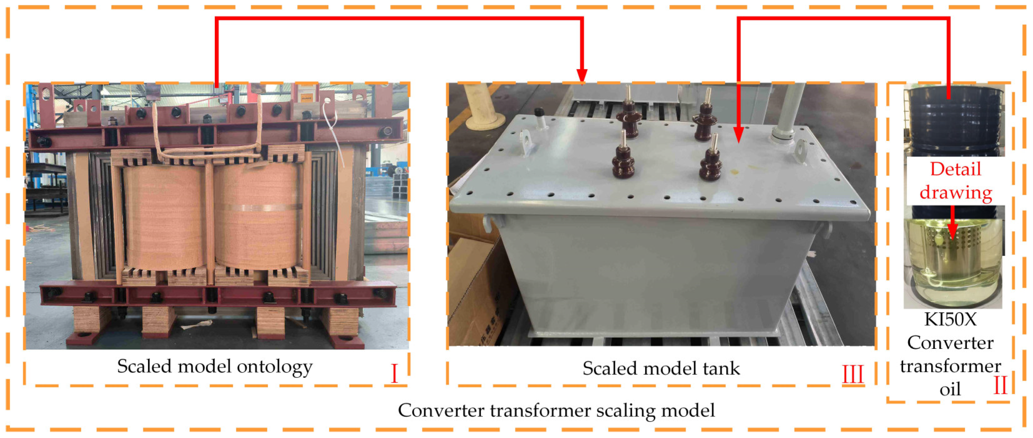
In order to analyze the temperature distribution of the scaled model on the core under fault, it is necessary to start with the loss P₀, temperature T and convective heat transfer coefficient h_T to ensure that the temperature characteristics before and after the scaling are consistent. In order to truly compare the effectiveness of temperature scaling, a scaled solid model is established in this paper, as shown in Figure 1. From the diagram, it can be seen that the scale model is composed of three parts: the body, the oil tank and the transformer oil. The body is constructed by the scale relationship. The clamps are arranged next to the upper and lower yokes to clamp the iron core. The winding is connected to the casing through the lead wire to extend out of the oil tank. The large casing is connected to the low-voltage winding, and the small casing is connected to the high-voltage winding. In order to reduce the error caused by the heat dissipation of transformer oil to the scale model, the transformer oil injected is ultra-high voltage DC transformer oil KI50X.

The above scaling process only achieves the scaling of geometric parameters and electrical parameters, and then the scaling of temperature parameters is carried out.

The steady state equation and boundary conditions of discrete finite element temperature field considering heat conduction and heat convection are shown in Equations (12)–(14):

$$\frac{\partial }{\partial x}\left({\lambda }_{\mathrm{xx}}\frac{\partial T}{\partial x}\right)+\frac{\partial }{\partial y}\left({\lambda }_{yy}\frac{\partial T}{\partial y}\right)+\frac{\partial }{\partial z}\left({\lambda }_{zz}\frac{\partial T}{\partial z}\right)=-Q_{\mathrm{V}}$$

(12)

$${\left.\frac{\partial T}{\partial n}\right|}_{\Gamma }=-\frac{1}{\left[\lambda \right]}{Q}_0$$

(13)

$${\left.-\frac{\partial T}{\partial n}\right|}_{\Gamma }=h_{\mathrm{T}}\left(T-T_{\mathrm{a}}\right)$$

(14)

where, λ_xx, λ_yy and λ_zz represent the thermal conductivity in the x, y and z directions, Q_v represents the core loss density, $\Gamma$ represents the outer boundary of the core, Q_h represents the heat flux at the boundary of the outflow core, h_T represents the convective heat transfer coefficient, T represents the core temperature, T_a represents the ambient temperature, and the ambient temperature is set at 30 °C.

Core loss is calculated by the product of the specific loss corresponding to the maximum magnetic flux density of the core and the weight of the core. The core material is unchanged, the specific loss and the core density are unchanged, that is, the p_h and ρ are unchanged. According to the Equation (15), core loss is equal to the product of additional coefficient, core weight and core specific loss, and the core weight is equal to the density multiplied by the volume, so the core loss scaling coefficient is only proportional to the volume. Because the length, width and height reduction ratio parameters of the core are all k, the core volume reduction ratio parameter is k⁻³, that is, the core loss scaling coefficient k_p is also k⁻³, as shown in Equation (16). At the same time, as 27ZH100 silicon steel sheets are used in the iron cores, thermal conductivity, constant pressure heat capacity and density are equal, and the same transformer oil is used in both of them. The oil density, thermal conductivity, constant pressure heat capacity and dynamic viscosity are consistent with the original model, and the temperature scaled parameters are shown in

Table 4. Scaled rules of temperature parameters.

Item	Master Model	Scale Model
Temperature	T	T
Core loss	P	k−3P
Core thermal conductivity	λ	λ
Core constant pressure heat capacity	Cp	Cp
Core density	ρ	ρ
Convective heat transfer coefficient	hT	k−1hT

:

$$P_0=K_{\mathrm{p}0}{p}_{\mathrm{h}}{G}_{\mathrm{Fe}}$$

(15)

where, P₀ is core loss, K_p0 is the additional coefficient of core loss, p_h is the unit loss corresponding to the maximum average magnetic flux density of the core, and G_Fe is the total weight of the core.

$$k_p=\frac{P_0^{\prime }}{P_0}=\frac{p_{\mathrm{h}}{G}_{\mathrm{Fe}}^{\prime }}{p_{\mathrm{h}}{G}_{\mathrm{Fe}}}=\frac{V_{\mathrm{Fe}}^{\prime }}{V_{\mathrm{Fe}}}=k^{-3}$$

(16)

where, k_p is core loss scaling coefficient, P^’₀ is core loss after scaling, G^’_Fe is the total weight of the core after scaling, V^’_Fe is the total volume of the core after scaling.

In order to reduce the influence of the leakage magnetic field on the temperature rise of the core under the fault of multi-point grounding and interlaminar short circuit, no-load analysis is used for the reduction model.

Therefore, the main geometric and electrical parameters of the scaled body and the scaled model are shown in

Table 5. Comparison of main parameters between scaled body and scaled model.

Item	Master Model	Scale Model
Rated capacity	412,300 kVA	50 kVA
Rated voltage	837 kV/419 kV	2 kV/1 kV
Core form	Single-phase four-column	Single-phase four-column
Core constant pressure Core diameter	1263 mm	126.3 mm
Core window height	3020 mm	302 mm

.

Through the analysis of Section 2.1, the scaling model based on the constant magnetic flux density is obtained. Next, the magnetothermal analysis of the scaled model under fault is carried out to obtain the influence of different faults on the local overheating phenomenon.

2.2. Laminate Core Homogenization Modeling and Fine Modeling

The laminated core in a converter transformer is generally modeled as a whole block, and B-H and B-P curves perpendicular to the rolling direction are assigned to the monolithic core and analyzed. However, this modeling and simulation method cannot simulate multi-point grounding and interlaminar short circuit faults, so it is necessary to use homogenization theory to simulate the two faults [15].

2.2.1. Homogenization Theory and Equivalent Electromagnetic Parameters

When the two-point grounding fault of the core occurs, a closed loop is formed between the two grounding points of the core. The closed loop intersects with the magnetic flux in the core, and the fault current will be induced. This fault current changes in the core in the same direction, spreads to all fault areas between the two fault points and passes through the insulation layer. The fault current will increase the core loss, causing local overheat points and resulting in local overheating of the core [7].

When the interlaminar short circuit fault occurs in the converter transformer scaled model, most of the interlaminar insulation in the fault area is still intact. Instead, the fault area is ablated from the fault point of the short circuit between the sheets until the insulation in the fault area is burned out or even the core is melted [10].

The anisotropy parameters proposed in literature [11] are used to simulate the scaled model electromagnetic model without fault. The equivalent permeability and equivalent conductivity are shown in Equations (17) and (18):

$$\mu =\left[\begin{array}{ccc}F{\mu }_{fx}& & \\ & {\mu }_{fy}/[F+(1-F){\mu }_{fy}/{\mu }_0]& \\ & & F{\mu }_{fz}\end{array}\right]$$

(17)

$$\sigma =\left[\begin{array}{ccc}F\sigma & & \\ & {(d/a)}^2\sigma /F& \\ & & F\sigma \end{array}\right]$$

(18)

Figure 2 shows the distribution of the main magnetic flux and eddy current of the two-dimensional infinitely long laminated core. The left figure in Figure 2 shows the vortex generated by modeling each sheet separately, and the right figure is the equivalent eddy current generated by using the homogenization parameters of Equations (17) and (18). However, the size of each lamination of the scaled model is different. According to Equation (18), σ_y is proportional to the square of the ratio of thickness to width of each lamination, that is, the eddy current generated at the first lamination is the largest, and the distribution of the generated eddy current is shown in Figure 3.

The core of the scaled model adopts 45° full oblique tertiary joints, and the core material of the core and the core material of the flow changing body are 27ZH100 silicon steel sheet. The magnetic characteristic data are measured by the magnetic characteristic test system of the project team. The permeability of x, y and z directions μ_fx, μ_fy and μ_fz are shown in Figure 4.

According to Equation (18), the conductivity perpendicular to the rolling direction changes with the thickness and width of the core stages, so the width, thickness and Y-direction conductivity of each stage are shown in

Table 6. Width, thickness and conductivity of different grades of silicon steel sheet.

Transformer Series	Width/Thickness/(mm)	${\mathit{\sigma }}_{\mathit{y}}$/(S/m)
First	135/37	8.59
Second	125/13	10.02
Third	115/8	11.84
Fourth	100/9	18.3
Fifth	85/7	26.07
Sixth	70/5	40.08
Seventh	55/3.5	69.40
Eighth	40/3	97.86

.

2.2.2. Fault Condition Modeling and Simulation Parameter Setting

In view of the eddy current loss and core temperature distribution under faults, the simulated multi-point grounding in this paper is the case that there are burrs on the core to ground the two points of the core, and the multi-point grounding mentioned in this paper is the two points of the core. The eddy current field-steady state analysis is carried out by Magnet and Thermnet in Infolytica software, that is, the core temperature distribution can be obtained.

In this paper, three forms of non-fault fault, multi-point grounding fault and interlaminar short circuit fault are considered in the simulation modeling under fault conditions. The most important consideration is the equivalent electromagnetic parameters and modeling method of the core material. The conductivity under non-fault conditions is shown in Equation (18), and the conductivity under multi-point grounding fault is shown in Equation (19) [15]

$$\sigma =\left[\begin{array}{ccc}F\sigma & & \\ & \frac{d^2\cdot \omega \cdot \mu }{2\cdot R_{\mathrm{eq}}^2\cdot b^2}& \\ & & F\sigma \end{array}\right]$$

(19)

where, R_eq is the multi-point grounding equivalent resistance, and b is the length of the silicon steel sheet.

The fault current generated by the multi-point grounding fault is induced by the magnetic flux, which forms a closed loop between the two grounding points, propagates to all fault areas between the two fault points and passes through the insulation layer, which belongs to the global fault. While the interlaminar short circuit fault is the fault point of a certain lamination, the insulation is damaged, the voltage is easily induced at the fault point, the partial discharge effect is easy to occur, and the core is ablated, which belongs to the local fault. Therefore, the fault point conductivity of interlaminar short circuit fault should be set as isotropic, and the value is the conductivity of the silicon steel sheet. The conductivity of the fault region and the non-fault region is set as shown in Equation (20) [31].

$$\sigma =\left[\begin{array}{ccc}F\sigma & & \\ & 0& \\ & & F\sigma \end{array}\right]$$

(20)

For modeling under non-fault conditions, two forms of refinement and non-refinement are considered. The so-called refinement first models the yoke, core column and side column of each level of the 50 kVA scaled model, and then stacks them together to establish an 8-layer laminated core. The overall structure is shown in Figure 5. Secondly, due to the symmetry of the model, the model is cut to one-eighth of the model, as shown in the right diagram in Figure 5. Non-refined modeling is to model the iron core as a block, without distinguishing the yoke iron, core column and side column, and without assigning equivalent electromagnetic parameters to the material.

In order to simulate a multi-point grounding fault, a copper sheet with a width of 30 mm and a thickness of 0.3 mm is inserted between the first and second stage of the upper yoke under non-fault conditions, and the copper sheet is set as a single-turn coil and the coil is short circuited to simulate two-point grounding of the core, as shown in Figure 6a. The current value in the post-treatment is the grounding current value, and the Ohmic Loss in the post-treatment is the eddy current loss generated by the core under the two-point grounding fault. In order to simulate the short circuit fault between sheets, the number of short circuit sheets is set to 10, the total thickness of the short circuit is 2.7 mm, the short circuit position is the top yoke of the core, and the short circuit fault between sheets occurs. The short circuit fault area is 135 mm in length and 30 mm in width. Therefore, the simulation model of short circuit fault between core pieces is divided into three parts: non-fault region, fault region and fault point, as shown in Figure 6b.

Since this paper only simulated the temperature field of the iron core and the temperature of the iron core did not exceed 100 °C, no-load simulation was adopted for the iron core and the heat radiation effect was ignored, and only the heat conduction inside the iron core and the heat convection between the iron core and the transformer oil were considered, and the no-load loss under the above three conditions was taken as the thermal load of the temperature field.

Because the heat convection between the transformer oil and the core meets the third type of boundary condition:

$$-\lambda {(\frac{\partial T}{\partial n})}_{\mathrm{w}}=h_{\mathrm{T}}(T_{\mathrm{w}}-T_{\mathrm{f}})$$

(21)

where λ is the thermal conductivity of the wall, unit is $\mathrm{W}/(\mathrm{m}\cdot \mathrm{K})$, T_f is the ambient temperature of transformer oil, in units of K, T_w is the temperature to be solved, in units of K, h_T is the convective heat transfer coefficient, the unit is ${\mathrm{W}/(\mathrm{m}}^2\cdot \mathrm{K})$, according to the transformer factory experience value, h_T is 2.

Table 7. Thermal properties of metallic materials.

Material	Density/(kg/m3)	$\mathbf{Heat} \mathbf{Capacity}\mathbf{/}\mathbf{(}\mathbf{J}\mathbf{/}\mathbf{(}\mathbf{kg}\cdot \mathbf{K}\mathbf{)}$)	$\mathbf{Thermal} \mathbf{Conductivity} \mathbf{(}\mathbf{W}\mathbf{/}\mathbf{(}\mathbf{m}\cdot \mathbf{K}\mathbf{)}$)
Iron core	7650	490	25
Copper sheet	8954	383.1	386
Fault area	7650	490	25

shows the thermal properties of the fault points of the iron core, multi-point ground copper and silicon steel.

3. Results and Discussion

3.1. Fine Model Analysis

By applying the rated voltage on the high voltage side, the comparison diagram of the magnetic density and eddy current loss of the refined and non-refined models is obtained, as shown in Figure 7. It can be seen from the figure that the magnetic density of the non-refined model is evenly distributed throughout the model with an average magnetic density, and the maximum magnetic density is located at the corner of the main column. It is mainly concentrated at the corner of the main column and the upper yoke, and the distribution is more uneven, showing that the closer the distance to the side column, the smaller the magnetic density distribution, which is determined by the short magnetic circuit at the corner and the magnetic anisotropy of the silicon steel sheet. The maximum excitation current calculated by fine and non-fine simulation is 0.02178 A and 0.019 A, the design value is 0.021 A, and the error is 3.7% and −9.5%, indicating that the magnetic flux simulated by two models are similar to the theoretical design value.

Figure 7c,d shows the distribution of eddy current loss in the non-refined and refined models. Eddy current is mainly distributed at the corner of the core column and the yoke, because the magnetic density change at this corner is large and more eddy current is generated. In the refined model, with the increase of lamination series, the magnetic density of the corner gradually decreases, the eddy current decreases, and the eddy current loss decreases accordingly, showing the eddy current loss distribution.

Post-processing results show that eddy current loss under non-fault conditions is 62.08 W. Because the main magnetic flux is uniform, and the thickness of a single lamination is 0.3 mm, the width of the rolling direction is 40 mm, and the length perpendicular to the rolling direction is 100 mm. 0.3 mm is much smaller than 40 mm and 100 mm, which means that 0.3 mm is smaller than the width of the rolling direction and the length perpendicular to the rolling direction under all stages. According to the literature [11], the model established in this paper satisfies two assumptions:

(1)

The thickness of a single lamination is much smaller than the width of the rolling direction and the length perpendicular to the rolling direction.

(2)

Uniform main magnetic flux.

Therefore, the eddy current loss can be verified by one-dimensional calculation formula, as shown in Equation (22):

$$\frac{P_e}{V}=\frac{\sigma {\omega }^2{d}^2{B}_m^2}{8}\frac{1}{{\xi }_2}\frac{\sinh {\xi }_2-\sin {\xi }_2}{\cosh {\xi }_2-\cos {\xi }_2}({\mathrm{W}/\mathrm{m}}^3)$$

(22)

where, ${\xi }_2$ is skin effect factor, ${\xi }_2=d/\sqrt{\frac{2}{\omega {\mu }_{\mathrm{fz}}\sigma }}$.

The results show that the eddy current loss under non-fault conditions is 66.60 W and the error is 6.78%, which verifies the accuracy of the eddy current loss calculated by the homogenization model.

In

Table 8. Comparison of eddy current loss between non-refined model and refined model.

Material	Eddy Current Loss (W)	Error (%)
Non-fine model	47.48	28.71%
Fine model	62.08	6.78%
Analytical method	66.60	-

, the eddy current loss of the non-refined model is compared with that of the refined model. The eddy current loss error of the refined model is 6.78%, while that of the non-refined model is 28.71%, which indicates that the simulation of laminated core failure under the refined model is more accurate.

3.2. Electrical Thermal Analysis of Fault Conditions

The magnetic density, eddy current, loss and temperature of multi-point grounding fault and interlaminar short circuit fault under fine modeling are analyzed respectively.

3.2.1. Multi-Point Grounding Fault Electrical Analysis

Figure 8 shows the magnetic density and eddy current distribution of the multi-point grounding fault, respectively. The multi-point grounding position is located in the upper yoke of the first and second stage of the lamination, and the ground fault current generated will flow in and out along the direction of the silicon steel sheet lamination. It can be seen from the figure that the maximum magnetic density of the iron core reaches 2.00 T, and the maximum position appears at the corner of the second and third lamination. Because the multi-point grounding is a global fault, it is not a fault for a certain point or a certain position, and the magnetic density here is small due to the magnetic anisotropy and magnetic circuit length, and the eddy current induced here is small.

Figure 8 shows the eddy current loss distribution of the multi-point grounding fault. However, the fault current induced by the -Z side of the first and second levels of the upper yoke (the position connected to the main column) is very large. As shown in Figure 8b, the maximum fault current density occurs between the first and second levels of the stack, and the maximum value reaches 1.21 × 10⁵ A/m². Because eddy current loss is the loss caused by eddy current forming a path in the silicon steel sheet, the distribution of eddy current loss should be basically consistent with the distribution of fault current density. As shown in Figure 9, the eddy current loss density distribution in the second-stage stack is radially diffused outward and reaches its maximum in the center of the second-stage stack, whose value is 1.29 × 10⁵ W/m³. From the fault current distribution in Figure 8b, it can be seen that the fault current passing along the laminate direction gathers at the edges on both sides of the laminate, distributes evenly on the first-and-second-tier laminate boundary (insulation boundary), and converges to the edges on both sides of the laminate along the Y direction after passing through the boundary.

3.2.2. Interlaminar Short Circuit Fault Electrical Analysis

Figure 10 and Figure 11 shows the distribution of magnetic density, eddy current and eddy current loss under interlaminar short circuit fault. It can be seen from the figure that the distribution of magnetic density under interlaminar short circuit fault is similar to that under non-fault fault, indicating that interlaminar short circuit fault is a local fault and does not affect the overall magnetic density distribution. The maximum eddy current at the fault point reaches 2.76 × 10⁵ A/m², which is much higher than the eddy current at the same position under non-fault conditions, which is prone to partial discharge effect. The eddy current at the upper fault point is at a very low value, which is analyzed because the magnetic density at this position is very small. Even if the conductivity at the fault point is different from [σ] under non-fault conditions, but has isotropic conductivity, it still indicates that the eddy current induced is very small.

As can be seen from

Table 9. Analysis of electrical characteristics under fault.

Fault	Maximum Eddy Current Density (A/m2)	Eddy Current Loss (W)	Iron Loss (W)
Non-fault	104,360	7.76	14.17
Multi-point grounding	121,026	8.84	16.14
Interlaminar short circuit	275,628	7.79	14.23

, the eddy current loss of 1/8 model under non-fault condition is 7.76 W, the eddy current loss under multi-point grounding fault reaches 8.84 W with a loss increment of 13.90%, and the eddy current loss under interlaminar short circuit fault reaches 7.79 W with a loss increment of 0.42%. Accordingly, the increment of iron loss under the two faults is consistent with that of eddy current loss, which is also 13.90% and 0.42%. These increased losses will be introduced into the thermal field as a heat source for simulation.

Observing the change of the maximum current density, it is found that the maximum current density of the multi-point grounding is 1.16 times that of the fault-free, while the maximum current density of the interlaminar short circuit fault point is 2.64 times. In comparison, the interlaminar short circuit fault is more prone to partial discharge ablation of the core and local overheating. The multi-point grounding fault is not prone to partial discharge but is more likely to increase the overall temperature of the core.

3.2.3. Fine Modeling Thermal Analysis of Different Faults

As can be seen from Figure 12, the difference in core temperature between the non-refined model and the refined model is the same temperature distribution, but the refined core temperature is higher than that of the non-refined model, the maximum temperature increases from 53.68 $°\mathrm{C}$ to 55.10 $°\mathrm{C}$, and the calculation accuracy increases by 2.58%. It can be seen that the refined model can achieve more accurate results.

Figure 13 shows the cloud diagram of core temperature under multi-point grounding fault and interlaminar short circuit fault. It can be seen from the diagram that the temperature on the main column under multi-point grounding is the highest, with an average value of 57.85 °C. The temperature of the fault point in the inter-plate short circuit reaches 53.40 °C. Comparing the three figures, it can be seen that the multi-point grounding is a global fault, which affects the overall temperature maximum value and increases the average temperature of the main column, side column and upper yoke of the core. The interlaminar short circuit is a local fault, which basically does not affect the overall temperature maximum value, but only affects the temperature distribution at the fault point.

Table 10. Thermal characteristic analysis under fault.

Fault	Maximum Iron Core Temperature (°C)	Temperature Increase (%)
Non-fault	55.10	-
Multi-point grounding	58.20	5.63
Interlaminar short circuit	55.80	1.27

shows the influence of different faults on the maximum core temperature of the transformer. Under non-fault conditions, the maximum core temperature occurs at the corner of the core main column, and its value is 55.10 °C. Under multi-point ground fault and interlaminar short circuit fault, the maximum core temperature is 58.20 °C and 55.80 °C respectively, and the temperature increase is 5.63% and 1.27% respectively.

As shown in Figure 13, the midpoint of the upper fault point is set as point A, and the lower fault point is set as point B. The temperature distribution along the path under the three working conditions is shown in Figure 14. It can be seen from the figure that under the same position, the temperature of the upper fault point and the lower fault point of the interlaminar short circuit is 0.08 °C and 0.1 °C higher than that under the non-fault condition, respectively, while that of the multi-point grounding fault is 2.89 °C and 3.27 °C higher. This shows that the multi-point grounding fault is more serious to the local overheating problem of the transformer. If the multi-point grounding crosses more stages, the more the magnetic flux of the cross-link, the greater the loss will be, and the higher the temperature will be generated on the core. Interlaminar short circuit is a burr phenomenon on the simulated silicon steel sheet. Usually, only two very small fault points have interlaminar short circuit. If the burr increases and occurs in the UHV converter transformer, the loss and temperature rise caused are immeasurable and the harm is also huge.

4. Conclusions

In order to improve the calculation accuracy of magnetic density, eddy current density and eddy current loss of the transformer core, a refined modeling method is proposed in this paper. Considering the cost and experimental conditions of the fault experiment of the converter transformer, this paper designs a scaled model of the converter transformer to facilitate the subsequent experimental work.

Firstly, based on the scaling principle of constant magnetic flux density, the scaling model of the converter transformer is established. Secondly, based on the refined modeling method and the non-refined modeling method, the core magnetic density, eddy current loss and core temperature of the scaled model are simulated and analyzed respectively, and the eddy current loss is verified by the one-dimensional eddy current loss analytical equation. Thirdly, the homogenization theory and FEM are used to numerically study the refined modeling method of the scaled model under multi-point grounding and interlaminar short circuit faults. The main conclusions are as follows:

The error between the eddy current loss based on the non-refined model and the analytical calculation eddy current loss is 28.71%, while the error between the eddy current loss based on the refined model and the analytical calculation eddy current loss is 6.78%, and the calculation accuracy is improved by 21.93%.

The multi-point grounding fault simulation results based on the refined model show that when the multi-point grounding crosses the first-stage lamination of the core, the overall temperature increases by 3 °C, indicating that the multi-point grounding is a global overheating effect, but the current density change effect is not significant. The simulation results of the interlaminar short circuit fault based on the refined model show that the current temperature of the fault point is increased by 0.12 °C, but the hottest spot is still located in the core column, indicating that the interlaminar short circuit is a local overheating effect. At the same time, the current density of the fault point reaches 2.64 times of the non-fault, and the current density change effect is significant, which is prone to suspension discharge effect.

In this paper, the initial temperature of multi-point grounding and interlaminar short circuit fault is given, which provides a basis for the future research on the influence of temperature after ablation of fault location on local overheating problem in a period of time after two overheating faults.

References

1. Dragan, J. HVDC Rectifier Station Modelling, Control and Synchronisation with AC System. In High Voltage Direct Current Transmission; John Wiley & Sons, Ltd.: Hoboken, NJ, USA, 2019; pp. 37–41. [Google Scholar]
2. Feng, J.; Yu, G.; Zhao, M.; Zhang, J.; Lu, S. Dynamic Risk Assessment Framework for Industrial Systems Based on Accidents Chain Theory: The Case Study of Fire and Explosion Risk of UHV Converter Transformer. Reliab. Eng. Syst. Saf. 2022, 228, 108760. [Google Scholar] [CrossRef]
3. Jiang, P.; Zhang, Z.; Dong, Z.; Wu, Y.; Xiao, R.; Deng, J.; Pan, Z. Research on Distribution Characteristics of Vibration Signals of ±500 kV HVDC Converter Transformer Winding Based on Load Test. Int. J. Electr. Power Energy Syst. 2021, 132, 107200. [Google Scholar] [CrossRef]
4. Li, Y.; Yan, X.; Zhang, C.; Chen, Y.; Ying, W. Numerical prediction of losses and local overheating in transformer windings based on magnetic-thermal-fluid model. Trans. China Electrotech. Soc. 2020, 35, 4483–4491. [Google Scholar]
5. Li, B.; Wang, Z.; Liu, H.; Li, H.; Liu, J. Experiment on vibro-acoustic characteristic of 500 kV single-phase transformer under DC-bias. Trans. China Electrotech. Soc. 2021, 36, 2801–2811. [Google Scholar]
6. Liu, J.; Meng, D.; Xia, Y.; Ai, M. Simulation study of interlamination short circuit fault in cores based on homogenization theory. Electr. Mach. Control. 2020, 24, 1–8. [Google Scholar]
7. Zhou, L.; Liu, H.; Gao, S.; Jiang, J.; Li, W.; Guo, L. A homogenization modeling method of transformer cores considering multipoint grounding faults. Proc. CSEE 2018, 38, 3709–3716+31. [Google Scholar]
8. Zhou, L.; Liu, H.; Gao, S.; Jiang, J.; Wang, D.; Zhang, J. Three-dimensional modeling and analysis of eddy current field of transformer core during short circuit between sheet. J. China Railw. Soc. 2018, 40, 33–39. [Google Scholar]
9. Zhou, X.; Luo, Y.; Tian, T.; Bai, H.; Wu, P.; Liu, W. Transformer Fault Diagnosis Based on Probabilistic Neural Networks Combined with Vibration and Noise Characteristics. Front. Energy Res. 2023, 11, 1169508. [Google Scholar] [CrossRef]
10. Wang, J.; Lin, H.; Huang, Y.; Huang, L. Numerical Analysis of 3D Eddy Current Fields in Laminated Media Under Various Frequencies. IEEE Trans. Magn. 2012, 48, 267–270. [Google Scholar] [CrossRef]
11. Geri, A.; Salvini, A.; Veca, G.M. Displacement Eddy Current Computation in Magnetic Laminates. IEEE Trans. Magn. 1994, 30, 1075–1077. [Google Scholar] [CrossRef]
12. Loisos, G.; Moses, A.J.; Beckley, P. Electrical Stress on Electrical Steel Coatings. J. Magn. Magn. Mater. 2003, 254–255, 340–342. [Google Scholar] [CrossRef]
13. Hamzehbahmani, H.; Anderson, P.; Hall, J.; Fox, D. Eddy Current Loss Estimation of Edge Burr-Affected Magnetic Laminations Based on Equivalent Electrical Network—Part II: Analytical Modeling and Experimental Results. IEEE Trans. Power Deliv. 2014, 29, 651–659. [Google Scholar] [CrossRef]
14. Pu, Z.-H.; Ruan, J.-J.; Du, Z.-Y.; Zhang, Y.-D.; Li, J.-L.; Xie, Q.-J.; Tan, D. Analysis of Voltage Distribution Characteristics in UHVDC Converter Transformer Winding Based on the Reduced-Scale Model. IEEE Trans. Magn. 2014, 50, 1–5. [Google Scholar] [CrossRef]
15. Preis, K.; Biro, O.; Ticar, I. FEM Analysis of Eddy Current Losses in Nonlinear Laminated Iron Cores. IEEE Trans. Magn. 2005, 41, 1412–1415. [Google Scholar] [CrossRef]
16. Bermudez, A.; Gomez, D.; Salgado, P. Eddy-Current Losses in Laminated Cores and the Computation of an Equivalent Conductivity. IEEE Trans. Magn. 2008, 44, 4730–4738. [Google Scholar] [CrossRef]
17. Wang, J.; Lin, H.; Huang, Y.; Sun, X. A New Formulation of Anisotropic Equivalent Conductivity in Laminations. IEEE Trans. Magn. 2011, 47, 1378–1381. [Google Scholar] [CrossRef]
18. Kaimori, H.; Kameari, A.; Fujiwara, K. FEM Computation of Magnetic Field and Iron Loss in Laminated Iron Core Using Homogenization Method. IEEE Trans. Magn. 2007, 43, 1405–1408. [Google Scholar] [CrossRef]
19. Hamzehbahmani, H.; Anderson, P.; Eldieb, A. An Overview of the Recent Developments of the Inter-Laminar Short Circuit Fault Detection Methods in Magnetic Cores. In Proceedings of the 50th International Universities Power Engineering Conference, UPEC 2015, Stoke-on-Trent, UK, 1–4 September 2015. [Google Scholar]
20. Altayef, E.; Anayi, F.; Packianather, M. Power Transformer Fault Detection Methods and Effects of Edge Burrs Fault: A Review. In Proceedings of the 2nd International Conference on Advance Computing and Innovative Technologies in Engineering, ICACITE 2022, Greater Noida, India, 28–29 April 2022. [Google Scholar]
21. Hamzehbahmani, H.; Anderson, P.; Jenkins, K. Interlaminar Insulation Faults Detection and Quality Assessment of Magnetic Cores Using Flux Injection Probe. IEEE Trans. Power Deliv. 2015, 30, 2205–2214. [Google Scholar] [CrossRef]
22. Altayef, E.; Anayi, F.; Packianather, M.S.; Kherif, O. On the Effects of Lamination Artificial Faults in a 15 kVA Three-Phase Transformer Core. IEEE Access 2022, 10, 19348–19355. [Google Scholar] [CrossRef]
23. Hernandez-Robles, I.A.; Olivares-Galvan, J.C.; Lopez-Garcia, I.; Hernandez-Avila, J.L.; Escarela-Perez, R.; Magdaleno-Adame, S. Experimental and Numerical Analysis of Shorted Interlaminations in Transformer Cores. In Proceedings of the 2016 IEEE PES Transmission and Distribution Conference and Exposition-Latin America, PES T and D-LA 2016, Morelia, Mexico, 20–24 September 2016. [Google Scholar]
24. Wang, Z.; Dai, Y.; Wang, B.; Sun, T. Refined Thermal Analysis and Electrical Strength Check of Natural Ester Transformer. High Volt. 2021, 47, 742–751. [Google Scholar]
25. Xiao, F.; Zhang, X.; Wang, R.; Ren, Q. A Detailed Thermal Network Modeling Method of Water-cooled Epoxy-cast Transformer Windings With Double-wing Finned Tubes. Proc. CSEE 2022, 42, 8321–8332. [Google Scholar]
26. Zhao, X.; Zhang, J.; Wang, H.; Miao, Y.; Liu, L. A refined simulation method for the vibration characteristics of transformer core considering the influence of air gap under the perspective of electro-magnetic-mechanical coupling. Trans. China Electrotech. Soc. 2023, 1–12. [Google Scholar]
27. Zakrzewski, K.; Tomczuk, B.; Waindok, A. Nonlinear scaled models in 3D calculation of transformer magnetic circuits. COMPEL Int. J. Comput. Math. Electr. Electron. Eng. 2006, 25, 91–101. [Google Scholar] [CrossRef]
28. Willem, G.O.; Jan, A.F. Effects of scaling high-frequency transformer parameters. IEEE Trans. Ind. Appl. 1999, 35, 932–940. [Google Scholar]
29. Yang, Q.; Chen, Y.; Sima, W.; Zhao, H.; Liu, H. Winding impulse voltage distribution based on transformer reduced-scale mode. High Volt. 2016, 42, 3955–3963. [Google Scholar]
30. Zou, L.; Gong, P.; Zhang, L.; Zhao, T.; Li, Q. Small-scale experiment and model simplification of space magnetic fields around air-core reactors. High Volt. 2014, 40, 1675–1682. [Google Scholar]
31. Wang, J.; Lin, H.; Fang, S.; Huang, Y. Validity and accuracy of eddy current field analysis of laminations by introducing equivalent conductivities. Proc. CSEE 2012, 32, 162–168+197. [Google Scholar]
Figure 1. Converter transformer scaled model.
Energies 17 01047 g001
Figure 2. The main flux and eddy current of two dimensional infinitely long laminated core. Where, d is the thickness of a single laminated sheet, b is the thickness of one grade, and a is the width of the iron core, and H ˙ 0 is the direction of the main magnetic flux, F is the core lamination coefficient, value is 0.96.
Energies 17 01047 g002
Figure 3. Physical lamination size and eddy current distribution. Where, d1d8 is the thickness of each stack, a1a8 is the width of each stack, and H ˙ 0 is the direction of the main magnetic flux.
Energies 17 01047 g003
Figure 4. 27ZH100 silicon steel sheet permeability.
Energies 17 01047 g004
Figure 5. Finite element model under non-fault. Where, ξ1 and ξ2 are ideal magnetic conductor boundaries, and the XOZ plane on the -Y side of one-eighth is the magnetic insulation boundary. The red H0 represents the magnetic field strength, the orange arrow represents the flow direction of the magnetic field strength, and the green represents the different positions of the iron core.
Energies 17 01047 g005
Figure 6. Finite element model of multi-point grounding and interlaminar short circuit fault. (a) Multi-point grounding model. (b) Interchip short circuit model.
Energies 17 01047 g006
Figure 7. Contrast between fine modeling and non-fine modeling. (a) Non-fine magnetic density. (b) Fine magnetic density. (c) Non-fine eddy current loss. (d) Fine eddy current loss.
Energies 17 01047 g007aEnergies 17 01047 g007b
Figure 8. Magnetic density and eddy current under multi-point grounding fault condition. (a) Magnetic density distribution. (b) Eddy density distribution.
Energies 17 01047 g008
Figure 9. Magnetic density and eddy current under multi-point grounding fault condition.
Energies 17 01047 g009
Figure 10. Magnetic density and eddy current under interlaminar short circuit fault condition. (a) Magnetic density distribution. (b) Eddy density distribution.
Energies 17 01047 g010
Figure 11. Eddy current loss under interlaminar short circuit fault condition.
Energies 17 01047 g011
Figure 12. Temperature contrast between fine modeling and non-fine modeling. (a) Non-fine temperature distribution. (b) Fine temperature distribution.
Energies 17 01047 g012
Figure 13. Temperature distribution under faults. (a) Multi-point grounding temperature. (b) Interlaminar short circuit temperature.
Energies 17 01047 g013
Figure 14. Temperature distribution between AB paths under different faults.
Energies 17 01047 g014