Feature Extraction of Flow Sediment Content of Hydropower Unit Based on Voiceprint Signal

Abstract

The hydropower turbine parts running in the sand-bearing flow will experience surface wear, leading to a decline in the hydropower unit’s stability, mechanical performance, and efficiency. A voiceprint signal-based method is proposed for extracting the flow sediment content feature of the hydropower unit. Firstly, the operating voiceprint information of the hydropower unit is obtained, and the signal is decomposed by the Ensemble Empirical Mode Decomposition (EEMD) algorithm, and a series of intrinsic mode functions (IMFs) are obtained. Combined with correlation analysis, more sensitive IMF components are extracted and input into a convolutional neural network (CNN) for training, and the multi-dimensional output of the fully connected layer of CNN is used as the feature vector. The k-means clustering algorithm is used to calculate the eigenvector clustering center of the hydropower unit with a clean flow state and a high sediment content state, and the characteristic index of the hydropower unit sediment content is constructed based on the Euclidean distance method. We define this characteristic index as SI, and the change in the SI value can reflect the degree of sediment content in the flow of the unit. A higher SI value indicates a lower sediment content, while a lower SI value suggests a higher sediment content. Combined with the sediment voiceprint data of the test bench, when the water flow changed from clear water to high sediment flow (1.492 × 10⁵ mg/L), the SI value decreased from 1 to 0.06, and when the water flow with high sediment content returned to clear water, the SI value returned to 1. The experiment proves the effectiveness of the method. The extracted feature index can be used to detect the flow sediment content of the hydropower unit and give early warning in time, so as to improve the maintenance level of the hydropower unit.

1. Introduction

The development of impulse turbines adapted to high-head hydropower energy has broad market prospects [1]. In the process of power generation for an impulse turbine, the runner is driven by a high-speed jet to do work, and the sand particles in the water flow with high sediment content will cause the wear problem of turbine parts [2]. It will cause material erosion of hydraulic flow parts and a decline in efficiency, aggravate vibration and fatigue damage, and threaten the safe and stable operation of the unit.

Erosion wear of an impact turbine runner is a complex phenomenon that is related to sediment particle size, hardness and concentration, water flow velocity, substrate performance, and other parameters [3,4]. Compared with particle diameter, sediment concentration can more affect the output of the bucket and runner, thus affecting the overall efficiency of the turbine. The maximum wear of the runner is positively correlated with sediment concentration. The higher the concentration, the more prominent the surface wear and the larger the wear area [5,6]. Therefore, a detection method that can reflect the sediment content of the unit flow in real time is needed. When the sediment content of the unit flow is serious, the unit operation status can be adjusted or shut down actively so as to avoid the harm caused by high sediment content flow to the unit, which is of great significance for improving the maintenance level of the unit state, curbing the spread of faults, and reducing the loss of faults.

The running voiceprint signal of a hydropower unit contains a large amount of effective information reflecting the internal mechanical state of the equipment, which is characterized by nonlinear and non-stationary characteristics and is a compound noise with random process characteristics [7]. When the state of the equipment changes, the voiceprint signal generated by its state will also change accordingly [8]. Moreover, voiceprint signals have the characteristics of non-contact, easy measurement, and higher freedom of sensor installation. Therefore, equipment status recognition technology based on voiceprint signals has been widely used and has achieved good results. For example, Tang et al. [9] used voiceprint signal analysis method and combined with actual cases to carry out fault analysis and diagnosis of hydropower units; Ni et al. [10] proposed a ship radiated noise recognition method based on Variational Mode Decomposition (VMD) and improved Convolutional Neural Networks (CNN) to accurately identify target ships; Zhou et al. [11] found that the acoustic emission signal frequency distribution characteristics showed obvious differences in different working states of the tool head, and based on this, the running state of the tool could be accurately judged; Weng et al. [12] accurately identified the friction state of liquid film seals based on time-frequency analysis of acoustic emission signals and convolutional neural network system. The research shows that voiceprint analysis is an effective method to study the fault characteristics and state evaluation of equipment. However, at present, the application of voiceprint analysis technology to the extraction of sediment content features from hydropower units has not been reported.

In signal processing, Ensemble Empirical Mode Decomposition (EEMD), developed on the basis of Empirical Mode Decomposition (EMD), has been widely used in non-stationary signal analysis because end effects and mode aliasing are suppressed [13,14].

Deep learning algorithms have powerful capabilities in data processing and information mining [15]. The latest research shows that CNN can achieve deep potential feature information mining through a large number of sample trainings [16,17]. The application of CNN to the field of voiceprint has achieved certain results [18,19].

Therefore, a feature extraction method for the flow sediment content of hydropower units based on a voiceprint signal is proposed. It takes the hydropower unit voiceprint signal as the premise, based on the advantages of EEMD in non-stationary signal analysis, the characteristics of suppressing end effects, mode aliasing, and the advantages of CNN in mining deep potential feature information. In this method, the collected voiceprint data was first decomposed by EEMD, several intrinsic mode functions (IMF) were extracted, and correlation analysis was performed to retain the features sensitive to the unit operating state. CNN is input to complete the training and extract the feature vector of the fully connected layer. Finally, the characteristics of the flow sediment concentration of the hydropower unit were constructed by combining the clustering algorithm and Euclidian distance. The effectiveness of the proposed method was verified by combining it with the acoustic print data of the experimental platform.

2. Materials and Methods

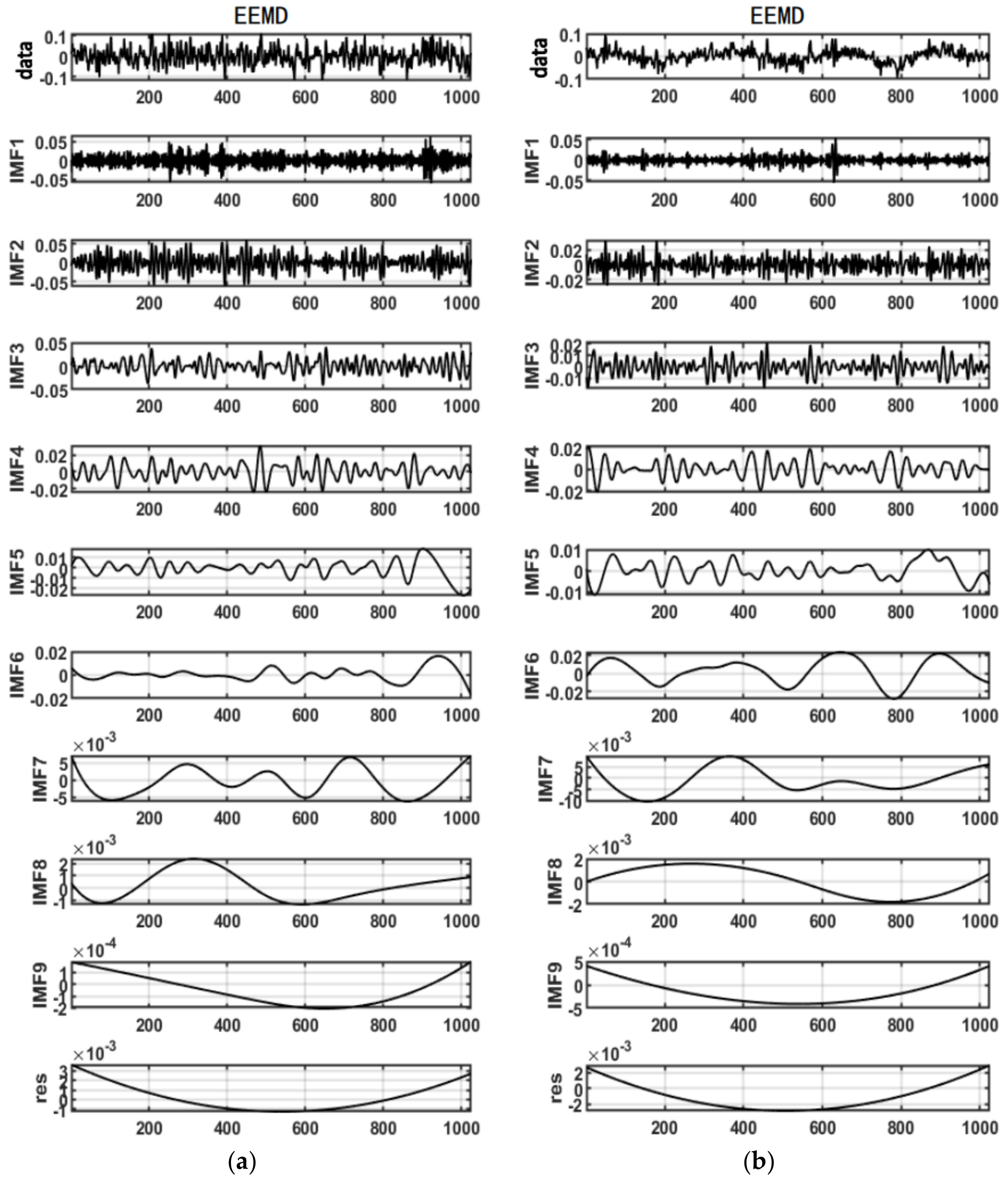
2.1. Ensemble Empirical Mode Decomposition

The Ensemble Empirical Mode Decomposition (EEMD) method was proposed by Huang et al. It changes the extreme point characteristics of the signal by adding white noise each time and then performs the overall average of multiple intrinsic mode functions (IMFs) obtained from the EMD to offset the added white noise, thus effectively suppressing mode aliasing [13]. The total number of noises added is N, and the steps of EEMD are as follows:

(1) A standard normal distribution of white noise $n_i\left(t\right)$ is added to the original signal $x\left(t\right)$:

$$x_i\left(t\right)=x\left(t\right)+n_i\left(t\right)$$

(1)

where $n_i\left(t\right)$ represents the added white Gaussian noise, i is the added sequence, $x_i\left(t\right)$ is the signal data after the addition of white Gaussian noise, and $i$ is the signal data sequence.

(2) The signal in Formula (1) is decomposed by EMD to obtain $j$ modal components and a residual component:

$$x_i\left(t\right)={\displaystyle \sum }_{j=1}^{J}IM{F^{\prime }}_j+e_i\left(t\right)$$

(2)

where $IM{F^{\prime }}_j$ is the $j$ modal component and a residual component of $x_i\left(t\right)$ generated by EMD, and $e_i\left(t\right)$ is the average trend of the signal.

When the j-order residual component becomes a monotone function and can no longer screen out the IMF component, the screening is stopped, and $j$ is the number of selected modal components.

(3) Steps (1) and (2) are repeated N times to obtain the IMF set, as follows:

$$\left\{c_{1,j}\left(t\right),c_{2,j}\left(t\right),\dots ,c_{N,j}\left(t\right)\right\}, j=1,2,\dots ,J$$

(3)

(4) Aggregate average the obtained IMF to obtain the final component of EEMD [20]:

$$c_j\left(t\right)=\frac{1}{N}{\displaystyle \sum }_{i=1}^N{c}_{i,j}\left(t\right)$$

(4)

where $c_j\left(t\right)$ is the jth IMF obtained by EEMD decomposition.

According to the literature [14], this study adopts $Nstd=0.2$ and $NE=100$ as parameters of EEMD signal decomposition; $Nstd$ is the ratio of the standard deviation of additional noise to the standard deviation of the original signal; and $NE$ is the average number of times of the signal.

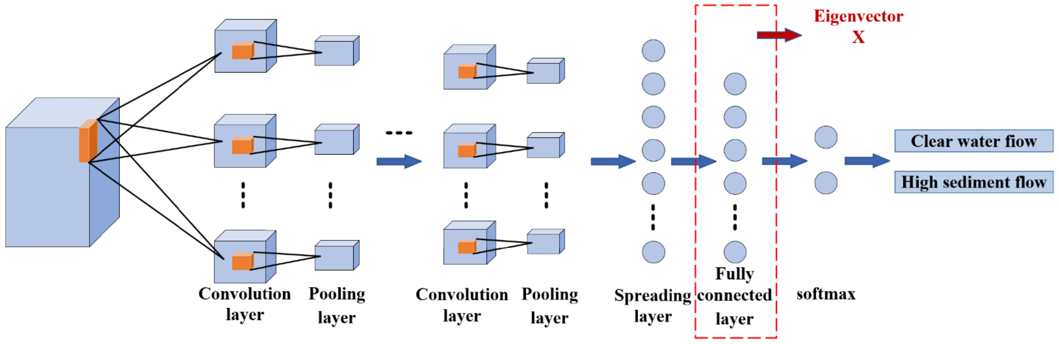
2.2. Convolutional Neural Networks

CNN is a feedforward neural network with convolutional computation and a deep neural network structure [21]. The main structure is an input layer, a hidden layer, a fully connected layer, and an output layer. The hidden layer includes a convolutional layer, an activation layer, and a pooling layer [22,23]. The common convolutional neural network structure is shown in Figure 1.

Convolution layer: The feature extraction of input data is realized through convolution operations to obtain different representation features of the input data, which is the key to characterizing CNN learning ability [24].

Activation layer: the transfer function is generally an S-type activation function $f\left(x\right)=\frac{1}{1+e^{-x}}$, but it is prone to gradient disappearance. This study proposes that the Rectified Linear Unit (ReLU) activation function be used in the model, which can effectively avoid gradient disappearance in the training process [16]. The mathematical expression of the ReLU activation function is as follows:

$$f\left(x\right)=\left\{\begin{array}{c}x,x>0\\ 0,x\le 0\end{array}=\max \left(0,x\right)\right.$$

(5)

Pooling layer: Through pooling operations, this layer retains useful information, eliminates redundant parameters and features, and reduces the resolution of the feature surface.

Fully connected layer: This layer is the connection layer between the main structure of the convolutional neural network and the output results. It is connected with all the neurons of the last pool layer, and the output features are connected end to end to form a one-dimensional feature vector, which is passed to the classifier to complete the classification.

In this study, we chose the Softmax classifier to output the results of CNN. The Softmax classifier is the most commonly used result output function in CNN. This function can reduce the training difficulty and make the convergence of multi-classification problems easier [25]. Its mathematical expression is as follows:

$$f\left(z^i\right)=\frac{e^{z^i}}{{{\displaystyle \sum }}_{\mathrm{K}}^{\mathrm{M}}{e}^{z^{\mathrm{k}}}}$$

(6)

where $z^i$ is the fractional value of the $i$ nerve, and $M$ is the classification species.

2.3. K-Means Clustering Algorithm

Clustering is to divide the samples into several categories through the internal relationship between the data without knowing any sample labels in advance, so that the similarity between the samples of the same category is high and the similarity between the samples of different categories is low, and the clustering center of each category is solved. Specific implementation steps are as follows:

(1) Data preprocessing. Mainly standardized, outlier filtering.

(2) K centers were randomly selected and denoted as ${\mu }_1^{\left(0\right)},{\mu }_2^{\left(0\right)},\dots ,{\mu }_k^{\left(0\right)}$.

(3) The loss function is defined as follows:

$$J\left(c,\mu \right)=min{{\displaystyle \sum }}_{i=1}^M{\left|\left|x_i-{\mu }_{ci}\right|\right|}^2$$

(7)

(4) Let t = 0, 1, 2, ... This is the number of iterative steps. The following process is repeated until $J$ converges:

Each sample $x_i$ is assigned to the nearest center:

$$c_i^t<-argmi{n}_k{\left|\left|x_i-{\mu }_k^t\right|\right|}^2$$

(8)

For each cluster center $k$, the center of the cluster is recalculated:

$${\mu }_k^{\left(t+1\right)}<-argmi{n}_{\mu }{{\displaystyle \sum }}_{i:c_i^t=k}^b{\left|\left|x_i-{\mu }_k^t\right|\right|}^2$$

(9)

First, the center point is fixed, and the category of each sample is adjusted to reduce $J$. Then, the category of each sample is fixed, the center point is adjusted, and $J$ is reduced. The two processes cycle alternately: $J$ monotonically decreases until the minimum, and the center point and the class of the sample partition converge simultaneously.

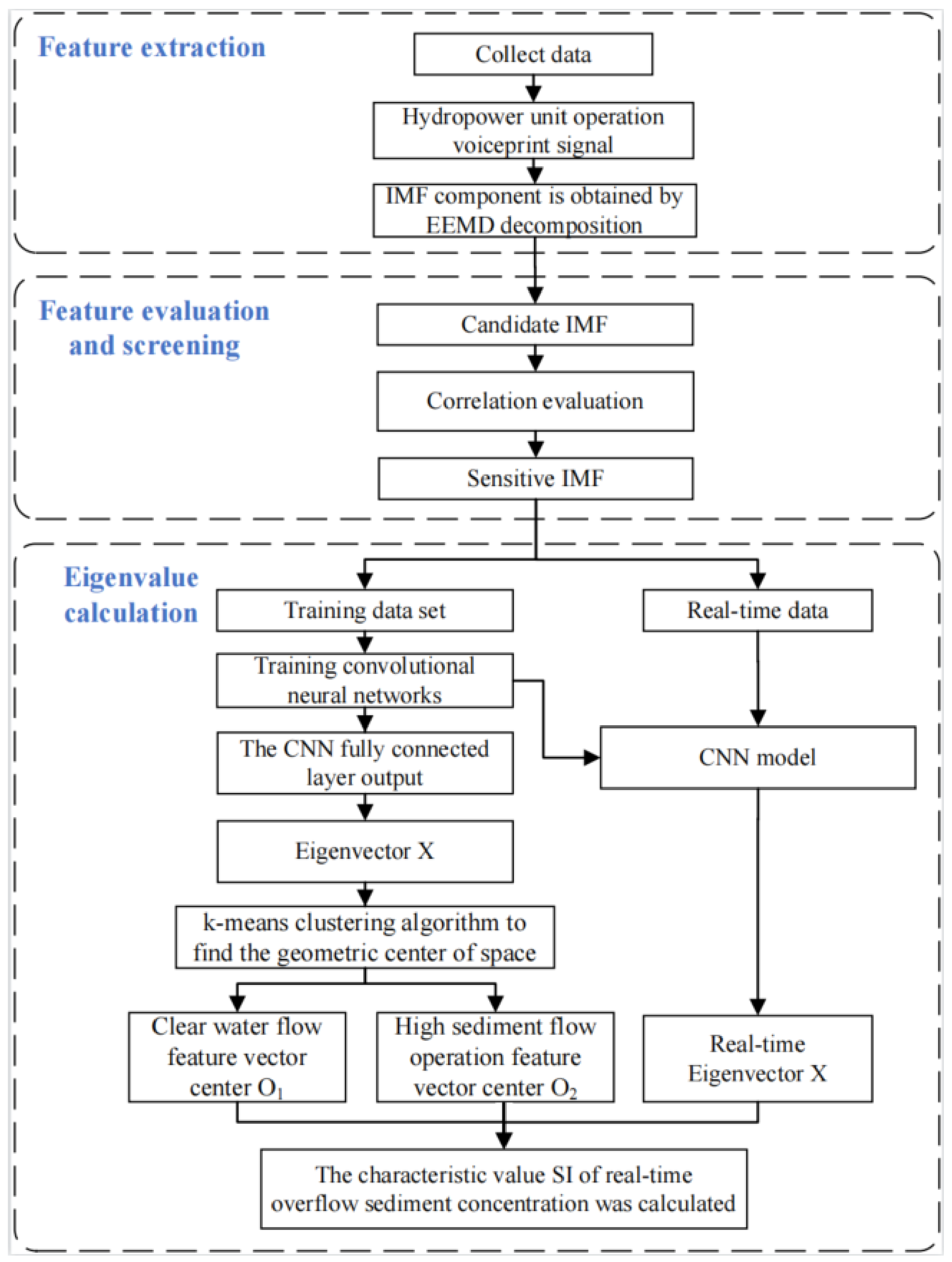
3. Feature Extraction of Flow Sediment Content of Hydropower Unit Based on Voiceprint Signal

In this study, a feature extraction method for the flow sediment content of hydropower units based on a voiceprint signal is presented. In this method, the voiceprint signal data of hydropower units with clean water flow and high sediment flow were first collected, and the collected voiceprint signals were decomposed by the Ensemble Empirical Mode Decomposition (EEMD) to obtain several intrinsic mode functions (IMF). This step corresponds to the feature extraction section in Figure 2. The obtained IMFs were analyzed by correlation, and IMF components that showed obvious characteristics of the unit’s operating status were retained. This step corresponds to the feature evaluation and screening shown in Figure 2. Input it into the convolutional neural network, and obtain the trained convolutional neural network model. After that, the multi-dimensional vector output from the fully connected layer of the convolutional neural network was extracted to form the feature vector sets of the hydropower unit with clean water flow and high sediment flow in different operating states, and the geometric centers of the corresponding feature vector sets under different operating states were obtained by using the k-means clustering algorithm. The center of the running feature vector of clean water is $O_1\left(x1,x2,\dots ,xn\right)$, and the center of the running feature vector of the flow with high sediment flow was $O_2\left(y1,y2,\dots ,yn\right)$. The distance $D$ of $O_1$ and $O_2$ is obtained by using the Euclidean distance method, as shown in Equation (10).

$$D=\sqrt{{\displaystyle \sum }_{i=1}^n{\left(x_i-y_i\right)}^2}$$

(10)

After that, the real-time operation voiceprint data of the hydropower units were collected, decomposed by EEMD, screened by correlation, and input into the trained convolutional neural network model to extract the multi-dimensional feature vector $X$ of the fully connected layer (as shown in Figure 1). The distance $D_1$ from vector $X$ to the center of the normal state feature vector $O_1$ was obtained by using the Euclidian distance method, and Formula (11) was adopted. The unit sediment concentration characteristic index is calculated, named $SI$:

$$SI=1-\frac{D_1}{D}$$

(11)

This corresponds to the eigenvalue calculation section in Figure 2.

A few points to discuss:

(1) According to the definition of Equation (10), $D$ is the calculated value under a fixed sediment particle size and sediment concentration, and this sediment condition becomes the standard sediment test condition. The corresponding vector distance $D$ is also called the standard distance. The size of the $D$ value only reflects the vector distance between the sand-bearing flow and the clear water, and the larger the $D$ value is, the larger the sand content in the water is.

(2) The physical meaning of $D_1$ in Formula (11) is exactly the same as that of $D$, and the index $SI$ reflects the degree of deviation of the sand-bearing flow from the standard sediment test conditions. When the sample flow sediment content is small or the flow is water, the calculated vector $X$ is close to the center of the normal operation eigenvector $O_1$, the calculated value of $D_1$ is small or close to 0, and the $SI$ value is close to 1. The higher the sediment content, the larger the vector distance $D_1$, the larger the $D_1/D$ value, and the smaller the SI value. When the excess sediment content of real-time samples exceeds all existing samples, the distance between vector X and the center of the normal feature vector $O_1$ is very far, $D_1$ is greater than $D$, and the value of $D_1/D$ is greater than 1, and the calculated $SI$ value is negative.

(3) This definition reduces the strict definition of standard sediment test conditions. In practical applications, it is only necessary to formulate a standard sediment flow for test calculation $D$ according to river sediment conditions. The $SI$ obtained by real-time test analysis can be approximately converted to the corresponding sediment content according to this relative value.

In summary, the closer the $SI$ value is to 1, the better the flow quality is. The closer the $SI$ value is to 0 or negative, the larger the flow sediment concentration is. Based on the $SI$ value, the characteristic value of flow sediment concentration of hydropower units can be observed in real time, and the change in flow sediment concentration of hydropower units can be mastered. The extraction process of the flow sediment content feature of the hydropower unit based on a voiceprint signal is shown in Figure 2.

4. Test Results and Analysis

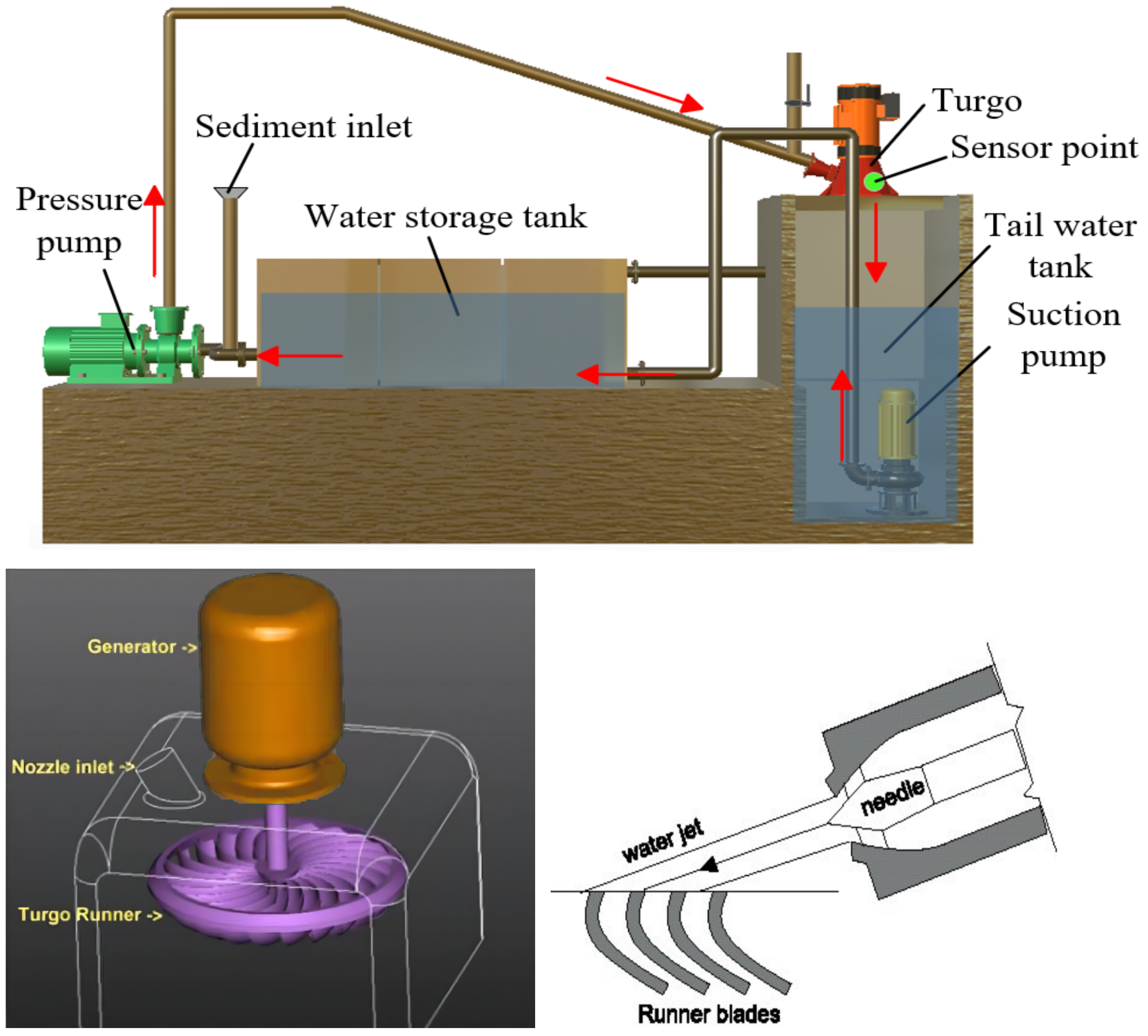
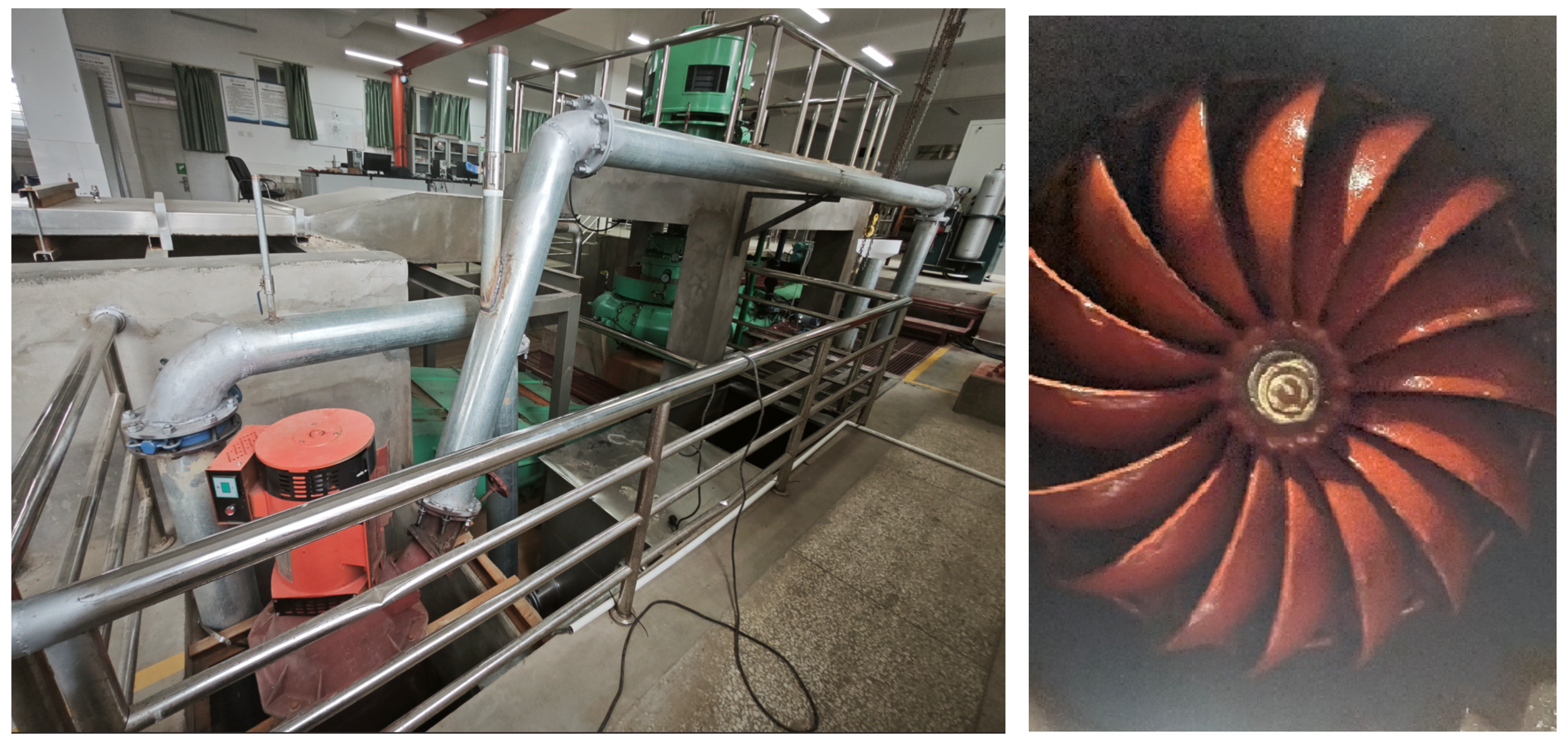
4.1. Test Bench

In order to verify the effect of flow sediment concentration feature extraction for hydropower units, a test rig was designed and built, as shown in Figure 3. The red arrow shows the direction of the flow. The test bed consists of four parts: a water tank, a water supply system, a water turbine generator set, and a return water system. The water supply system includes pressure pumps, pipes, and valves, and the return water system is composed of pumping pumps, pipes, and valves. The test bench entity is shown in Figure 4. The unit on the test bench is a Turgo turbine, and the parameters are shown in

Table 1. Turgo main geometrical and nominal operation data.

Runner Diameter/cm	Number of Runner Blades	Nozzle Diameter/mm	Distance from Nozzle to Blade/cm	Pipe Diamter/cm	Flow Rate/m3·h−1	Pressure Pump Head/m	Rated Speed /rpm
25	16	28	12	15	120	15	1500

. The test stand is used to measure the grinding and voiceprint signals of the hydropower unit. Water is injected into the water tank and tailwater tank before the test stand is run, and then the pressure pump and the pump are started at the same time. The pressure pump will press the water in the water tank and flow to the hydrogenerator along the pipeline, impact runner blades, and the water flowing through the hydrogenerator enters the tailwater tank, and then the water is pumped back to the water tank through the pump to complete the cycle.

The signal acquisition device used a voiceprint sensor, model CRY2301. The sensor is an industrial-grade small voiceprint real-time spectrum analyzer that has an advanced DSP processor, microphone, preamplifier, and data acquisition card in one and ensures accurate and efficient data processing under the premise of a tight structure arrangement. At the same time, the CRY2301 has built-in frequency time meter weight filtering and can perform acoustic analysis functions such as voiceprint statistical analysis, octave analysis, and FFT analysis. Parameters of the voiceprint sensor are shown in

Table 2. Noise sensor CRY2301 parameters.

Parameter Name	Specification
Sampling rate	48 kHz
Measurement frequency range	10~20,000 Hz
Standard measuring range	25~130 dBA
Measurement dynamic range	$\ge$110 dBA
Communication interface	USB Audio + USB SID

.

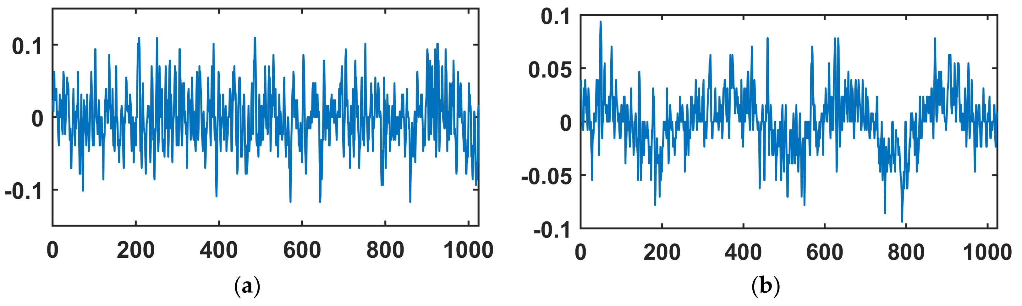
4.2. Data Collection

The sampling frequency of the data acquisition system was 10,240 Hz.

Test process:

(1) The voiceprint signal of the collection unit when the clean water was running;

(2) During the operation of the unit, quantitative sediment is poured into the turbine runner at a constant speed within 2 s through the sediment inlet pipe, so that the sediment enters the turbine runner according to certain rules;

(3) There was a filter in the tail tank, which can prevent sediment from entering the tank and affecting the subsequent test;

(4) Collect continuous voiceprint signal data on sediment passing through the turbine runner;

(5) The sampled data are divided into 25 sample data in a time slice of 0.1 s.

Sample number 15 in the two groups of clean water flow and high sediment flow is shown in Figure 5. Among the samples with high sand flow, sample number 15 is the sample with the lowest SI value in subsequent calculations, while the voiceprint data collected in the clean water flow are similar in waveform. Sample number 15 is also taken here for comparison.

(6) In this experiment, the tap water in the water tank of the experimental platform is clean water. The sediment concentration of the simulated high sediment content flow is 1.492 × 10⁵ mg/L. We pour 10 kg of sediment with a particle size of 2 mm into the pipeline within 2 s, and the flow rate of the pump is 120 m³/h. A total of 67 L of water and 10 kg of sediment are provided to the unit within 2 s, and the sediment concentration is 1.492 × 10⁵ mg/L. However, because the sediment is not immediately fully integrated with 67 L of water after pouring, the concentration has a gradual increasing process, and some sediment has entered the unit in this process, so the sediment concentration in the actual pipeline should be slightly less than the calculated concentration of 1.492 × 10⁵ mg/L.

In Figure 5, the horizontal coordinate represents the data point, and the vertical coordinate represents the relative sound pressure level; the unit of measure is Pa.

The collected voiceprint signals were first decomposed by EEMD, and the results were obtained as shown in Figure 6. The IMF number obtained by EEMD decomposition for 50 samples in this group is different in some cases, but the IMF of order 9 has reached the termination condition of EEMD decomposition, and the final 9 IMF and a residual res signal are shown in Figure 6.

In Figure 6, the horizontal coordinate represents the data point, and the vertical coordinate represents the relative sound pressure level; the unit of measure is Pa.

The correlation coefficient between each IMF and the original signal is calculated. The calculated results of the correlation coefficient between each IMF order under the two states are shown in Figure 7. It can be seen that the correlation between the IMF orders 8, 9, and 10 and the original signal is very low, while the correlation between the IMF orders 1, 2, 3, and 4 is high, which can better reflect the characteristics and changing trend of the original signal. The correlation coefficient of IMF in the 6th order fluctuates greatly, and some samples have a high correlation coefficient. The IMF of the 5th to 6th order is also taken as the characteristic data of the samples, and the IMF of the 1st to 6th order is finally selected to form the sample collection together.

The obtained samples were divided into two groups of 50 samples, with the ratio of the training set to the test set being 8:2. The convolutional neural network was the input for the training. Finally, the model with the highest accuracy was selected to extract the multi-dimensional feature vector of the samples. The parameters of the convolutional neural network are shown in

Table 3. Convolutional neural network parameter configuration.

Structure	Parameter Configuration	Data Dimension	Structure	Parameter Configuration	Data Dimension
Input layer	—	1 × 6 × 1024	Activation layer 2	ReLu	16 × 7 × 516
Convolution layer 1	In channel = 1	8 × 8 × 1026	Pooling layer 2	MaxPool2d	16 × 3 × 258
	Out channel = 8		Convolution layer 3	In channel = 16	32 × 6 × 264
	Kernel size = 3			Out channel = 32
	Stride = 1			Kernel size = 3
	Padding = 2			Stride = 1
Activation layer 1	ReLu	8 × 8 × 1026		Padding = 2
Pooling layer 1	MaxPool2d	8 × 4 × 513	Activation layer 3	ReLu	32 × 6 × 264
Convolution layer 2	In channel = 8	16 × 7 × 516	Pooling layer 3	MaxPool2d	32 × 3 × 132
	Out channel = 16		Fully connected layer 1	32 × 3 × 132, 6	6
	Kernel size = 2		Fully connected layer 2	6	2
	Stride = 1		classifier	Softmax	—
	Padding = 2		—	—	—

.

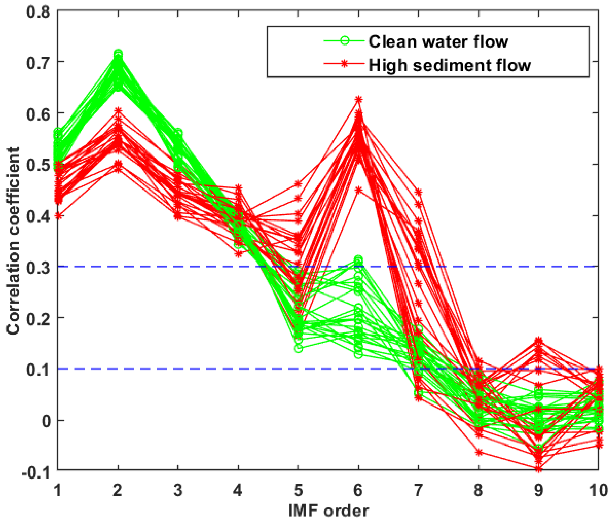
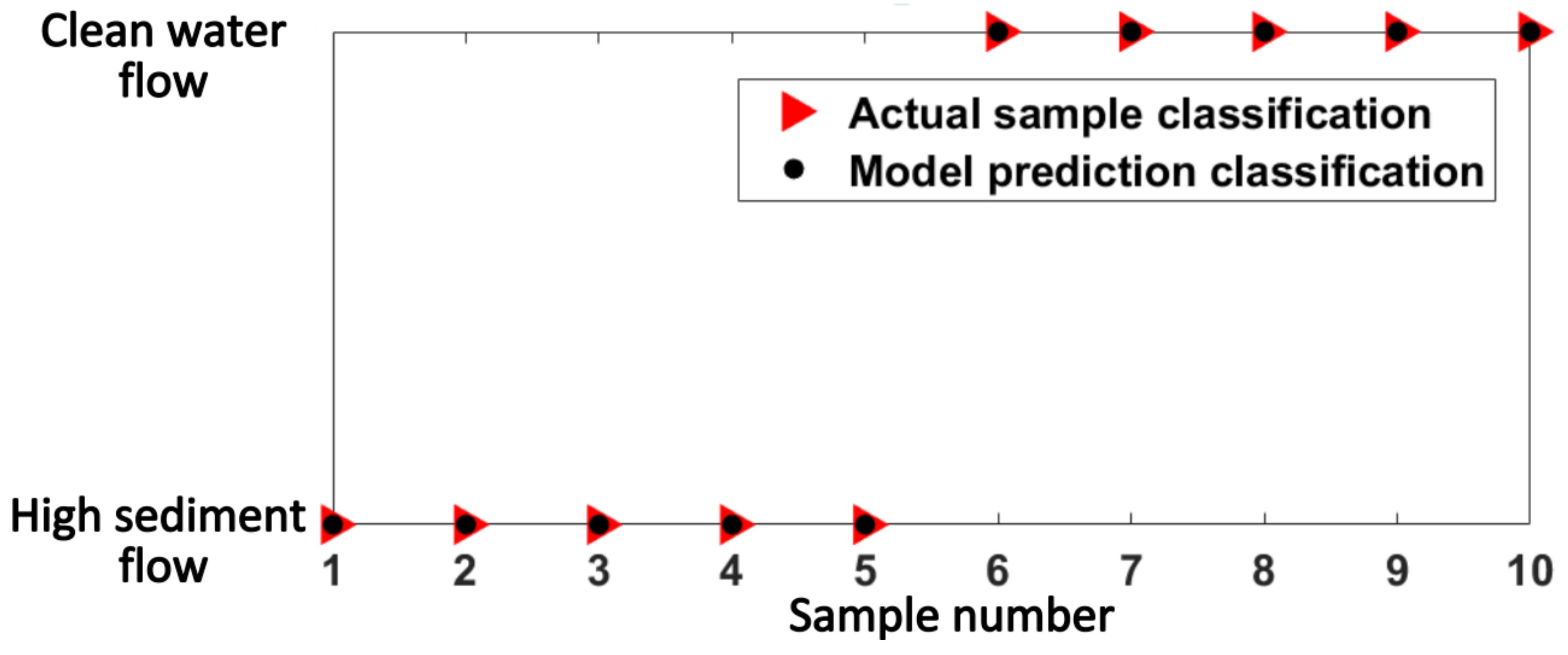
4.3. Result Analysis

The convolutional neural network model with a recognition rate of 100% is finally obtained after repeated training several times; each iteration is 30 times, and its recognition effect is shown in Figure 8.

A convolutional neural network model with 100% accuracy in recognizing two states was trained, its parameters were saved, and the 6-dimensional feature vector output from the full connection layer was extracted to form a feature vector set. Some feature vectors are shown in

Table 4. Two kinds of feature vector sets.

	Sample Number	Dimension 1	Dimension 2	Dimension 3	Dimension 4	Dimension 5	Dimension 6
Clean water flow	15	−9.0093	6.4762	8.0257	−7.9252	−6.6284	5.4979
	16	−9.8645	7.3514	8.93	−8.8102	−7.505	4.675
	17	−10.0583	7.6418	9.1117	−9.0261	−7.7321	4.2243
	18	−9.0093	6.4762	8.0257	−7.9252	−6.6284	5.4979
	19	−10.2709	7.7413	9.3238	−9.2237	−7.8838	4.3558
High sediment flow	35	16.4597	−18.2944	−17.3323	17.2836	18.2946	28.5648
	36	26.8568	−27.8913	−27.5007	27.6373	27.875	35.9686
	37	20.1545	−21.8032	−20.9024	21.0477	21.6961	30.4255
	38	23.1942	−24.5938	−23.9545	24.0666	24.5519	33.6247
	39	24.7757	−25.7658	−25.3686	25.4017	25.6819	33.5591

.

The k-means clustering algorithm was adopted to obtain the coordinates of the health centers in the two states as follows:

Clean water flow feature vector center $O_1$:

−9.787184615, 7.287619231, 8.834742308, 8.730161538, 7.422069231, 4.582080769

High sediment flow feature vector center $O_2$:

22.06903333, −23.51045833, −22.79761667, 22.88625417, 23.47661667, 32.43155

t-SNE (t-distributed neighbor embedding) is a machine learning algorithm used for dimensionality reduction. It is a nonlinear dimensionality reduction algorithm that is suitable for high-dimensional data to be reduced to 2 or 3 dimensions for visualization. For points with greater similarity, the distance in the low-dimensional space of the T-distribution will be smaller. For points with low similarity, the distance of the t distribution in low-dimensional space is far. It should be noted that the t-SNE middle distance is meaningless; it is a probability distribution problem, and the horizontal and vertical coordinates have no practical significance.

t-SNE dimensionality reduction is used to show the position of cluster centers in the feature vector set under the two-dimensional plane, as shown in Figure 9.

As shown in Figure 9, the 6-dimensional feature vectors extracted in the two states of the convolutional neural network are clearly separated in space, which confirms the accuracy of the convolutional neural network model training. The vector centers of the two states are also in the geometric centers of their eigenvector sets, which verifies the accuracy of the k-means algorithm in obtaining the vector center.

The Euclidean distance D between $O_1$ and $O_2$ was calculated, and the sediment characteristic value $SI$ of all samples was calculated, as shown in Figure 10.

Analysis of the results:

(1) The calculated $SI$ values of clean water flow samples all fluctuate near the value 1, and the analysis reasons are as follows: Due to the lack of sediment interference, the voiceprint data of clean water flow samples will not change greatly, and the waveforms among all samples are similar. The feature vector $X$ extracted in the convolutional neural network is closer to $O_1$, the center of the feature vector of clean water operation, and the value of $D_1$ is small. As can be seen from Formula (11), the value of $D_1/D$ is close to 0, and the final calculated $SI$ value is close to 1. The $SI$ value of 25 samples fluctuated slightly, which was analyzed as being caused by various hydraulic and mechanical factors and acquisition errors during the operation of the unit.

(2) Under the operation of sand-bearing flow, the $SI$ value presents an obvious trend of first decreasing and then increasing, and the reasons are analyzed as follows: As a large amount of sediment is poured into the pipeline at one time, the content of sediment in the pipeline increases. First, part of the sediment is preferentially pumped into the water turbine unit, causing changes in the voiceprint signal of the unit. At this time, the feature vector $X$ of the collected sample starts to move away from the water in space, the feature vector center $O_1$, and the value $D_1$ increases, which can be seen from Formula (11). The $D_1/D$ value increases accordingly, resulting in a decrease in the calculated $SI$ value. Corresponding to the first two samples in the sand-containing flow state in Figure 10, the SI value drops to about 0.2. After that, the sediment poured into the pipeline is continuously pumped into the hydropower unit. The sediment content in the flow continues to increase, and the calculated SI value continues to decrease. This process corresponds to samples 3–14 in Figure 11. At sample 15, the sediment content in the flow reaches the peak value, and the calculated $SI$ value is 0.06. After the sediment content reached the peak, the pressure pump continued to pump the clean water in the tank, but no more sediment was poured into the water, resulting in a continuous decrease in the sediment content in the flow, and the SI value gradually increased, corresponding to samples 16–25 in Figure 10. Eventually, all the sediment is pumped into the hydropower unit and left in the tailwater tank, and the flow into the hydropower unit returns to clean water.

In order to verify the effectiveness of the proposed method for extracting sediment features from flow, the experiment was conducted by using different modes of sediment pouring with the same particle size. Other test bench parameters are the same as previously mentioned. The continuous voiceprint data during the collection process were selected. At the same time, the first 5 sample lengths with changes in each method were selected as the starting point of the data, and the $SI$ value in the process was calculated using the proposed method. The sediment data for different test methods are shown in

Table 5. Sediment data for different test methods.

	Dumped Sediment Mass	Pour Time	Theoretical Maximum Sediment Content
Method 1	10 kg	2 s	1.492 × 105 mg/L
Method 2	10 kg	3 s	1 × 105 mg/L
Method 3	5 + 5 kg	1 s + 1 s (interval) + 1 s	1.492 × 105 mg/L

.

Method 1: A large amount of sediment is poured at one time (same as this method).

Method 2: Sediment is poured slowly and continuously for 3 s.

Method 3: Much sediment is poured at 2 intervals of 1 s, and the time of each pour is controlled within 1 s.

$SI$ values were calculated using the method presented in this paper, as shown in Figure 11.

In summary, it is proven that the method in this study can complete the extraction of the flow sediment content characteristics of the unit, which is of great significance for improving the maintenance level of the unit state, curbing the fault spread, and reducing the fault loss.

5. Conclusions

Hydraulic turbine operation is often accompanied by sediment wear, and the flow sediment content is an important parameter characterizing hydraulic machinery abrasion. In this study, a method of flow sediment content feature extraction for hydropower units based on a voiceprint signal is proposed, which can extract the characteristic value of flow sediment content of hydropower units in real time and master the change in flow sediment content of hydropower units. The experimental results show that this method can complete the extraction of the flow sediment content characteristics of the unit, which is of great significance for improving the maintenance level of the unit state, curbing the fault spread, and reducing the fault loss.

Outlook: There are very few reference cases to carry out feature extraction research on the flow sediment content of hydropower units based on voiceprint signals. We can only verify the feasibility of the proposed method and the feasibility of the application of voiceprint signal detection technology in feature extraction of hydropower units with sediment content based on existing experimental conditions, so as to establish a foundation for further research. In the future, we will continue to further establish the exact correspondence between the characteristic value $SI$ and the concentration and make further contributions to the development of the hydropower unit fault diagnosis field.

References

1. Li, Y.; Zhu, Y.; Xiao, Y. Numerical analysis of bucket hydro-abrasive erosion in a Impulse turbines on sediment season. J. Hydroelectr. Eng. 2024, 2, 1–8. [Google Scholar]
2. Padhy, M.K.; Saini, R.P. A review on silt erosion in hydro turbines. Renew. Sustain. Energy Rev. 2008, 12, 1974–1987. [Google Scholar] [CrossRef]
3. Khurana, S.; Varun Kumar, A. Effect of silt particles on erosion of Turgo impulse turbine blades. Int. J. Ambient Energy 2014, 35, 155–162. [Google Scholar] [CrossRef]
4. Rai, A.K.; Kumar, A. Continuous measurement of suspended sediment concentration: Technological advancement and future outlook. Measurement 2015, 76, 209–227. [Google Scholar] [CrossRef]
5. Rai, A.K.; Kumar, A.; Staubli, T. Effect of concentration and size of sediments on hydro-abrasive erosion of Pelton turbine. Renew. Energy 2020, 145, 893–902. [Google Scholar] [CrossRef]
6. Rai, A.K.; Kumar, A. Sediment monitoring for hydro-abrasive erosion: A field study from Himalayas, India. International. J. Fluid Mach. Syst. 2017, 10, 146–153. [Google Scholar] [CrossRef]
7. Zhou, X. Design of equipment fault diagnosis system based on audio analysis technology. J. Phys. Conf. Ser. 2023, 2433, 012033. [Google Scholar] [CrossRef]
8. Huang, X.; Su, Z.; Sgu, S.; Rao, Z.; Hua, H. Vibroacoustic radiation of pump-.Jet hull coupling system under distributed pulsating pressure excitation. J. Vib. Shock 2021, 40, 1–9. [Google Scholar]
9. Tang, Y.J.; Zhou, X.J.; Zhang, F. Application of noise analysis in fault diagnosis of hydropower units. J. China Rural. Water Hydropower 2017, 8, 206–208. [Google Scholar]
10. Ni, J.; Hu, C.; Zhao, M. A ship radiation noise identification method based on VMD and improved CNN. J. Vib. Shock 2023, 42, 74–82. [Google Scholar]
11. Zhou, S.; Hong, J.; Huang, C.J. Research on On-line Monitoring of tool wear State based on Acoustic emission Signal analysis. J. Tool Technol. 2022, 56, 51–55. [Google Scholar]
12. Weng, Z.; Ll, N.; Yuan, J.; Liu, H.; Sun, X.; Hao, M.; Si, J. Friction state recognition of liquid film seal based on acoustic emission time-frequencyanalysis and convolution neural network. J. Lubr. Eng. 2023, 48, 136–141. [Google Scholar]
13. Huang, N.E.; Shen, Z.; Long, S.R.; Wu, M.C.; Shih, H.H.; Zheng, Q.; Yen, N.-C.; Tung, C.C.; Liu, H.H. The empirical mode decomposition and the Hilbert spectrum for nonlinear and nonstationary time series analysis. Proc. R. Soc. Lond. Ser. A 1998, 454, 903–995. [Google Scholar] [CrossRef]
14. Wu, Z.H.; Huang, N.E. Ensemble Empirical Mode Decomposition: A noise-assisted DATA analysis method. J. Adv. Adapt. Data Anal. 2009, 1, 1–41. [Google Scholar] [CrossRef]
15. He, K.D.; Jia, C.H.E.N.; Yan, J.I.N.; Jiang, W.J.; Xiao, Z.H. Application of EEMD multi-scale entropy and ELM in feature extraction of vibration signal of hydropowerunit. J. China Rural. Water Hydropower 2021, 176, 187. (In Chinese) [Google Scholar]
16. Yang, S.S.; Kim, Y.G.; Choi, H. Vehicle identification using discrete spectrums in wireless sensor networks. J. Netw. 2008, 3, 51–63. [Google Scholar] [CrossRef]
17. Sun, Z.; Machlev, R.; Wang, Q.; Belikov, J.; Levron, Y.; Baimel, D. A public data-set for synchronous motor electrical faults diagnosis with CNN and LSTM reference classifiers. J. Energy AI 2023, 14, 100274. [Google Scholar] [CrossRef]
18. Jasim, H.A.; Ahmed, S.R.; Ibrahim, A.A.; Duru, A.D. Classify bird species audio by augment convolutional neural network. In Proceedings of the 2022 International Congress on Human-Computer Interaction, Optimization and Robotic Applications (HORA), Ankara, Turkey, 9–11 June 2022; pp. 1–6. [Google Scholar]
19. Chen, G.; Zhang, X.; Zhang, J.; Li, F.; Duan, S. A novel brain-computer interface based on audio-assisted visual evoked EEG and spatial-temporal attention CNN. J. Front. Neurorobotics 2022, 16, 995552. [Google Scholar] [CrossRef]
20. Liu, X.; Liu, J.; Yu, L. Signal processing of photoelectric weapon RF test based on EEMD. J. Artill. Launch Control 2023, 44, 19–23. [Google Scholar]
21. Xiao, J.; Jin, J.; Li, C.; Xu, Z.; Luo, S. Fault diagnosis of wind turbine gearboxes based on deep learning. J. Sol. Energy 2023, 44, 302–309. [Google Scholar]
22. Ksibi, A.; Hakami, N.A.; Alturki, N.; Asiri, M.M.; Zakariah, M.; Ayadi, M. Voice pathology detection using a two-level classifier based on combined CNN–RNN architecture. Sustainability 2023, 15, 3204. [Google Scholar] [CrossRef]
23. Yan, R.; Lin, C.; Song, W.; Gao, S.; Zhong, L.; Zhang, W. Research on circuit breaker fault diagnosis based on EEMD and convolutional neural network. J. High Volt. Appar. 2022, 58, 213–220. [Google Scholar]
24. Wang, H.; Zhu, J.; He, Z. Multivariable water level prediction model based on convolution radial basis network. J. Hydroelectr. Eng. 2023, 42, 70–81. [Google Scholar]
25. Chen, Y.; Yang, L.; Li, S. Traffic congestion prediction algorithm based on CS-BiLSTM framework. J. Sci. Technol. Eng. 2022, 22, 12917–12926. [Google Scholar]
Figure 1. Convolutional neural network structure diagram.
Energies 17 01041 g001
Figure 2. Feature extraction process of flow sediment content of a hydropower unit based on a voiceprint signal.
Energies 17 01041 g002
Figure 3. Schematic diagram of the three-dimensional model of the test bench.
Energies 17 01041 g003
Figure 4. Test bench.
Energies 17 01041 g004
Figure 5. Voiceprint signal data. (a) Clean water flow data; (b) high sediment flow data.
Energies 17 01041 g005
Figure 6. EEMD results. (a) Clean water flow results; (b) high sediment flow results.
Energies 17 01041 g006
Figure 7. IMF correlation coefficients for each order.
Energies 17 01041 g007
Figure 8. Recognition effect of a convolutional neural network.
Energies 17 01041 g008
Figure 9. Location of cluster centers.
Energies 17 01041 g009
Figure 10. S I index values of all samples.
Energies 17 01041 g010
Figure 11. S I values of three sediment dumping methods.
Energies 17 01041 g011