Abstract
When the overhead line passes through the forest area, the conductor may contact the line to induce the tree-contact single-phase-to-ground fault (TSF), and the persistence of TSF may induce wildfires, bringing serious consequences. However, the amount of TSF electrical features is weak, and traditional protection devices cannot operate effectively, so it is urgent to obtain typical characteristics of TSF. In this study, the simulation experiment is carried out for the tree-contact single-phase-to-ground fault. Firstly, the relativity between fault and characteristics like zero-sequence voltage, zero-sequence current, and differential current are analyzed theoretically. Then, the simulation experiment platform of TSF is built, and the time-varying fault characteristics are acquired. The experimental results show that the average value of the zero-sequence voltage, the amplitude of the power-frequency component of the zero-sequence current, and the amplitude of the power-frequency component of the first and end differential current can accurately reflect the fault current development trend of the single-phase contact tree fault of the conductor, and can be used as the typical characteristic quantity of TSF. The results of this study are helpful for further understanding the fault characteristics of TSF and provide theoretical support for the identification and protection design of TSF.
1. Introduction
As the scale of the power grid gradually expands, an increasing number of distribution lines cross densely vegetated forested areas [1]. And when the 10 kV distribution network overhead line traverses through mountainous forest regions, it can be influenced by external factors, such as lightning strikes or strong winds. This can lead to contact between the overhead line and the higher branches of trees, resulting in a discharge, which creates a single-phase grounding fault [2], which is defined as a tree-contact single-phase-to-ground fault (TSF). The prolonged existence of the TSF can potentially trigger wildfires, posing a serious threat to the safety of residents’ lives and properties [3]. For example, in November 2018, the state of California in the United States experienced a wildfire caused by a transmission line failure, resulting in economic losses of billions of dollars [4,5]. In March 2020, in Liangshan Prefecture, Sichuan Province, China, a massive wildfire was triggered by electrical faults that caused insulation materials to ignite and fall, igniting surface litter and resulting in significant damage [6,7]. It can be seen that TSF’s detection and recognition have great significance for the safety of residents’ lives and property and the safe and stable operation of the power system.
However, the detection and effective recognition of TSF still remains a challenging task that requires significant effort. Upon investigation, it is believed that the main reasons can be summarized as follows. Firstly, the transition resistance of the TSF is huge, reaching hundreds of kiloohms [4,8], which results in weak electrical characteristics. For example, the fault current is only a few hundred milliamperes. This results in fault currents failing to reach the activation setpoint for protection devices during the TSF, rendering traditional overcurrent protection devices inoperative [9]. Secondly, limited by the operability and safety of TSF experiments and the differences in tree species and sizes, it is difficult to conduct on-site experiments to cover all scenarios, resulting in a small amount of measured data [9,10]. Finally, the TSF involves botanical theories such as tree growth conditions and internal structure. And the development and evolution process, characteristic parameter changes, rules, and mechanisms of TSF have not been fully understood. Therefore, it is urgent to obtain typical characteristic parameters of the TSF in order to lay a foundation for further research on fault detection and recognition algorithms.
Many researchers at home and abroad have conducted relevant studies around analyzing and extracting TSF characteristic parameters. Butler et al. from Texas A&M University simulated single-phase tree-contact ground faults on a 12.5 kV three-phase transmission line, obtaining information such as images, sounds, voltage gradients, and leakage current during the fault [11]. Jeffer et al. found through analysis that the fault current increases with the increasing degree of carbonization [12]. Gomes et al. used a sparse coding technique to extract high-frequency characteristics from the TSF, which can be used for fault detection [13]. SEDIGHI et al. used two artificial intelligence algorithms, a genetic algorithm and an artificial neural network, as the foundation. They combined the high-frequency transient components of fault currents after wavelet transform and used them as inputs for the neural network method to detect high-resistance ground faults [14].
However, in practical applications, the operability of the above-mentioned methods is still relatively low. Firstly, most fault detection algorithms have poor recognition performance for high-resistance scenarios. According to existing research results, the initial transition resistance of the TSF can reach the Megaohm level [8]. By the time it develops into resistance easily recognized as a few hundred ohms, the trees have already caught fire. At this point, completing the recognition has limited significance. Secondly, the distribution of the distribution network system is extensive, making it impractical to collect images, sounds, and other information in every area. As a result, the main basis for the final judgment still relies on characteristic quantities such as current and voltage [15]. Moreover, if only one parameter is used to identify TSFs, it is highly susceptible to interference and can lead to misjudgments. For example, using only zero-sequence voltage to identify TSFs can lead to misjudgments. This is because an unbalanced operation of the system can generate zero-sequence electromotive forces, which can interfere with the fault identification process. Lastly, the TSF can have multiple different fault-development processes depending on parameters such as tree length, thickness, and species. However, the aforementioned research does not discuss the recognition performance under diverse scenarios. It can be seen that there are still significant technical gaps in the identification of TSFs. How to extract fault features using easily detectable data such as current and voltage is an important problem that urgently needs to be addressed.
To address the above issues, this study builds a simulation experimental platform for 10 kV distribution network lines, using three common trees such as natural growth Cinnamomum camphora, Bauhinia blakeana, and pine as experimental objects, and analyzes the tree line discharge fault characteristics under different parameters. The experiment simultaneously measures various parameters such as phase voltage, zero-sequence voltage, zero-sequence current, fault phase incoming and outgoing line current, and leakage current. Taking the leakage current at the fault point as the basis for the fault-development trend, the data are processed to extract fault feature quantities, and the effect of the extracted fault feature quantities is studied under different tree species, different lengths, and different thicknesses in various fault scenarios.
2. Main Characteristic Quantities of the TSF
2.1. Main Characteristics of the TSF
Accurately extracting fault characteristics is the foundation for fault identification. As a special type of single-phase high-resistance ground fault, the TSF has the following three characteristics compared to other types of faults:
- (1)
- Referring to the equivalent resistance from the tree-line contacting point to the ground, occurring during the TSF, the transition resistance is very high, which is mainly due to the significant contact resistance between the conductor and the tree branches. The contact resistance is in the range of 105 to 106 Ω [4,8], which results in very small fault currents, causing the characteristic quantities used for protection in the line to be unable to exceed the threshold. Therefore, traditional protection devices have difficulty operating in such cases;
- (2)
- During the development of the TSF, the current passing through the tree causes the temperature of the tree to gradually increase. Before the occurrence of visible fire and complete carbonization of the tree, the transition resistance of the TSF shows a decreasing trend [8], which leads to an increasing fault current;
- (3)
- In the case of the TSF, there is a fault arc between the line and the trees. The action of AC voltage causes the arc to continuously extinguish and reignite, resulting in a noticeable “zero crossing” phenomenon of the fault current [16]. This will lead to the generation of high-frequency signals and harmonic signals.
It can be seen that the fault current in the TSF is small, making it difficult to directly identify faults through traditional protection methods based on the zero-sequence current and voltage signals crossing preset values. The “zero crossing” phenomenon observed in the TSF is mainly caused by the presence of fault arcs. The harmonics and high-frequency signals generated during this process are not unique characteristics of TSFs. Additionally, considering the actual operating conditions of the system, these harmonics and high-frequency signals can also be present during normal operation. Furthermore, due to the presence of noise interference, it is difficult to directly determine TSFs based on the aforementioned harmonics and high-frequency signals. Therefore, the increasing trend of the fault current during the development of the TSF can be considered a unique characteristic of the TSF and can be used as a basis for its identification and determination. However, in practical systems, it is not always possible to directly measure the fault current. Therefore, it is necessary to examine the electrical signals that change along with the fault current and can be measured. These signals can be used to reflect the changing trend of the fault current and, based on these signals, complete the fault identification. As the line often uses parameters such as zero-sequence voltage and zero-sequence current to determine faults, and the differential current at the faulted phase terminals is close to the fault current in the measurable signals, this study will focus on the commonly used and measurable electrical signals. Firstly, it will analyze the changes in fault current during the development of the TSF. Then, based on the fault current, it will analyze the variations in the zero-sequence voltage, zero-sequence current, and differential current at the faulted phase terminals during the TSF process. During the operation of the power system, factors such as weather and operational conditions can lead to system imbalance, resulting in zero-sequence voltage and so on. These fluctuations are transient and considered normal within a certain range. The impact of tree line discharge failures is long-lasting; most notably, the fault current increases steadily over time.
2.2. Theoretical Calculation
Many 10 kV distribution systems adopt ungrounded systems. In long transmission lines, the reactance of the line is significantly greater than its resistance, and it exhibits inductive characteristics. Meanwhile, in the distribution network, the line resistance exceeds the line reactance, and the latter exhibits capacitive behavior. However, for 10 kV ungrounded systems, due to the fact that the system’s capacitive impedance greatly exceeds its resistive impedance, the system impedance is capacitive. Figure 1 shows the equivalent model of a 10 kV distribution network during a single-phase ground fault. C0 represents the capacitance between the distribution network and the ground, and Rf represents the transitional resistance of the ground fault. Using the superposition principle, the circuit diagram can be simplified, as shown in Figure 1. In this diagram, Ueq represents the equivalent zero-sequence source voltage. When the three-phase capacitance of the distribution network is approximately balanced, Ueq = E, which represents the phase voltage of the system.
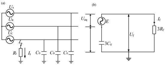
Figure 1.
Equivalent circuit of TSF. (a) Equivalent model of distribution network during single-phase ground fault, and (b) equivalent simplified circuit for single-phase ground fault.
With the development of the TSF, the transition resistance will gradually decrease with time [8]. According to Equation (1), the fault grounding current If will gradually increase. In this study, the fault current is used as a reference to evaluate the effectiveness of other fault characteristic parameters in reflecting the TSF.
The TSF zero-sequence network is shown in Figure 2. Among them, 3Uf0 is the fault zero-sequence voltage source, which can be considered as the system phase voltage E for high-resistance faults; 3I0 is the fault zero-sequence current; 3U0 is the bus zero-sequence voltage; 3Rf is the fault transition resistance; and 3C0 is the sum of the distribution network capacitance to ground.
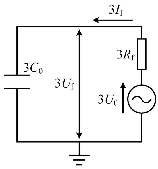
Figure 2.
Zero-sequence equivalent network of TSF.
From Figure 2, the zero-sequence voltage and current are shown, respectively. Among them, the ground capacitance C0 is a constant.
In this study, the differential current of the fault phase head and tail is defined as the difference between the current at the incoming end and the current at the outgoing end of the fault phase line. Assuming that the fault phase is phase C, the current flow model of the line fault phase in a neutral ungrounded system can be simplified, as shown in Figure 3.
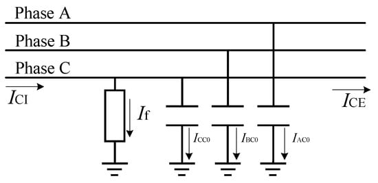
Figure 3.
Schematic diagram of the differential current of the head and the end of the fault phase.
According to Figure 3, the difference between the current ICI at the inlet terminal and the current ICE at the outlet terminal is the sum of the fault current If and the fault relative-to-ground capacitive current ICC0. Since the fault current is the sum of the system’s capacitive current to ground, the differential current ICD is equal to the sum of the B-phase capacitive current IBC0 and the A-phase capacitive current IAC0:
3. Design and Method of Experimental Platform
3.1. Experimental Platform and Layout
According to the actual operation of the 10 kV distribution network, a 10 kV distribution network experimental platform was built. The schematic diagram of the experimental platform is shown in Figure 4.
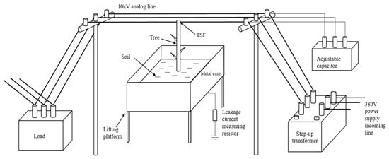
Figure 4.
Schematic diagram of the experimental platform.
The 10 kV voltage used by the platform is obtained from the 380 V power supply inlet through a step-up transformer. The transformer wiring is YNyn0 type, with the neutral point suspended. The three-phase distribution line uses steel-cored aluminum stranded wire with a model LGJ-120. To simulate a real fault situation, soil is installed in the lifting platform, branches are inserted into the soil, and the lifting platform is raised so that the branches rest on the C-phase of the distribution line, creating a tree-line discharge fault. The leakage current at the fault point flows through the sampling resistor and enters the ground. Measure the voltage waveform on the high-voltage side of the sampling resistor and connect the waveform to an oscilloscope. Then, the leakage current waveform can be obtained according to Ohm’s law. The capacitive current can be adjusted from 1 to 60 A, with a minimum differential of 1 A. Use an open delta connection to measure the zero-sequence voltage with a zero-sequence voltage transformer with a transformation ratio of 10:0.1 and an accuracy level of 0.5 s. Measure the zero-sequence current with a through-type zero-sequence current transformer with a transformation ratio of 150:5 and an accuracy level of 0.5 s. Measure the differential current with a differential current transformer with a transformation ratio of 40:5 and an accuracy level of 0.2 s. The experimental site photo is shown in Figure 5, and the measurement system in the experimental system is illustrated in Figure 6.
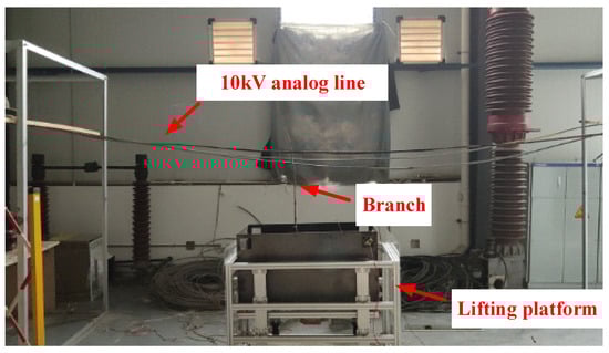
Figure 5.
Photo of experimental platform.
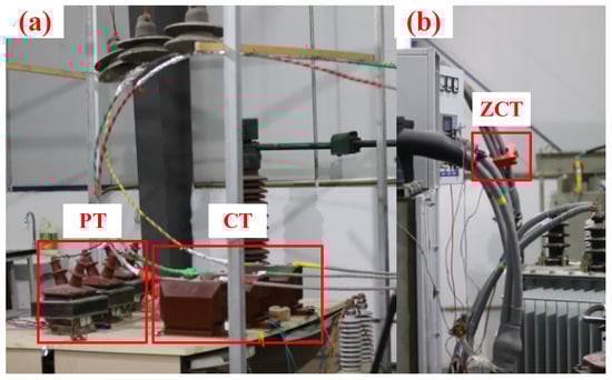
Figure 6.
The measurement system in the experimental system. (a) PT and CT, (b) zero-sequence CT.
3.2. Experimental Procedure
A total of seven branches were collected for this experiment, and experiments were conducted under the same conditions. The specific steps of the experiment are as follows:
- (a)
- Branches selection: In the experiment, branches of different lengths and thicknesses of Bauhinia, Cinnamomum camphora, and pine trees were selected as experimental objects. To avoid the branches and leaves overlapping to form short circuits and for ease of observation, the branches and leaves were cut off. Figure 7 shows an experimental sample, and the measured dimensions and parameters of some trees are shown in Table 1. The lengths mentioned in the table are the lengths of the branches from the point of failure to the point where the branch meets the ground, and the diameters are the diameters of the branches at the point of grounding;
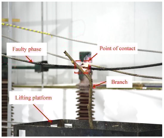 Figure 7. Schematic diagram of the experimental process.
 Table 1. Main parameters of experimental tree branches.
- (b)
- Experimental process: Before the experiment, one end of the branch is connected to the line, and the other end is buried in the soil of the lifting platform. After connecting the power supply, the experiment starts. The fault recording device is used to record the three-phase voltage, zero-sequence voltage, zero-sequence current, fault phase head, and tail current of the line. The acquisition time is 50 s. If the branch is burnt out, the experiment is stopped. After completing one set, the conditions remain unchanged, and the branch is replaced for the next set of experiments;
- (c)
- Data sorting: Sorting data, discarding data with large errors or measurement errors, and merging available data into datasets.
4. Analysis of Experimental Results
4.1. Basic Case Analysis
To analyze the development process of the TSF, branch No. 4 was used as the basic case, and the experimental results were analyzed. The experimental process of branch No. 4 is shown in Figure 7.
During the experiment, the fault current, fault phase voltage, and transition resistance of branch 4 exhibited changes over time, as illustrated in Figure 8. As evident from Figure 8a,b, the fault current gradually increased over time, whereas the fault phase voltage remained nearly constant. According to , the transition resistance gradually decreases over time, consistent with the trend of transition resistance shown in Figure 8c. Meanwhile, these results align with the analysis from the previous section.
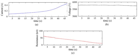
Figure 8.
The R-t plot of branch 4. (a) RMS value of current at the fault point, (b) RMS value of voltage at the fault point, and (c) transition resistance.
In the experiment, the instantaneous values of the fault current, zero-sequence voltage, zero-sequence current, and differential current were collected. However, considering that the instantaneous values change sinusoidally if the collected instantaneous values are directly used for judgment, the fluctuating data cannot reflect the development of the fault. Therefore, in order to more significantly observe the trend of numerical changes, calculating the RMS values of the above parameters can stabilize data fluctuations to a certain extent and reduce noise interference, thus more intuitively observing the trend of changes in the above parameters. For ease of comparison, the normal operation data measured under the same conditions in the experiment were processed identically and presented together in Figure 9.
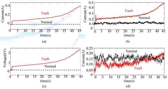
Figure 9.
RMS value of TSF characteristic quantity. (a) RMS value of fault current, (b) RMS value of differential current at the beginning and end, (c) RMS value of zero-sequence current, and (d) RMS value of zero-sequence voltage.
As shown in Figure 9a, when the TSF occurs, the fault current shows a gradual upward trend, while under normal operating conditions, the fault current is close to 0. As shown in Figure 9b,c, when the TSF occurs, the differential current and zero-sequence voltage waveforms are consistent with the fault current variation trend and significantly higher than the differential current and zero-sequence voltage under normal operation. However, the zero-sequence current in Figure 9d is greatly affected by interference and cannot show a gradual increase trend. In addition, the differential current waveform in Figure 9b is also affected by interference, with some data fluctuations. Except for the zero-sequence voltage, the above data cannot significantly reflect the change process of the fault current, are not suitable for the identification of TSFs, and cannot be directly used as fault features.
Considering the long development time of the TSF, there are usually several minutes of development time before the appearance of an open flame. It is possible to try averaging data over a period of time to smooth out fluctuations. Taking 1 s as the unit, the average value of the RMS value data is calculated, as shown in Figure 10.
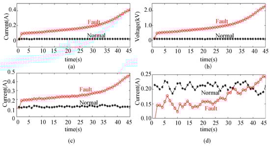
Figure 10.
The 1s time window average RMS value of TSF characteristic quantity. (a) Average current value of fault point, (b) average voltage value of fault point, (c) average value of differential current at the head and tail ends, and (d) average value of zero-sequence current.
In the figure, the average value of zero-sequence voltage continues to increase, showing a consistent trend with the fault current, which can be used as a fault feature of the TSF. However, there are still significant fluctuations in the current signal. Considering that there may be interference signals from other frequency bands in the line, the current waveform is processed using the fast Fourier transform (FFT) algorithm with a unit of 1 s, which is based on the discrete Fourier transform (DFT) [17]. And the signal amplitude near the power frequency is extracted, as shown in Figure 11.
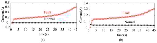
Figure 11.
The amplitude of the power-frequency component of TSF current characteristic quantity: (a) amplitude of differential current power-frequency component, and (b) amplitude of zero-sequence current power-frequency component.
To sum up, taking 1 s as the unit, calculating the average value of the RMS value of the zero-sequence voltage, extracting the amplitude of the power-frequency component of the differential current and the zero-sequence current, the obtained average value of the zero-sequence voltage, the amplitude of the power-frequency component of the differential current, and the amplitude of the power-frequency component of the zero-sequence current are consistent with the variation trend of the fault current and can be used as the TSF characteristic quantities to assist fault identification.
Comparing the three characteristic quantities mentioned above, it is obvious that the average value of zero-sequence voltage and the amplitude of the differential current power-frequency component reflect the trend of fault current change better, while the amplitude of the zero-sequence current power-frequency component reflects the effect of fault current less well. This is due to the fact that the zero-sequence current is easily affected by the ground potential shift or line inrush current, and the accuracy and variable ratio of the through-core current transformer used in this experiment is low. Most lines do not have current transformers installed at the beginning and end of the line, so it is impossible to collect differential current signals. Therefore, the optimal choice for identifying the TSF should be zero-sequence voltage signals. However, if only zero-sequence voltage is used to identify faults, there may be misjudgments when there is an imbalance load or overvoltage on the line. Moreover, when the TSF occurs, the zero-sequence voltage will change for all outgoing lines on the same busbar, making it impossible to specifically distinguish the faulty line. Therefore, current signals are needed to cooperate.
The amplitude of the differential current power-frequency component reflects the effect of fault current changes better than the zero-sequence current. Moreover, due to the need to simultaneously measure the current signals at the head and tail ends of the line for the differential current, the noise interference on the line can be eliminated by subtracting the two current signals. However, it requires a high installation cost to install current transformers at both ends of the line. Therefore, it is recommended to install current transformers at both ends of the line with a high TSF risk for auxiliary identification through differential current. In areas with a low TSF risk, only the zero-sequence current can be used for auxiliary identification.
It can be seen that the average value of the zero-sequence voltage, power-frequency component of the differential current, and power-frequency component of the zero-sequence current can effectively reflect the increasing trend of the fault current and can be used as TSF feature quantities. However, the TSF fault situation varies with parameters such as the length, thickness, and type of tree branches, so it is necessary to explore whether the above data can reflect the changing trend of the fault current in various scenarios. The experimental results for tree branches of different lengths, thicknesses, and types will be analyzed in the following sections.
4.2. Analysis of Tree Characteristics with Different Lengths
The experimental results of branches with numbers 2, 3, and 4 were used to compare the influence of length parameters. The above branches were all pine trees with similar diameters and lengths of 95 cm, 83 cm, and 72 cm, respectively. The same method was used to extract the above fault feature quantities, and the results are shown in Figure 12.
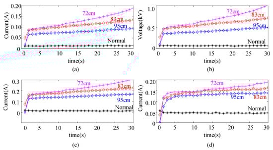
Figure 12.
TSF characteristic quantity of trees with different lengths. (a) Mean value of current at the fault point, (b) average value of zero-sequence voltage, (c) amplitude of differential current power-frequency component, and (d) amplitude of zero-sequence current power-frequency component.
Figure 12 shows that the longer the branch length, the lower the branch fault current. This result is mainly related to the tree resistance. Ignoring the uncertainty in the content and distribution of various substances inside the tree, assuming that the branch is a standard cylinder and the current flows uniformly along the axis through any cross-section of the vegetation, the calculation formula for the initial resistance of the branch is [18]:
In this equation, R is the initial resistance of the tree, r is the radius of the tree, L is the length of the tree, and ρ is the resistivity of the tree. For branches of the same type and similar thickness, the resistivity and branch radius can be considered to be approximately equal. At this point, the longer the branch length, the greater the resistance and the smaller the current, consistent with experimental results.
The variation trends of the average zero-sequence voltage, the amplitude of the differential current power-frequency component, and the amplitude of the zero-sequence current power-frequency component in Figure 12 are consistent with the above analysis, indicating that for branches of different lengths, the above signals can be used as TSF features.
4.3. Analysis of Characteristic Quantities of Trees with Different Diameters
The experimental results of branches with numbers 4, 5, and 6 were used to compare the influence of diameter parameters. The diameters of the above branches were 26.54 mm, 17.16 mm, and 11.70 mm, respectively, with other parameters being consistent. The same method was used to extract the above fault feature quantities, and the results are shown in Figure 13.
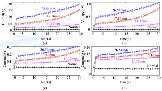
Figure 13.
TSF characteristic quantity of trees with different diameters. (a) Average current value of fault point, (b) average value of zero-sequence voltage, (c) amplitude of differential current power-frequency component, and (d) amplitude of zero-sequence current power-frequency component.
According to Equation (4), the thicker the branch, the larger its cross-sectional area, the lower the resistance, and the higher the fault current. The experimental results in Figure 13 are consistent with this rule. The experimental results are also consistent with current theoretical research.
In Figure 13d, the zero-sequence current initially shows a large value, which may be due to noise interference. In actual distribution networks, the development time of the TSF is longer, and this issue does not occur. Based on the experimental results in Figure 13, for different tree branch diameters, the average value of zero-sequence voltage, the amplitude of differential current power-frequency component, and the amplitude of zero-sequence current power-frequency component still exhibit the same trend as the fault current.
4.4. Analysis of Characteristic Quantities of Different Types of Trees
The experiment results of branches with numbers 1, 5, and 7 were compared based on their types. The types of branches were Bougainvillea, Pine, and Cinnamomum Burmannii. Except for the different types, the other parameters were similar. The experimental results were processed, and the RMS value of zero-sequence voltage, the amplitude of differential current power-frequency component, and the amplitude of zero-sequence current power-frequency component were calculated in units of 1s. The results are shown in Figure 14. It can be seen that the fault development of Bauhinia is faster, while Cinnamomum japonicum and pine are slower.
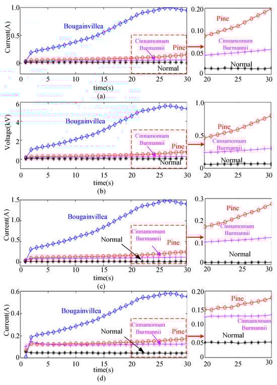
Figure 14.
TSF characteristic quantity of trees of different types. (a) Average current value of fault point, (b) average value of zero-sequence voltage, (c) amplitude of differential current power-frequency component, and (d) amplitude of zero-sequence current power-frequency component.
The enlarged cross-section of the Bougainvillea, Pine, and Cinnamomum Burmannii branches is shown in Figure 15. From Figure 15, it can be seen that the structure of the Bauhinia is more porous, with larger pore diameters on the order of mm, and the center is a through-hole, while the structure of Cinnamomum camphora and pine is more dense, with some pores in the trunk with a diameter on the order of 10–100 μm. Considering that the gas breakdown voltage is much lower than that of solids and liquids, gas discharge is more likely to occur inside loose and porous Bougainvillea, forming an arc channel. Therefore, the equivalent length of trees through which the current passes is relatively smaller, the fault current is larger, the temperature rises faster, and its resistance decreases faster [8], so the fault develops faster. In contrast, the denser Pine and Cinnamomum Burmannii trees have a longer equivalent length of the current channel during the TSF process, resulting in higher resistance and a lower fault current, as well as slower temperature rise, leading to relatively slower development of the fault.
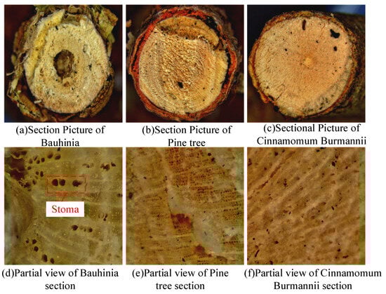
Figure 15.
Sectional picture of trees. (a) Section picture of Bauhinia, (b) section picture of pine tree, (c) sectional picture of Cinnamomum burmannii, (d) partial view of Bauhinia section, (e) partial view of pine tree section, and (f) partial view of Cinnamomum burmannii section.
In summary, the variation trends of the average zero-sequence voltage, the amplitude of the differential current power-frequency component, and the amplitude of the zero-sequence current power-frequency component in Figure 14 are consistent with the above analysis, indicating that for different types of tree branches, the above signals can be used as TSF characteristic quantities.
5. Conclusions
Based on a simulation experiment platform, this study analyzes the trends of typical parameters such as zero-sequence voltage, zero-sequence current, and differential current at the head and tail of the fault phase as the fault progresses in an overhead conductor single-phase tree-to-ground fault. By processing the above data, the TSF feature quantity is obtained, and the following conclusions are drawn:
- (1)
- In the case of a tree-contact single-phase-to-ground fault, as the fault develops, the fault current will gradually increase, and the zero-sequence voltage, zero-sequence current, and differential current at the beginning and end of the faulted phase of the faulted line will also increase accordingly. Considering the small fault current of the TSF, the changing trend of the above characteristic quantities can be used for fault identification;
- (2)
- The average value of the RMS value of the zero-sequence voltage, the amplitude of the power-frequency component of the zero-sequence current, and the amplitude of the power-frequency component of the differential current can reflect the trend of fault current changes and can be used as TSF feature quantities for TSF detection and identification;
- (3)
- The length, diameter, and type of trees significantly affect the fault characteristics of the TSF. For branches of different lengths, diameters, and types, the average value of the RMS value of zero-sequence voltage, the amplitude of the power-frequency component of zero-sequence current, and the amplitude of the power-frequency component of differential current accurately reflect the development trend of the fault. Therefore, the above-mentioned characteristic quantities are applicable to a variety of fault scenarios;
- (4)
- Installing current transformers at the beginning and end of lines with a high TSF risk can identify the TSF through the average value of zero-sequence voltage and the amplitude of differential current power-frequency components. In areas with low TSF risk, TSF identification can be performed using the average value of zero-sequence voltage and the amplitude of zero-sequence current power-frequency components.
Author Contributions
Theoretical analysis, experimental operation and writing original manuscript, J.H., Y.Z. and Y.L.; data analysis and visualization, G.Z. and H.S.; data validation and type setting, J.L.; project administration, writing review, W.N. All authors have read and agreed to the published version of the manuscript.
Funding
This work was supported by a Science and Technology Project of Lijiang Power Supply Bureau, Yunnan Power Grid Co., Ltd. (NO:YNKJXM20222421).
Data Availability Statement
Data is contained within the article.
Conflicts of Interest
The authors declare no conflict of interest.
References
- Han, Z.; Geng, G.; Yan, Z.; Chen, X. Economic Loss Assessment and Spatial–Temporal Distribution Characteristics of Forest Fires: Empirical Evidence from China. Forests 2022, 13, 1988. [Google Scholar] [CrossRef]
- Zhang, J.; Bian, H.; Zhao, H.; Wang, X.; Zhang, L.; Bai, Y. Bayesian Network-Based Risk Assessment of Single-Phase Grounding Accidents of Power Transmission Lines. Int. J. Environ. Res. Public Health 2020, 17, 1841. [Google Scholar] [CrossRef] [PubMed]
- Hurteau, M.D.; Westerling, A.L.; Wiedinmyer, C.; Bryant, B.P. Projected Effects of Climate and Development on California Wildfire Emissions through 2100. Environ. Sci. Technol. 2014, 48, 2298–2304. [Google Scholar] [CrossRef] [PubMed]
- Mitchell, J.W. Power line failures and catastrophic wildfires under extreme weather conditions. Eng. Fail. Anal. 2013, 35, 726–735. [Google Scholar] [CrossRef]
- Short, K.C. A spatial database of wildfires in the United States, 1992–2011. Earth Syst. Sci. Data 2014, 6, 1–27. [Google Scholar] [CrossRef]
- Tian, Y.; Wu, Z.; Li, M.; Wang, B.; Zhang, X. Forest Fire Spread Monitoring and Vegetation Dynamics Detection Based on Multi-Source Remote Sensing Images. Remote Sens. 2022, 14, 4431. [Google Scholar] [CrossRef]
- Zhang, X.; Gui, K.; Liao, T.; Li, Y.; Wang, X.; Zhang, X.; Ning, H.; Liu, W.; Xu, J. Three-dimensional spatiotemporal evolution of wildfire-induced smoke aerosols: A case study from Liangshan, Southwest China. Sci. Total Environ. 2021, 762, 144586. [Google Scholar] [CrossRef] [PubMed]
- Santos, W.; Lopes, F.; Brito, N.; Souza, B. High-impedance fault identification on distribution networks. IEEE Trans. Power Deliv. 2016, 32, 23–32. [Google Scholar] [CrossRef]
- Gomes, D.P.; Ozansoy, C.; Ulhaq, A. High-sensitivity vegetation high-impedance fault detection based on signal’s high-frequency contents. IEEE Trans. Instrum. Meas. 2018, 33, 1398–1407. [Google Scholar] [CrossRef]
- Rai, K.; Hojatpanah, F.; Ajaei, F.B.; Grolinger, K. Deep learning for high-impedance fault detection: Convolutional autoencoders. Energies 2021, 14, 3623. [Google Scholar] [CrossRef]
- Soheili, A.; Sadeh, J. Evidential reasoning based approach to high impedance fault detection in power distribution systems. Transm. Distrib. 2017, 11, 1325–1336. [Google Scholar] [CrossRef]
- Wischkaemper, J.A.; Benner, C.L.; Russell, B.D. Electrical characterization of vegetation contacts with distribution conductors-investigation of progressive fault behavior, 2008 IEEE/PES Transmission and Distribution Conference and Exposition. IEEE Trans. Power Deliv. 2008, 25, 2435–2447. [Google Scholar]
- Gomes, D.P.S.; Ozansoy, C.; Ulhaq, A. Vegetation high-impedance faults’ high-frequency signatures via sparse coding. IEEE Trans. Instrum. Meas. 2019, 69, 5233–5242. [Google Scholar] [CrossRef]
- Sedighi, A.-R.; Haghifam, M.-R.; Malik, O. Soft computing applications in high impedance fault detection in distribution systems. Electr. Power Syst. Res. 2005, 76, 136–144. [Google Scholar] [CrossRef]
- Guo, W.; Wen, F.; Liao, Z.; Wei, L.; Xin, J. An analytic model-based approach for power system alarm processing employing temporal constraint network. IEEE Trans. Power Deliv. 2009, 25, 2435–2447. [Google Scholar] [CrossRef]
- Mujović, S.; Vujošević, S. Method for estimation of location of the asymmetrical phase-to-ground faults existing during an overhead line energisation. IET Sci. Meas. Technol. 2018, 12, 237–246. [Google Scholar] [CrossRef]
- Oberst, U. The Fast Fourier Transform. SIAM J. Control. Optim. 2007, 46, 496–540. [Google Scholar] [CrossRef]
- Djuric, M.; Radojevic, Z.; Terzija, V. Time domain solution of fault distance estimation and arcing faults detection on overhead lines. IEEE Trans. Power Deliv. 1999, 14, 60–67. [Google Scholar] [CrossRef]
Disclaimer/Publisher’s Note: The statements, opinions and data contained in all publications are solely those of the individual author(s) and contributor(s) and not of MDPI and/or the editor(s). MDPI and/or the editor(s) disclaim responsibility for any injury to people or property resulting from any ideas, methods, instructions or products referred to in the content. |
© 2023 by the authors. Licensee MDPI, Basel, Switzerland. This article is an open access article distributed under the terms and conditions of the Creative Commons Attribution (CC BY) license (https://creativecommons.org/licenses/by/4.0/).