Investigations of Flow Boiling in Mini-Channels: Heat Transfer Calculations with Temperature Uncertainty Analyses

Abstract

The article aims to explore boiling heat transfer in mini-channels with a rectangular cross-section using various fluids (HFE-649, HFE-7000, HFE-7100, and HFE-7200). Temperature measurements were conducted using infrared thermography for the heated wall and K-type thermocouples for the working fluid. The 2D mathematical model for heat transfer in the test section was proposed. Local heat transfer coefficients between the heated wall and the working fluid were determined from the Robin condition. The problem was solved by means of the finite element method (FEM) with Trefftz functions. The values of the heat transfer coefficient that were obtained were compared with the results calculated from Newton’s law of cooling. The average relative differences between the obtained results did not exceed 4%. The study included uncertainty analyses for temperature measurements with K- and T-type thermocouples. Expanded uncertainties were calculated using the uncertainty propagation and Monte Carlo methods. Precisely determining the uncertainties in contact temperature measurements is crucial to ensure accurate temperature data for subsequent heat transfer calculations. The results of the heat transfer investigations were compared in terms of fluid temperature, heat transfer coefficients, and boiling curves. HFE-7200 consistently exhibited the highest fluid temperature and temperature differences at boiling incipience, while HFE-7000 demonstrated the highest heat transfer coefficients. HFE-649 showed the lowest heat transfer coefficients. The boiling curves exhibited a typical shape, with a notable occurrence of ‘nucleation hysteresis phenomena’. Upon the analysis of two-phase flow patterns, bubbly and bubbly-slug structures were observed.

1. Introduction

Due to rapid technological development and the demand for compact miniature devices, there have been significant concerns with finding a solution to increase the dissipation of heat. Widespread experimental and theoretical studies are vital for investigating the boiling phenomena in mini-channels. Phase changes that accompany boiling processes allow for the highest possible heat fluxes at low-temperature differences between the heated surface and the working fluid over a small heat transfer area. It is important to determine the conditions under which the flow boiling heat transfer is most intense. The value of the heat transfer coefficient, which describes the intensity of heat transfer during heat transfer by convection, depends on the thermal and flow parameters, the roughness of the heated surface, channel geometry, channel spatial orientation, and the physical properties of the boiling liquid. The heat transfer results concerning flow boiling in mini-channels reported in the literature are inconsistent. The essential element in heat transfer investigations are temperature measurement. The identification of the two-phase flow patterns that occur during the boiling process is often important.

In numerous experimental studies on heat transfer during fluid flow in channels, temperature measurements of the flowing medium are essential. Various methods of temperature measurement can be found in the literature. The main classification covers contact and contactless methods, which are necessary for the temperature measurements of a medium (working fluid) and the temperature of the mini-channels walls.

In most heat transfer investigations, the contact temperature method is utilised with thermoelements. The study described in [1] focused on heat transfer during flow, with the R448A fluid as an environmentally friendly alternative to R404A in commercial refrigeration. The examination covered flow boiling heat transfer and pressure drop in a mini-channel tube while analysing the impact of tube geometry. The results demonstrated promising performance, highlighting the positive influence of mass flux on heat transfer. In addition, it provided a new correlation for predicting the heat transfer coefficient. The authors also explored the thermocouple calibration process before installation, achieving precision within ±0.1 K. The temperature measurements during the experiments involved visually comparing the thermocouple temperatures displayed on the computer monitor with the expected values in the adiabatic test or comparing the temperature readings between the resistance temperature sensors (RTDs) and the thermocouples in the no-flow test (no refrigerant circulation). The checks revealed fluctuations within ±0.15 K of the expected values for the latter or values that fall between the inlet and outlet of the two-path RTDs for the former.

In [2], an experiment studied the two-phase heat transfer and pressure drop of R448A in a 6.0 mm stainless steel tube, analysing the impact of operating parameters such as mass flux and saturation temperature. The primary objective was to determine the heat transfer coefficient. The results were compared with the literature, revealing an assessment of the agreement between the experimental database and selected prediction methods for the two-phase boiling heat transfer coefficient and the frictional pressure drop through statistical analysis. In the investigation, four thermocouples at the top, bottom, left, and right sides of the test tube were calibrated using a thermostatic bath and a reference precision RTD (±0.06 °C), resulting in an overall uncertainty of ±0.10 °C.

The study described in [3] focuses on the experimental investigation of HFE-7100 flow boiling heat transfer within a vertical rectangular mini-channel measuring 1 mm in depth, 30 mm in width, and 120 mm in length. The experimental setup consists of an aluminium block with three lines of five K-type thermocouples positioned along the flow. The main objectives of the experiment include determining the heat transfer coefficient, characterising the flow regimes, and examining the phenomenon of dryness. A comparison was made between the results obtained from an unmodified reference surface and two biphilic surfaces with coating techniques. The local heat transfer coefficient is calculated using a 2D inverse heat conduction method, employing the finite difference method (FDM) for spatial discretisation and Tikhonov’s method for regularisation. The results indicate the minimal sensitivity of mass flux to the heat transfer coefficient, with a prevalence of nucleate boiling. On the contrary, there was significant sensitivity of mass flux to the occurrence of dry-out. The authors also quantified and discussed the impact of two biphilic surface coating techniques on both the boiling and dry-out processes. The SiOC deposition had a relatively small effect on the heat transfer coefficient and the appearance of dry-out compared to that of the reference plate. However, the porous surface coating increased the critical heat flux and improved the transfer in the aluminium area. The authors conclude that the tested biphilic structuration could be optimised for enhanced performance.

In the examination designated in [4], the authors presented the findings on the flow boiling heat transfer characteristics of an R32–oil mixture within a micro-fin tube through experimental investigations. The experimental setup for the flow boiling heat transfer of the R32–oil mixture inside a micro-fin tube included the use of T-type thermocouples to measure fluid temperature. The straight copper micro-fin tube, with an outside diameter of 7.0 mm and an effective heating length of 1000 ± 2.0 mm, was the essential element of the test section. Nine T-type thermocouples were attached to the top, middle, and bottom of the test tube in the gaps. The authors stated that T-type thermocouples have a precision of ±0.2 °C. The investigations involved the observation of flow patterns, the creation of a flow pattern map, and the determination of heat transfer coefficients. Additionally, a new heat transfer correlation was proposed.

In the study outlined in [5], an experimental investigation was carried out to examine the flow boiling heat transfer of R245fa in a circular small tube. The test section consisted of a smooth horizontal stainless-steel tube with an inner diameter of 10 mm and a length of 1.5 m. Direct current was used to heat the tube, and the temperatures of the working fluid temperatures at the inlet and the outlet of the test section were measured using two platinum-resistance thermometers. Furthermore, the outer wall temperature was measured by 24 K-type thermocouples arranged in eight groups of three, evenly spaced at intervals of 190 mm along the test section. The analysis focused on assessing the impacts of vapour quality, mass flux, and evaporating temperature on the flow boiling heat transfer coefficient. A comparative analysis was conducted between the experimental heat transfer coefficients and those predicted using five heat transfer coefficient correlations. The results revealed that the correlation developed by Gungor and Winterton provided the best fit to the experimental data. Based on their work, an improved heat transfer coefficient was proposed.

In the investigations reported in [6], the authors investigated the impact of condenser tube inclination in a passive containment cooling system for nuclear safety. The experiment involved the use of three types of thermocouples, namely N, T, and K. It is important to note that each type of thermocouple has its specific error in temperature measurement.

The primary focus of [7] was the investigation of the impact of various thermocouple constructions on hot spot temperatures. A modelling approach employing finite element analysis was employed to quantitatively assess temperature differences. The main interests included the K, T, and J-type thermocouples, the length of uninsulated wire length, various insulation materials, the thickness of the insulation, and the diameter of the hot spot. Specifically, thermocouples operating in a high-intensity heating zone of around 400 W/(m²K) were found to yield consistently reliable results over time despite practical geometric variations at the hot spot. An evaluation of the impact of different heat transfer coefficients revealed that a lower heat transfer coefficient led to a slower temperature response. Higher heat transfer coefficients generally resulted in less significant temperature deviations, while lower coefficients were associated with higher temperature differences between different constructions.

A technique for measuring the surface temperature of small devices using infrared technology was presented in [8]. The method involved compensating for background radiation by adjusting the temperature to match the measured temperature of the object’s surface. This process was achieved by recording the infrared data against a background regulated to a specific temperature by a thermostat. By using infrared measurements, the study investigated the average and local heat transfer coefficients in a small tube with a 1.07 mm inner diameter under laminar flow conditions. The results revealed lower heat transfer coefficient values compared to the values theoretically predicted for laminar flow, which were obtained for tubes of a larger diameter.

The authors of the study [9] focused on the experimental and numerical investigation of pulsating flows within a rectangular mini-channel subjected to asymmetric sinusoidal flow pulsation patterns. The mini-channel configuration incorporated a heated bottom section treated as a constant heat flux boundary through the uniform heating of the thin foil. Infrared thermography was used for the thermal assessment of the heated boundary in the hydrodynamically and thermally developed region of the mini-channel. A 3D conjugate heat transfer model using ANSYS CFX (https://www.ansys.com/products/fluids/ansys-cfx) was applied for simulations. In the main findings, the authors indicated that the use of a high pulsation flow rate amplitude resulted in an approximately 11% improvement in heat transfer compared to the corresponding steady flow conditions.

In [10], comprehensive PIV (particle image velocimetry) and IRT (infrared thermography) measurements were conducted to investigate the local and overall hydrothermal efficiency in a serpentine heat exchanger featuring separated curved ribs.

Among the contactless methods, liquid crystals deserve mention. In [11], Hożejowska et al. conducted an experimental study and numerical modelling of temperature fields during flow boiling in rectangular mini-channels. The single mini-channel in the test section had a depth of 0.5, 1.0, or 1.5 mm, a width of 20 mm, and a length of 360 mm. Fluorinert FC-72 was the working fluid. Throughout the experiment, a two-dimensional temperature distribution was recorded on the external surface of the heating wall, along with a two-phase flow pattern through an opposite adiabatic transparent wall. Heat transfer calculations for flow boiling utilised a model based on the Trefftz method [12]. The numerical procedure addressed the inverse problems in the heating wall and fluid foil. Two-dimensional temperature distributions, which were found by measuring the outer heated foil surface, were calculated in the fluid in mini-channels. This was coupled with the determination of the void fraction based on the analysis of the two-phase flow pattern.

Regarding heat transfer issues, temperature readings are used to estimate various parameters. The uncertainty of temperature associated with the recorded temperature largely determines the reliability of the values of these parameters. According to the recommendations of the guide [13], the Monte Carlo (MC) method is indicated to be used to determine the uncertainty of the measurement. In [14], the MC method was used to assess the uncertainty of thermocouple calibration between temperature-fixed points using a polynomial interpolation defined by the calibration data. The results were compared with the uncertainty calculated using the classical method based on the law of propagation of uncertainty [15].

The authors of [16] deal with the application of the Monte Carlo method for uncertainty quantification in temperature measurements in an experimental model of heat transfer that describes the behaviour of a homogeneous, isotropic, and linear solid.

The work in [17] is concerned with the experimental determination of the thermal conductivity of nylon 66 based on the measurement of the temperature due to K-type thermocouples. The uncertainty of the determined value was assessed using the Monte Carlo method.

In [18], the researchers performed transient heat transfer experiments using liquid crystal thermography to assess the uncertainty of local measurements using the MC method. This methodology obtained lower and upper boundaries for a confidence interval at a specified confidence level for the heat transfer coefficient, calculated locally for individual pixels. The local uncertainty measurement was compared to the conventional error propagation technique. Such a comparison highlighted the benefits of accounting for nonlinearity and local uncertainty in peak detection. The MC method was also used in [19] to propose an uncertainty budget to determine the uncertainty of the post-error compensation of measurement systems. While analysing the results, the authors proposed strategies to mitigate the uncertainty of the final measurement.

The sensitivities of each individual component can be determined using the GUM approach [15] for the estimation of uncertainty. Furthermore, a complete uncertainty budget for measurements is often used for a clear presentation of the data. For example, this approach was applied in [20] to determine the uncertainty in the measurements of ambient mercury vapour. The next example is the uncertainty budget provided in [21] to determine the geometric properties of an optical measurement system and to verify compliance with specific task tolerances according to ISO 14253–1 [22].

The primary objective of this study is to investigate boiling heat transfer during flow of cooling fluid in mini-channels, based on data collected from experiments. Recognising the significant impact of temperature measurement specifications on heat transfer results and noting the absence of a thorough analysis in the existing literature, the work includes a detailed examination of uncertainty analyses for temperature measurements obtained from K- and T-type thermocouples. Expanded uncertainties were calculated using both the uncertainty propagation method and the Monte Carlo method for comparison. A 2D mathematical model for heat transfer in the test section with mini-channels was formulated, determining local heat transfer coefficients between the heated wall and the working fluid from the Robin condition. The problem was solved using the finite element method (FEM) with Trefftz functions.

The novelty of this study lies in its experimental approach to improving the precision of temperature measurements, especially in terms of reducing uncertainties. The primary objective is to investigate the phenomena occurring during flow boiling in mini-channels. The study involves analysing fluid temperatures, heat transfer coefficients and their distributions, and exploring the course of boiling curves. One specific aspect that the study aims to explore is the ‘nucleation hysteresis’ phenomenon in various cooling fluids commonly used in technological devices. The outcomes of these investigations are expected to contribute to better temperature control in devices that undergo a phase change in their working fluid during operation.

The overarching goal is to gain a better understanding of the boiling phenomenon, which is deemed crucial for achieving improved temperature control in devices that undergo phase changes. The study emphasises the significance of this understanding in both scientific and technological contexts.

2. Temperature Uncertainty Analyses

2.1. Main Goal

In studies on boiling heat transfer during flow in mini-channels, as described in Section 3, precise temperature measurement is crucial. It should be underlined that the determination of the heat transfer coefficient is based on fluid temperature data collected during experiments. The temperature of the working fluid was measured due to K-type thermocouples that co-operated with data acquisition stations. The uncertainty of the determined heat transfer coefficient is also strongly dependent on the accuracy of the fluid temperature measurement. The overall aim of the next thermometry study was to determine the uncertainty of the entire measurement path that involved the measurement of the temperature of the working fluid. Additionally, the use of another type of thermocouple, which has higher nominal measurement uncertainties according to current standards (T-type thermocouples), was investigated for comparison.

The additional experimental setup, dedicated to estimating the uncertainty in the path for working fluid temperature measurement, is designed considering the authors’ explained additional purpose. This chapter aims to examine the results of experimental investigations related to temperature measurement using thermoelectric sensors with compensating cables. The setup was additionally equipped with thermometers, one of which functioned as the data acquisition system.

2.2. Experimental Stand

Figure 1 illustrates the measuring equipment used for the experiment that led to the comparative study of contact temperature sensors. In Figure 1a, the connections between the main apparatus are depicted, while Figure 1b provides a photo of the setup. The CDT9100-ZERO dry-well calibrator (1) served as a source of constant reference temperature for the contact sensors being compared. The highly precise temperature measurement instrument (thermometer) (type STA 510 DT (PRESYS)), in collaboration with the resistance temperature sensor (Pt-100 1/5 DIN B) [23], acted as a laboratory reference temperature standard and served as the data acquisition station. An additional Pt-100 class A resistance temperature sensor, paired with the EMT-55 thermometer (3) (Czaki Thermo-Product, Raszyn-Rybie, Poland), functioned as an auxiliary standard. An additional LB 532 (LAB-EL, Reguly/Warsaw, Poland) recorded information on the physical conditions of the ambient air in the laboratory.

All measuring instruments, which were powered by 230 V, were connected to the electrical supply through the automatic voltage regulator, type DLT SRV SO-HO 15 KVA (Delta Elektrik Elektronik, Istanbul, Turkey).

During the experimental sets, the thermocouples T-type and K-type were sequentially connected to the temperature measurement instrument (2). They were used to measure the temperature in the calibration bore of the temperature dry-well calibrator (1). A PC (4) equipped with specialist software was applied for data acquisition.

Figure 1. Experimental setup for temperature uncertainty analyses: (a) schematic diagram; (b) photo; 1—dry-well temperature calibrator, model CDT9100-ZERO (WIKA Polska, Wloclawek, Poland); 2—temperature measurement instrument, model STA 510 DT (PRESYS, Sao Paulo, Brazil), serving as data acquisition station; 3—thermometer, model EMT-55 (Czaki Thermo-Product), 4—PC with software.

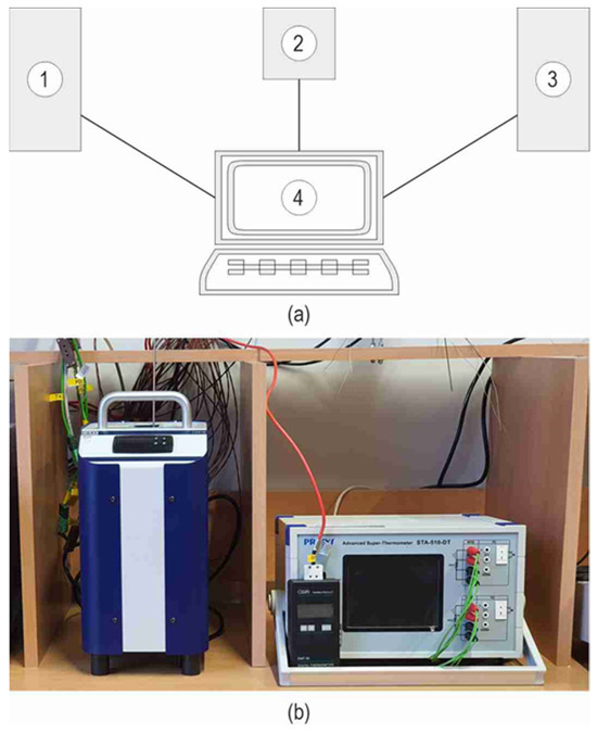
Figure 1. Experimental setup for temperature uncertainty analyses: (a) schematic diagram; (b) photo; 1—dry-well temperature calibrator, model CDT9100-ZERO (WIKA Polska, Wloclawek, Poland); 2—temperature measurement instrument, model STA 510 DT (PRESYS, Sao Paulo, Brazil), serving as data acquisition station; 3—thermometer, model EMT-55 (Czaki Thermo-Product), 4—PC with software.

2.3. Experimental Procedure

Simultaneous experiments were carried out using the dry-well temperature calibrator model CDT9100-ZERO (WIKA), recognised for its precision of ±0.05° C at 0 °C temperature [24]. Six thermocouples were placed in the dry measuring bore of the temperature calibrator, including three K-type and four T-type. Each thermocouple was equipped with a 0.5 m long compensating cable. The certified Pt-100 1/5 DIN B resistance temperature sensor (PRESYS) [25] served as a laboratory reference for temperature measurement [26]. This sensor was connected to a channel of the STA 510 DT (PRESYS) temperature measurement instrument [27], while the sequentially tested thermocouples were connected to the second channel. Temperature measurements were conducted simultaneously using an additional Pt-100 class A resistance temperature sensor working in collaboration with the EMT-55 thermometer (Czaki Thermo-Product). The experiments involved incrementally increasing the temperature ($T_{kz}$) every 20 °C within the range of 0 to 100 °C on the temperature calibrator. Basic data regarding the measurement conditions were directly recorded on the STA 510 DT instrument.

Statistical computational methods for type A standard measurement uncertainty calculation were employed for the analysis of the results. Additionally, the uncertainty was calculated using the Monte Carlo method (MC), following the recommendations outlined in the guide [13].

Empirical cumulative distribution functions of the output quantities were determined based on the assumed probability distributions of the input variables. The quantiles calculated at the 0.025 and 0.975 levels represented the confidence interval boundaries for the output quantities at a confidence level of 0.95. The uncertainty obtained from the MC simulation was compared with the expanded uncertainty obtained through uncertainty propagation [15]. Both calculation methods yielded similar results.

The following conditions prevailed in the laboratory during the experiment: the temperature varied in the range from 20.9 to 21.1 °C (since the error caused by the stability of the ambient temperature during the time of measurement denoted by ${\mathsf{\delta }T}_s$ is equal to 0.2 °C), the relative humidity was 31% RH and the atmospheric pressure was 998 hPa [28].

2.4. Main Statistical Parameters Related to the Experimental Data

It should be emphasised that the objective was to determine the expanded uncertainty for the measurement paths used to measure the temperature of the working fluid at the inlet and outlet of the mini-channels constituting the test section, which is an essential element of the experimental setup used for investigations of heat transfer with a change of phase during fluid flow in mini-channels. Furthermore, instead of K-type thermocouples (see Section 4), T-type thermocouples were tested for comparison.

Two K-type thermocouples, designated ${\mathrm{T}\mathrm{C}}_{\mathrm{K}1}$ and ${\mathrm{T}\mathrm{C}}_{\mathrm{K}2}$, were used to monitor the working fluid during the heat transfer experiment. These thermocouples were mounted on the inlet and outlet collectors of the test section. Additional K-type thermocouples, named ${\mathrm{T}\mathrm{C}}_{\mathrm{K}3}$, were tested for comparison.

A modernisation of the experimental setup, where heat transfer experiments are conducted, is planned to achieve improved temperature measurement accuracy. Following the improvement, unsteady-state experiments are premeditated. Therefore, T-type thermocouples (${\mathrm{T}\mathrm{C}}_{\mathrm{T}1},{\mathrm{T}\mathrm{C}}_{\mathrm{T}2}$, and ${\mathrm{T}\mathrm{C}}_{\mathrm{T}3})$ were chosen for statistical analyses of the uncertainty of temperature measurements, taking into account the entire measurement path.

The results of the experimental temperature measurement conducted for K- and T-type thermocouples are illustrated in the form of box plots. The box and whisker plots [29] shown in Figure 2 display the summary of a set of measurement data: minimum ($T_{min}$), first quartile (Q1), median (Me), third quartile (Q3), and maximum ($T_{max})$.

Table 1 shows the selected statistical parameters provided for the examined pairs of thermoelectric sensors (the resistance temperature sensor Pt-100 1/5 DIN B and a tested thermocouple), while the temperature $T_{3z}=40 °$C was set at the temperature calibrator. In addition, the interquartile range (IQR) and the error in the temperature reading by a specified thermocouple are placed in this table.

It could be explained that the interquartile range (IQR) is a statistical measure of the spread of data around the central part of the distribution. Mathematically, IQR is determined by subtracting the first quartile (Q1) from the third quartile (Q3), denoted as ($IQR=\mathrm{Q}3-\mathrm{Q}1$). This measure offers valuable insights into the variability within the middle 50% of the dataset.

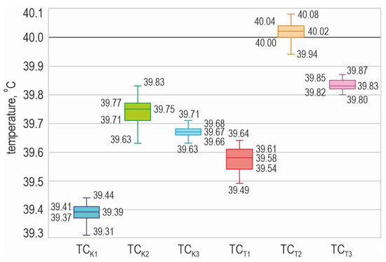
Figure 2. Box and whisker plots for the measurement results conducted for K-type (${\mathrm{T}\mathrm{C}}_{\mathrm{K}1}, {\mathrm{T}\mathrm{C}}_{\mathrm{K}2}$, and ${\mathrm{T}\mathrm{C}}_{\mathrm{K}3}$) and T-type thermocouples, the set point temperature $T_{3z }=40 °$C.

Figure 2. Box and whisker plots for the measurement results conducted for K-type (${\mathrm{T}\mathrm{C}}_{\mathrm{K}1}, {\mathrm{T}\mathrm{C}}_{\mathrm{K}2}$, and ${\mathrm{T}\mathrm{C}}_{\mathrm{K}3}$) and T-type thermocouples, the set point temperature $T_{3z }=40 °$C.

Table 1. The summary of selected statistical parameters for the compared pairs of thermoelectric sensors at the specified temperature $T_{3z}=40 °\mathrm{C}$ set at the temperature calibrator.

${\mathit{T}}_{3\mathit{z}}$ = 40 °C
Statistical Parameters	${\mathbf{T}\mathbf{C}}_{\mathbf{K}1}$	${\mathbf{R}\mathbf{T}\mathbf{D}}_1$	${\mathbf{T}\mathbf{C}}_{\mathbf{K}2}$	${\mathbf{R}\mathbf{T}\mathbf{D}}_1$	${\mathbf{T}\mathbf{C}}_{\mathbf{K}3}$	${\mathbf{R}\mathbf{T}\mathbf{D}}_1$
	°C	°C	°C	°C	°C	°C
$T_{max}$	39.44	40.026	39.83	40.039	39.71	40.033
Q3	39.41	40.019	39.77	40.02	39.68	40.012
Me	39.39	40.011	39.75	40.005	39.67	40.008
$\overline{T}$	39.384	40.011	39.744	40.005	39.67	40.007
Q1	39.37	40.001	39.71	39.991	39.66	39.995
$T_{min}$	39.31	39.995	39.63	39.975	39.63	39.983
$IQR$	0.04	0.018	0.06	0.029	0.02	0.017
${\delta T}_{TC}$	−0.627		−0.261		−0.337
	${\mathbf{T}\mathbf{C}}_{\mathbf{T}1}$	${\mathbf{R}\mathbf{T}\mathbf{D}}_1$	${\mathbf{T}\mathbf{C}}_{\mathbf{T}2}$	${\mathbf{R}\mathbf{T}\mathbf{D}}_1$	${\mathbf{T}\mathbf{C}}_{\mathbf{T}3}$	${\mathbf{R}\mathbf{T}\mathbf{D}}_1$
	°C	°C	°C	°C	°C	°C
$T_{max}$	39.64	40.034	40.08	40.031	39.87	40.033
Q3	39.61	40.014	40.04	40.011	39.85	40.017
Me	39.58	39.9935	40.02	40.004	39.83	40.011
$\overline{T}$	39.576	39.9979	40.02	40.004	39.83	40.011
Q1	39.54	39.984	40.00	39.997	39.82	40.003
$T_{min}$	39.49	39.959	39.94	39.981	39.80	39.984
$IQR$	0.07	0.030	0.04	0.014	0.03	0.014
${\delta T}_{TC}$	−0.4219		0.016		−0.181

where $T_{min}$—is the lowest observed temperature value not deviating from the remaining values, $T_{max}$—is the highest observed temperature value not deviating from the remaining values, $\overline{T}$—average temperature, Me—median temperature, IQR—interquartile range, ${\mathrm{R}\mathrm{T}\mathrm{D}}_1$—the temperature value measured using the PRESYS data acquisition station equipped with the Pt-100 type 1/5 DIN B resistance temperature sensor on the first channel, ${\delta T}_{TC}$—the error in temperature reading by a specified thermocouple; representing the difference between the mean temperature value measured by the investigated thermocouple ${\mathrm{T}\mathrm{C}}_{xx}$ and the mean temperature value measured using the reference resistive sensor ${\mathrm{R}\mathrm{T}\mathrm{D}}_1$.

Table 1. The summary of selected statistical parameters for the compared pairs of thermoelectric sensors at the specified temperature $T_{3z}=40 °\mathrm{C}$ set at the temperature calibrator.

${\mathit{T}}_{3\mathit{z}}$ = 40 °C
Statistical Parameters	${\mathbf{T}\mathbf{C}}_{\mathbf{K}1}$	${\mathbf{R}\mathbf{T}\mathbf{D}}_1$	${\mathbf{T}\mathbf{C}}_{\mathbf{K}2}$	${\mathbf{R}\mathbf{T}\mathbf{D}}_1$	${\mathbf{T}\mathbf{C}}_{\mathbf{K}3}$	${\mathbf{R}\mathbf{T}\mathbf{D}}_1$
	°C	°C	°C	°C	°C	°C
$T_{max}$	39.44	40.026	39.83	40.039	39.71	40.033
Q3	39.41	40.019	39.77	40.02	39.68	40.012
Me	39.39	40.011	39.75	40.005	39.67	40.008
$\overline{T}$	39.384	40.011	39.744	40.005	39.67	40.007
Q1	39.37	40.001	39.71	39.991	39.66	39.995
$T_{min}$	39.31	39.995	39.63	39.975	39.63	39.983
$IQR$	0.04	0.018	0.06	0.029	0.02	0.017
${\delta T}_{TC}$	−0.627		−0.261		−0.337
	${\mathbf{T}\mathbf{C}}_{\mathbf{T}1}$	${\mathbf{R}\mathbf{T}\mathbf{D}}_1$	${\mathbf{T}\mathbf{C}}_{\mathbf{T}2}$	${\mathbf{R}\mathbf{T}\mathbf{D}}_1$	${\mathbf{T}\mathbf{C}}_{\mathbf{T}3}$	${\mathbf{R}\mathbf{T}\mathbf{D}}_1$
	°C	°C	°C	°C	°C	°C
$T_{max}$	39.64	40.034	40.08	40.031	39.87	40.033
Q3	39.61	40.014	40.04	40.011	39.85	40.017
Me	39.58	39.9935	40.02	40.004	39.83	40.011
$\overline{T}$	39.576	39.9979	40.02	40.004	39.83	40.011
Q1	39.54	39.984	40.00	39.997	39.82	40.003
$T_{min}$	39.49	39.959	39.94	39.981	39.80	39.984
$IQR$	0.07	0.030	0.04	0.014	0.03	0.014
${\delta T}_{TC}$	−0.4219		0.016		−0.181

where $T_{min}$—is the lowest observed temperature value not deviating from the remaining values, $T_{max}$—is the highest observed temperature value not deviating from the remaining values, $\overline{T}$—average temperature, Me—median temperature, IQR—interquartile range, ${\mathrm{R}\mathrm{T}\mathrm{D}}_1$—the temperature value measured using the PRESYS data acquisition station equipped with the Pt-100 type 1/5 DIN B resistance temperature sensor on the first channel, ${\delta T}_{TC}$—the error in temperature reading by a specified thermocouple; representing the difference between the mean temperature value measured by the investigated thermocouple ${\mathrm{T}\mathrm{C}}_{xx}$ and the mean temperature value measured using the reference resistive sensor ${\mathrm{R}\mathrm{T}\mathrm{D}}_1$.

When analysing the data presented Table 1, in the case of three pairs of thermoelectrical sensors, namely ${\mathrm{R}\mathrm{T}\mathrm{D}}_1$ with ${\mathrm{T}\mathrm{C}}_{\mathrm{K}3}$, ${\mathrm{R}\mathrm{T}\mathrm{D}}_1$ with ${\mathrm{T}\mathrm{C}}_{\mathrm{T}2}$, and ${\mathrm{R}\mathrm{T}\mathrm{D}}_1$ with ${\mathrm{T}\mathrm{C}}_{\mathrm{T}3}$, it was noticed that the arithmetic mean equals the median, indicating a symmetrical distribution of the temperature measurement results. The minimum interquartile range (IQR) of 0.02 °C was observed for the ${\mathrm{T}\mathrm{C}}_{\mathrm{K}3}$ thermocouple, while a slightly wider IQR of 0.03 °C was found for the ${\mathrm{T}\mathrm{C}}_{\mathrm{T}2}$ thermocouple and ${\mathrm{T}\mathrm{C}}_{\mathrm{T}3}$, with an IQR of 0.04 °C. Additionally, ${\mathrm{T}\mathrm{C}}_{\mathrm{T}3}$ had an IQR of 0.04 °C, making it the third thermocouple in order with the narrowest IQR. This means that the majority of the data are concentrated around the centre of the distribution, directly influencing the value of the standard uncertainty.

Thus, considering only the width of the IQR temperature measurement, thermocouples ${\mathrm{T}\mathrm{C}}_{\mathrm{K}3}$, ${\mathrm{T}\mathrm{C}}_{\mathrm{T}2}, \mathrm{a}\mathrm{n}\mathrm{d} {\mathrm{T}\mathrm{C}}_{\mathrm{T}3}$ are indicated to be used in the modification of the temperature measurement system realised in the experimental setup dedicated for heat transfer research during flow boiling in mini-channels. Furthermore, to achieve higher accuracy in temperature measurement, it is worth mentioning that the smallest error ${\delta T}_{TC}$ is exhibited by the thermocouples ${\mathrm{T}\mathrm{C}}_{\mathrm{T}2}$ and ${\mathrm{T}\mathrm{C}}_{\mathrm{T}3}$, with ${\delta T}_{TC}$ errors of 0.016 °C and −0.181 °C, respectively. It should be emphasised that the knowledge of the error magnitude, ${\delta T}_{TC}$, at a given temperature, allows for its consideration in the calculations of the heat transfer coefficient by applying the appropriate temperature correction.

3. Estimation of the Working Fluid Temperature Measurement

3.1. Procedure for the Uncertainty Estimation of the Temperature Measurement

The procedure for estimating the uncertainty of temperature measurements, dedicated to working fluid temperature measurement in heat transfer research, involved the following steps:

• The estimation of the measurement uncertainty of the data acquisition station;
• The estimation of the uncertainty of the temperature dry-well calibrator;
• The estimation of the uncertainty of the EMT-55 meter with a Pt-100 resistance temperature sensor;
• The estimation of the uncertainty of the tested measurement paths.

3.2. Estimation of the Measurement Uncertainty of the Data Acquisition Station

The STA 510 DT (PRESYS) temperature measurement instrument operates in the experimental setup shown in Figure 1 not only as a precise temperature measurement instrument (thermometer) but also as a data acquisition station. In future heat transfer experiments planned for the setup dedicated to the investigation of flow boiling in mini-channels (as described in Section 4), the STA 510 DT instrument is intended to replace the existing data acquisition station, providing higher accuracy in temperature readings.

Type-B standard uncertainty was estimated for the STA 510 DT (PRESYS) temperature measurement instrument (data acquisition station), according to the manufacturer’s documentation [27]. It was assumed that the accuracy of the readings due to this device is characterised by a rectangular distribution. The calculated standard uncertainty $u\left(T_{DASa}\right)$ and expanded uncertainty $U\left(T_{DASa}\right)$ of this data acquisition station, co-operating with selected thermoelements at specified temperatures, are given in Table 2. Furthermore, the data provided by the manufacturer (accuracy and resolution) concerning temperature measurement are also listed in this table.

The compensation error of the cold end of the thermocouple, ${\delta }_{CJC}$, was assumed to be ±0.1 °C [27], according to rectangular probability distribution. Therefore, the standard uncertainty of the data acquisition station, depending on the value of the compensation error of the cold end of the thermocouple, was given as $u\left(T_{cjc}\right)=\pm 0.029$.

The accuracy (for the typical values, using the coefficients in [30]) for the PRESYS Pt-100 1/5 DIN B resistance temperature sensor, as specified by the manufacturer [27], was ±0.030 °C for the temperature of −38.0 °C, ±0.020 °C for the temperatures 0.0 °C and 232.0 °C, and ±0.030 °C for the temperature of 420.0 °C.

Table 2. The accuracy, resolution, and uncertainties of the temperature measurement results, achieved for selected thermoelements at specified temperatures, with the use of the STA 510 DT (PRESYS) [27].

Thermoelement	Temperature	Accuracy	Resolution	$\mathit{u}\left({\mathit{T}}_{\mathit{D}\mathit{A}\mathit{S}\mathit{a}}\right)$	$\mathit{u}\left({\mathit{T}}_{\mathit{D}\mathit{A}\mathit{S}\mathit{r}}\right)$	$\mathit{u}\left({\mathit{T}}_{\mathit{D}\mathit{A}\mathit{S}}\right)$
	°C	°C	°C	°C	°C	°C
RTD, Pt-100	−38	± 0.01	0.001	0.0058	0.0006	0.030
	420
Thermocouple K-type	0	± 0.04	0.01	0.023	0.0058	0.037
	600
Thermocouple T-type	0	± 0.04	0.01	0.023	0.0058	0.037
	300	± 0.03		0.017	0.0057	0.034

$u\left(T_{DASa}\right)$—standard uncertainty for the error of the data acquisition station accuracy; $u\left(T_{DASr}\right)$—standard uncertainty for the error of the data acquisition station resolution; $u\left(T_{DAS}\right)$—standard uncertainty for the error of the data acquisition station, which is computed as the square root of the sum of the squares of three standard uncertainties: $u\left(T_{DASa}\right)$, $u\left(T_{DASr}\right)$, and $u\left(T_{cjc}\right)$.

Table 2. The accuracy, resolution, and uncertainties of the temperature measurement results, achieved for selected thermoelements at specified temperatures, with the use of the STA 510 DT (PRESYS) [27].

Thermoelement	Temperature	Accuracy	Resolution	$\mathit{u}\left({\mathit{T}}_{\mathit{D}\mathit{A}\mathit{S}\mathit{a}}\right)$	$\mathit{u}\left({\mathit{T}}_{\mathit{D}\mathit{A}\mathit{S}\mathit{r}}\right)$	$\mathit{u}\left({\mathit{T}}_{\mathit{D}\mathit{A}\mathit{S}}\right)$
	°C	°C	°C	°C	°C	°C
RTD, Pt-100	−38	± 0.01	0.001	0.0058	0.0006	0.030
	420
Thermocouple K-type	0	± 0.04	0.01	0.023	0.0058	0.037
	600
Thermocouple T-type	0	± 0.04	0.01	0.023	0.0058	0.037
	300	± 0.03		0.017	0.0057	0.034

$u\left(T_{DASa}\right)$—standard uncertainty for the error of the data acquisition station accuracy; $u\left(T_{DASr}\right)$—standard uncertainty for the error of the data acquisition station resolution; $u\left(T_{DAS}\right)$—standard uncertainty for the error of the data acquisition station, which is computed as the square root of the sum of the squares of three standard uncertainties: $u\left(T_{DASa}\right)$, $u\left(T_{DASr}\right)$, and $u\left(T_{cjc}\right)$.

3.3. Estimation of the Measurement Uncertainty of the Temperature Dry-Well Calibrator

The dry-well temperature calibrator, Wika CDT9100-ZERO (WIKA Polska, Wloclawek, Poland), was used as a stable reference temperature source for comparing the measurements provided by the thermoelectric sensors. The initial procedural step involves establishing the standard uncertainty for a specified $T_{iref}$ (the i-th temperature measured by the laboratory standard, i.e., the STA 510 DT instrument with the Pt-100 type 1/5 DIN B resistance temperature sensor) at the output of the temperature calibrator. This determination comprises summing the following elements:

• $T_{kz}$—the k-th temperature set at the input of the temperature calibrator;
• ${\mathsf{\delta }T}_a$—the accuracy error of the temperature dry-well calibrator, defined as the discrepancy between the measured value and the reference value [24], as derived from the manufacturer’s documentation, which was 0 ± 0.05 °C for 0 °C and 0 ± 0.1 °C for other temperatures;
• ${\mathsf{\delta }T}_v$—the temperature stability error, which is the maximum temperature difference at a stable temperature achieved during the time interval of 30 min, was estimated to be 0 ± 0.05 °C, based on the manufacturer’s documentation [24];
• ${\mathsf{\delta }T}_r$—the temperature calibrator setting resolution error for the built-in temperature dry-well calibrator thermometer was 0.1 °C [24];
• ${\mathsf{\delta }T}_G$—the error related to the axial gradient of the temperature, which takes into account the temperature variation in the metal block of the dry-well calibrator, was assumed to be 0 ± 0.05 °C based on the manufacturer’s documentation [24];
• ${\mathsf{\delta }T}_R$—the error related to the temperature difference in the radial direction in the metal block of the dry-well calibrator (between the built-in thermometer and the working standard) was estimated to be 0 ± 0.10 °C;
• ${\mathsf{\delta }T}_D$—the error resulting from the potential change in the indication of the temperature value of the working standard since its last calibration, caused by the ageing of the material of the resistive sensor, which was estimated to be 0 ± 0.02 °C based on the known properties of the Pt-100-type RTD sensors [31].

In the statistical analysis presented, an uncertainty budget is employed for a systematic and comprehensive assessment of various sources of uncertainty related to measurements or experimental processes. It offers a structured breakdown of the individual contributions to overall uncertainty, aiding in the identification and quantification of factors influencing precision and accuracy. Understanding the reliability and limitations of the obtained results is essential in measurements, and an uncertainty budget plays a crucial role in assessing uncertainties across different components of the measurement setup, thereby impacting the final measurement uncertainty.

The uncertainty budget, describing the temperature measurement uncertainty using the WIKA CDT9100-ZERO calibrator, is systematically formulated to determine the standard uncertainty $u\left(T_{ref}\right)$ following the guidelines specified in [31].

Table 3. Uncertainty budget of temperature measurement ($T_{iref}$) using WIKA CDT-9100-ZERO temperature dry-well calibrator.

Quantities	Estimates	Standard Uncertainty	Probability Distribution	Sensitivity Coefficient	Contribution to Combined Uncertainty
${\mathit{X}}_{\mathit{i}}$	${\mathit{x}}_{\mathit{i}}$	$\mathit{u}\left({\mathit{x}}_{\mathit{i}}\right)$		${\mathit{c}}_{\mathit{i}}$	${\mathit{u}}_{\mathit{i}}$
°C	°C	°C	-	-	°C
$T_{1z}$	0	0.023 [27]	normal	1.0	0.023
$T_{2z}$	20	0.023 [27]	normal	1.0	0.023
$T_{3z}$	40	0.023 [27]	normal	1.0	0.023
$T_{4z}$	60	0.023 [27]	normal	1.0	0.023
$T_{5z}$	80	0.023 [27]	normal	1.0	0.023
$T_{6z}$	100	0.023 [27]	normal	1.0	0.023
${\delta T}_a$ *	0.0	0.029 [24]	rectangular	1.0	0.029
${\delta T}_a$ **	0.0	0.058 [24]	rectangular	1.0	0.058
${\mathsf{\delta }T}_v$	0.0	0.029 [24]	rectangular	1.0	0.029
${\mathsf{\delta }T}_r$	0.0	0.029 [24]	rectangular	1.0	0.029
${\mathsf{\delta }T}_G$	0.0	0.029 [24]	rectangular	1.0	0.029
$\delta T_R$	0.0	0.058 [24]	rectangular	1.0	0.058
${\delta T}_D$	0.0	0.006 [27]	rectangular	1.0	0.006

* = 0 °C; ** = other temperatures set on the temperature dry-well calibrator.

outlines the uncertainty budget for the temperature calibrator, excluding the temperature error due to heat conduction through the sheath of the thermometer since the diameter of the thermocouples under testing was significantly less than 5 mm [31]. The types of probability distributions specified in Table 3 were assumed as follows: rectangular—based on the equipment manufacturer’s documentation [24] or normal—based on the information contained in the calibration certificate [32], particularly with respect to the calibration method employed.

Next, the combined standard uncertainty is determined using the law of propagation of uncertainty [15]. The obtained results are as follows: $u\left(T_{ref}\right)=0.096$ °C for 0 °C and $u\left(T_{ref}\right)=0.108 °\mathrm{C}$ for other temperatures. For a coverage factor equal to 2 (indicating a 95% confidence level), the expanded uncertainty values are $U\left(T_{ref}\right)=0.19 °\mathrm{C}$ for 0 °C and $U\left(T_{ref}\right)=0.21 °\mathrm{C}$ for the remaining temperatures.

3.4. Estimation of the Uncertainty of the EMT-55 Meter with a Pt-100 Resistance Temperature Sensor

According to the calibration certificate [32], the standard uncertainty of the EMT-55 measuring instrument fitted with the resistance temperature sensor Pt-100 class A is $u\left(T_{EMT}\right)=\pm 0.1 °\mathrm{C}$. The estimated standard uncertainty for 0 °C is $u\left(T_{ref}\right)=0.126$ °C, and for other temperatures, u$\left(T_{ref}\right)=0.135$ °C. Assuming a normal distribution, a probability level of 0.95, and a coverage factor k = 2, the expanded uncertainties of temperature measurement were obtained as follows: $U\left(T_{ref}\right)=0.25$ °C for 0 °C, and $U\left(T_{ref}\right)=0.27$ °C for other temperatures. A normal distribution was assumed for the measurement of the reference temperature; hence, ${\delta T}_{ref}=\pm U\left(T_{ref}\right)$.

3.5. Estimation of the Uncertainty of the Tested Measurement Paths

The temperature $T_{ijx}$ (the i-th temperature measured by the j-th thermoelement) measured in the bore of the temperature dry-well calibrator measured by the tested thermocouples was calculated by summing up the following elements:

• $T_{iref}$—the i-th temperature measured in the temperature calibrator (measuring bore);
• ${\delta T}_{jT}$—the error of the j-th thermocouple, assumed to be ±1.5 °C for K-type thermocouples and ±0.5 °C for T-type thermocouples [33];
• ${\delta T}_{ref}$—the error caused by the temperature in the calibration bore in the temperature calibrator, assumed to be ${\delta T}_{ref}=\pm 0.252$ °C for 0 °C and ${\delta T}_{ref}=\pm 0.27$ °C for others temperatures;
• ${ \delta T}_{jK}$—the error of the j-th compensating cables, assumed to be 0 ± 1.5 °C for K-type thermocouples and 0 ± 0.5 °C for T-type thermocouples [34];
• ${\mathsf{\delta }T}_{sl}$—the error caused by the stability of the ambient temperature during the time of measurement, assumed to be 0.2 °C;
• ${\delta T}_{DAS}$—the error of the STA 510 DT (PRESYS) temperature measurement instrument (data acquisition station), assuming a normal distribution, is given by ${\delta T}_{DAS}=2 ·u\left(T_{DAS}\right)=0\pm 0.074 °\mathrm{C}$ for T- and K-type thermocouples (see Table 2).

When using a recently manufactured data acquisition station with an operating time not exceeding 10 h for the experiment, it was assumed that the temperature error caused by long-term temperature drift would be intentionally omitted in further calculations.

Table 4. Uncertainty budget of temperature measurement realised on the tested measurement paths.

Quantities	Estimates	Standard Uncertainty	Probability Distribution	Sensitivity Coefficient	Contribution to Combined Uncertainty
${\mathit{X}}_{\mathit{i}}$	${\mathit{x}}_{\mathit{i}}$	$\mathit{u}\left({\mathit{x}}_{\mathit{i}}\right)$		${\mathit{c}}_{\mathit{i}}$	${\mathit{u}}_{\mathit{i}}$
°C	°C	°C	-	-	°C
${\delta T}_{ref}$ *	0.0	0.126	normal	1.0	0.126
${\delta T}_{ref}$ **	0.0	0.135	normal	1.0	0.135
${\delta T}_{jT}$^	0.0	0.866 [33]	rectangular	1.0	0.866
${\delta T}_{jT}$^^	0.0	0.289 [33]	rectangular	1.0	0.289
${\mathsf{\delta }T}_s$	0.0	0.058	rectangular	1.0	0.058
${\mathsf{\delta }T}_{jK}$^	0.0	0.866 [34]	rectangular	1.0	0.866
${\mathsf{\delta }T}_{jK}$^^	0.0	0.289 [34]	rectangular	1.0	0.289
${\mathsf{\delta }T}_{DAS}$	0.0	0.037 (Table 2)	rectangular	1.0	0.037

* = 0 °C, ** = other temperatures, ^{^} = K-type thermocouples, and ^{^^} = T-type thermocouples.

shows the uncertainty budget for temperature measurements conducted on the tested measurement paths.

Applying the principle of combining standard deviations for uncorrelated errors, the standard uncertainty type B, denoted as $u_B\left(T_{jx}\right)$, was derived for the measurement paths. The calculation involved taking the square root of the sum of squares of the standard uncertainties enumerated below:

• $u\left(T_{iref}\right)$—standard uncertainty for the i-th temperature measured in the temperature calibrator (measuring bore);
• $u\left(T_{jTC}\right)$—standard uncertainty for the error of the j-th thermocouple;
• $u\left(T_{sl}\right)$—standard uncertainty for the error caused by the stability of the ambient temperature during the time of measurement;
• $u\left(T_{jK}\right)$—standard uncertainty for the error of the j-th compensating cables;
• $u\left(T_{DAS}\right)$—standard uncertainty for the error of the STA 510 DT (PRESYS) temperature measurement instrument (data acquisition station) for T- and K-type thermocouples.

Type A standard uncertainty was calculated using the following formula:

$$u_A\left(T_j\right)=\sqrt{\frac{\sum _{i=1}^n{\left(T_{ijx}-T_{iref}\right)}^2}{\left(n-1\right)}},$$

(1)

$T_{ij\mathrm{x}}$—the i-th temperature measurement realised by the j-th thermocouple; $T_{iref}$—the i-th temperature measurement performed by the reference thermoelement; n—the number of measurements in the experimental series.

The results of the calculated A-type standard uncertainty $u_A\left(T_j\right)$ were summarized for K-type thermocouples in

Table 5. Mean value of the temperatures and standard uncertainties of A-type $u_A\left(T_i\right)$ for measurement paths with K-type thermocouples.

Temperature ${\mathit{T}}_{\mathit{k}\mathit{z}}$	K-Type Thermocouples
	${\mathbf{T}\mathbf{C}}_{\mathbf{K}\mathbf{1}}$		${\mathbf{T}\mathbf{C}}_{\mathbf{K}\mathbf{2}}$		${\mathbf{T}\mathbf{C}}_{\mathbf{K}\mathbf{3}}$
	$\overline{{\mathit{T}}_{\mathit{i}\mathit{x}}}$	${\mathit{u}}_{\mathit{A}}\left({\mathit{T}}_{\mathit{i}}\right)$	$\overline{{\mathit{T}}_{\mathit{i}\mathit{x}}}$	${\mathit{u}}_{\mathit{A}}\left({\mathit{T}}_{\mathit{i}}\right)$	$\overline{{\mathit{T}}_{\mathit{i}\mathit{x}}}$	${\mathit{u}}_{\mathit{A}}\left({\mathit{T}}_{\mathit{i}}\right)$
°C	°C	°C	°C	°C	°C	°C
0	0.31	0.016	−0.27	0.017	0.05	0.003
20	19.89	0.006	19.83	0.009	19.88	0.009
40	39.39	0.037	39.77	0.044	39.68	0.020
60	59.59	0.028	59.86	0.021	60.02	0.004
80	79.80	0.023	80.24	0.003	80.20	0.002
100	100.31	0.001	99.99	0.020	100.77	0.026

and the T-type thermocouples in

Table 6. Mean value of the temperatures and standard uncertainties of A-type $u_A\left(T_i\right)$ for measurement paths with T-type thermocouples.

Temperature ${\mathit{T}}_{\mathit{k}\mathit{z}}$	T-Type Thermocouples
	${\mathbf{T}\mathbf{C}}_{\mathbf{T}\mathbf{1}}$		${\mathbf{T}\mathbf{C}}_{\mathbf{T}\mathbf{2}}$		${\mathbf{T}\mathbf{C}}_{\mathbf{T}\mathbf{3}}$
	$\overline{{\mathit{T}}_{\mathit{i}\mathit{x}}}$	${\mathit{u}}_{\mathit{A}}\left({\mathit{T}}_{\mathit{i}}\right)$	$\overline{{\mathit{T}}_{\mathit{i}\mathit{x}}}$	${\mathit{u}}_{\mathit{A}}\left({\mathit{T}}_{\mathit{i}}\right)$	$\overline{{\mathit{T}}_{\mathit{i}\mathit{x}}}$	${\mathit{u}}_{\mathit{A}}\left({\mathit{T}}_{\mathit{i}}\right)$
°C	°C	°C	°C	°C	°C	°C
0	−0.32	0.021	−0.48	0.030	−0.63	0.038
20	19.81	0.010	19.84	0.007	19.78	0.011
40	39.58	0.025	40.02	0.002	40.01	0.011
60	60.00	0.005	60.30	0.013	60.06	0.001
80	80.06	0.007	80.61	0.025	80.31	0.007
100	100.61	0.017	100.08	0.013	100.04	0.016

. In both tables, the mean value of the temperatures were also listed.

The combined standard uncertainty $u\left(T_{jx}\right)$ of the measurement paths is defined as the square root of the sum of squares of the A-type standard uncertainty and the B-type standard uncertainty. The calculated values of the B-type standard uncertainties for the measurement paths $u_B\left(T_{jx}\right)$ are as follows:

• ±1.23 °C for 0 °C and ±1.24 °C for other temperatures for the measurement paths with K-type thermocouples;
• ±0.43 °C for 0 °C and ±0.44 °C for other temperatures for the measurement paths with T-type thermocouples.

When analysing the results of the combined standard uncertainty, it was observed that the A-type standard uncertainty of $u_A\left(T_j\right)$ achieved very low values such that it does not significantly impact the value of the expanded uncertainty $U\left(T_{jx}\right)$, as recommended in the guide [31]. Therefore, the value of $u_A\left(T_j\right)$ was rounded to three significant decimal places.

3.6. Estimation of Expanded Uncertainty Using the Monte Carlo Method

Estimation of the uncertainty of the temperature measurement by the thermocouples was also carried out by using the Monte Carlo (MC) method. The calculations were performed in the Mathematica program of Wolfram Research, ver 13, according to the recommendations formulated in the guide [13] using the algorithm described in the article [35].

By using the Monte Carlo (MC) method, the probability density functions (PDFs) of the output quantities were determined based on the probability distributions shown in Table 3 and Table 4 and the following equation:

$${T_{ij}=T}_{ijx}+{\delta T}_{TC},$$

(2)

where $T_{ijx}$ is described in Section 3.5, ${\delta T}_{TC}$ is the error of measurement of the temperature measured by the tested thermocouples (it is assumed that ${\delta T}_{TC}=2 {·u}_A\left(T_{jx}\right)$, $u_A\left(T_{jx}\right)$ was determined from Equation (1)), and j denotes the tested thermocouple. For the input quantity ${\delta T}_{TC}$, a normal distribution was assumed.

The sorted, nondecreasing values of the output quantities, obtained by using the MC simulation, were assigned cumulative probabilities in the form of

$$p_{ijr}=\frac{r-\frac{1}{2}}{M},r=1,\dots ,M,$$

(3)

where M is the number of Monte Carlo trials. This assignment led to obtaining the empirical cumulative distribution functions (eCDFs) of the output quantities.

Quantiles of 0.025 and 0.975, minus the mean value of the measurements, were the ends of the confidence intervals for the output quantities at a confidence level of 0.95. The estimation of the uncertainty of the temperature measurements by using the MC method was carried out for the number of trials, M, equal to ${10}^6$.

3.7. Comparative Results Obtained from the Propagation Uncertainty Method and the Monte Carlo Method

Table 7 and Table 8 show a comparison of the calculated values of the expanded uncertainty using the propagation uncertainty method and the MC method for the measurement paths.

The expanded uncertainty $U\left(T_{jx}\right)$ calculated under the assumption that the probability distribution of the temperature measured by the j-th thermoelement in the measuring circuit follows a normal distribution at a confidence level of 0.95 is listed for the K-thermocouples and T-thermocouples in Table 7 and Table 8, respectively. Furthermore, according to [31], the coverage factor is assumed to be 2.

Table 7. Expanded uncertainty $U\left(T_{jx}\right)$ and $U_{MC}\left(T_j\right)$ of the measurement paths for K-type thermocouples.

$\mathbf{Temperature} {\mathit{T}}_{\mathit{k}\mathit{z}}$	K-Type Thermocouples
	${\mathbf{T}\mathbf{C}}_{\mathbf{K}1}$		${\mathbf{T}\mathbf{C}}_{\mathbf{K}2}$		${\mathbf{T}\mathbf{C}}_{\mathbf{K}3}$
	$\mathit{U}\left({\mathit{T}}_{\mathit{j}\mathit{x}}\right)$	${\mathit{U}}_{\mathit{M}\mathit{C}}\left({\mathit{T}}_{\mathit{j}}\right)$	$\mathit{U}\left({\mathit{T}}_{\mathit{j}\mathit{x}}\right)$	${\mathit{U}}_{\mathit{M}\mathit{C}}\left({\mathit{T}}_{\mathit{j}}\right)$	$\mathit{U}\left({\mathit{T}}_{\mathit{j}\mathit{x}}\right)$	${\mathit{U}}_{\mathit{M}\mathit{C}}\left({\mathit{T}}_{\mathit{j}}\right)$
°C	°C	°C	°C	°C	°C	°C
0	2.466	2.349	2.466	2.348	2.466	2.359
20	2.468	2.346	2.468	2.358	2.468	2.326
40	2.469	2.336	2.468	2.355	2.468	2.234
60	2.470	2.343	2.469	2.336	2.468	2.344
80	2.467	2.370	2.466	2.351	2.468	2.280
100	2.466	2.339	2.467	2.376	2.467	2.337

Table 7. Expanded uncertainty $U\left(T_{jx}\right)$ and $U_{MC}\left(T_j\right)$ of the measurement paths for K-type thermocouples.

$\mathbf{Temperature} {\mathit{T}}_{\mathit{k}\mathit{z}}$	K-Type Thermocouples
	${\mathbf{T}\mathbf{C}}_{\mathbf{K}1}$		${\mathbf{T}\mathbf{C}}_{\mathbf{K}2}$		${\mathbf{T}\mathbf{C}}_{\mathbf{K}3}$
	$\mathit{U}\left({\mathit{T}}_{\mathit{j}\mathit{x}}\right)$	${\mathit{U}}_{\mathit{M}\mathit{C}}\left({\mathit{T}}_{\mathit{j}}\right)$	$\mathit{U}\left({\mathit{T}}_{\mathit{j}\mathit{x}}\right)$	${\mathit{U}}_{\mathit{M}\mathit{C}}\left({\mathit{T}}_{\mathit{j}}\right)$	$\mathit{U}\left({\mathit{T}}_{\mathit{j}\mathit{x}}\right)$	${\mathit{U}}_{\mathit{M}\mathit{C}}\left({\mathit{T}}_{\mathit{j}}\right)$
°C	°C	°C	°C	°C	°C	°C
0	2.466	2.349	2.466	2.348	2.466	2.359
20	2.468	2.346	2.468	2.358	2.468	2.326
40	2.469	2.336	2.468	2.355	2.468	2.234
60	2.470	2.343	2.469	2.336	2.468	2.344
80	2.467	2.370	2.466	2.351	2.468	2.280
100	2.466	2.339	2.467	2.376	2.467	2.337

Table 8. Expanded uncertainty $U\left(T_{jx}\right)$ and $U_{MC}\left(T_j\right)$ of the measurement paths for T-type thermocouples.

$\mathbf{Temperature} {\mathit{T}}_{\mathit{k}\mathit{z}}$	T-Type Thermocouples
	${\mathbf{T}\mathbf{C}}_{\mathbf{T}1}$		${\mathbf{T}\mathbf{C}}_{\mathbf{T}2}$		${\mathbf{T}\mathbf{C}}_{\mathbf{T}3}$
	$\mathit{U}\left({\mathit{T}}_{\mathit{j}\mathit{x}}\right)$	${\mathit{U}}_{\mathit{M}\mathit{C}}\left({\mathit{T}}_{\mathit{j}}\right)$	$\mathit{U}\left({\mathit{T}}_{\mathit{j}\mathit{x}}\right)$	${\mathit{U}}_{\mathit{M}\mathit{C}}\left({\mathit{T}}_{\mathit{j}}\right)$	$\mathit{U}\left({\mathit{T}}_{\mathit{j}\mathit{x}}\right)$	${\mathit{U}}_{\mathit{M}\mathit{C}}\left({\mathit{T}}_{\mathit{j}}\right)$
°C	°C	°C	°C	°C	°C	°C
0	0.866	0.832	0.868	0.839	0.869	0.830
20	0.871	0.830	0.871	0.843	0.871	0.836
40	0.872	0.830	0.871	0.830	0.871	0.829
60	0.871	0.828	0.871	0.816	0.871	0.830
80	0.871	0.824	0.872	0.815	0.871	0.827
100	0.871	0.842	0.871	0.835	0.871	0.842

Table 8. Expanded uncertainty $U\left(T_{jx}\right)$ and $U_{MC}\left(T_j\right)$ of the measurement paths for T-type thermocouples.

$\mathbf{Temperature} {\mathit{T}}_{\mathit{k}\mathit{z}}$	T-Type Thermocouples
	${\mathbf{T}\mathbf{C}}_{\mathbf{T}1}$		${\mathbf{T}\mathbf{C}}_{\mathbf{T}2}$		${\mathbf{T}\mathbf{C}}_{\mathbf{T}3}$
	$\mathit{U}\left({\mathit{T}}_{\mathit{j}\mathit{x}}\right)$	${\mathit{U}}_{\mathit{M}\mathit{C}}\left({\mathit{T}}_{\mathit{j}}\right)$	$\mathit{U}\left({\mathit{T}}_{\mathit{j}\mathit{x}}\right)$	${\mathit{U}}_{\mathit{M}\mathit{C}}\left({\mathit{T}}_{\mathit{j}}\right)$	$\mathit{U}\left({\mathit{T}}_{\mathit{j}\mathit{x}}\right)$	${\mathit{U}}_{\mathit{M}\mathit{C}}\left({\mathit{T}}_{\mathit{j}}\right)$
°C	°C	°C	°C	°C	°C	°C
0	0.866	0.832	0.868	0.839	0.869	0.830
20	0.871	0.830	0.871	0.843	0.871	0.836
40	0.872	0.830	0.871	0.830	0.871	0.829
60	0.871	0.828	0.871	0.816	0.871	0.830
80	0.871	0.824	0.872	0.815	0.871	0.827
100	0.871	0.842	0.871	0.835	0.871	0.842

When analysing the results shown in Table 7 and Table 8, it was observed that the expanded uncertainties determined by both methods gave similar results. Expanded uncertainties for the T-type thermocouple did not exceed 0.89 °C, and for the K-type, they achieved 2.47 °C. The difference between the expanded uncertainty calculated by the Monte Carlo method and the uncertainty propagation method is influenced by the assumed value of the coverage factor equal to 2 [31], which only approximately indicates the expanded uncertainty at the level of 95% for the normal distribution.

4. Heat Transfer during Flow Boiling in Mini-Channels—Experiment

4.1. Research Stand for Heat Transfer Investigation

The research stand for the heat transfer investigation during flow boiling in mini-channels is composed of the following systems/circuits:

• Circulation circuit (closed) for the circulation of working fluids;
• Data acquisition and processing system;
• Electric power supply system (for the mini-channel heated wall);
• Lighting system.

The main elements of the research stand are illustrated in Figure 3. The components of the working fluid flow circuit include the test section, a circulation pump (gear), a Coriolis mass flow meter, digital pressure gauges (pressure transducers), a compensating tank serving as a pressure regulator, an auxiliary heat exchanger (tube-in-tube), an air separator, and filters. The data acquisition and processing system consists of two cameras: an infrared camera (A655SC FLIR, A655SC FLIR Systems Inc., Wilsonville, OR, USA) and a high-speed camera (SP-5000M-CXP2, JAI Ltd., Yokohama, Kanagawa, Japan), two data acquisition stations (DaqLab 2005, Measurement Computing, Norton, MA, USA and MCC SC-1608G, Measurement Computing, Norton, MA, USA), and the appropriate software installed on a PC computer. The characteristics of the main apparatus used to acquire temperature, pressure, and mass flow rate data, along with the maximum errors, are listed in Table 9. The lighting system is equipped with LEDs.

The essential component of the research stand is a test section with a set of five mini-channels. Figure 4 presents the schemes of the test section. Figure 4a, as a longitudinal section, illustrates mini-channels along the direction of the working fluid flow. Figure 4b shows the top view of the test section, while Figure 4c indicates the main elements of the test section separately.

Table 9. Maximum errors of the main recorded experimental parameters.

Experimental Parameter (Device)	Maximum Error (Range)
Temperature of the working fluid (K-type thermocouples, Czaki Thermo-Product, Raszyn-Rybie, Poland)	±1.5 °C (−40 ÷ 375 °C)
Temperature of the heated foil (infrared camera: A655sc FLIR resolution 640 × 480)	±2 °C or ±2% of the reading (−20 ÷ 120 °C)
Atmospheric pressure (pressure meter: WIKA Polska, Wloclawek, Poland, A-10)	0.5% of the full scale (0 ÷ 2.5 bar)
Overpressure at the inlet/outlet (pressure meters: Endress + Hauser, Cerabar S PMP71, Wroclaw, Poland)	±0.05% of the reading (0 ÷ 10 bar)
Mass flow rate (Coriolis mass flow meter: Endress + Hauser, Proline Promass A100, Wroclaw, Poland)	±0.1% of the reading (0 ÷ 0.125 kg/s)

Table 9. Maximum errors of the main recorded experimental parameters.

Experimental Parameter (Device)	Maximum Error (Range)
Temperature of the working fluid (K-type thermocouples, Czaki Thermo-Product, Raszyn-Rybie, Poland)	±1.5 °C (−40 ÷ 375 °C)
Temperature of the heated foil (infrared camera: A655sc FLIR resolution 640 × 480)	±2 °C or ±2% of the reading (−20 ÷ 120 °C)
Atmospheric pressure (pressure meter: WIKA Polska, Wloclawek, Poland, A-10)	0.5% of the full scale (0 ÷ 2.5 bar)
Overpressure at the inlet/outlet (pressure meters: Endress + Hauser, Cerabar S PMP71, Wroclaw, Poland)	±0.05% of the reading (0 ÷ 10 bar)
Mass flow rate (Coriolis mass flow meter: Endress + Hauser, Proline Promass A100, Wroclaw, Poland)	±0.1% of the reading (0 ÷ 0.125 kg/s)

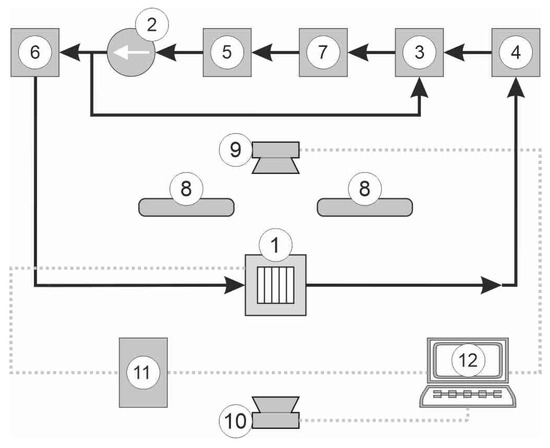
Figure 3. Block diagram of the research stand for the heat transfer investigation during flow boiling in mini-channels: 1—test section, 2—recirculating pump, 3—tank, 4—heat exchanger, 5—filter, 6—Coriolis flow meter, 7—deaerator, 8—LEDs, 9—infrared camera, 10—high-speed camera, 11—data acquisition stations, and 12—PC computer with software.

Figure 3. Block diagram of the research stand for the heat transfer investigation during flow boiling in mini-channels: 1—test section, 2—recirculating pump, 3—tank, 4—heat exchanger, 5—filter, 6—Coriolis flow meter, 7—deaerator, 8—LEDs, 9—infrared camera, 10—high-speed camera, 11—data acquisition stations, and 12—PC computer with software.

Figure 4. Schemes of the test section with mini-channels showing the (a) longitudinal section, (b) top view, and (c) main components; 1—PTFE spacer with mini-channels, 2—PTFE spacer, 3—glass, 4—heated foil, 5—body, 6—top cover, and 7—inlet/outlet chamber with thermocouples K-type ($\mathrm{T}{\mathrm{C}}_{\mathrm{K}1}$, $\mathrm{T}{\mathrm{C}}_{\mathrm{K}2}$).

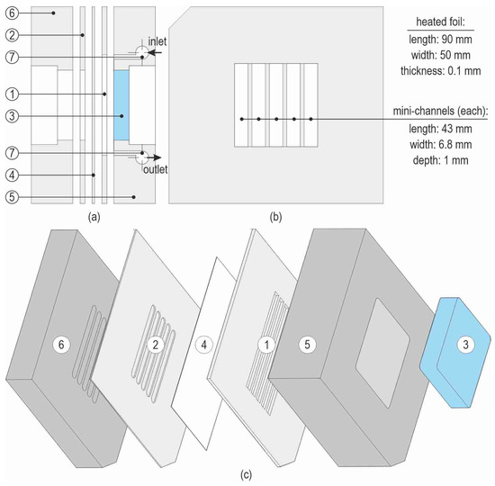
Figure 4. Schemes of the test section with mini-channels showing the (a) longitudinal section, (b) top view, and (c) main components; 1—PTFE spacer with mini-channels, 2—PTFE spacer, 3—glass, 4—heated foil, 5—body, 6—top cover, and 7—inlet/outlet chamber with thermocouples K-type ($\mathrm{T}{\mathrm{C}}_{\mathrm{K}1}$, $\mathrm{T}{\mathrm{C}}_{\mathrm{K}2}$).

In the construction of the test section, a set of parallel rectangular mini-channels was designed. The test section was designed as interchangeable components, allowing for the modification of certain geometric parameters of the mini-channels, such as width, depth, and the number of mini-channels.

The surfaces of each individual mini-channel were created by using the following:

• A heated wall, consisting of a 0.1 mm thick heated foil made of Haynes-230 alloy (‘4’, Figure 4a,c); the heated foil is stretched between metal elements (‘5’ and ‘6’);
• A 6 mm thick glass plate placed in the top cover (‘3’, Figure 4a,c) allows for the observation of two-phase flow structures during fluid flow in the mini-channels;
• The lateral surfaces of the channels with a depth of 1 mm, formed by the PTFE spacer (‘1’, Figure 4a,c).

Electrical insulation between the heated wall and the top cover is ensured by a PTFE-made spacer with a thickness of 0.2 mm (‘2’, Figure 4a,c). The primary metal components of the test section, namely, the body ‘5’ and the top cover ‘6’ (with dimensions of 90 mm × 90 mm × 19 mm), were fabricated from PA-6 using milling technology.

The temperature and pressure of the fluid were measured in the inlet and outlet chambers. K-type thermocouples were used to monitor fluid temperature and are labelled $\mathrm{T}{\mathrm{C}}_{\mathrm{K}1}$ and $\mathrm{T}{\mathrm{C}}_{\mathrm{K}2}$ in the subsequent sections of this article.

4.2. Experimental Procedure

After degassing and stabilising the experimental conditions, the subcooled liquid flows laminarly into an asymmetrically heated mini-channel. When the flow rate and pressure are fixed, there is a gradual increase in the electric power supplied to the foil, followed by an increase in the heat flux transferred to the fluid in the mini-channel:

• Initially, as the heat flux increases, heat transfer between the heated wall and the liquid occurs through single-phase forced convection;
• In the subsequent part of the experiment, the increase in heat flux leads to boiling incipience in the mini-channel, initiating subcooled boiling (subcooled boiling region);
• As the heat flux continues to increase, developed nucleate boiling progresses (saturated boiling region).

4.3. Main Experimental Parameters

Four fluids manufactured by 3M were used as the working fluid in the experimental circulation loop. Specifically, these fluids were HFE-649 (3M Center, St. Paul, MN, USA) (Novec-649, 3M™ Novec™ [36]), HFE-7000 (3M Center, St. Paul, MN, USA) (3M™ Novec™ 7000 Engineered Fluid [37]), HFE-7100 (3M Center, St. Paul, MN, USA) (3M™ Novec™ 7100 Engineered Fluid [38]), and HFE-7200 (3M Center, St. Paul, MN, USA) (3M™ Novec™ 7200 Engineered Fluid [39]).

Table 10. The main properties of the working fluids (according to the data sheets; manufacturer: 3M).

Fluid (HFE-)	Boiling Point Temperature, $\mathbf{K}/°$C	Density (Liquid), kg/m3	Kinematic Viscosity (Liquid), m2/s	Specific Heat (Liquid), J/kg	Thermal Conductivity (Liquid), W/(m·K)	Heat of Evaporation, J/kg
649 [36]	322/49	1600	0.40 × 103	88 × 103	88 × 103	0.069
7000 [37]	307/34	1400	0.32 × 103	142 × 103	142 × 103	0.075
7100 [38]	334/61	1510	0.38 × 103	112 × 103	112 × 103	0.054
7200 [39]	349/76	1430	0.38 × 103	112 × 103	112 × 103	0.068

provides the main properties of these fluids. These fluids, known as hydrofluoroethers (HFEs), are recognised for their environmental friendliness and low ozone depletion potential (ODP), distinguishing them from fluorocarbons (FCs). In particular, HFEs exhibit considerably lower global warming potential (GWP) compared to FCs. According to the manufacturer [40], FC-72 or FC-770 have a GWP greater than 5000, while HFE fluids have a GWP several times lower. For example, HFE-649, HFE-7000, HFE-7100, and HFE-7200 have GWPs of 1, 530, 320, and 55, respectively. Furthermore, FC fluids have an extended atmospheric lifetime (ALR), while HFE-649, HFE-7000, HFE-7100, and HFE-7200 have ALRs of 0.014, 4.9, 4.1, and 0.77 years, respectively. However, the flow boiling performance of dielectric fluids is sometimes affected by thermophysical properties that are less favourable. For example, the thermal conductivity of HFE-7100 is approximately one-tenth that of water, and its latent heat of vaporisation is around 20 times smaller in comparison with that of water.

The uncertainties of the main experimental parameters, recorded during the experimental series, are shown in Table 9. The maximum errors corresponding to the registered experimental parameters are presented for a specified range of temperature or pressure.

The base experimental data regarding each experimental series that were later used in heat transfer calculations are listed in Table 11. For each series, the heat flux values were shown for the entire experiment and only for two sets, which will be referred to as ‘1’ (lower value, within the subcooled boiling region) and ‘2’ (higher value, corresponding to the saturated boiling region) in the further parts of this article.

The main experimental parameters of the series with four refrigerants used as working fluids are reported in Table 11.

Table 11. Main experimental parameters of the series with four refrigerants used as the working fluid.

Parameter	Values or Range
Mass flow rate	0.00556 kg/s
Inlet pressure	0.12 MPa
HFE-649
Heat flux (selected values)	13.25 kW/m2 (No. 1); 17.45 kW/m2 (No. 2)
Fluid temperature at the inlet	288.05 K (No. 1); 288.45 K (No. 2)
Fluid temperature at the outlet	296.95 K (No. 1); 300.05 K (No. 2)
Heat flux (entire experiment)	3.99 ÷ 46.10 W/m2
HFE-7000
Heat flux (selected values)	25.66 kW/m2 (No. 1); 38.06 kW/m2 (No. 2)
Fluid temperature at the inlet	287.75 K (No. 1); 289.35 K (No. 2)
Fluid temperature at the outlet	295.35 K (No. 1); 301.45 K (No. 2)
Heat flux (entire experiment)	4.41 ÷ 55.19 kW/m2
HFE-7100
Heat flux (selected values)	24.43 kW/m2 (No. 1); 31.49 kW/m2 (No. 2)
Fluid temperature at the inlet	290.05 K (No. 1); 289.85 K (No. 2)
Fluid temperature at the outlet	303.05 K (No. 1); 309.95 K (No. 2)
Heat flux (entire experiment)	4.15 ÷ 47.29 kW/m2
HFE-7200
Heat flux (selected values)	29.79 kW/m2 (No. 1); 37.06 kW/m2 (No. 2)
Fluid temperature at the inlet	290.85 K (No. 1); 292.15 K (No. 2)
Fluid temperature at the outlet	296.95 K (No. 1); 300.05 K (No. 2)
Heat flux (entire experiment)	3.49 ÷ 45.30 kW/m2

Table 11. Main experimental parameters of the series with four refrigerants used as the working fluid.

Parameter	Values or Range
Mass flow rate	0.00556 kg/s
Inlet pressure	0.12 MPa
HFE-649
Heat flux (selected values)	13.25 kW/m2 (No. 1); 17.45 kW/m2 (No. 2)
Fluid temperature at the inlet	288.05 K (No. 1); 288.45 K (No. 2)
Fluid temperature at the outlet	296.95 K (No. 1); 300.05 K (No. 2)
Heat flux (entire experiment)	3.99 ÷ 46.10 W/m2
HFE-7000
Heat flux (selected values)	25.66 kW/m2 (No. 1); 38.06 kW/m2 (No. 2)
Fluid temperature at the inlet	287.75 K (No. 1); 289.35 K (No. 2)
Fluid temperature at the outlet	295.35 K (No. 1); 301.45 K (No. 2)
Heat flux (entire experiment)	4.41 ÷ 55.19 kW/m2
HFE-7100
Heat flux (selected values)	24.43 kW/m2 (No. 1); 31.49 kW/m2 (No. 2)
Fluid temperature at the inlet	290.05 K (No. 1); 289.85 K (No. 2)
Fluid temperature at the outlet	303.05 K (No. 1); 309.95 K (No. 2)
Heat flux (entire experiment)	4.15 ÷ 47.29 kW/m2
HFE-7200
Heat flux (selected values)	29.79 kW/m2 (No. 1); 37.06 kW/m2 (No. 2)
Fluid temperature at the inlet	290.85 K (No. 1); 292.15 K (No. 2)
Fluid temperature at the outlet	296.95 K (No. 1); 300.05 K (No. 2)
Heat flux (entire experiment)	3.49 ÷ 45.30 kW/m2

5. Mathematical Model

The intensity of heat transfer in the mini-channels was estimated based on the val ula [41]:

$${\alpha }_{2D}\left(y\right)=\frac{-{\lambda }_F\frac{\partial T_F\left(d_M,y\right)}{\partial x}}{T_F\left(d_M,y\right)-T_{f,bulk}\left(y\right)} ,$$

(4)

${\lambda }_f$—thermal conductivity of the working fluid; $d_{M }$—depth of the mini-channel; $T_F, T_{f,bulk}$—temperature of the heated foil and fluid in the flow core, respectively.

The heated foil ($T_F)$and fluid ${(T}_f)$temperature were determined from the following differential equations [41]:

$${{\kappa }_f\nabla }^2{T}_f-v_y\left(x\right)\frac{\partial T_f}{\partial y}=0 \mathrm{for} \left(x,y\right)\in {\mathsf{\Omega }}_M,$$

(5)

$${\nabla }^2{T}_F=-\frac{q}{d_F{·\lambda }_F} \mathrm{for} \left(x,y\right)\in {\mathsf{\Omega }}_F,$$

(6)

${\mathsf{\Omega }}_M=\left\{\left(x,y\right)\in R^2: 0\le x\le d_M , 0\le y\le L\right\}$, ${\mathsf{\Omega }}_F=\left\{\left(\mathrm{x},\mathrm{y}\right)\in {\mathrm{R}}^2:d_M\le x\le d_M+d_F,0\le y\le L\right\};$ q—heat flux density; L—length of the mini-channel$; d_{F }$—thickness of the heated foil; ${\kappa }_f$—thermal diffusivity coefficient of the working fluid; ${\lambda }_F$—thermal conductivity of the heated foil; $v_y\left(x\right)$—component of the fluid velocity vector.

The boundary conditions are given in Figure 5.

Similarly to [12], the finite element method with the Trefftz-type basis functions was used for solving the inverse heat transfer problem (no boundary condition on the boundary x = 0) in the mini-channel and to determine the heated foil and temperature of the working fluid. A division into rectangular four-noded elements was made for the domain ${\mathsf{\Omega }}_M\cup {\mathsf{\Omega }}_F$. The temperature in each element was estimated using a linear combination of the Trefftz-type basis functions:

$$T_{f }^j\left(x,y\right)={\sum }_{k=1}^N{\widehat{T}}_f^r\left(x_{jk},y_{jk}\right)f_{jk}\left(x,y\right) \mathrm{i}\mathrm{n} {\mathsf{\Omega }}_{j,M} \mathrm{f}\mathrm{o}\mathrm{r} \mathrm{j}=\mathrm{1,2},\dots ,{\mathrm{J}}_M,$$

(7)

$$\begin{gathered} T_{F }^j\left(x,y\right)=u\left(x,y\right)+\sum _{k=1}^N\left({\widehat{T}}_F^r\left(x_{jk},y_{jk}\right)-u\left(x_{jk},y_{jk}\right)\right)g_{jk}\left(x,y\right) \\ \mathrm{i}\mathrm{n} {\mathsf{\Omega }}_{j,F} \mathrm{f}\mathrm{o}\mathrm{r} \mathrm{j}=\mathrm{1,2},\dots ,{\mathrm{J}}_F, \end{gathered}$$

(8)

${\bigcup }_{j=1}^{{\mathrm{J}}_M}{\mathsf{\Omega }}_{j,M}={\mathsf{\Omega }}_M$, ${\bigcup }_{j=1}^{{\mathrm{J}}_F}{\mathsf{\Omega }}_{j,F}={\mathsf{\Omega }}_F$, $J_M$—the number of elements in ${\mathsf{\Omega }}_M$, $J_F$—the number of elements in ${\mathsf{\Omega }}_F$; $u\left(x,y\right)$—the particular solution to Equation (6), $f_{jk}\left(x,y\right)$—the basis functions exactly satisfying the Fourier–Kirchhoff equation$;{ g}_{jk}\left(x,y\right)$—the basis functions strictly satisfying the Laplace’s equation$; {\widehat{T}}_f^r$—the temperature value in the r-th node of domain ${\mathsf{\Omega }}_M\cup {\mathsf{\Omega }}_F$; ${\widehat{T}}_F^r$—the temperature value in the r-th node of domain${\mathsf{\Omega }}_M\cup {\mathsf{\Omega }}_F$, j—element number; k—basis function number in j-th element; r—node number in the entire domain ${\mathsf{\Omega }}_F\cup {\mathsf{\Omega }}_M$; N—the number of nodes in the element.

By minimising the appropriate function, as in [41], the unknown coefficients ${\widehat{T}}_f^r$ and ${\widehat{T}}_F^r$ were computed. This function indicates the mean square error of the approximation solution on the domain boundaries and at the common edges of adjacent subdomains.

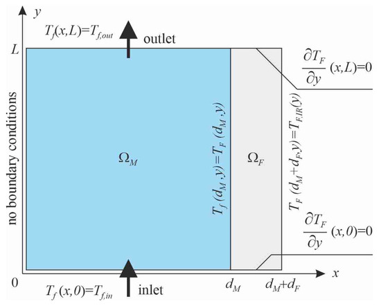
Figure 5. A scheme showing the boundary conditions taken into the 2D mathematical model; $T_{f,in}, T_{f,out}$—the fluid temperature at the inlet and outlet of the mini-channel; $T_{F, IR}$—the temperature of the heated foil measured by an infrared camera.

Figure 5. A scheme showing the boundary conditions taken into the 2D mathematical model; $T_{f,in}, T_{f,out}$—the fluid temperature at the inlet and outlet of the mini-channel; $T_{F, IR}$—the temperature of the heated foil measured by an infrared camera.

In the numerical calculations, performed in the Mathematica program of Wolfram Research ver. 13, the assumed grid density should be verified to ensure the correctness of the results. In the computations, the determination of the local heat transfer coefficients is crucial. In the analyses, fluid bulk temperatures were selected as the base parameter due to their importance in determining the resultant heat transfer coefficient values. The process of choosing the density of the data from the experimental calculation for HFE-649 fluid was demonstrated. Seven grid sizes (n = 70, 80, 90, 100, 110, 120, and 130) were considered in the analyses, with the primary focus on the grid size in relation to the flow direction, specifically the length of the mini-channel. The total numbers of elements in both sub-domains, i.e., the mini-channel (fluid) and heated foil, as well as the total number of nodes, are listed in

Table 12. Main characteristics of grids considered in the calculations (experiment with fluid HFE-649).

n (Grid Size)	70	80	90	100	$110$	120	130
Total number of elements	490	560	630	700	770	840	910
Total number of nodes	569	649	729	809	889	969	1049

for each grid size.

The average relative difference, $\epsilon$, between the h values (considering fluid bulk temperatures, $T_{f,bulk}$, and the heat transfer coefficient, $\alpha$, separately), obtained on the basis of the data collected for the adjacent values of the different grid sizes, n, given in Table 12, is calculated as follows:

$$\epsilon \left(i,j\right)=\sqrt{\frac{1}{m}\sum _{k=1}^m\frac{{\left(h\left(i,k\right)-h(j,k)\right)}^2}{min\left({\left(h\left(i,k\right)\right)}^2,{\left(h(j,k)\right)}^2\right)}, } h=T_{f,bulk},\alpha ,$$

(9)

where m denotes the number of temperature measurements obtained by the IR camera.

The results of the procedure for the relative differences of fluid bulk temperature and heat transfer coefficient determination are shown in

Table 13. Average relative differences between fluid bulk temperatures and heat transfer coefficients for adjacent values of grid size n.

Heat Flux Value/No.	$\mathit{\epsilon }\left(\mathbf{70}\mathbf{,}\mathbf{80}\right)$ ${\mathbf{10}}^{\mathbf{-}\mathbf{3}}$	$\mathit{\epsilon }\left(\mathbf{80}\mathbf{,}\mathbf{90}\right)$ ${\mathbf{10}}^{\mathbf{-}\mathbf{3}}$	$\mathit{\epsilon }\left(\mathbf{90}\mathbf{,}\mathbf{100}\right)$ ${\mathbf{10}}^{\mathbf{-}\mathbf{3}}$	$\mathit{\epsilon }\left(\mathbf{100}\mathbf{,}\mathbf{110}\right)$ ${\mathbf{10}}^{\mathbf{-}\mathbf{3}}$	$\mathit{\epsilon }\left(\mathbf{110}\mathbf{,}\mathbf{120}\right)$ ${\mathbf{10}}^{\mathbf{-}\mathbf{3}}$	$\mathit{\epsilon }\left(\mathbf{120}\mathbf{,}\mathbf{130}\right)$ ${\mathbf{10}}^{\mathbf{-}\mathbf{3}}$
differences between fluid bulk temperatures
13.25 [kW/m2]/No. 1	0.3	0.2	0.2	0.1	0.1	0.1
17.45 [kW/m2]/No. 2	0.3	0.3	0.2	0.1	0.1	0.1
differences between heat transfer coefficients
13.25 [kW/m2]/No. 1	0.8	0.6	0.5	0.4	0.4	0.3
17.45 [kW/m2]/No. 2	0.5	0.4	0.3	0.3	0.2	0.2

. Calculations were made for the two adjacent values of grid size n (see Table 12). Six variants were considered: $\epsilon$(70,80) (for n = 70 and n = 80), $\epsilon$(80,90) (for n = 80 and n = 90), …, and $\epsilon$(120,130) (for n = 120 and n = 130). Each of the cases was determined on the basis collected for the two values of heat flux (No. 1—13.25 kW/m² and No. 2—17.45 kW/m²).

The maximum values of the average relative differences, $\epsilon$, considering fluid bulk temperature and heat transfer coefficients, were observed for the smallest values on n, specifically for (70 and 80), i.e., for $\epsilon \left(\mathrm{70,80}\right)$. The relative differences were diminished, achieving a low, constant value in the following:

• Fluid bulk temperature analysis for ε(100,110) = 0.1 $\times {10}^{-3}$ (both values of heat flux);
• Heat transfer coefficient analysis for ε(100,110) = 0.4 $\times {10}^{-3}$ (lower value for heat flux) and ε(110,120) = 0.2 $\times {10}^{-3}$ (higher value for heat flux).

In the calculations of the relative differences, the fluid temperature is directly determined. Therefore, these results heavily influence the selection of the grid parameter value, n, in comparison to the case of the relative differences in the heat transfer coefficient. Based on this consideration, n = 100 was assumed to be sufficiently accurate. Finally, the size of the base grid selected for further calculations was n = 100, resulting in 700 elements and 807 nodes.

6. Results of Heat Transfer Experiment

6.1. General Characteristics of Heat Transfer Processes

In the experimental conditions, a subcooled liquid (in laminar flow) enters the asymmetrically heated mini-channel. Initially, with an increase in heat flux density, the heat transfer between the heated foil and the liquid takes place through forced single-phase convection. In the near-wall layer adjacent to the foil, the liquid undergoes superheating, whereas in the core of the flow and near the quasi-adiabatic surface (glass plate), it remains subcooled. This results in a significant temperature gradient over a small depth of the mini-channel. Increasing the heat flux supplied to the heated foil activates the vapour nuclei on the heater surface. The abrupt decrease in the temperature of the heated wall surface is caused by bubbles spontaneously forming in the near-wall layer. A further increase in the heat flux causes subcooled boiling to transform into saturated (developed) boiling, and the heated foil surface becomes superheated. Vapour bubbles expand and combine into larger agglomerates near the mini-channel outlet.

6.2. General Characteristics of the Results

Four refrigerants (HFE-649, HFE-7000, HFE-7100, and HFE-7200) were applied as the working fluid flowing along five mini-channels of the horizontal test section. The flow direction was above the heated wall, indicating that the test section was subjected to asymmetric heating. The heated wall temperature of the mini-channels was measured using infrared thermography. The distribution of the working fluid temperature in the central mini-channel, determined through infrared measurements and mathematical calculations, was presented for each working fluid (HFE-649, HFE-7000, HFE-7100, and HFE-7200), as they depend on the following:

• Bulk temperature (calculated on the basis of the assumed linear dependence between the measurements at the inlet and the outlet), Figure 6a,c,e,g;
• Temperature on the fluid contact surface with the heated foil, Figure 6b,d,f,h, with both as a function of the distance from the mini-channel inlet.

The local heat transfer coefficients between the heated foil and the refrigerant flowing in the mini-channel were calculated from the Robin condition with the aid of the FEM with the Trefftz functions. The dependencies of the heat transfer coefficient as a function of the distance from the mini-channel inlet are shown in Figure 7 (separately for each working fluid). Furthermore, heat transfer coefficient vs. distance from the inlet, obtained from the calculations using the 2D mathematical method and Newton’s law of cooling are illustrated in Figure 8.

Example boiling curves, which illustrate the dependence of heat flux as a function of the temperature difference (defined as the temperature of the heated wall minus the temperature of the fluid bulk), are shown in Figure 9.

Furthermore, example two-phase flow patterns are presented in Figure 10 as captured images and binarized versions.

Several observations and conclusions concerning the collected data and results are shown and discussed in the later part of this chapter.

6.3. Temperature Data and Analyses

The temperatures of the working fluid and the heated wall were collected for four working fluids: HFE-649, HFE-7000, HFE-7100, and HFE-7200. The data were obtained for two selected values of heat flux, one representing the subcooled boiling region and the other the saturated boiling region, as functions of the distance from the inlet. The results are illustrated as temperature vs. distance from the mini-channel inlet for each of the fluids, additionally, i.e., Figure 6a,b (HFE-649), Figure 6c,d (HFE-7000), Figure 6e,f (HFE-7100), and Figure 6g,h (HFE-7200), where the graphs concern fluid bulk temperature (part a) or, in the other case, the graphs regard temperature at contact with the heated foil (part b).

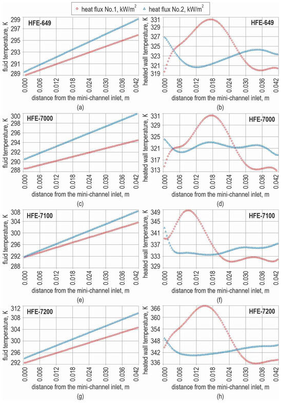
Figure 6. Temperature of the working fluid vs. distance from the mini-channel inlet, obtained from calculations performed for two values of heat flux: (a,c,e,g) bulk temperature (calculated on the basis of the assumed linear dependence between the measurements at the inlet and the outlet); (b,d,f,h) temperature at the contact surface with the heated foil; the results for the working fluids: (a,b) HFE-649; (c,d) HFE-7000; (e,f) HFE-7100; (g,h) HFE-7200.

Figure 6. Temperature of the working fluid vs. distance from the mini-channel inlet, obtained from calculations performed for two values of heat flux: (a,c,e,g) bulk temperature (calculated on the basis of the assumed linear dependence between the measurements at the inlet and the outlet); (b,d,f,h) temperature at the contact surface with the heated foil; the results for the working fluids: (a,b) HFE-649; (c,d) HFE-7000; (e,f) HFE-7100; (g,h) HFE-7200.

All four cooling fluids differ slightly in their physical properties, especially regarding boiling point. The bulk temperature of the working fluid in the fluid core monotonically increases with the distance from the inlet (Figure 6a,c,e,g). The highest temperature was recorded for HFE-7200. The values directly resulted from the assumption of a linear dependence between the inlet and outlet in the local fluid calculation.

By considering the temperature at the fluid contact surface with the heated foil, the subsequent findings can be summarised as follows:

○

Results for heat flux No. 1 (lower value):

• Temperature dependence from the inlet to two-thirds of the length initially increases and then decreases;
• The maximum temperature corresponds to the initiation of boiling;
• Spontaneous nucleation causes a drop in the temperature of the heated foil surface, termed ‘nucleation hysteresis,’ absorbing a significant amount of energy transferred to the liquid;
• Near the outlet, the values do not change significantly anymore.

○

Results for heat flux No. 2 (higher value):

• Throughout the entire length, the temperature dependence exhibits a polynomial character without strong extremes;
• In the outlet section, temperatures reach higher values compared to those obtained for a lower heat flux.

During the comparative analysis, a similar temperature distribution was observed at the fluid-heater interface, but the temperature values were higher for the HFE-7100 fluid and the highest for HFE-7200. As indicated above, the tested fluids are characterised by various boiling point values (the highest are for HFE-7100 and HFE-7200 in comparison to other fluids, i.e., HFE-649 and HFE-7000).

6.4. Heat Transfer Coefficient Results

The dependencies of the heat transfer coefficient (HTC) as a function of distance from the inlet are illustrated in Figure 7 (separately for each working fluid). The dependencies were based on the results of the calculations performed for two values of heat flux, similar to the dependencies of the fluid temperatures, as shown in Figure 6.

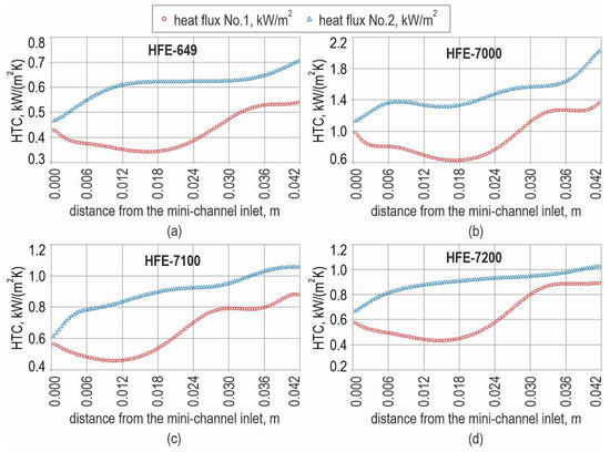
Figure 7. Heat transfer coefficient vs. distance from the mini-channel inlet, obtained from calculations performed for two values of heat flux and the working fluid: (a) HFE-649; (b) HFE-7000; (c) HFE-7100; (d) HFE-7200.

Figure 7. Heat transfer coefficient vs. distance from the mini-channel inlet, obtained from calculations performed for two values of heat flux and the working fluid: (a) HFE-649; (b) HFE-7000; (c) HFE-7100; (d) HFE-7200.

An analysis of the data in Figure 7 reveals that higher heat transfer coefficients are obtained for increased heat flux. The distribution of HTC results is similar for all the fluids tested. Generally, an observed increase in HTC values was observed with a slight increase in the distance from the mini-channel inlet, particularly pronounced in the case of HFE-7000. The highest HTC values were noted for fluid HFE-7000 (Figure 7b), reaching 2.1 [kW/(m² K)] at higher heat flux, while the lowest was observed for fluid HFE-649 (Figure 7a), approximately 0.35 [kW/(m² K)] at lower heat flux. Comparable HTC values were gained for the HFE-7100 and HFE-7200 fluids at a higher heat flux, up to 1.05 [kW/(m² K)] (Figure 7c,d). The HTC values obtained for the higher heat flux for all fluids tested exhibited more significant differences compared to those collected at a lower heat flux. Furthermore, similar HTC values were observed for three other working fluids (HFE-649, HFE-7100, and HFE-7200), considering the results achieved with lower heat flux. It should be emphasised that the experiment using HFE-7000 as the working fluid achieved the highest heat transfer coefficients compared to the other fluids tested, confirming the previous results [42].

6.5. Validation of the Heat Transfer Results

The heat transfer coefficient, derived from the Robin condition and determined using the finite element method (FEM) with Trefftz functions based on the proposed 2D mathematical model, was validated using a simpler method. In this alternative approach, the heat transfer coefficients were determined by using Newton’s law of cooling. The calculation involved the temperature of the heated wall (measured from the outer surface) and the local fluid bulk temperature to calculate the temperature difference as follows:

$${\alpha }_{1D}\left(y_i\right)=\frac{q}{T_{F,IR}\left(y_i\right)-(T_{f,in}+\frac{T_{f,out}-T_{f,in}}{L}{y}_i)} ,$$

(10)

where $q, T_{F,IR}, T_{f,in}$, $T_{f,out}, L$ have the same meaning as in Equations (5) and (6) and in the boundary conditions presented in Figure 5.

The average relative differences between the heat transfer coefficients obtained by means of the FEM with Trefftz functions and those based on Newton’s law of cooling are determined using the following formula:

$${rd}_k=\sqrt{\frac{1}{m}\sum _{i=1}^m\frac{{\left({\alpha }_{1D}\left(y_i\right)-{\alpha }_{2D}\left(y_i\right)\right)}^2}{{\left({\alpha }_{1D}\left(y_i\right)\right)}^2}, }k=\mathrm{H}\mathrm{F}\mathrm{E}-649,\mathrm{H}\mathrm{F}\mathrm{E}-7000,\mathrm{H}\mathrm{F}\mathrm{E}-7100,\mathrm{H}\mathrm{F}\mathrm{E}-7200,$$

(11)

where ${\alpha }_{1D}$ and ${\alpha }_{2D}$ are defined by Equation (4) and Equation (10), respectively.

The average relative differences, ${rd}_k$, between the heat transfer coefficients obtained from the 2D mathematical model (using the FEM with Trefftz functions) and Newton’s law of cooling are presented in

Table 14. Average relative differences between heat transfer coefficients due to 2D mathematical modelling and Newton’s law of cooling.

Heat Flux	${\mathit{r}\mathit{d}}_{\mathit{H}\mathit{F}\mathit{E}\mathbf{-}\mathbf{649}}$ %	${\mathit{r}\mathit{d}}_{\mathit{H}\mathit{F}\mathit{E}\mathbf{-}\mathbf{7000}}$ %	${\mathit{r}\mathit{d}}_{\mathit{H}\mathit{F}\mathit{E}\mathbf{-}\mathbf{7100}}$ %	${\mathit{r}\mathit{d}}_{\mathit{H}\mathit{F}\mathit{E}\mathbf{-}\mathbf{7200}}$ %
No.1	0.6	3.7	1.6	0.4
No.2	0.8	1	1	0.6

.

When analysing the results presented in Table 14, it becomes evident that the results of both calculations (using the 2D method with the FEM and Trefftz functions and those based on Newton’s law of cooling) yielded very similar values. The average relative differences fell within the range of 0.6–3.7%, with the highest occurring in the experiment with HFE-7000 and lower heat flux (No. 1) reaching 3.7%.

Figure 8 illustrates the selected results from the calculations using the 2D method and Newton’s law of cooling to visualise the data distribution for comparison. The data for the calculations were obtained from experiments with HFE-649 and are presented for the two values of heat flux.

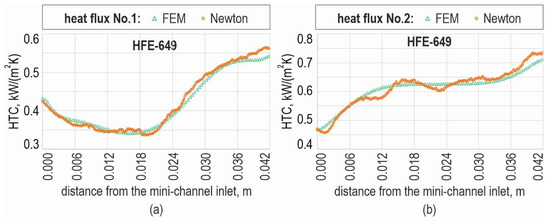
Figure 8. Heat transfer coefficient vs. distance from the mini-channel inlet, obtained from the calculations using the 2D mathematical method (named ‘FEM’) and Newton’s law of cooling (named ‘Newton’) for an experiment on HFE-649; the results obtained for the two values of heat flux: (a) 13.25 kW/m² (No. 1) and (b) 17.45 kW/m² (No. 2).

Figure 8. Heat transfer coefficient vs. distance from the mini-channel inlet, obtained from the calculations using the 2D mathematical method (named ‘FEM’) and Newton’s law of cooling (named ‘Newton’) for an experiment on HFE-649; the results obtained for the two values of heat flux: (a) 13.25 kW/m² (No. 1) and (b) 17.45 kW/m² (No. 2).

6.6. Boiling Curves

The efficiency of the boiling process is commonly assessed through the behaviour of the boiling curve, which establishes the dependence of the heat flux density on the wall superheat. The slope of the boiling curve rises as the heat flux increases, indicating that an escalating number of nucleation sites become active with higher superheat as long as the system is far from the boiling crisis (critical heat flux). However, the decrease in superheat as boiling starts is attributed to a change in nucleation dynamics regarding the formation of the first bubbles and their detaching from the heated surface. Spontaneous nucleation causes a drop in the temperature of the heater surface, called ‘nucleation hysteresis’.

In this work, the data from the experiments have not covered critical heat flux occurrence, but they cover single-phase convection, the onset of boiling, the subcooled boiling region, and the developed (saturated) boiling region.

The boiling curves were constructed as heat flux density vs. temperature difference (temperature of the heated wall to the temperature of the fluid bulk). The boiling curves depicted in Figure 9 were created for three points in the central mini-channel, with respect to the selected distances from the inlet: approximately one-third, one-half, and two-thirds of the mini-channel length. The curves were constructed for four tested cooling liquids separately, i.e., for HFE-649 (Figure 9a), HFE-7000 (Figure 9b), HFE-7100 (Figure 9c), and HFE-7200 (Figure 9d).

Each of the boiling curves exhibits the typical course of the function and distribution of the data with the occurrence of nucleation hysteresis when the boiling process starts. The analysis was carried out on the typical boiling curves, illustrated for HFE-649 in Figure 9a. As the subcooled liquid flows into a mini-channel (represented by the bottom line of the graph up to a point named ONB), an increase in the heat flux leads to the onset of nucleate boiling. In the area adjacent to the plate, the fluid was superheated, but in the flow core, it was subcooled. Spontaneous nucleation causes a drop in the temperature of the heated plate surface, and “nucleation hysteresis” occurs. Bubbles, which absorb a significant amount of energy transferred to the liquid, act as internal heat sinks. The results confirm the previous findings of the authors, published, among others, in [41,42,43]. When subcooled boiling gradually transforms into developed nucleate boiling (where the liquid reaches the saturation temperature), there is also an increase (sometimes a very slight increase) in this part of the boiling curve. The increase in the heat flux causes an increase in the vapour phase content in the two-phase mixture, which leads to an increase in the pressure value and its fluctuations. When analysing the boiling curves presented in Figure 9, it is evident that, for all dependencies, the most significant temperature difference drops characteristic of nucleation hysteresis were observed for HFE-7200 (Figure 9d), with a temperature difference of about 35 K. The onset of boiling occurred at the lowest value of heat flux compared to all tested fluids. The temperature difference at ONB was the lowest for HFE-649 (Figure 9a), with a difference value of approximately 15 K. For HFE-7000 (Figure 9b) and HFE-7100 (Figure 9c), the temperature difference was approximately 25 K. Upon further analysis of the boiling curve dependencies, it was observed that the temperature differences corresponding to boiling incipience noted for higher heat flux values are observed for two fluids (HFE-7000 and HFE-7200), while for the lowest heat flux, it was observed for HFE-649. When analysing the sections regarding developed nucleate boiling, it was observed that the HFE-7100 curves are almost parallel. Furthermore, in the vicinity of ONB, a large scatter of points is observed on the graph. The superheat of the heated wall surface corresponding to ONB decreases with increasing distance from the mini-channel inlet. The relationship for all fluids in the section regarding the saturated boiling region in the boiling curve courses, considering three distances (one-third, one-half, and two-thirds of the mini-channel length), is shifted in the graph by a temperature difference value of about 5 K.

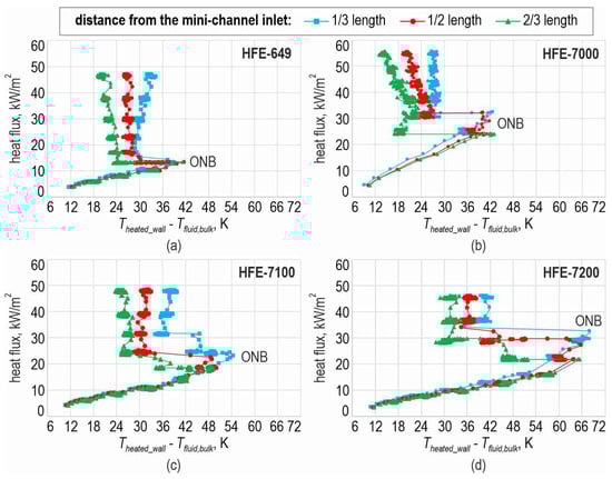
Figure 9. Boiling curves, constructed at three selected distances from the mini-channel inlet: one-third, one-half, and two-thirds the mini-channel length; results obtained for (a) HFE-649; (b) HFE-7000; (c) HFE-7100; (d) HFE-7200; ONB—onset of nucleate boiling.

Figure 9. Boiling curves, constructed at three selected distances from the mini-channel inlet: one-third, one-half, and two-thirds the mini-channel length; results obtained for (a) HFE-649; (b) HFE-7000; (c) HFE-7100; (d) HFE-7200; ONB—onset of nucleate boiling.

6.7. Two-Phase Flow Patterns

In Figure 10, examples of two-phase flow patterns which were captured during the experiment with HFE-7000 as the working fluid are shown. The selected images correspond to the lowest (part a) and highest (part d) heat flux values. In Figure 10a–d, the data pertain to the recorded images, while Figure 10e–h depict these images in a binarised form.

In the flow patterns images, small spherical vapour bubbles are observed. The region where the onset of boiling begins is precisely delineated. The bubbles are fragmented and fairly evenly distributed in the boiling region, from the onset of nucleate boiling to the outlet of the mini-channels. In Figure 10a,b,e,f, the boiling front, accompanying the boiling incipience, is indicated by red lines.

Figure 10. Images of flow patterns captured during the experiment with HFE-7000 as the working fluid; images (a–d) depict the recorded flow patterns, while images (e–h) show the binarised versions; heat flux values: (a) 25.66 kW/m², (b) 30.54 kW/m², (c) 34.63 kW/m², and (d) 38.06 kW/m²; the boiling front position is marked by a red line.

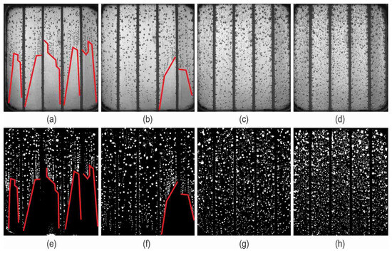
Figure 10. Images of flow patterns captured during the experiment with HFE-7000 as the working fluid; images (a–d) depict the recorded flow patterns, while images (e–h) show the binarised versions; heat flux values: (a) 25.66 kW/m², (b) 30.54 kW/m², (c) 34.63 kW/m², and (d) 38.06 kW/m²; the boiling front position is marked by a red line.

Based on our own previous research [42,43], two types of two-phase flow structures were recognised in the flow pattern: bubbly and bubbly-slug. Tiny spherical vapour bubbles are visible during the forming process as boiling starts and continues to develop, which is characteristic of bubbly flow. Additionally, it can be stated that the occurrence of a bubbly-slug pattern has begun, wherein small bubbles aggregate into larger, uneven ones (see Figure 10c,d). Slug, wispy annular, asymmetrical wispy annular, and mist structures were not observed in the captured two-phase flow images. It is worth noting that the previous investigations focused on research involving a single mini-channel that was significantly longer than the mini-channel currently tested here. Furthermore, the analysis also included the observation of flow structures for channels with various spatial orientations. In this study, the channel was positioned horizontally with the fluid flow over the heated wall.

7. Conclusions

This article aims to experimentally investigate boiling heat transfer during cooling fluid flow in rectangular mini-channels. In the experimental sets, four working fluids were applied (HFE-649, HFE-7000, HFE-7100, and HFE-7200). Furthermore, the proposal of a 2D mathematical model for heat transfer helped to determine the heat transfer coefficient from the Robin condition and FEM with Trefftz functions was used to solve the inverse heat transfer problem.

In the experimental series, K-type thermocouples and infrared thermography were employed for measuring temperature. In terms of precious temperature measurements, the study also includes detailed uncertainty analyses for temperature measurements from K- and T-type thermocouples. The uncertainty analyses involved estimating the uncertainties in the temperature measurements obtained from both K- and T-type thermocouples. The experiments were carried out using a temperature calibrator, a high-precision RTD sensor, and a specialised thermometer serving as a data acquisition station. The results of the uncertainty estimation for temperature measurements were presented in detail and thoroughly analysed. The calculations were performed using two statistical methods: the uncertainty propagation method and the Monte Carlo method. Finally, the expanded uncertainties were calculated according to both calculation methods, and these were compared. The ultimate uncertainty was related to the measurement paths. The expanded uncertainties for the T-type thermocouple did not exceed 0.89 °C, and for the K-type, they achieved 2.47 °C. The results obtained from both methods yielded similar outcomes.

The results of the flow boiling heat transfer experiments included analyses of temperature, heat transfer coefficients, the boiling curve course, and flow pattern images. The most important findings based on the research and analysis of the results are enumerated below.

A similar temperature distribution at the fluid-heater interface was observed, but the temperature values differ, especially for the two fluids. Furthermore, when analysing the temperature results, the following observations were made:

• Lower values of the working fluid temperature were observed when two fluids were examined (HFE-649 and HFE-7000);
• The highest temperature was observed for HFE-7200 compared to other tested fluids;
• The highest temperature in contact with the heated foil was achieved when HFE-7200 was used as the working fluid in the experiment with a higher heat flux value;
• By taking into account the temperature of the working fluid, it was observed that it monotonically increased from the inlet to the outlet;
• Higher temperature values at the contact between the working fluid and the heated foil surface were noticed in the first half of the distance (from the inlet).

The main observations regarding the heat transfer coefficient (HTC) results are as follows:

• The highest HTC values, compared to other tested fluids, were achieved in experiments using HFE-7000 as the working fluid (considering a higher heat flux value);
• The lowest HTC was observed for HFE-649 compared to all tested fluids;
• Similar values were achieved for two working fluids (HFE-7100 and HFE-7200);
• Generally, an increase in HTC values was observed, with a slight increase in the distance from the mini-channel inlet, particularly noticeable for HFE-7000.

The essential findings from the analysis of boiling curve courses can be emphasised:

• The boiling curves exhibit the typical shape of the ‘nucleation hysteresis’ phenomenon;
• Based on the boiling curve courses, the highest temperature differences corresponding to boiling incipience were obtained for the HFE-7200 fluid, and the lowest temperature differences were achieved for HFE-649.

Upon analysis of the two-phase flow patterns, it was observed that only small spherical vapour bubbles were identified at the onset of the boiling process, indicating a bubbly pattern. As the boiling process progressed, the images also revealed the presence of a bubbly-slug pattern.

It seems that flow boiling heat transfer has the potential to significantly enhance efficiency and reduce the cost of cooling systems. Although flow boiling is crucial for cooling miniature devices, such as high-power electronic devices in microelectronics, comprehensive studies have been limited, mainly due to the complex nature of the phase-change process. In addition to the demand for efficient cooling and miniaturisation, there is a growing interest in the use of environmentally friendly cooling fluids, particularly dielectric coolants.

Among the various cooling techniques, flow boiling in mini-channels stands out as one of the most effective and efficient approaches for future thermal management. Extensive studies have been conducted to enhance flow boiling in mini-channels by promoting nucleation through physical surface modifications. Novel surface microstructures for flow boiling, including hydrophilic, hydrophobic, and biophilic surfaces, will be utilised in expanded experimental studies.

Future research will also explore the impact of nanofluids, employing heating surfaces with different physical properties in terms of roughness and resulting surface wettability. The examination of modified heated surfaces and cooling fluids with nanoparticles aims to achieve the highest possible heat transfer coefficients.

In conclusion, it is important to emphasise the lack of identified solutions for determining uncertainties in contact temperature measurements in the existing literature, especially based on specialist experimental investigations. However, achieving the highest accuracy of measurements requires procedures that comply with standards. The authors of this work have made an attempt to address this gap.

References

- Hieu, H.N.; Agustiarini, N.; Oh, J.T. Flow Boiling Heat Transfer Coefficient and Pressure Drop of R448A inside Various Multiport Tubes: An Experimental Investigation and Correlation Assessment. Int. J. Heat Mass Transf. 2023, 217, 124610. [Google Scholar] [CrossRef]
- Lillo, G.; Mastrullo, R.; Mauro, A.W.; Pelella, F.; Viscito, L. Experimental Thermal and Hydraulic Characterization of R448A and Comparison with R404A during Flow Boiling. Appl. Therm. Eng. 2019, 161, 114146. [Google Scholar] [CrossRef]
- Lioger-Arago, R.; Coste, P.; Caney, N. Study of Flow Boiling in a Vertical Mini-Channel with Surface Structuring: Heat Transfer Analysis Using Inverse Method. Int. J. Therm. Sci. 2023, 192, 108392. [Google Scholar] [CrossRef]
- Li, G.; Zhuang, D.; Xie, L.; Ding, G.; Yue, B.; Fan, B.; Zhang, H.; Shao, Y. Development of Boiling Flow Pattern Map and Heat Transfer Correlation of R32-Oil Mixture inside a Horizontal Micro-Fin Tube. Int. J. Refrig. 2023, 155, 320–332. [Google Scholar] [CrossRef]
- Luo, X.; Xia, Y.; Huang, J.; He, J.; Tu, J.; Chen, J.; Liang, Y.; Yang, Z.; Chen, Y. Experimental Investigation on High-Temperature Flow Boiling Heat Transfer Characteristics of R245fa in a Horizontal Circular Tube. Appl. Therm. Eng. 2023, 225, 120260. [Google Scholar] [CrossRef]
- Haag, M.; Selvam, P.K.; Leyer, S. Effect of Condenser Tube Inclination on the Flow Dynamics and Instabilities in a Passive Containment Cooling System (PCCS) for Nuclear Safety. Nucl. Eng. Des. 2020, 367, 110780. [Google Scholar] [CrossRef]
- Straubinger, D.; Illés, B.; Busek, D.; Codreanu, N.; Géczy, A. Modelling of Thermocouple Geometry Variations for Improved Heat Transfer Monitoring in Smart Electronic Manufacturing Environment. Case Stud. Therm. Eng. 2022, 33, 102001. [Google Scholar] [CrossRef]
- Hetsroni, G.; Gurevich, M.; Mosyak, A.; Rozenblit, R. Surface Temperature Measurement of a Heated Capillary Tube by Means of an Infrared Technique. Meas. Sci. Technol. 2003, 14, 807–814. [Google Scholar] [CrossRef]
- Kumavat, P.S.; Alimohammadi, S.; O’Shaughnessy, S.M. An Experimental-Numerical Study of Heat Transfer Enhancement in a Minichannel Using Asymmetric Pulsating Flows. IEEE Trans. Compon. Packag. Manuf. Technol. 2023, 13, 1147–1154. [Google Scholar] [CrossRef]
- Wang, C.S.; Wang, E.S.; Huang, Y.J.; Liou, T.M. PIV and IRT Measurements of Hydrothermal Performance in a U-Shaped Heat Exchanger with 3D Printed Detached Curved Ribs. Int. J. Heat Mass Transf. 2023, 201, 123562. [Google Scholar] [CrossRef]
- Hożejowska, S.; Kaniowski, R.M.; Poniewski, M.E. Experimental Investigations and Numerical Modeling of 2D Temperature Fields in Flow Boiling in Minichannels. Exp. Therm. Fluid Sci. 2016, 78, 18–29. [Google Scholar] [CrossRef]
- Maciejewska, B. The Application of Beck’s Method Combined with FEM and Trefftz Functions to Determine the Heat Transfer Coefficient in a Minichannel. J. Theor. Appl. Mech. 2017, 55, 103–116. [Google Scholar] [CrossRef]
- JCGM 101:2008 Evaluation of Measurement Data—Supplement 1 to the “Guide to the Expression of Uncertainty in Measurement”—Propagation of Distributions Using a Monte Carlo Method; Joint Committee for Guides in Metrology (JCGM). Int. Organ. Stand. Geneva ISBN 2008, 50, 134.
- Pearce, J.V.; Harris, P.M.; Greenwood, J.C. Evaluating Uncertainties in Interpolations between Calibration Data for Thermocouples. Int. J. Thermophys. 2010, 31, 1517–1526. [Google Scholar] [CrossRef]
- JCGM 100: 2008 Evaluation of Measurement Data—Guide to the Expression of Uncertainty in Measurement. Jt. Comm. Guides Metrol. (JCGM) 2008, 1, 1–120.
- Ferreira-Oliveira, J.R.; de Lucena, L.R.R.; dos Reis, R.P.B.; de Araújo, C.J.; Bezerra-Filho, C.R.; Arencibia, R.V. Uncertainty Quantification Through Use of the Monte Carlo Method in a One-Dimensional Heat Conduction Experiment. Int. J. Thermophys. 2020, 41, 1–19. [Google Scholar] [CrossRef]
- Ferreira-Oliveira, J.R.; dos Santos-Junior, J.A.; Medeiros, V.S.; Guimarães, G. Thermal Conductivity Measurement of a Polymer Material Using a Steady-State Temperature Field. Exp. Technol. 2023, 47, 483–491. [Google Scholar] [CrossRef]
- Forster, M.; Seibold, F.; Krille, T.; Waidmann, C.; Weigand, B.; Poser, R. A Monte Carlo Approach to Evaluate the Local Measurement Uncertainty in Transient Heat Transfer Experiments Using Liquid Crystal Thermography. Meas. J. Int. Meas. Confed. 2022, 190, 110648. [Google Scholar] [CrossRef]
- Díaz-Pérez, L.C.; Torralba, M.; Muro, L.; Albajez, J.A.; Yagüe-Fabra, J.A. Uncertainty Budget of a Large-Range Nanopositioning Platform Based on Monte Carlo Simulation. Meas. J. Int. Meas. Confed. 2023, 208, 112469. [Google Scholar] [CrossRef]
- Brown, R.J.C.; Brown, A.S.; Yardley, R.E.; Corns, W.T.; Stockwell, P.B. A Practical Uncertainty Budget for Ambient Mercury Vapour Measurement. Atmos. Environ. 2008, 42, 2504–2517. [Google Scholar] [CrossRef]
- Vlaeyen, M.; Haitjema, H.; Dewulf, W. Virtual Task-Specific Measurement Uncertainty Determination for Laser Scanning. Precis. Eng. 2023, 80, 208–228. [Google Scholar] [CrossRef]
- International Standard ISO 14253–1; Geometrical Product Specifications (GPS)—Inspection by Measurement of Workpieces and Measuring Equipment—Part 1: Decision Rules for Proving Conformity or Nonconformity with Specifications. ISO: Geneva, Switzerland, 2013.
- Czaki Thermo-Product, Data Sheet—Portable Temperature Meter EMT-55. Available online: https://www.czaki.pl/en/produkt/emt-55-pocket-temperature-meter-for-pt100-platinum-sensor/ (accessed on 2 November 2023).
- WIKA Alexander Wiegand SE & Co. KG WIKA Operating Instructions Temperature Dry Well Calibrator, Model CTD9100-ZERO. 2015. Available online: https://www.wika.com.br/upload/OI_CTD9100_ZERO_en_de_fr_es_it_71083.pdf (accessed on 6 August 2023).
- IEC 60751; 2022-Industrial Platinum Resistance Thermometers and Platinum Temperature Sensors. 2022. Available online: https://webstore.iec.ch/publication/63753 (accessed on 20 August 2023).
- Metrology Laboratory of PRESYS—PRYME LAB “Calibration Certificate No R7052.11.22” 2022; PRYME LAB: Sao Paulo, Brazil, 2022.
- The Super Thermometer STA-510. Available online: https://en.presys.com.br/wp-content/uploads/2023/07/super-termometro-avancado-sta-510-rm-dt-manual.pdf (accessed on 17 July 2023).
- LB-532—Temperature, Humidity, Pressure, Lighting Recorder with USB Interface. Available online: https://www.label.pl/po/rejestrator-lb532.html (accessed on 17 July 2023).
- Tukey, J.W. Exploratory Data Analysis; Addison-Wesley Publishing Company INC.: London, UK, 1977. [Google Scholar]
- Preston-Thomas, H. The International Temperature Scale of 1990 (ITS-90). Metrologia 1990, 27, 3–10. [Google Scholar] [CrossRef]
- EA-4/02 M; 2022 Evaluation of the Uncertainty of Measurement in Calibration. 2022. Available online: https://www.enac.es/documents/7020/635abf3f-262a-4b3b-952f-10336cdfae9e (accessed on 30 September 2023).
- Czaki Thermo-Product Calibration Certificate No. 327/2022; Date of Issue 12.07.2022; Czaki Thermo-Product: Raszyn-Rybie, Poland, 2022.
- IEC 60584-1; 2013—Thermocouples—Part 1: EMF Specifications and Tolerances. 2013. Available online: https://webstore.iec.ch/publication/2521 (accessed on 23 August 2023).
- EN IEC 60584-3; 2021-11-Thermocouples—Part 3: Extension and Compensating Cables—Tolerances and Identification System. 2021. Available online: https://webstore.iec.ch/publication/63754 (accessed on 29 August 2023).
- Piasecka, M.; Maciejewska, B.; Piasecki, A. Heat Transfer Calculations during Flow in Mini-Channels with Estimation of Temperature Uncertainty Measurements. Energies 2023, 16, 1222. [Google Scholar] [CrossRef]
- 3MTM NovecTM 649. Available online: https://www.3m.com/3M/en_US/p/d/b5005005025/ (accessed on 10 November 2023).
- 3MTM NovecTM 7000. Available online: https://www.3m.com/3M/en_US/p/d/b5005006004/ (accessed on 10 November 2023).
- 3MTM NovecTM 7100. Available online: https://www.3m.com/3M/en_US/p/d/b40044867/ (accessed on 10 November 2023).
- 3MTM NovecTM 7200. Available online: https://www.3m.com/3M/en_US/p/d/b40045142/ (accessed on 10 November 2023).
- 3M. Available online: https://www.3m.com (accessed on 10 November 2023).
- Poniewski, M.E.; Hożejowska, S.; Kaniowski, R.; Maciejewska, B.; Pastuszko, R.; Piasecka, M.; Wójcik, T.M. Encyclopedia of Two-Phase Heat Transfer and Flow I: Fundamentals and Methods Volume 4: Special Topics in Pool and Flow Boiling; Thome, J.R., Ed.; World Scientific: Singapore, 2015; ISBN 978-981-4623-20-9. [Google Scholar]
- Piasecka, M.; Strąk, K.; Maciejewska, B. Heat Transfer Characteristics during Flow along Horizontal and Vertical Minichannels. Int. J. Multiph. Flow 2021, 137, 103559. [Google Scholar] [CrossRef]
- Piasecka, M. Heat Transfer Mechanism, Pressure Drop and Flow Patterns during FC-72 Flow Boiling in Horizontal and Vertical Minichannels with Enhanced Walls. Int. J. Heat Mass Transf. 2013, 66, 472–488. [Google Scholar] [CrossRef]
Disclaimer/Publisher’s Note: The statements, opinions and data contained in all publications are solely those of the individual author(s) and contributor(s) and not of MDPI and/or the editor(s). MDPI and/or the editor(s) disclaim responsibility for any injury to people or property resulting from any ideas, methods, instructions or products referred to in the content. |
© 2024 by the authors. Licensee MDPI, Basel, Switzerland. This article is an open access article distributed under the terms and conditions of the Creative Commons Attribution (CC BY) license (https://creativecommons.org/licenses/by/4.0/).