Article

Field-Oriented Control of a Nine-Phase Cage Induction Generator with Large Speed Changes and Variable Load

Faculty of Electrical and Computer Engineering, Cracow University of Technology, Warszawska 24 Str., 31-155 Cracow, Poland
*
Authors to whom correspondence should be addressed.
Energies 2024, 17(4), 790; https://doi.org/10.3390/en17040790
Submission received: 2 January 2024 / Revised: 20 January 2024 / Accepted: 1 February 2024 / Published: 6 February 2024
(This article belongs to the Special Issue Advances in Electrical Machines Design and Control)

Abstract

:
This paper presents a voltage control system for multiphase squirrel-cage induction generators operating at a high variability of speed and variable load. Field-oriented vector control was used with a change in the sequence of the stator phase currents what changes the number of poles of the magnetic field produced by nine-phase stator winding. At low speeds, the current sequence is changed so that the number of poles increases allowing for the desired voltage to be obtained with greater efficiency. The task of the automatic control system was to control the DC voltage to a desired value at the output of the multiphase PWM converter. This is an alternative control method to the scalar control of voltage and frequency presented in a previous work. The control method and parameters of the automatic control system result from the mathematical model of the multiphase induction machine. The results of the laboratory tests were compared with the effects of the operation of the same nine-phase scalar controlled generator.

1. Introduction

This paper presents a vector control method for field-oriented multiphase squirrel-cage induction generators driven at a variable speed. The presented method is a continuation and extension of the method presented in [1], where scalar generator control was used. The presented system is a variant of the stator-converter-controlled induction generator (SCCIG) with a squirrel-cage rotor. It can be used in low-power wind or water power plants operating at variable speed. There are SCCIG systems with a three-phase generator and a diode rectifier [2] or a PWM rectifier [1,3,4]. In multiphase systems, double three-phase windings with a mutual phase shift by an electrical angle of 30 [5,6,7,8,9] are most often used, as well as multiphase symmetrical windings with the following number of phases: nine [1], twelve [5], or six [10]. The generators can operate as self-excited with a capacitor bank connected to the stator winding [2], or pre-excited by an external source with a capacitor connected to the terminals of the DC output circuit [1,2,5,6,11]. The latter solution provides greater control possibilities, because in the case of a back-to-back converter connecting the generator with the network [3,5,6,8,9,12,13], the C D C intermediate capacitor receives a direct pre-charge. A theoretical analysis of a nine-phase induction generator with a 20 spatial angle between two phases, connected to the grid by a back-to-back converter, was presented in [14].
Among the SCCIG designs enabling operation at significant speed variability, one can distinguish a system with two stator windings with a different number of poles [2,5,15], a system with two induction generators with a different number of poles [2,16], and a generator with a separated stator winding: control winding with the number of pole pairs p = 3 and power winding with p = 1 [17] (a similar operating idea as presented in [16]).
Other designs enabling operation at variable speed are vector-controlled doubly fed induction generators (DFIGs) with three-phase or six-phase stator windings [13,18,19]. A broad and valuable review of various technical solutions for wind farms and their control is presented in [6,7,20]. The variable speed range of all the mentioned systems can be defined by an average ratio of 0.55:1 for a given nominal speed.
In the following sections, it is shown that the use of a vector-controlled multiphase generator with changing control sequence allows for increased energy efficiency at low driving speeds in the speed range of 0.2:1 which is unattainable using other generators and control methods. The machine operating principles are introduced in Section 2. In Section 3, the mathematical model of the nine-phase induction machine is developed, from which the principle for its vector control as the generator is found. The results of the laboratory tests of the generator in a steady state and dynamic states are presented in Section 4. Additionally, the quality of scalar and vector control as well as the fault tolerance was compared. The conclusions and discussion is given in Section 5.

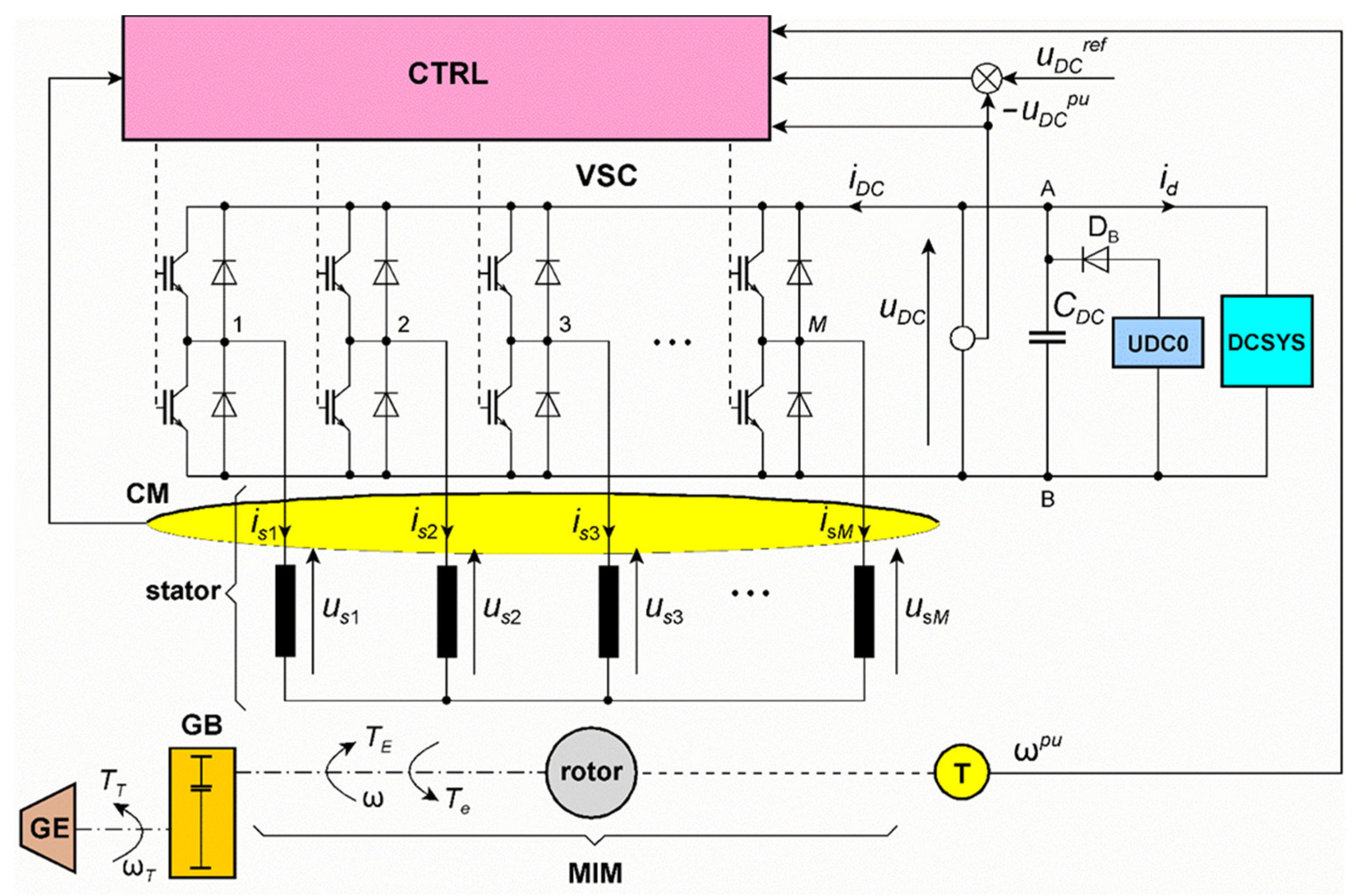
2. Control Properties of a Multiphase Cage Induction Generator

The general structure of the automatic DC voltage control system is shown in Figure 1, where field-oriented vector control was used instead of scalar control, as in [1]. In this paper, the physical basis of the voltage regulation of multiphase cage induction generators is presented.
In the scalar control system (CTRL), the voltage source converter (VSC) was triggered using PWM with sinusoidal control signals:
[ u s 1 p u u s 2 p u u s 3 p u u s k p u u s M p u ] = U s p u [ sin ( ϑ s ) sin ( ϑ s m 2 π M ) sin ( ϑ s 2 m 2 π M ) sin [ ϑ s ( k 1 ) m 2 π M ] sin [ ϑ s ( M 1 ) m 2 π M ] ]
where, for the nine-phase machine, M = 9. The phase angle is as follows:
ϑ s = Ω o 0 t ω s p u d τ
which depends on the stator and rotor p. u. angular frequencies ω s p u and ω r p u , respectively, and the rotor speed ω p u . All of them refer to the base electrical speed Ω o = 2 π f o
ω s p u = m |    ω p u | + ω r p u = f s p u
where f s p u is the stator p. u. frequency referring to the base frequency f o = f s N at the assumed rated frequency, f s N . The numbers m = 0 ,   1 ,   2 ,   3 ,   , M 1 determine the sequence of signals (1) causing M 1 different phase shifts between adjacent signals as an m multiple of 2 π M . The sequence for m = 0 is not useful. The rotor angular frequency, ω r p u , occurring as the output signal of the voltage regulator must be negative to force the generator operation. Thus, it is limited according to ω r p u 0 and ω r p u > ω r max p u .
The p. u. amplitude U s p u was dependent on the angular frequency ω s p u of the stator:
U s p u = { Ψ μ A V p u for ω s p u > 1 Ψ μ A V p u ω s p u for 0 ω s p u 1 0 for ω s p u < 0
and refers to the base voltage U o = U N . For example, at ω p u = 0 and the controller output signal ω r p u < 0 , the signal ω s p u appears as negative according to (3). Then, U s p u must be set to 0 (4). For simplicity, we can assume Ψ μ A V p u = 1 . The sequences m = 1 and 8, 2 and 7, 3 and 6, and 4 and 5 are mutually opposite. Such control caused a change in the sequence of the phase currents and, as a result, a change in the number of pole pairs produced by the nine-phase winding, as is shown in Figure 2. Phase windings of this type are sometimes called asymmetrical because their magnetomotive force (MMF) distribution contains spatial harmonics of the order ν = ( 1 , 2 , 3 , 4 , 5 , ) p , where p —number of pole pairs. This nine-phase winding was defined in [1] as type S = 1, which has quite different properties compared to the winding of type S = 2 ( ν = ( 1 , 3 , 5 , 7 , ) p ). Only windings of the first type are suitable for induction generator operating at varying speed.
Switching the sequence m causes the stator magnetic field to be dominated by a specific harmonic ν = m p producing a different number of pole pairs causing the no-load speeds:
Ω 0 ( + ) = Ω o f s p u m p | m = 1 , 2 , 3 , 4         ;         Ω 0 ( ) = Ω o f s p u ( 9 m ) p | m = 8 , 7 , 6 , 5
The useful sequences for the positive speed direction (5) have the numbers m = 1, 2, 3, 4. For each value of m, the nine-phase generator has a family of different mechanical characteristics, presented in Figure 3 using the colors brown, red, blue, and green. All these characteristics are for the frequency f s = f s N = f o and the same voltage U s p u = 1 . The torque axis is defined for T e p u = T E p u , where T e p u is the machine torque and T E p u is the turbine torque at the output of the mechanical gearbox (GE). This property of switching mechanical characteristics using m is only available for multiphase induction machines with a non-sinusoidal stator winding. The multiphase induction machine with sinusoidally distributed stator winding has the same characteristics for all values of m , i.e., as for m = 1 .
The mechanical characteristics of the generator for each value of m determine the speed ranges in which regulation occurs when changing the frequency f s p u and the amplitude U s p u . This extends the speed range of the generator when the voltage can be kept at a given level. For the family of wind turbine characteristics (black curves for some wind p. u. speeds) the points P1, P2, P3, and P4 of maximum power P E max are shown. The multiphase induction generator can reach these points directly at the rated frequency f s N and sequences m = 2, 4 (P2, P4) or by slightly increasing the stator frequency for a given control sequence (P1 for m = 2, f s = 1.25 f s N , P3 for m = 3, f s = 1.12 f s N ). At the lower power 0.93PEmax the system reaches point P11 when m = 1 and f s = f s N . Thus, the regulation of the sequence number m and the frequency f s enables the generation of the voltage of the desired value while making the best possible use of the driving turbine [21]. This task is to be performed by a vector control system.
The system described in [1] allows, in practice, one to regulate the voltage to a given value with a speed variation of 0.3:1, because at low speeds and an increased number of poles for m = 4 , the magnetizing current reaches high values. The grid-side converter is then supplied with a constant voltage. Its connection to the network and control can be implemented using the methods discussed in [5,13]. When assessing the profitability of use, one can be guided by [22].
Based on the steady-state measurements presented in Section 4, it was demonstrated that the efficiency of the generator operating at low speeds was increased by increasing m and operating with a larger number of poles. This is not possible using the frequency control of an induction generator with a fixed number of poles [2,3,4].

3. Field-Oriented Control with Variable Supply Sequence

3.1. Mathematical Background of Vector Control of a Nine-Phase Generator

The mathematical model of a multiphase squirrel-cage induction machine taking into account the influence of higher spatial harmonics is sufficiently complex [23,24] such that it does not enable the direct formulation of the field-oriented control law. It must be simplified in such a way as to express all the main features of the machine and at the same time enable the construction of a control system. The mathematical model of a multiphase squirrel-cage induction machine is presented below and, by making justified simplifications, a system of equations was formulated that allows for the implementation of vector control in a similar way to monoharmonic machines.
The system of voltage equations of a multiphase squirrel-cage induction machine described in machine coordinates is presented below.
[ U s 1 0 ] = [ R s 1 0 0 R r 1 ] [ I s 1 I r 1 ] + d d t [ L σ s 1 + L s 1 M s r 1 M s r 1 T L σ r 1 + L r 1 ] [ I s 1 I r 1 ]
The number of stator equations is equal to the number of phases M = 9, while the number of rotor equations is equal to the number of cage meshes N, where each mesh is created by two bars and two end ring segments. U s 1 = [ u s 1 , u s 2 , u s 3 , , u s 9 ] T and I s 1 = [ i s 1 , i s 2 , i s 3 , , i s 9 ] T are the vectors of the phase voltages and phase currents, respectively (the superscript T is the transposition index). I r 1 = [ i r 1 , i r 2 , i r 3 , , i r N ] T is the vector of the cage mesh currents. The matrices of the stator resistances R s 1 and leakage inductances L σ s 1 are usually diagonal (when neglecting mutual coupling between phases due to leakage fluxes). The matrix of the rotor resistances R r 1 and the matrix L σ r 1 of the rotor leakage inductances incorporate self and mutual elements among adjacent cage meshes. In the matrix M s r 1 of the mutual inductances between the stator and rotor circuits are coded the main features of the multiphase machine. Each inductance is a function of the rotor rotation angle φ as a sum of the harmonic inductances depending on the number of MMF harmonics taken into account. The orders of these spatial harmonics are given below [1]:
ν = ν / p    ;      ν / = 1 , 2 , 3 , 4 , 5 ,
The stator and the rotor winding matrices of the self and mutual inductances L s 1 and L r 1 have parameters directly connected with matrix M s r 1 .
After transforming into a vector form in symmetric components, the voltage equations of the machine take the following form:
[ U s 2 0 ] = [ R s 2 0 0 R r 2 ] [ I s 2 I r 2 ] + [ L σ s 2 + L s 2 0 0 L σ r 2 + L r 2 ]    d d t [ I s 2 I r 2 ] + d d t    [ 0 M s r 2 M s r 2 * 0 ] [ I s 2 I r 2 ]
where
U s 2 = S s U s 1 = [ u _ s ( 0 ) u _ s ( 1 ) = u s α ( 1 ) + j u s β ( 1 ) u _ s ( 2 ) = u s α ( 2 ) + j u s β ( 2 ) u _ s ( 3 ) = u s α ( 3 ) + j u s β ( 3 ) u _ s ( 4 ) = u s α ( 4 ) + j u s β ( 4 ) u _ s ( 4 ) * = u s α ( 4 ) j u s β ( 4 ) u _ s ( 3 ) * = u s α ( 3 ) j u s β ( 3 ) u _ s ( 2 ) * = u s α ( 2 ) j u s β ( 2 ) u _ s ( 1 ) * = u s α ( 1 ) j u s β ( 1 ) ] ;    I s 2 = S s I s 1 = [ i _ s ( 0 ) i _ s ( 1 ) = i s α ( 1 ) + j i s β ( 1 ) i _ s ( 2 ) = i s α ( 2 ) + j i s β ( 2 ) i _ s ( 3 ) = i s α ( 3 ) + j i s β ( 3 ) i _ s ( 4 ) = i s α ( 4 ) + j i s β ( 4 ) i _ s ( 4 ) * = i s α ( 4 ) j i s β ( 4 ) i _ s ( 3 ) * = i s α ( 3 ) j i s β ( 3 ) i _ s ( 2 ) * = i s α ( 2 ) j i s β ( 2 ) i _ s ( 1 ) * = i s α ( 1 ) j i s β ( 1 ) ] ;    I r 2 = S r I r 1 = [ i _ r ( 0 ) i _ r ( 1 ) = i r d ( 1 ) + j i r q ( 1 ) i _ r ( 2 ) = i r d ( 2 ) + j i r q ( 2 ) i _ r ( 3 ) = i r d ( 3 ) + j i r q ( 3 ) i _ r ( 4 ) = i r d ( 4 ) + j i r q ( 4 ) i _ r ( 5 ) = i r d ( 5 ) + j i r q ( 5 ) i _ r ( 5 ) * = i r d ( 5 ) j i r q ( 5 ) i _ r ( 4 ) * = i r d ( 4 ) j i r q ( 4 ) i _ r ( 3 ) * = i r d ( 3 ) j i r q ( 3 ) i _ r ( 2 ) * = i r d ( 2 ) j i r q ( 2 ) i _ r ( 1 ) * = i r d ( 1 ) j i r q ( 1 ) ]
*—conjugation index. The transformation matrices are described as follows:
S 9 = 2 9 [ 1 1 1 1 1 a _ 1 a _ 2 a _ 8 1 a _ 2 a _ 4 a _ 16 1 1 a _ 8 a _ 16 a _ 64 ] ; a _ = e j 2 π / 9   ; S r = 2 N [ 1 1 1 1 1 1 b _ 1 b _ 2 b _ 3 b _ ( N 1 ) 1 b _ 2 b _ 4 b _ 6 b _ 2 ( N 1 ) 1 b _ 3 b _ 6 b _ 9 b _ 3 ( N 1 ) 1 1 b _ ( N 1 ) b _ 2 ( N 1 ) b _ 3 ( N 1 ) b _ ( N 1 ) 2 ] ; b _ = e j 2 π / N
M s r 2   is a full matrix of dimension 9 × N , shown below in the general form:
M s r 2   = [ M _ 0 , 0 M _ 0 , 1 M _ 0 , 2 M _ 0 , 3 M _ 0 , 4           M _ 1 , 0 M _ 1 , 1 M _ 1 , 2 M _ 1 , 3 M _ 1 , 4           M _ 2 , 0 M _ 2 , 1 M _ 2 , 2 M _ 2 , 3 M _ 2 , 4         M _ 3 , 0 M _ 3 , 1 M _ 3 , 2 M _ 3 , 3 M _ 3 , 4           M _ 4 , 0 M _ 4 , 1 M _ 4 , 2 M _ 4 , 3 M _ 4 , 4       M _ W , K   M _ 5 , 5                     M _ 6 , 6           M _ 7 , 7       M _ 8 , 0 M _ 8 , 1 M _ 8 , 2 M _ 8 , 3 M _ 8 , 4     M _ 8 , 8                 M _ 0 , 4 * M _ 0 , 3 * M _ 0 , 2 * M _ 0 , 1 *       M _ 8 , 8 *     M _ 8 , 4 * M _ 8 , 3 * M _ 8 , 2 * M _ 8 , 1 *       M _ 7 , 7 *             M _ 6 , 6 *             M _ W , K *     M _ 5 , 5 *           M _ 4 , 4 * M _ 4 , 3 * M _ 4 , 2 * M _ 4 , 1 *         M _ 3 , 4 * M _ 3 , 3 * M _ 3 , 2 * M _ 3 , 1 *           M _ 1 , 4 * M _ 2 , 3 * M _ 2 , 2 * M _ 2 , 1 *           M _ 1 , 4 * M _ 1 , 3 * M _ 1 , 2 * M _ 1 , 1 * ]
The inductances of this matrix are described by the expression:
M _ W , K = ν / M ( ν / ) e ± j ν / p φ ;    W = 0 , 1 , 2 , , 8 ;    K = 0 , 1 , 2 , , N 1
where W is the number of the matrix row and K is the number of the matrix column, and additionally, these are the numbers of the stator and rotor symmetric components, respectively. For all the harmonic orders given by (7),
W = ( ± ν / ) mod 9 ;    K = ( ± ν / p ) mod N
M   ( ν / ) = 9 N μ 0 d c l c π δ N s k s ( ν / ) k r ( ν / ) k skew ( ν / ) ( ν / p ) 2
where μ 0 = 4 π · 10 7 H/m, d c —stator inside diameter, l c —equivalent length of the machine core, δ —air gap equivalent length comprising the Carter’s factor, N s —number of stator phase turns, k s ν / , k r ν / —winding factors for the stator and the rotor, respectively, k skew ν / —skew factor.
Matrix M s r 2   can be presented in the simplified form when N > 3M (M = 9). For a symmetrical machine with a star connection of the stator, the terms of the M s r 2   matrix lying in the W = 0 row and K = 0 column have no importance and can be omitted. Thus, the zero components of vectors I s 2 and I r 2 in (9) have no importance. The fundamental simplification is that the most important terms (12) of the M s r 2   matrix are taken into account. These are the terms: M 1 , 1 , M 2 , 2 , M 3 , 3 , M 4 , 4 , M 5 , 5 , M 6 , 6 , M 7 , 7 , M 8 , 8 , M 1 , 10 , M 2 , 11 , M 3 , 12 , M 4 , 13 , …, M W 0 , K 0 , where K 0 = N 2 1 for even N or K 0 = N 1 2 for odd N . This means that the harmonic orders of the field have been limited to
ν / = 1 , 2 , 3 , 4 , 5 , 6 , 7 , , ν max /
where ν max / = K 0 and the row number W 0 of the last term M W 0 , K 0 is given by (13) for ν max / . For example, when N = 28 , then K 0 = 13 and W 0 = 4. With more rotor bars N , the same harmonic limit can be assumed for most machines. Despite such simplifications, the multiphase induction machine model retains all its most important properties. In such a case, the M s r 2   matrix can be represented as
M s r 2   = L μ N s r 1 K R
where matrix L μ has the dimension ( M 1 ) × 2 K 0 :
L μ = [ L μ ( 1 )               L μ ( 10 )         L μ ( 2 )               L μ ( 11 )         L μ ( 3 )               L μ ( 12 )         L μ ( 4 )               L μ ( 13 )         L μ ( 5 )                         L μ ( 6 )                         L μ ( 7 )                         L μ ( 8 )                 L μ ( 8 )                         L μ ( 7 )                         L μ ( 6 )                         L μ ( 5 )         L μ ( 13 )               L μ ( 4 )         L μ ( 12 )               L μ ( 3 )         L μ ( 11 )               L μ ( 2 ) L 2         L μ ( 10 )               L μ ( 1 ) ] = [ L μ A 1 L μ B 1 L μ A 2 L μ B 2 ]
from which
L μ A 1 = [ L μ ( 1 )               L μ ( 10 )         L μ ( 2 )               L μ ( 11 )         L μ ( 3 )               L μ ( 12 )         L μ ( 4 )               L μ ( 13 ) ]
L μ B 1 = [         L μ ( 8 )                         L μ ( 7 )                         L μ ( 6 )                         L μ ( 5 )         ]
L μ A 2 = [         L μ ( 5 )                         L μ ( 6 )                         L μ ( 7 )                         L μ ( 8 )         ]
L μ B 2 = [ L μ ( 13 )               L μ ( 4 )         L μ ( 12 )               L μ ( 3 )         L μ ( 11 )               L μ ( 2 )         L μ ( 10 )               L μ ( 1 ) ]
and
N s r - 1 = diag [ 1 ξ ( 1 ) , 1 ξ ( 2 ) , 1 ξ ( 3 ) , 1 ξ ( 4 ) , 1 ξ ( 5 ) , 1 ξ ( 6 ) , 1 ξ ( 7 ) , 1 ξ ( 8 ) , 1 ξ ( 10 ) , 1 ξ ( 11 ) , 1 ξ ( 12 ) , 1 ξ ( 13 ) ,                                1 ξ ( 13 ) , 1 ξ ( 12 ) , 1 ξ ( 11 ) , 1 ξ ( 10 ) , 1 ξ ( 8 ) , 1 ξ ( 7 ) , 1 ξ ( 6 ) , 1 ξ ( 5 ) , 1 ξ ( 4 ) , 1 ξ ( 3 ) , 1 ξ ( 2 ) , 1 ξ ( 1 ) ]
K R = diag [ e j p φ , e j 2 p φ , e j 3 p φ , e j 4 p φ , e j 5 p φ , e j 6 p φ , e j 7 p φ , e j 8 p φ , e j 10 p φ , e j 11 p φ , e j 12 p φ , e j 13 p φ ,                             e j 13 p φ , e j 12 p φ , e j 11 p φ , e j 10 p φ , e j 8 p φ , e j 7 p φ , e j 6 p φ , e j 5 p φ , e j 4 p φ , e j 3 p φ , e j 2 p φ , e j p φ ]
The above expressions do not contain elements for the harmonic order ν / = 9 , because the inductance (14) for this harmonic belongs to the W = 0 row of the M s r 2   matrix.
The magnetizing inductances in (17) are described with the following formula:
L μ ( ν / ) = 9 μ 0 d c l c π δ ( N s k s ( ν / ) ν / p ) 2
where ν / is given by (15). For the same orders ν / , the current ratios between the stator and rotor windings in (22) are given by
ξ ( ν / ) = 9 N N s k s ( ν / ) k r ( ν / ) k skew ( ν / )
The vector rotation matrix (23) also depends on harmonic orders ν / .
Now, the vector I r 2 of the symmetric components of the rotor currents (9) is transformed into the stationary reference frame (α-β), associated with the stator, according to the following transformation:
I r 3 = N s r 1 K R I r 2 = I r 3 A I r 3 B = = i _ r / ( 1 ) , i _ r / ( 2 ) , i _ r / ( 3 ) , i _ r / ( 4 ) , i _ r / ( 5 ) , i _ r / ( 6 ) , i _ r / ( 7 ) , i _ r / ( 8 ) , i _ r / ( 10 ) , i _ r / ( 11 ) , i _ r / ( 12 ) , i _ r / ( 13 ) T i _ r / ( 13 ) * , i _ r / ( 12 ) * , i _ r / ( 11 ) * , i _ r / ( 10 ) * , i _ r / ( 8 ) * , i _ r / ( 7 ) * , i _ r / ( 6 ) * , i _ r / ( 5 ) * , i _ r / ( 4 ) * , i _ r / ( 3 ) * , i _ r / ( 2 ) * , i _ r / ( 1 ) * T
Generally,
i _ r / ( k ) = i r α ( k ) + j i r β ( k )    ;     k = 1 , 2 , 3 , , 13
The numbers k denote the numbers of the rotor’s symmetrical components and are also the harmonic orders ν / in the inductance matrix (17). The set of voltage equations assumes the following form:
[ U s 3 A U s 3 B 0 0 ] = [ R s 3 A         R s 3 B         R r 3 A         R r 3 B ] [ I s 3 A I s 3 B I r 3 A I r 3 B ] + d d t [ Ψ s 3 A Ψ s 3 B Ψ r 3 A Ψ r 3 B ] j p ω [ 0         0         K A         K B ] [ 0 0 Ψ r 3 A Ψ r 3 B ]
The vectors and matrices of these voltage equations are as follows:
For the stator:
U s 3 A = [ u _ s ( 1 ) , u _ s ( 2 ) , u _ s ( 3 ) , u _ s ( 4 ) ] T    ;     U s 3 B = [ u _ s ( 4 ) * , u _ s ( 3 ) * , u _ s ( 2 ) * , u _ s ( 1 ) * ] T
I s 3 A = [ i _ s ( 1 ) , i _ s ( 2 ) , i _ s ( 3 ) , i _ s ( 4 ) ] T    ;           I s 3 B = [ i _ s ( 4 ) * , i _ s ( 3 ) * , i _ s ( 2 ) * , i _ s ( 1 ) * ] T
Ψ s 3 A = [ ψ _ s ( 1 ) , ψ _ s ( 2 ) , ψ _ s ( 3 ) , ψ _ s ( 4 ) ] T    ;     Ψ s 3 B = [ ψ _ s ( 4 ) * , ψ _ s ( 3 ) * , ψ _ s ( 2 ) * , ψ _ s ( 1 ) * ] T
R s 3 A = R s 3 B = diag [ R s , R s , R s , R s ]
For the rotor:
Ψ r 3 A   = [ ψ _ r / ( 1 ) , ψ _ r / ( 2 ) , ψ _ r / ( 3 ) , ψ _ r / ( 4 ) , ψ _ r / ( 5 ) , ψ _ r / ( 6 ) , ψ _ r / ( 7 ) , ψ _ r / ( 8 ) , ψ _ r / ( 10 ) , ψ _ r / ( 11 ) , ψ _ r / ( 12 ) , ψ _ r / ( 13 ) ] T Ψ r 3 B   = [ ψ _ r / ( 13 ) * , ψ _ r / ( 12 ) * , ψ _ r / ( 11 ) * , ψ _ r / ( 10 ) * , ψ _ r / ( 8 ) * , ψ _ r / ( 7 ) * , ψ _ r / ( 6 ) * , ψ _ r / ( 5 ) * , ψ _ r / ( 4 ) * , ψ _ r / ( 3 ) * , ψ _ r / ( 2 ) * , ψ _ r / ( 1 ) * ] T    }
R r 3 A   = diag [ R r ( 1 ) , R r ( 2 ) , R r ( 3 ) , R r ( 4 ) , R r ( 5 ) , R r ( 6 ) , R r ( 7 ) , R r ( 8 ) , R r ( 10 ) , R r ( 11 ) , R r ( 12 ) , R r ( 13 ) ] R r 3 B   = diag [ R r ( 13 ) , R r ( 12 ) , R r ( 11 ) , R r ( 10 ) , R r ( 8 ) , R r ( 7 ) , R r ( 6 ) , R r ( 5 ) , R r ( 4 ) , R r ( 3 ) , R r ( 2 ) , R r ( 1 ) ]    }
K A   = diag [ 1 ,    2 ,    3 ,    4 ,    5 ,    6 ,    7 ,    8 ,    10 ,    11 ,    12 ,    13 ] K B   = diag [ 13 , 12 , 11 , 10 , 8 , 7 , 6 , 5 , 4 , 3 , 2 , 1 ]    }
The relationships of the flux vectors coupled to the current vectors are shown below.
[ Ψ s 3 A Ψ s 3 B Ψ r 3 A Ψ r 3 B ] = [ L s 3 A 0 L μ A 1 L μ B 1 0 L s 3 B L μ A 2 L μ B 2 L μ A 1 T L μ A 2 T L r 3 A 0 L μ B 1 T L μ B 2 T 0 L r 3 B ] [ I s 3 A I s 3 B I r 3 A I r 3 B ]
L s 3 A = diag [ L σ s + L s ( 1 ) , L σ s + L s ( 2 ) , L σ s + L s ( 3 ) , L σ s + L s ( 4 ) ] L s 3 B = diag [ L σ s + L s ( 4 ) , L σ s + L s ( 3 ) , L σ s + L s ( 2 ) , L σ s + L s ( 1 ) ] }
L s ( 1 ) = L μ ( 1 ) + L μ ( 10 ) + L μ ( 8 ) ;    L s ( 2 ) = L μ ( 2 ) + L μ ( 11 ) + L μ ( 7 ) L s ( 3 ) = L μ ( 3 ) + L μ ( 12 ) + L μ ( 6 ) ;    L s ( 4 ) = L μ ( 4 ) + L μ ( 13 ) + L μ ( 5 )
L r 3 A = diag [ L r ( 1 ) , L r ( 2 ) , L r ( 3 ) , L r ( 4 ) , L r ( 5 ) , L r ( 6 ) , L r ( 7 ) , L r ( 8 ) , L r ( 10 ) , L r ( 11 ) , L r ( 12 ) , L r ( 13 ) ] L r 3 B = diag [ L r ( 13 ) , L r ( 12 ) , L r ( 11 ) , L r ( 10 ) , L r ( 8 ) , L r ( 7 ) , L r ( 6 ) , L r ( 5 ) , L r ( 4 ) , L r ( 3 ) , L r ( 2 ) , L r ( 1 ) ] }
For numbers k of the rotor symmetrical components,
L r ( k ) = L σ r ( k ) + L μ ( k )
L σ r ( k ) = [ 2 L G + 4 L B sin 2 ( k p π N ) ] ( ξ   ( k ) ) 2 + L μ ( k ) ( 1 ( k skew ( k ) ) 2 1 )
R r ( k ) = [ 2 R G + 4 R B sin 2 ( k p π N ) ] ( ξ   ( k ) ) 2
When using PWM to control the VSC with signals (1), impulse voltages will occur at the stator terminals, the averaged waveforms of which (the fundamental time-harmonics) take the following form:
U s 1 = [ u s 01   u s 02   u s 03   u s 0 k p u ] = U S   [ sin ( ϑ s ) sin ( ϑ s m 2 π 9 ) sin ( ϑ s 2 m 2 π 9 ) sin [ ϑ s 8 m 2 π 9 ] ]
These voltages take on a vector form U s 2 after being transformed into symmetrical components:
U s 2 = S s U s 1 = [ u _ s ( 1 ) u _ s ( 2 ) u _ s ( 3 ) u _ s ( 4 ) u _ s ( 5 ) u _ s ( 6 ) u _ s ( 7 ) u _ s ( 8 ) ] = [ u _ s ( 1 ) u _ s ( 2 ) u _ s ( 3 ) u _ s ( 4 ) u _ s ( 4 ) * u _ s ( 3 ) * u _ s ( 2 ) * u _ s ( 1 ) * ]    =    1 j U S { [ 0 0 c ( W ) 0 0 ] e j ϑ s [ 0 0 0 c ( W ) 0 ] e j ϑ s } = [ U s 3 A U s 3 B ]
where for m = 1, 2, 3, …, 8, W =    1 ,    2 , , 8 and
c ( W ) = 1    for    W = m c ( W ) = 0    for    W m }
(sequence number m = 0 is useless). This means that there are only two non-zero symmetric components in the vector U s 2 , which are conjugate numbers. This property is used to simplify the mathematical model of a multiphase machine in order to formulate the principle of vector control for various sequence numbers m. Hence, the voltage vectors U s 3 A , U s 3 B of Equation (28) have only one non-zero element for a given m = 1 , 2 , 3 , 4 , 5 , 6 , 7 , 8 . For example, for m = 2 , this voltage vector has the following form:
U s 3 A = [ u _ s ( 1 ) u _ s ( 2 ) u _ s ( 3 ) u _ s ( 4 ) ] = [ 0 u _ s ( 2 ) 0 0 ] = 1 j U S e j ϑ s    ;     U s 3 B = [ u _ s ( 4 ) * u _ s ( 3 ) * u _ s ( 2 ) * u _ s ( 1 ) * ] = [ 0 0 u _ s ( 2 ) * 0 ] = 1 j U S e j ϑ s
whereas for m = 7 ,
U s 3 A = [ u _ s ( 1 ) u _ s ( 2 ) u _ s ( 3 ) u _ s ( 4 ) ] = [ 0 u _ s ( 2 ) 0 0 ] = 1 j U S e j ϑ s    ;     U s 3 B = [ u _ s ( 4 ) * u _ s ( 3 ) * u _ s ( 2 ) * u _ s ( 1 ) * ] = [ 0 0 u _ s ( 2 ) * 0 ] = 1 j U S e j ϑ s
The pairs of mutually conjugated symmetrical components in U s 3 A and U s 3 B , I s 3 A and I s 3 B , and in the transformed rotor current vector I r 3 A   and I r 3 B   carry the same information. Hence, the number of voltage equations is two times lower.
In fact, all the symmetric components u _ s ( 1 ) , u _ s ( 2 ) , u _ s ( 3 ) , u _ s ( 4 ) are non-zero, because each higher time-harmonic of the inverter output voltage excites them. However, the influence of these higher harmonics has only a parasitic effect to an almost negligible extent. So, such a property can be utilized to separate this stator voltage equations for which u _ s ( m ) 0 . Taking into account only the spatial harmonics ν / = m for m = 1, 2, 3, 4, the system of machine Equation (28) takes a simple form, corresponding to machines with sinusoidal windings for each m and which is described in the stationary reference frame (α-β), where in matrices K A and K B , the values m and m are only taken, respectively:
[ u _ s ( m ) 0 ] = [ R s       R r ( m ) ] [ i _ s ( m ) i _ r ( m ) ] + d d t [ ψ _ s ( m ) ψ _ r ( m ) ] j m p ω [ ψ _ s ( m ) ψ _ r ( m ) ]
Flux vectors:
[ ψ _ s ( m ) ψ _ r ( m ) ] = [ L σ s + L μ ( m ) L μ ( m ) L μ ( m ) L σ r ( m ) + L μ ( m ) ] [ i _ s ( m ) i _ r ( m ) ]
This means that only the single symmetric components i _ s ( m ) and i _ r ( m ) are taken into account. These components are coupled through one mutual (magnetizing) inductance L μ ( ν / ) = L μ ( m ) (24) for a given m = ν / . This makes it possible to use vector control methods known for three-phase induction machines with the squirrel-cage [3]; however, this is taking into account the operation at a given value of m , which determines the number of pole pairs m   p . One must be aware that the actual parameters of the machine are slightly different than in the model adopted for control.

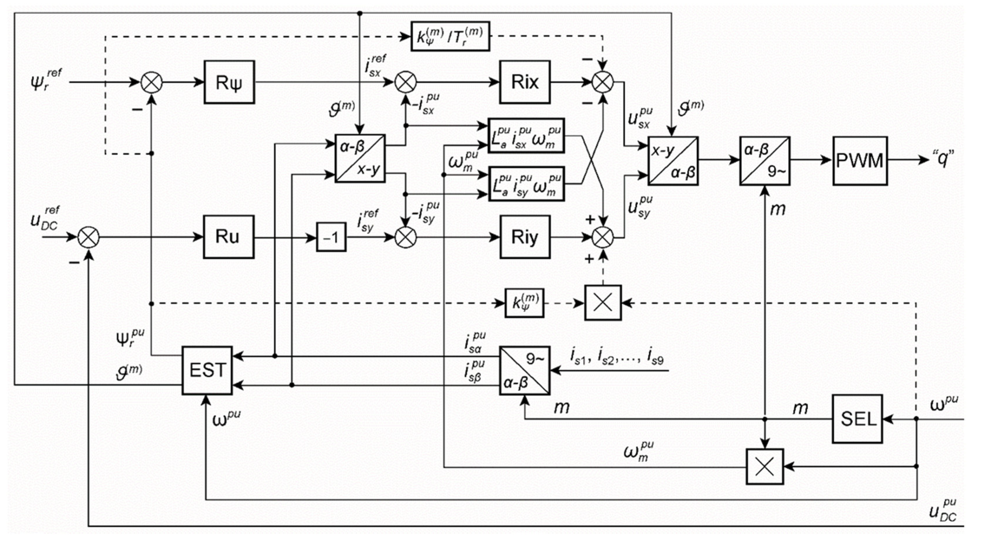
3.2. Field-Oriented Control System of the Generator

Field-oriented control was implemented with respect to the rotor flux vector ψ _ r ( m ) . The ϑ ( m ) position of this vector in the stationary reference frame (α-β) determines the rotating reference frame (x(m)-y(m)). Additionally, the coordinate system (d-q) of the rotor is rotating with the rotor rotation angle φ relative to the stator. This is shown in Figure 4.
Based on (47), the vectors ψ _ s ( m ) and i _ r ( m ) should be eliminated from Equation (46). The obtained stator and rotor equations after separating the real and imaginary parts, due to Euler’s identity, take the form which allows for the control scheme formulation. These equations described in the rotating reference frame (x(m)-y(m)) assume the following form:
For the stator:
u s x ( m ) = R a ( m ) ( i s x ( m ) + T a ( m ) d d t i s x ( m ) ) + e s x ( m )    ;      e s x ( m ) = L a ( m ) i s y ( m ) ω ( m ) k Ψ ( m ) ψ r x ( m ) / T r ( m )
u s y ( m ) = R a ( m ) ( i s y ( m ) + T a ( m ) d d t i s y ( m ) ) + e s y ( m )    ;      e s y ( m ) = m p k Ψ ( m ) ψ r x ( m ) ω + L a ( m ) i s x ( m ) ω ( m )
For the rotor:
i s x ( m ) = 1 L μ ( m ) ( ψ r x ( m ) + T r ( m ) d d t ψ r x ( m ) )
d d t ϑ ( m ) = ω ( m ) = 1 T r ( m ) L m ψ r x ( m ) i s y ( m ) + m p ω
where
L s ( m ) = L σ s + L μ ( m )    ;    L r ( m ) = L σ r ( m ) + L μ ( m ) k Ψ ( m ) = L μ ( m ) L r ( m )    ;     R a ( m ) = R s + R r ( m ) ( k Ψ ( m ) ) 2    ;     L a ( m ) = L s ( m ) L r ( m ) ( L μ ( m ) ) 2 L r ( m ) T a ( m ) = L a ( m ) R a ( m )    ;      T r ( m ) = L r ( m ) R r ( m )
For the coordinates of the stator voltage and current vectors and the rotor flux vector, the transformation between reference frames (α-β), (x(m)-y(m)), and (d-q) is orthogonal:
[ z x z y ] = [ cos ϑ ( m ) sin ϑ ( m ) sin ϑ ( m ) cos ϑ ( m ) ] [ z α z β ]    ;      [ z d z q ] = [ cos φ sin φ sin φ cos φ ] [ z α z β ]
where instead of z , substitute the appropriate symbol for the voltage, current, and flux.
The machine electromagnetic torque of the above simplified model is described by the following equation:
T e ( m ) = 9 2    p    m    k Ψ ( m ) ψ r x ( m ) i s y ( m )
The following basic reference units were assumed:
  • Ω o = 2 π f o    ;      f o = f s N ;
  • U o = 2 U s N ; U s N —r. m. s value of rated phase voltage;
  • I o = 2 I s N ; I s N —r. m. s value of rated phase current.
The control system signals were determined in the form of relative values (per unit) of the speed, stator voltage, stator current, and the rotor flux referred to Ψ o = U o Ω o . The per unit speeds were as follows:
ω p u = p ω Ω o    ;      ω m p u = ω ( m ) Ω o
Additionally, the resistances and inductances also referred to the basic resistance R o = U o / I o and inductance L o = Ψ o / I o respectively. The remaining per unit quantities (stator voltage, stator current components, rotor flux) are defined as follows:
u s x p u = u s x ( m ) / U o ;    u s y p u = u s y ( m ) / U o ;    i s x p u = i s x ( m ) / I o ;    i s y p u = i s y ( m ) / I o ;    ψ r p u = ψ r x ( m ) / Ψ o
For the basic unit of the torque T o = 9 2 p U o I o Ω o = 9 p U s N I s N 2 π f s N , the electromagnetic torque (54) takes the following per unit form:
T e p u = m    k Ψ ( m ) ψ r p u i s y p u
Following the presented equations, the control scheme has been formulated and is presented in Figure 5. The estimation of the modulus of the rotor flux vector ψ _ r ( m ) and the ϑ ( m ) angle of the (x(m)-y(m)) reference frame is performed in the EST block. The structure of this block is shown in Figure 6. This results directly from (46) and (47) for the rotor p. u. equation described in the d-q reference frame: d d t ψ _ r ( m ) p u = Ω o T r ( m ) ( L μ ( m ) p u i _ s ( m ) p u ψ _ r ( m ) p u ) .
The blocks of orthogonal transformation between the reference systems (α-β)/(x(m)-y(m)), (α-β)/(d-q) for the systems of Figure 5 and Figure 6 are described by the relationships of (53). The nine-phase system of currents is transformed to the vector form i _ s ( m ) using the transformation resultant from matrix S 9 (10):
[ i s α p u i s β p u ] = 2 9 [ 1 cos m 2 π 9 cos 2 m 2 π 9 cos 3 m 2 π 9 cos 7 m 2 π 9 cos 8 m 2 π 9 0 sin m 2 π 9 sin 2 m 2 π 9 sin 3 m 2 π 9 sin 7 m 2 π 9 sin 8 m 2 π 9 ] [ i s 1 p u i s 2 p u i s 3 p u i s 4 p u i s 8 p u i s 9 p u ]
The control paths x and y in Figure 5 are decoupled using signals e s x ( m ) p u and e s y ( m ) p u added to the outputs of the current controllers Rix and Riy. They result from Equations (48) and (49). This decoupling can be simplified by assuming a constant value of ψ r p u and ignoring the signals connected in Figure 5 by the dashed lines. This is justified additionally by the small derivative of the speed signal ω p u compared to the derivative of the signal i s y p u .
In the SEL block, the value of m is selected as a function of the generator speed. Switching the control sequence m was implemented with hysteresis:
k m 2 = [ 1 + sgn ( Ω 1 , 2 p u ω p u + H k m 2 ) ] / 2 k m 3 = [ 1 + sgn ( Ω 2 , 3 p u ω p u + H k m 3 ) ] / 2 k m 4 = [ 1 + sgn ( Ω 3 , 4 p u ω p u + H k m 4 ) ] / 2 m = 1 + k m 2 + k m 3 + k m 4     }
where the “sgn” function is treated as an ideal comparator for H = 0.1—half of the hysteresis. Based on the mechanical characteristics from Figure 3, it was assumed that Ω 1 , 2 p u = 1 / 2 , Ω 2 , 3 p u = 1 / 3 , Ω 3 , 4 p u = 1 / 4 .
The nine-phase induction generator is the same as presented in [1]. The magnetic core was taken from 4 kW induction machine (Sf112M-4) where the nine-phase winding (Figure 2) was applied. The cage rotor has 28 aluminium bars. Parameters: M = 9, p = 1, μ 0 = 4 π · 10 7 H/m, d c = 0.11 m, l c = 0.12 m, N s = 110. For safety reasons, the ratings have been reduced relative to the potential capabilities of the machine: P N = 1 kW, U s N = 67.5 V, I s N = 5.3 A, p = 1, f s N = 33.3 Hz. The average flux (4): Ψ μ A V   = U s N / 2 π f s N = 0.322 Wb. Hence, the basic reference units are Ω o = 209.2 rad/s (2000 rev/min), I o = 7.5 A, U o = 95.4 V, P o = 9 2 U o I o = 3219 W, T o = P o Ω o = 15.4 Nm. The parameters of the mathematical model and for the control system (Figure 5 and Figure 6) are presented in Table 1.
The voltage (Ru), flux (Rψ), and current (Rix, Riy) controllers are of type PIsat (PI with saturation). The reference voltage signal is u D C r e f = 1.57, which corresponds to the DC voltage u D C = π 2 U s N = 150 V. The rotor flux command signal is Ψ r r e f = 0.701. This corresponds to Ψ μ A V   = 0.322 Wb.
The parameters of the controllers were initially selected using Kessler’s criteria and then modified in practice.
Voltage controller Ru (PIsat):
  • Controller gain K U p u = 5.
  • Time constant T u = 0.1 s.
  • Saturation I s y max p u = 1.
Flux controller Rψ (PIsat):
  • Controller gain K Ψ p u = 1 2 1 L μ ( m ) = 0.108 (m = 1), 0.147 (m = 2), 0.258 (m = 3),
  • 0.648 (m = 4).
  • Time constant T Ψ = T r ( m ) = 0.624 s (m = 1), 0.230 s (m = 2), 0.120 s (m = 3),
  • 0.071 s (m = 4).
  • Saturation I s x max p u = 1.
Current controllers Rix and Riy (PIsat):
Controller gains K I x p u = K I y p u = S K I R a ( m ) p u 2 . For S K I ≈ 30 and similar resistance values for each m, the average value was assumed:   K I x p u = K I y p u = 2.25.
Time constant. To speed up the regulation, the time constant was selected according to the Kessler symmetry criterion. This causes the capacitor C D C to charge faster. For the frequency f c = 3 kHz of VSC (Figure 1), the digital control system performed at twice the switching frequency, synchronously with the carrier signal. Hence, the sampling frequency f s a m p = 2 f c = 6 kHz. The time delay is T d e l = 1 / f s a m p . So, the so-called short time constant of the object inertia can be assumed T σ = 1.5 T d e l . Thus, the time constant of the controller was set to T I = 4 T σ = 1 ms for each m .
An analysis of the differences between the compete mathematical model and the simplified one allows the designer to consciously influence the regulator settings and the structure of the control system in the event of disturbances or a poorer quality of work.

4. Laboratory Tests of the Generation System

4.1. Description of the Laboratory Stand

The laboratory stand was almost the same as presented and described in [1] for the scalar control of the nine-phase induction generator. The main difference was the vector control method implemented for the digital signal controller. All the main tracks of the measurement system and signal transmission are related to the diagram shown in Figure 1. The speed of the MIM operating as a generator was set by a DC motor powered by a rectifier. The mechanical connection was made using the DATAFLEX 32/300 torque meter enabling the measurement of the generator torque T e , as well as the speed ω and rotation angle φ using the quadrature encoder 720 imp/rev with the speed sensor. The phase currents i s 1 , i s 2 , , i s 9 were measured using the Chauvin Arnoux E3N probe, whereas the DC voltage u D C was measured using the TESTEC TT-SI 9001 probe. The measured signals were transmitted through a data acquisition card from National Instruments USB-6211. The control system was based on a digital signal controller from Texas Instruments TMS320F28379D. The VSC was made of a IGBT modules Mitsubishi CM50DY-24H with the gate drivers of our own design. The DCSYS was made as a DC chopper supplying the Rd-Ld load blocked with the freewheeling diode (Rd = 8.5 Ω, Ld = 15 mH).

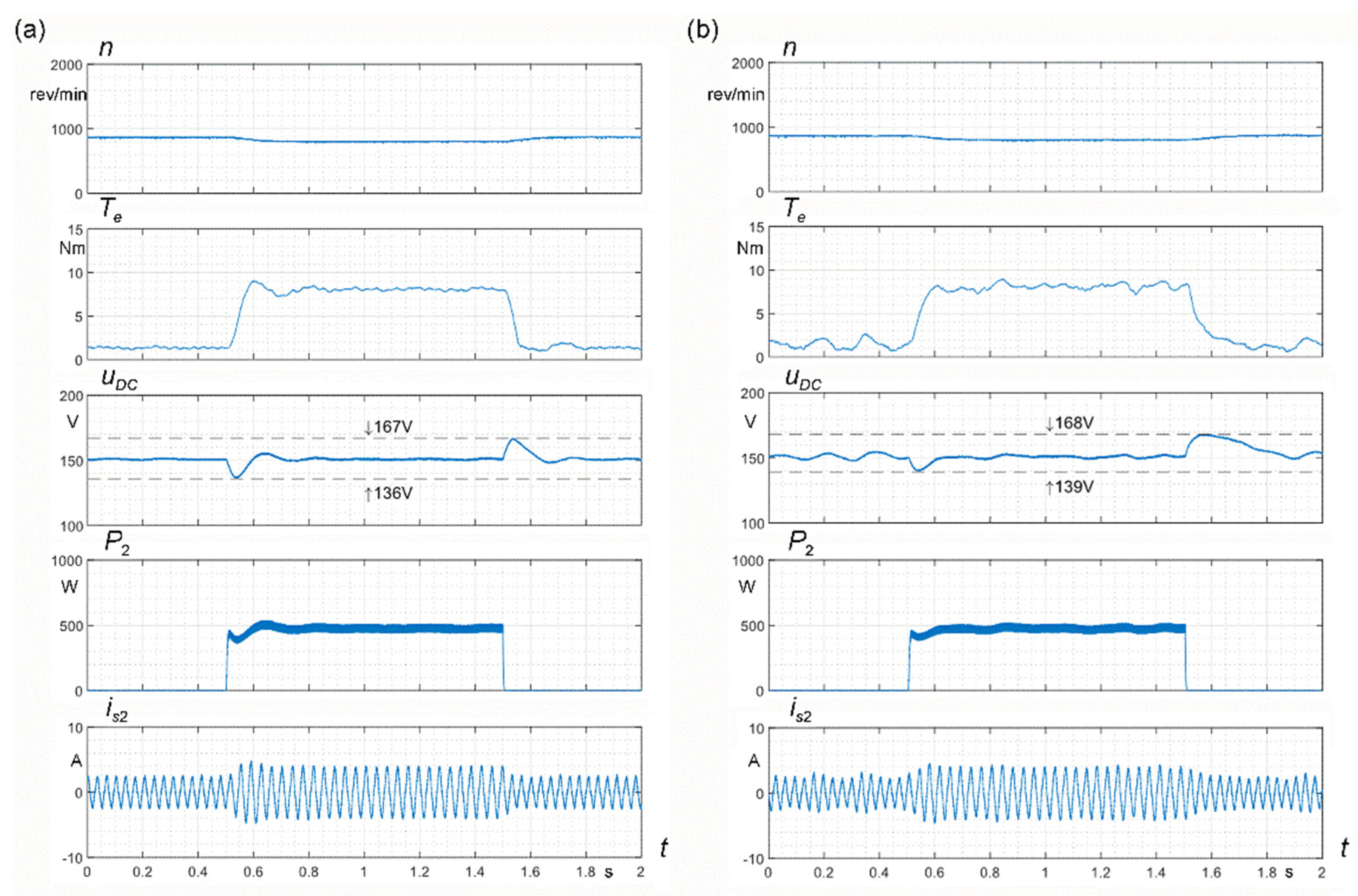
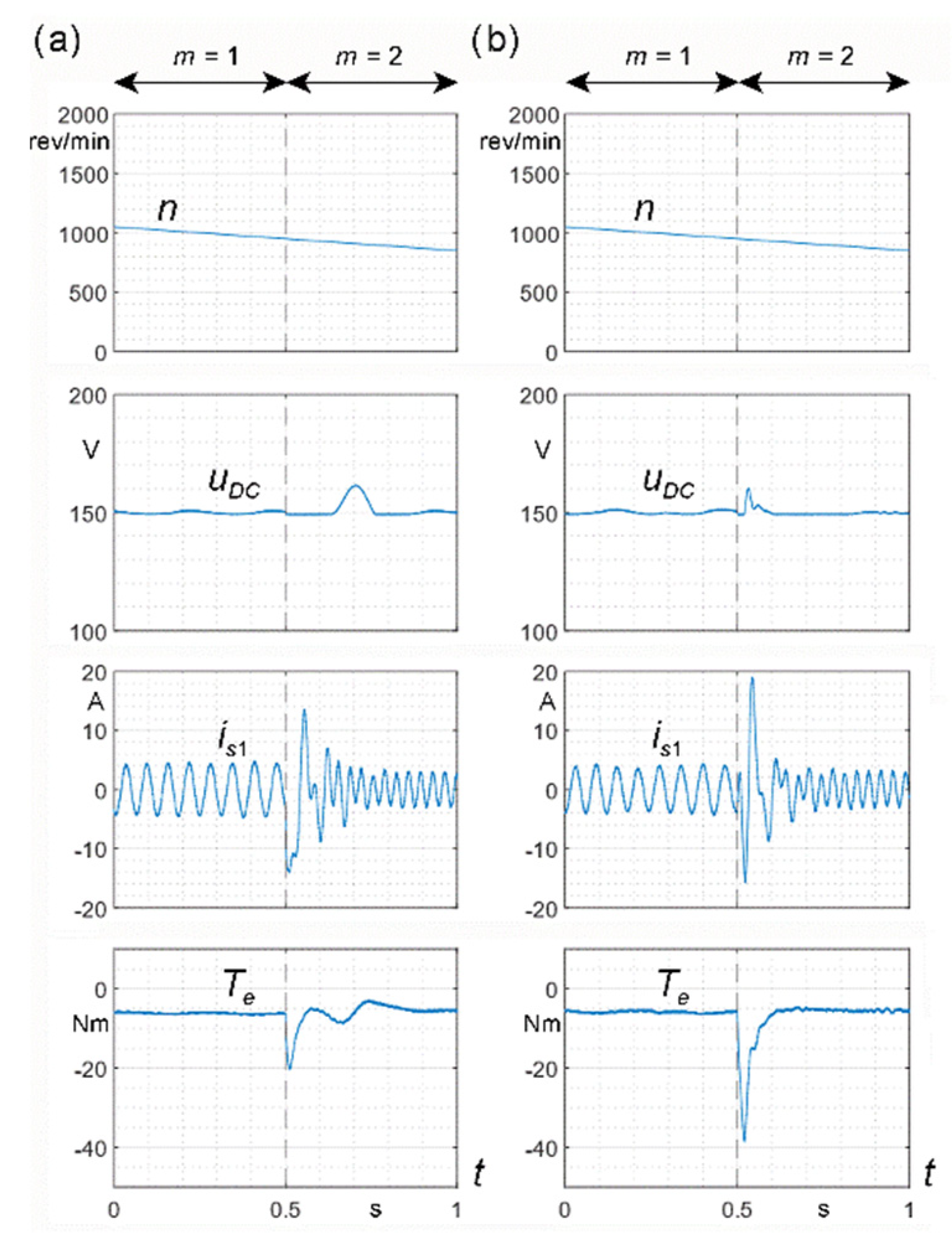
4.2. Results of Laboratory Tests

The tests of the generating system were carried out in the steady state for various power supply sequences and in transient states with a step change in the load and a change in the driving speed. The p. u. reference signal of the voltage controller was u D C r e f = 1.57 to keep the output voltage constant U D C = 150 V.

4.2.1. Steady-State Operation of the Generator

The steady-state operation of the generator was examined by setting its speed from ω p u = 0.2 to ω p u = 1.0 and measuring the driving torque T E , voltage u D C , stator current I s (rms), and load current i R d . The following values were determined: P 1 = T E n π 30 —mechanical input power, P 2 = R d I R d 2 —electrical output power, I d = P 2 / U D C —current supplying the DCSYS, η = P 2 / P 1 —energy conversion efficiency. The results of the measurements are presented in Figure 7 with the marked measurement points.
The regulation system maintained a constant voltage value at the output u D C = U D C = 150 V at all these points. Throughout the entire speed range and each sequence m, the stator current I s p u does not exceed the maximum output value I s y max p u = 1 of the voltage controller Ru, for which I s = I s N = 5.3 A. For example, we can explain the step change in the output power P 2 , shown in Figure 7, at the relative speed ω p u = 0.5. At this speed, m changes from 2 to 1 as the ω p u increases. The p. u. input power can be written as P 1 p u = T E p u ω p u . In the steady state, T E p u = T e p u . Assuming in (57), i s y p u I s p u , we obtain T E = m k Ψ p u ψ r p u I s p u . The rotor flux is kept as ψ r p u = 0.701 by the control system from Figure 5, whereas the stator current I s is controlled by Ru at a value such that u D C p u = u D C r e f = 1 ( u D C = 150 V). When ω p u is slightly lower than 0.5, the system operates at m = 2 . Then, k ψ ( m ) = 0.95 (Table 1), whereas the stator current read from Figure 7 is I s = 3.5 A. In p. u., it is I s p u = I s I s N = 3.5 5.3 = 0.66 , hence, T E p u ( m = 2 ) = 2 · 0.949 · 0.701 · 0.66 = 0.878 and P 1 p u ( m = 2 ) = 0.878 · 0.5 = 0.439 , giving P 1 ( m = 2 ) = P 1 p u ( m = 2 ) P o = 1413 W. When ω p u slightly increases over 0.5, parameter m changes to m = 1 . Then, the Ru forces the stator current to become the value I s p u = 1 to charge the capacitance C D C to the desired voltage as fast as possible, where the stator frequency changes from f s p u = 1 ( m = 2 ) to 0.5 ( m = 1 ). Parameter k ψ ( m ) = 0.986 (Table 1), ψ r p u = 0.701 , and T E p u ( m = 1 ) = 1 · 0.986 · 0.701 · 1.0 = 0.691 , P 1 p u ( m = 1 ) = 0.691 · 0.5 = 0.345 , giving P 1 ( m = 1 ) = P 1 p u ( m = 1 ) P o = 1110 W. The ratios k P c a l c u l a t e d = P 1 p u ( m = 2 ) P 1 p u ( m = 1 ) = 0.439 0.345 = 1.27 , k P m e a s u r e d = P 1 ( m = 2 ) P 1 ( m = 1 ) = 1250 1000 = 1.25 (Figure 7) are almost the same.
When m is switched from 2 to 1, the electrical power P 2 drops two times. The power P g crossing the air gap from the rotor to the stator is almost equal to P 1 , diminished with the power losses in the rotor winding Δ P r and in the magnetic core Δ P F e . The output power P 2 = P g ( 1 s ) can be written as P 2 = P g m ω p u , where the machine slip is s = 1 m ω Ω o = 1 m ω p u . Neglecting those power losses, we can write P 2 = P 1 m ω p u . So, at ω p u = 0.5 and m = 1 , the output power drops to P 2 1000 · 0.5 = 500 W , similarly for the point ω p u = 0.33 when m changes from 3 to 2. Hence, the generator efficiency is η m ω p u .
Figure 8 shows example waveforms corresponding to one point ω p u = 0.44, m = 2 of the characteristics from Figure 7. The waveforms for the other operating points are similar, and the main differences are in the shape of the phase voltage and current waveforms for given sequences m.

4.2.2. Dynamic Operation of the Generator

The minimum initial voltage U D C 0 (Figure 1) necessary to excite the generator was approximately 30 V. Figure 9 shows an example of the process of achieving the voltage U D C = 150 V of an unloaded generator operating with the sequence number m = 1 and the u D C r e f signal set linearly.
The step increase of the generator load is presented in the form of a comparison of the vector and scalar control in Figure 10. As can be seen, in both cases, the regulation system reacts similarly, although in the case of scalar control, larger oscillations of the regulated voltage appeared. In both cases, the voltage regulators had the same parameters. The regulators correct the voltage when the drive speed drops due to the load. The vector control can be improved by correcting the Ru parameters, e.g., increasing the signal of maximum current I s y max p u .
Switching the control sequence from m = 1 to m = 2 or m = 2 to m = 3 causes a torque surge T e of the generator, which affects the mechanical system. A comparison of such switching with vector and scalar control is shown in Figure 11. Switching from m = 1 to m = 2 occurs at a rotational speed of n = 1000 rev/min. Before switching ( m = 1), the generator operates at a frequency of approximately f s = 16.5 Hz, and after switching ( m = 2), the frequency increases almost twice. During switching, a negative electromagnetic torque surge T e occurs. It is twice as large with scalar control.
Additionally, it should be emphasized that the multiphase generator can produce the desired DC output voltage u D C while operating with broken phases of the stator or caused by VSC damage. This is illustrated in Figure 12 at decreasing speed and switching m when the first stator phase was broken. As one might expect, the difference between the symmetrical and asymmetrical work is negligible in this case. If more phases are broken, the generator still produces the set voltage, but the load power must be reduced. The waveforms in Figure 12 also show the correct response of the control system at a high variability of the generator speed.
To emphasize the advantages of a multiphase induction generator, its operation can be compared with a synchronous generator excited by permanent magnets (PMSG). The synchronous generator feeds a diode rectifier, the output of which is regulated by a back-boost converter at an appropriate value. At a reduced speed and a given load power, the multiphase induction generator operates at similar phase currents, while the synchronous generator must operate at much higher currents.

5. Conclusions

  • The field-oriented vector control of the multiphase squirrel-cage induction generator enables the proper regulation of the DC output voltage with changing load and speed. The generator speed depends on the driving system and its load. This is particularly visible in low-power wind turbines, for which this type of multiphase generator is dedicated. The advantage of this type of generator operating with sequence switching is that it produces a given voltage at low speeds with a greater efficiency than traditional SCCIG systems.
  • Multiphase machines may operate with damage to one or more phases [10,25]. The correct operation of the generator was demonstrated at speed variability and with asymmetry caused by the break of one phase.
  • The presented control method can be improved by the appropriate selection of voltage regulator parameters (gain, time constant, saturation), which can be achieved using computer simulation for the described mathematical model.
  • Scalar control does not require the same signal processing as vector control. It causes slightly worse control properties, manifested as larger torque surges when switching the control sequence. The system is simpler, more reliable, and can be modified to some degree. The quality of regulation was comparable to the vector control since in both control systems, the same voltage regulator was used. However, the vector control has a lot more possibilities of modifications.
  • The presented method of controlling the nine-phase generator can be used to control squirrel-cage induction generators with a different number of phases, e.g., M = 5, M = 7, M = 15. One should be aware that the control system is based on a simplified mathematical model assuming only one harmonic of the order ν / = m associated with the control sequence m . In fact, there is also the influence of higher harmonics, shown in the presented mathematical model, especially of the order ν / = | m ± M | .
  • Based on the presented results, it can be concluded that multiphase generators of this type are suitable for low-power wind turbines, because by controlling the change in m , a mechanical gearbox can be eliminated.
  • To further improve the control performance, other advanced techniques could be applied [26,27,28,29].
  • The presented research was carried out as part of a doctoral dissertation [30]. The mathematical model can be adopted for the description of the multiphase induction machines with numbers of phases other than 9 and can be used to analyze the motor and generator operation.

Author Contributions

Conceptualization, D.C. and P.D.; Methodology, D.C. and P.D.; Validation, D.C. and P.D.; Formal analysis, D.C. and P.D.; Investigation, D.C. and P.D.; Resources, D.C. and P.D.; Data curation, D.C. and P.D.; Writing—original draft, P.D.; Writing—review & editing, D.C. and P.D.; Visualization, D.C. and P.D.; Supervision, P.D. All authors have read and agreed to the published version of the manuscript.

Funding

Ministry of Science and Higher Education: Subsidies on science granted for Cracow University of Technology.

Data Availability Statement

Dataset available on request from the authors.

Conflicts of Interest

The authors declare no conflict of interest.

References

  1. Drozdowski, P.; Cholewa, D. Voltage Control of Multiphase Cage Induction Generators at a Speed Varying over a Wide Range. Energies 2021, 14, 7080. [Google Scholar] [CrossRef]
  2. Boldea, I. Variable Speed Generators (Electric Power Engineering Series); CRC, Taylor&Francis Group: Boca Raton, FL, USA, 2005; ISBN/ASIN: 0849357152. [Google Scholar]
  3. Domínguez-García, J.L.; Gomis-Bellmunt, O.; Trilla-Romeroa, L.; Junyent-Ferré, A. Indirect vector control of a squirrel cage induction generator wind turbine. Comput. Math. Appl. 2012, 64, 102–114. [Google Scholar] [CrossRef]
  4. Kumsuwan, Y.; Srirattanawichaikul, W.; Premrudeepreechacharn, S. A Simple Voltage and Frequency Control of VSI-Inverter-Fed Self-Excited Induction Generator Drive. In Proceedings of the ICROS-SICE International Joint Conference, Fukuoka, Japan, 18–21 August 2009; pp. 430–434. [Google Scholar]
  5. Peng, X.; Liu, Z.; Jiang, D. A review of multiphase energy conversion in wind power generation. Renew. Sustain. Energy Rev. 2021, 147, 111172. [Google Scholar] [CrossRef]
  6. Chen, Z.; Guerrero, J.M.; Blaabjerg, F. A Review of the State of the Art of Power Electronics for Wind Turbines. IEEE Trans. Power Electron. 2009, 24, 1859–1875. [Google Scholar] [CrossRef]
  7. Baroudi, J.A.; Dinavahi, V.; Knight, A.M. A review of power converter topologies for wind generators. Renew. Energy 2007, 32, 2369–2385. [Google Scholar] [CrossRef]
  8. Chinmaya, K.A.; Singh, G.K. Modeling and experimental analysis of grid-connected six-phase induction generator for variable speed wind energy conversion system. Electr. Power Syst. Res. 2019, 166, 151–162. [Google Scholar] [CrossRef]
  9. Kali, Y.; Saad, M.; Rodas, J.; Mougharbel, I.; Benjelloun, K. Robust Control of a 6-Phase Induction Generator for Variable Speed Wind Energy Conversion System. In Proceedings of the 2020 5th International Conference on Renewable Energies for Developing Countries (REDEC), Marrakech, Morocco, 29–30 June 2020; IEEE: Piscataway, NJ, USA, 2020. [Google Scholar]
  10. Pantea, A.; Yazidi, A.; Betin, F.; Carrière, S.; Sivert, A.; Vacossin, B.; Henao, H.; Capolino, G.-A. Fault-tolerant control of a low-speed six-phase induction generator for wind turbine. IEEE Trans. Ind. Appl. 2019, 55, 426–436. [Google Scholar] [CrossRef]
  11. Jakubowski, B.; Pieńkowski, K. Analysis and synthesis of converter control system of autonomous induction generator with field oriented control. Arch. Electr. Eng. 2013, 62, 267–279. [Google Scholar] [CrossRef]
  12. Mihet-Popa, L.; Boldea, I. Variable Speed Wind Turbines using Induction Generators Connected to the Grid: Digital Simulation versus Test Results. In Proceedings of the IEEE—The 9th International Conference on Optimization of Electrical and Electronic Equipment, OPTIM 2004, Braşov, Romania, 20–21 May 2004. 8p. [Google Scholar]
  13. Beainy, A.; Maatouk, C.; Moubayed, N.; Kaddah, F. Comparison of Different Types of Generator for Wind Energy Conversion System Topologies. In Proceedings of the 2016 3rd International Conference on Renewable Energies for Developing Countries (REDEC), Zouk Mosbeh, Lebanon, 13–15 July 2016. [Google Scholar]
  14. Sibanda, A.; Gule, N. Modelling of a Grid Connected Nine-Phase Induction Generator. In Proceedings of the 2020 International Symposium on Power Electronics, Electrical Drives, Automation and Motion, Sorrento, Italy, 24–26 June 2020; IEEE: Piscataway, NJ, USA, 2020; pp. 799–804. [Google Scholar]
  15. Amimeur, H.; Aouzellag, D.; Abdessemed, R.; Ghedamsi, K. Sliding mode control of a dual-stator induction generator for wind energy conversion systems. Int. J. Electr. Power Energy Syst. 2012, 42, 60–70. [Google Scholar] [CrossRef]
  16. Muljadi, E.; Butterfield, C.P.; Handman, D. Dual-Speed Wind Turbine Generation; National Renewable Energy Laboratory: Golden, CO, USA, 1996.
  17. Talpone, J.I.; Puleston, P.F.; Cendoya, M.G.; Barrado-Rodrigo, K.A.A. Dual-Stator Winding Induction Generator Based Wind-Turbine Controlled via Super-Twisting Sliding Mode. Energies 2019, 12, 4478. [Google Scholar] [CrossRef]
  18. Maciejewski, P.; Iwański, G. Six-phase doubly fed induction machine-based standalone DC voltage generator. Bull. Pol. Acad. Sci. 2021, 69, e135839. [Google Scholar] [CrossRef]
  19. Mengjie, L.; Lingxiang, W.; Zhen, X. Control strategy of wide-speed-range doubly fed induction generator, based on stator winding short circuited in low speed mode. In Proceedings of the 36th Chinese Control Conference (CCC), Dalian, China, 26–28 July 2017. [Google Scholar]
  20. Yaramasu, V.; Wu, B.; Sen, P.C.; Kouro, S.; Narimani, M. High-Power Wind Energy Conversion Systems: State-of-the-Art and Emerging Technologies. Proc. IEEE 2015, 103, 740–788. [Google Scholar] [CrossRef]
  21. Thongam, J.S.; Bouchard, P.; Ezzaidi, H.; Ouhrouche, M. Wind Speed Sensorless Maximum Power Point Tracking Control of Variable Speed Wind Energy Conversion Systems. In Proceedings of the 2009 IEEE International Electric Machines and Drives Conference, Miami, FL, USA, 3–6 May 2009; pp. 1832–1837. [Google Scholar]
  22. Ciupageanu, D.A.; Gheorghe, L.G.; Barelli, L. Wind energy integration: Variability analysis and power system impact assessment. Energy 2019, 185, 1183–1196. [Google Scholar] [CrossRef]
  23. Drozdowski, P. Speed control of multiphase cage induction motors incorporating supply sequence. Arch. Electr. Eng. 2014, 63, 511–534. [Google Scholar] [CrossRef]
  24. Drozdowski, P. The universal mathematical model for multiphase cage induction motors. Electr. Mach. KOMEL Trans. 2015, 3, 19–24. [Google Scholar]
  25. Gonzalez Prieto, I.; Duran, M.J.; Garcia-Entrambasaguas, P.; Bermude, M. Field-Oriented Control of Multiphase Drives with Passive Fault Tolerance. IEEE Trans. Ind. Electron. 2020, 67, 7228–7723. [Google Scholar] [CrossRef]
  26. Carrillo-Rios, J.; Gonzalez-Prieto, I.; Gonzalez-Prieto, A.; Duran, M.J.; Aciego, J.J. Long-Prediction Horizon FCS-MPC for Multiphase Electric Drives with a Selective Control Action Promotion. IEEE Trans. Ind. Electron. 2023, 1–12. [Google Scholar] [CrossRef]
  27. Lim, S.C.; Lee, S.S.; Levi, E. Continuous-Control-Set Model Predictive Current Control of Asymmetrical Six-Phase Drives Considering System Nonidealities. IEEE Trans. Ind. Electron. 2023, 70, 7615–7626. [Google Scholar] [CrossRef]
  28. Martın, C.; Arahal, M.R.; Barrero, F.; Duran, M.J.; Gonzalez-Prieto, I. Variable Sampling Time Model Predictive Control of Multiphase Induction Machines. In Proceedings of the 2018 IEEE 15th International Workshop on Advanced Motion Control (AMC), Tokyo, Japan, 9–11 March 2018. [Google Scholar]
  29. Levi, E. Advances in Converter Control and Innovative Exploitation of Additional Degrees of Freedom for Multiphase Machines. IEEE Trans. Ind. Electron. 2016, 63, 433–448. [Google Scholar] [CrossRef]
  30. Cholewa, D. Analysis and Control of Multiphase Cage Induction Generators. Ph.D. Thesis, Cracow University of Technology, Kraków, Poland, 2023. (In Polish). [Google Scholar]
Figure 1. General structure of the automatic DC voltage control and the connection system: MIM—multiphase induction machine, VSC—voltage source converter, GE—generator engine (e.g., a wind or water turbine), GB—gear box (optional), CM—phase current measurement, UDC0—system assuring a minimum voltage of CDC, DB—blocking diode, DCSYS—single resistance load (the simplest) or power grid supplied with the grid side converter, CTRL—control system, T—speed sensor (e.g., tachometric generator, pulse encoder), ωpu—speed signal of the MIM related to the base reference speed Ωo, uDCref—DC bus voltage control signal.
Energies 17 00790 g001
Figure 2. Arrangement of the nine-phase winding with p = 1 (α = 10°, β = 60°); beginnings of the phase windings: 1, 2, 3…, 9 endings of the phase windings: 1′, 2′, 3′,…, 9′.
Energies 17 00790 g002
Figure 3. Illustration of mechanical characteristics of the nine-phase induction generator driven with the wind turbine.
Energies 17 00790 g003
Figure 4. Vector diagram for field-oriented control of the multiphase generator.
Energies 17 00790 g004
Figure 5. Control scheme of the generator.
Energies 17 00790 g005
Figure 6. Rotor flux vector estimator EST (current model of rotor flux).
Energies 17 00790 g006
Figure 7. Steady-state characteristics of the nine-phase induction generator versus the speed ωpu of the range 0.2 … 1.0.
Energies 17 00790 g007
Figure 8. Waveforms illustrating the generator operation at speed ωpu = 0.44 and supply sequence m = 2.
Energies 17 00790 g008
Figure 9. Controlled exciting process of the no-load generator operating at m = 1 and ωpu = 0.7 (1400 rev/min).
Energies 17 00790 g009
Figure 10. Response to a sudden increase in the load of the generator: (a) vector control, (b) scalar control.
Energies 17 00790 g010
Figure 11. Effect of switching the control sequence from m = 1 to m = 2: (a) vector control, (b) scalar control.
Energies 17 00790 g011
Figure 12. Vector-controlled nine-phase generator operating with one phase broken during varying speed.
Energies 17 00790 g012
Table 1. Mathematical model parameters for the control system.
ParameterUnitm = 1m = 2m = 3m = 4
L μ ( m ) H0.2820.2070.1180.047
L μ ( m ) p u 4.6333.4011.9380.772
L s ( m ) H0.3170.2380.1450.084
L s ( m ) p u 5.2073.9092.3821.38
L r ( m ) H0.2860.2180.1380.058
L r ( m ) p u 4.6983.5812.2670.953
R s Ω1.31.31.31.3
R s p u 0.1020.1020.1020.102
R r ( m ) Ω0.4580.9491.1440.811
R r ( m ) p u 0.0360.0740.090.064
T r ( m ) s0.6240.2300.1200.071
L a ( m ) H0.040.0410.0440.046
L a ( m ) p u 0.640.680.720.75
k Ψ ( m ) 0.9860.9490.8550.810
R a ( m ) Ω1.7452.1552.1361.832
R a ( m ) p u 0.1370.1690.1670.144
T a ( m ) s0.02230.01920.02060.0250
Disclaimer/Publisher’s Note: The statements, opinions and data contained in all publications are solely those of the individual author(s) and contributor(s) and not of MDPI and/or the editor(s). MDPI and/or the editor(s) disclaim responsibility for any injury to people or property resulting from any ideas, methods, instructions or products referred to in the content.

