Article

An Artificial Neural Network-Based Fault Diagnostics Approach for Hydrogen-Fueled Micro Gas Turbines †

by
Muhammad Baqir Hashmi
1,*,
Mohammad Mansouri
1,2,
Amare Desalegn Fentaye
3,
Shazaib Ahsan
4 and
Konstantinos Kyprianidis
3
1
Department of Energy and Petroleum Engineering, University of Stavanger, 4036 Stavanger, Norway
2
NORCE Norwegian Research Centre, 4021 Stavanger, Norway
3
School of Business, Society and Engineering, Mälardalen University, P.O. Box 883, SE-721 23 Västerås, Sweden
4
Department of Mechanical Engineering, University of Manitoba, Winnipeg, MB R3T 5V6, Canada
*
Author to whom correspondence should be addressed.
This article is the extended version of the paper published in Proceedings of the 64th International Conference of Scandinavian Simulation Society, SIMS 2023 Västerås, Sweden, 25–28 September 2023.
Energies 2024, 17(3), 719; https://doi.org/10.3390/en17030719
Submission received: 28 December 2023 / Revised: 24 January 2024 / Accepted: 31 January 2024 / Published: 2 February 2024
(This article belongs to the Section A: Sustainable Energy)

Abstract

:
The utilization of hydrogen fuel in gas turbines brings significant changes to the thermophysical properties of flue gas, including higher specific heat capacities and an enhanced steam content. Therefore, hydrogen-fueled gas turbines are susceptible to health degradation in the form of steam-induced corrosion and erosion in the hot gas path. In this context, the fault diagnosis of hydrogen-fueled gas turbines becomes indispensable. To the authors’ knowledge, there is a scarcity of fault diagnosis studies for retrofitted gas turbines considering hydrogen as a potential fuel. The present study, however, develops an artificial neural network (ANN)-based fault diagnosis model using the MATLAB environment. Prior to the fault detection, isolation, and identification modules, physics-based performance data of a 100 kW micro gas turbine (MGT) were synthesized using the GasTurb tool. An ANN-based classification algorithm showed a 96.2% classification accuracy for the fault detection and isolation. Moreover, the feedforward neural network-based regression algorithm showed quite good training, testing, and validation accuracies in terms of the root mean square error (RMSE). The study revealed that the presence of hydrogen-induced corrosion faults (both as a single corrosion fault or as simultaneous fouling and corrosion) led to false alarms, thereby prompting other incorrect faults during the fault detection and isolation modules. Additionally, the performance of the fault identification module for the hydrogen fuel scenario was found to be marginally lower than that of the natural gas case due to assumption of small magnitudes of faults arising from hydrogen-induced corrosion.

1. Introduction

The heat and power sector was responsible for ~38% of global carbon dioxide emissions in 2021. Natural gas (NG) reportedly contributed to ~22% of the electric power generation globally in 2021 [1]. By far, gas turbines are mainly burning NG for power generation, resulting in greenhouse gas (GHG) emissions and climate change. Therefore, the decarbonization of gas turbines becomes indispensable to meet the global energy transition mandate. In this context, the gas turbine industry is aiming for 100% carbon-neutral gas-fired power generation using low-carbon fuels, such as hydrogen, by 2030 [2].
Nevertheless, the utilization of hydrogen in gas turbines raises several technological and reliability challenges due to the different thermophysical properties of hydrogen as compared to NG. For instance, hydrogen can potentially lead to flashback and thermoacoustic instabilities in the lean premixed dry low-emissions/dry low-NOx (DLE/DLN) burners. Flashback can damage the upstream components of the burner. It is worth noticing that available DLN technologies are currently capable of burning up to 60% hydrogen [3], with a few exceptions, such as the recent firing of the Siemens SGT-400 with 100% hydrogen for limited operational hours [4]. The utilization of 100% hydrogen requires the reconfiguration of the gas turbine with a new hydrogen-compliant burner and a modified fuel system. Even then, high hydrogen utilization produces an enhanced steam content in the combustion flue gas that, in turn, is responsible for high heat transfer to the metal parts, higher thermal conductivity, aggravated oxidation corrosion, increased creep, and thermal fatigue damage to the hot-gas-path components [5]. Consequently, hydrogen-fueled gas turbines are susceptible to more health degradation caused by the already-mentioned problems. Especially, the retrofitted gas turbines, in which solely the burner is replaced with a hydrogen-compliant burner and the existing turbomachinery is kept, have a greater propensity for health degradation. Therefore, advanced intelligent fault diagnosis, prognosis, and health monitoring are of crucial importance for the enhanced reliability and availability of hydrogen-fueled gas turbines.
Normally, as the operating hours of gas turbines increase, the performance and health degrade due to various component faults [6]. To carry out effective maintenance actions, timely fault detection and identification play a key role in assuring the reliability of the engines. Fault diagnosis has been performed over the years for industrial and aerogas turbines. It started with Urban’s rudimentary concept of linear gas-path analysis (GPA) [7,8]. Nowadays, gas turbine gas-path diagnostics are typically carried out via model-based, data-driven, and hybrid approaches [9]. To gain more accuracy in the fault diagnostics, digital twins have also been suggested in the most recent literature. For instance, the digital twin developed by Hu et al. [10] showed a fault diagnostic error between the actual and predicted values on the order of ±2% that was reportedly promising. A variety of studies exist in the literature pertinent to component degradation, fault detection, and the diagnosis of both industrial and aero-derivative gas turbines [11,12,13,14], and a short summary focusing on the studies during the past five years is listed in Table 1.
For micro gas turbines, there are a few studies relevant to performance-based fault diagnosis that considered radial compressor fouling, turbine erosion, and recuperator degradation phenomena, all considering NG-fueled scenarios. Gomes et al. [27] reported that the presence of the recuperator in the MGT increases the sensitivity of the engine to compressor fouling and turbine erosion, especially in the variable-speed operating mode. They conducted a comparative study of several single and multiple faults, including fouling, erosion, foreign object damage (FOD), and recuperator deterioration. The study adopted a model-based approach, namely, the nonlinear GPA (NLGPA) technique, using Pythia and Turbomatch tools for the fault diagnosis. Another study conducted by Yoon et al. [28] employed neural networks for the prediction of the degraded performance of 30 kW MGT. Various kinds of single and multiple faults in the compressor, turbine, and recuperator were included in the study. The approach was found to be predicting the results with much accuracy, even if some of the measurement data were missing.
Talebi and Tousi [29] attributed compressor fouling as one of the majorly occurring faults in the MGT engine; hence, they investigated the effect of blade surface roughness on the performance degradation of radial turbomachinery in a 477 kW MGT. The study revealed that the combustor inlet temperature and turbine outlet temperature were more sensitive to blade surface roughness because these measurements showed values greater than the allowable limits. However, the compressor discharge temperature was found to be less sensitive to the roughness. In a similar study, Bauwens [30] also asserted that compressor fouling was a highly likely occurring fault in a 3 kW MTT MGT because of the possibility of oil ingestion in the compressor originating from a deaerating oil sump. A recent study conducted by Hashmi et al. [31] reported the effect of steam-induced corrosion on the performance degradation of a hydrogen-fueled MGT. The amount of steam was found to be more than twice (mass fraction of H2O with NG: 0.1239; mass fraction of H2O with H2: 0.2548) than that of a natural gas combustion scenario. Talebi et al. [32] utilized an artificial neural network (ANN) for the fault detection and isolation of a 100 kW MGT considering the measurement uncertainties at different part-load settings. The main faults considered in their study were the compressor, turbine, and recuperator.
Diving deep into the literature manifests that gas turbines running on 100% hydrogen fuel are susceptible to increased hydrogen-induced corrosion due to the different thermophysical properties and the enhanced steam content of the hydrogen fuel as compared to the NG fuel. The compressor is also highly vulnerable to fouling when the gas turbine’s operating hours are increased. The gas turbine industry has recently tested their gas turbines with 100% hydrogen for limited operating hours. However, gas turbines would most likely be exposed to longer operating hours with hydrogen fuel in the future. That would affect their health and performance, and the industry has a critical need to seek solutions for hydrogen-related faults. In addition, the existing gas turbines are currently being retrofitted with new hydrogen-compliant burners. Solely in the retrofitted gas turbines, the burner is replaced with a new burner, while the rest of the components, i.e., the turbomachinery components, are not changed. This kind of retrofitting exposes the hot-gas-path components, especially the turbine, to enhanced steam, in the case of hydrogen fuel, that can potentially cause enhanced corrosion as compared to the NG case.
In line with industry ambitions towards energy transition, a 100 kW MGT test facility at the University of Stavanger was recently retrofitted with a FLOX burner capable of burning 100% hydrogen [33]. The existing turbomachinery components from the OEM were retained. In this regard, it was imperative to investigate the effect of various hydrogen-induced faults and their timely diagnosis to ensure an increased reliability and availability. However, an in-depth literature search revealed that hydrogen-induced corrosion in the hot-gas-path components of both larger gas turbines and MGTs had not been investigated before based on the authors’ best knowledge. These research gaps paved the way for the development of a fault detection, isolation, and identification model for a 100 kW MGT running with pure hydrogen fuel.
The present study incorporates a thermodynamic model using the commercial tool GasTurb 14 [34] to generate validated design-point and off-design performance data. Data preprocessing was implicated to add noise and correct the data for ambient condition variations. Subsequently, the data were fed into classification and regression learner tools in MATLAB (release 2022a) for fault detection and diagnosis purposes using a neural network approach.

2. Methodology

The overall methodology of the entire study consists of 7 steps. The workflow includes developing a physics-based performance model, validating the model with real-time MGT data, implanting the physical faults using health parameters, i.e., the flow capacity and efficiency, the processing of the synthesized performance data, fault detection and isolation (FDI), fault identification, and, finally, the testing and validation of the algorithms. Data processing is further segregated into correcting the data against ambient conditions, finding the measurement deltas of the signals, and the noise addition. Subsequently, the corrected–measured–noisy data of the signals are fed to ANN-based classification and regression algorithms to develop a holistic fault diagnosis model. The different steps of the fault diagnosis process are illustrated in Figure 1. The details of these steps are described in the following subsections.

2.1. Baseline Performance Model

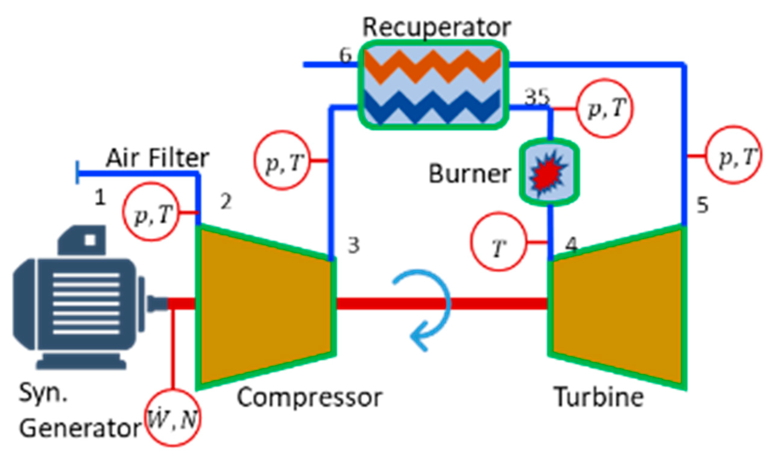
A thermodynamic performance model of a 100 kW MGT was initially developed using the commercial software tool GasTurb 14 [34] for physics-based data generation. The schematic of the MGT with sensor measurement points at various gas-path stations is illustrated in Figure 2.
The station numbers have been identified at their respective positions. For instance, 2 is labeled as the compressor intake, 3 as the compressor exhaust, 35 as the recuperator cold-side exhaust, 4 as the turbine inlet, 5 as the turbine exhaust, and 6 as the recuperator hot-side exhaust. The design-point calculations were optimized using a random search algorithm to ensure the accuracy of the baseline model. The off-design performance was calibrated with the experimental data for accurate validation purposes. The experiments were conducted at different power settings, varying from 50 to 100 kW, with a step change of 10 kW. The ambient temperatures were noticed to vary between 281.15 and 287.15 K during the entire test campaign. The real-time data were obtained by installing different pressure and temperature sensors in the form of probes. To measure the gas-path conditions at the intake of the compressor, five pressure- and four temperature-measuring sensors were installed. Similarly, at the compressor exit, three pressure- and three temperature-measuring sensors were installed 120° apart at circumferential positions to measure the average values at the flow field. Additionally, the combustor head was also encompassed with pressure and temperature sensors to measure the conditions of the intake air preheated by the recuperator. The instruments used for measuring the pressure at different points were Kiel probes installed ±35° apart. Pressure scanners were adopted to scan the pressure with an accuracy of 0.05 for full-scale output. Similarly, for the temperature measurements, K-type thermocouples with an accuracy of ±1 K were installed, and a data acquisition (DAQ) device was utilized to obtain the measured data. Subsequently, the pressure scanner and the DAQ were connected to a computer in parallel mode via two ports, which led to data visualization with the LabView software. The validated design-point data are listed in Table 2.
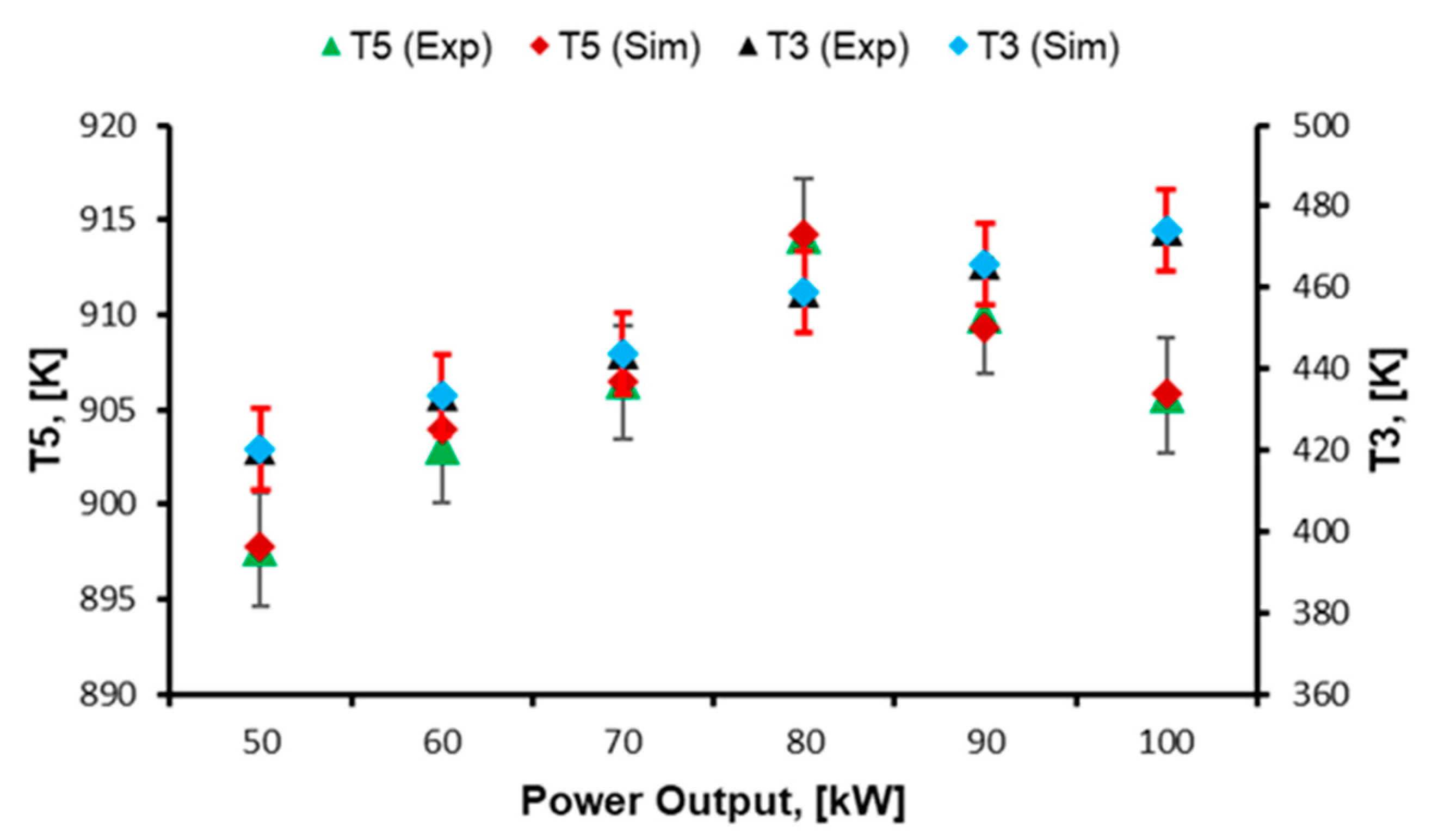
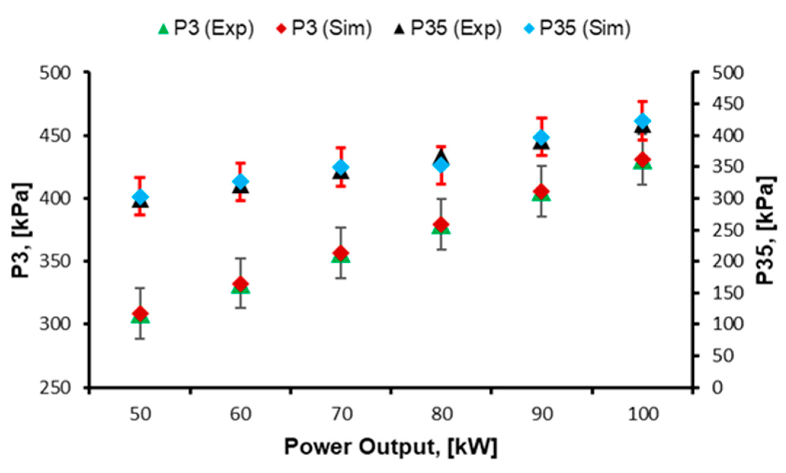
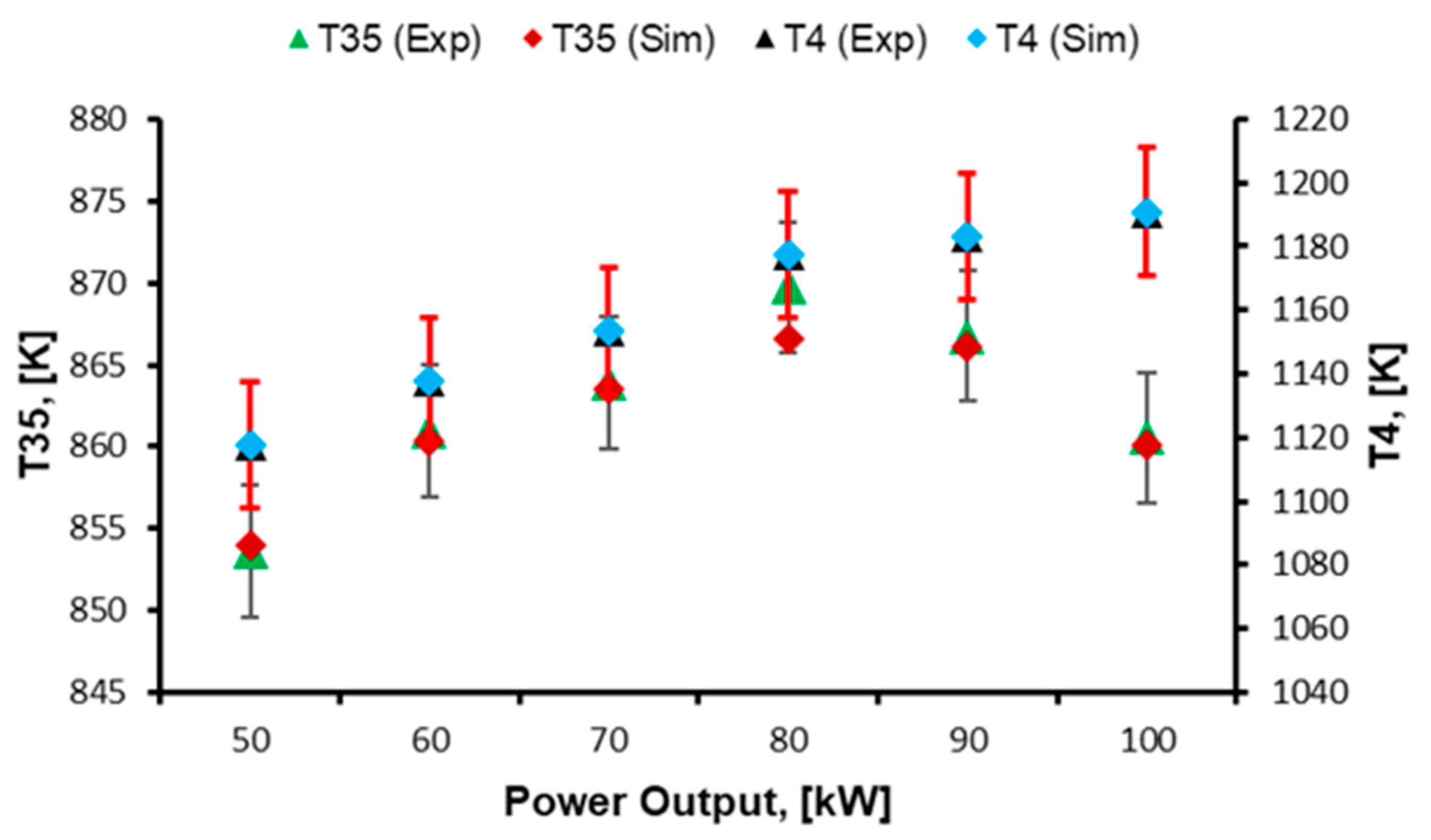
The validated off-design data at different part-load power settings for different measurement points are illustrated in Figure 3, Figure 4, Figure 5 and Figure 6. Firstly, the engine was simulated by assuming NG as a working fuel that basically established a baseline for further model development. Subsequently, the hydrogen was utilized as a fuel that was the prime objective of the study. Both simulation scenarios, i.e., the use of NG and hydrogen, were further went through noise addition to mimic the measurement uncertainties along with the ambient temperature corrections. These data were further normalized to generate residuals between the healthy and degraded engine conditions. Finally, these data were made ready for classification and regression learning by employing an artificial neural network to carry out the fault detection, isolation, and identification. Based on the deviating fault signatures, the measurement signals of P3, T3, P35, T35, T4, and T5 were identified as the most significant parameters for fault diagnosis purposes.

2.2. Component-Level Degradation

The physical faults, such as fouling, corrosion, erosion, and FOD, occurring in different components of the gas turbine systems lead to variations in the engine health parameters or independent parameters, i.e., the flow capacity and isentropic efficiencies. These health parameters, in turn, stimulate deviations in the engine measurements or dependent parameters, such as the pressure, temperature, fuel flow, and shaft speed. The present study employed the nonlinear GPA (NLGPA) approach for the gas-path diagnostics of the MGT because of its added advantage over the LGPA in terms of accuracy [9]. This is a model-based diagnosis approach that employs a thermodynamic relationship between dependent and independent parameters, addressing the nonlinearity of the gas turbine engine. The correlations are as follows,
Z = H . X
Z is a vector of the measurement deviations of a degraded engine condition from a clean condition. The clean condition is normally assumed as the healthy condition of the engine at the design point. X expresses the health parameters and H represents the influence of the coefficient matrix (ICM) that develops a correlation between Z and X . Further details can be found in the existing literature, such as [9,36].
The current study encompassed two kinds of component faults, i.e., compressor fouling and turbine corrosion. The reason for choosing fouling was mainly due to its high probability of occurrence in recuperated MGTs, as evidenced by the literature [27,30]. Turbine corrosion was selected because hydrogen fuel leads to an enhanced steam content that can cause higher heat transfer rates and corrosion as compared to an NG-fueled gas turbine [37]. These H2-specific attributes can further lead to aggravated creep and material degradation in the hot-gas-path components, and hence to the reduced lifetime of the gas turbine. The quantification of the components’ physical faults was carried out by developing the scaling factors of the health parameters (flow capacity: Γ ; efficiency: η ), as follows,
Γ d e g = Γ c l e a n ( 1 + Δ Γ / 100 )
η d e g = η c l e a n ( 1 + Δ η / 100 )
In the abovementioned equations, the subscript “ d e g ” represents the degraded component condition, while “ c l e a n ” represents the engine’s clean or healthy condition; Δ denotes the change in the health parameters. To develop fault diagnosis models for gas turbines, a variety of fault magnitudes have been assumed by the literature that show a relative change in the flow capacity and the isentropic efficiency from the clean condition in the form of scaling or correction factors. Table 3 lists the values of the compressor and turbine degradation magnitudes with their respective ratios. It is worth mentioning that the fault magnitude of the fouling has been assumed to be similar for both fuel scenarios, while the fault magnitude of the turbine corrosion for the hydrogen fuel has been assumed to be higher than that of NG. The assumption for steam-induced corrosion has been borrowed from a study by Zwebek and Pilidis [38,39] that was conducted for the fault diagnosis of the steam turbine. The reason lies in the fact that propagation mechanism of steam-induced corrosion behaves similarly in both steam and gas turbines, though it is caused by hydrogen fuel usage in the latter type.

2.3. Fault Diagnosis

The diagnosis of the gas turbines is normally performed in three steps, i.e., fault detection, fault isolation, and, finally, fault identification. Fault detection provides information about the presence of any imminent physical abnormality in the system. Fault isolation helps in determining the exact type and location of the fault. Fault identification determines the severity magnitude of the any physical fault. The present study incorporated all these steps involved in the diagnosis, as shown in Figure 1.

2.3.1. Data Processing

Prior to the fault diagnosis of the MGT, the data generated from the performance model went through a preprocessing phase. During preprocessing, the data were first segregated on a fuel basis, i.e., NG and hydrogen. Subsequently, a fault-wise segregation (i.e., compressor fouling, turbine corrosion, and simultaneous compressor fouling and turbine corrosion) was carried out. Temperature corrections were also performed to avoid the influence of the ambient temperature variations on the measurement signals, as follows,
  θ = T m e a s u r e d 288.15   K  
where θ is the correction factor of the measured temperature ( T m e a s u r e d ) with respect to the design ambient temperature of 288.15 K.
Measurement deviations of the degraded conditions from the clean condition of each signal, i.e., P3, T3, P35, T35, T4, T5, and P5, were estimated using the following equation,
Δ Z = ( Z d e g Z c l e a n ) Z c l e a n × 100
where Δ Z is the measurement deviation vector between the healthy/clean engine sensor data ( Z c l e a n ) and the degraded engine data ( Z d e g ). Furthermore, noise was added to the measurement deltas to account for measurement uncertainties that could happen in the experimental data. The standard deviation for the Gaussian distribution was assumed to be 1% for the temperature signals, while it was assumed to be 0.5% for the pressure signals. The equation involved in the noise generation using the random function was as follows,
x = 1 + 2 × r a n d ( 1 , N )
where N expresses the number of sample points including clean and faulty engine data. A total of 800 sample points were generated, i.e., 400 samples for each of the NG and hydrogen fuel scenarios.

2.3.2. ANN-Based Classification (Fault Detection and Isolation)

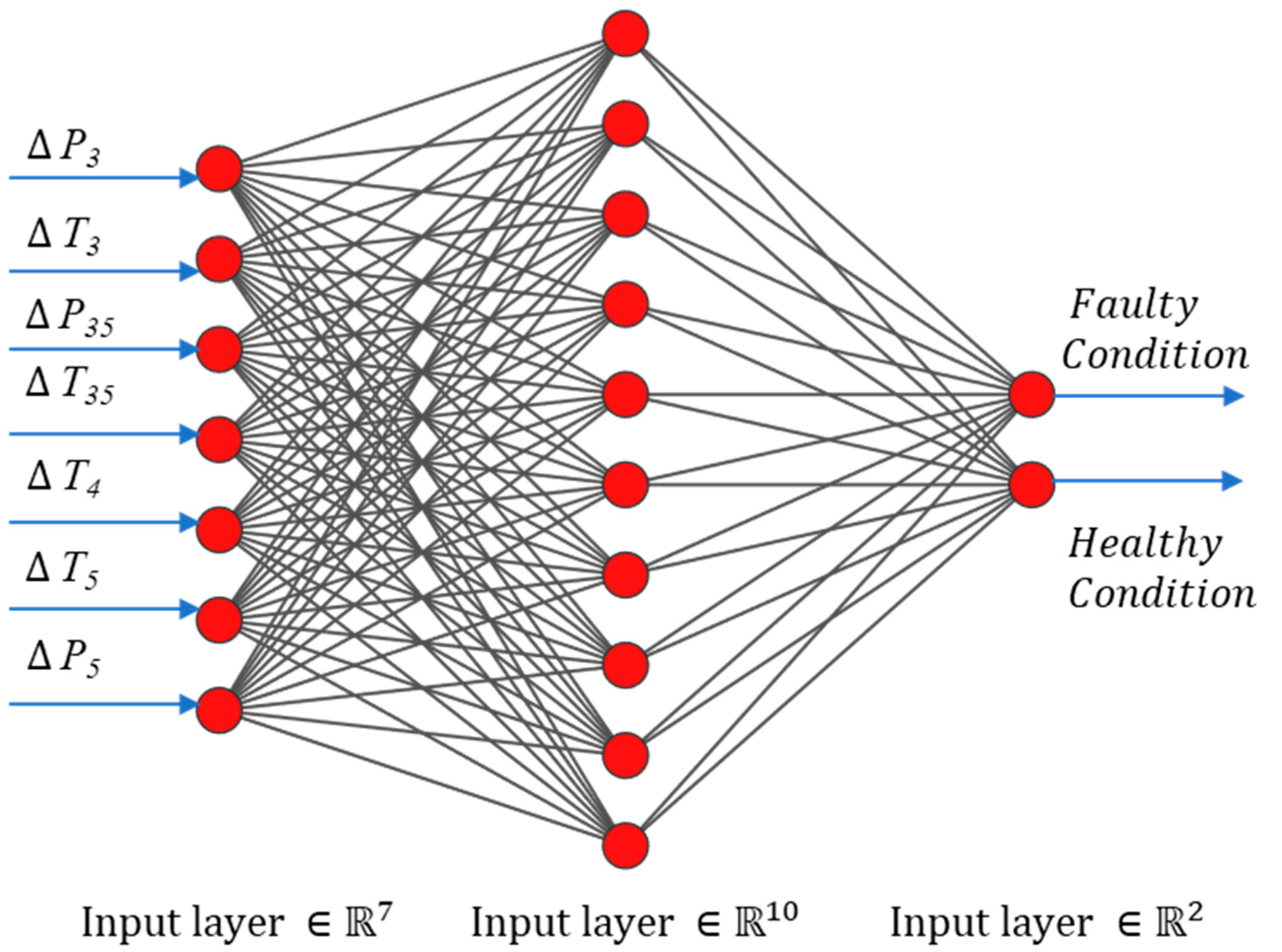
After accomplishing the preprocessing of the data, the data were fed into the ANN-based classification learner in the form of two separate datasets, i.e., NG and hydrogen, using the MATLAB tool. Using the scenarios involved in the labeled data, a classification algorithm “learned” about the classification of fresh observations through a supervised machine-learning approach. Although there are plenty of other algorithms for the classification learning, the ANN was chosen in the present study. The reason for choosing the ANN lies in the inherent ability of this algorithm to (i) efficiently capture the nonlinear behavior of the engine performance [9], (ii) extract information in a fast and simplistic way [36], (iii) handle multiple and larger component faults in the presence of sensor faults [43], (iv) deal with measurement uncertainties [6], and (v) perform the diagnosis with a scarcity of measurements [44]. The ANN architecture for both the fault detection and isolations are illustrated in Figure 7 and Figure 8. In the classification learner, a validation method needed to be chosen to assess the prediction accuracy of the fitted model. The validation not only provided performance estimations of the model on a completely new dataset (as compared to the training dataset), but also helped in protecting against overfitting. The validation scheme chosen in the present study was k -folds cross-validation. This scheme works by dissecting the training datasets into k disjoint sets or partitions, and then randomly shuffling them. For each round of training–validation, a certain partition was used for the validation, while the rest of the data were used for the testing. Therefore, each partition was used once for the validation, while the partitions were used k 1 times for the training. The k was assumed to be 5 in the present case based on the data samples. Cross-validation helps in avoiding the overfitting of the training data, so that the prediction accuracy might not be compromised.
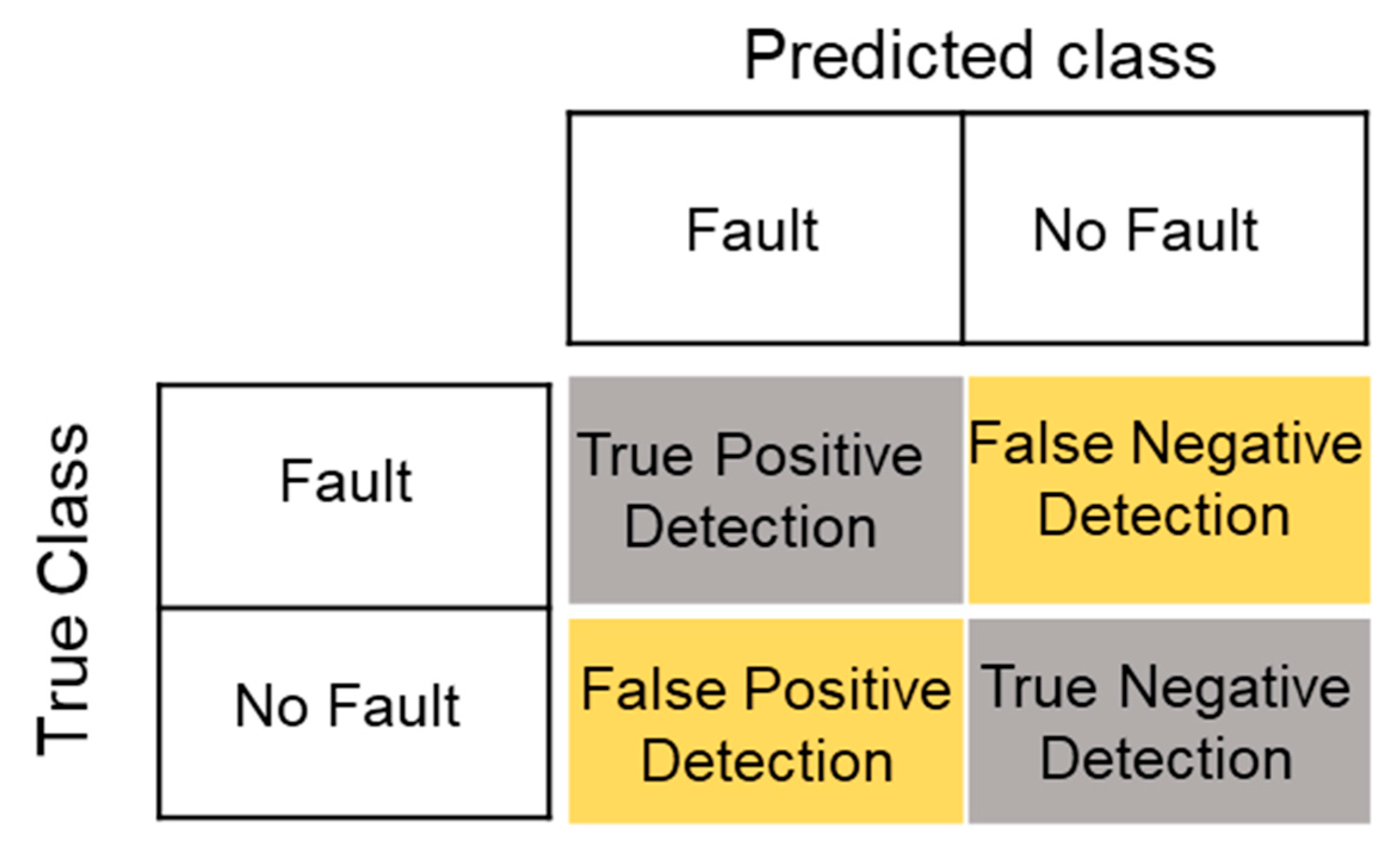
The classification algorithms finally provided a confusion matrix that determined the number of faults accurately predicted or wrongly predicted. The confusion matrix provided information about the performance of the selected classifier in each class, i.e., the true class or predicted class. The rows in the matrix show the true class, while the columns represent the predicted class. The diagonal cells depict the matching of both the true and predicted classes.

2.3.3. ANN-Based Fault Identification

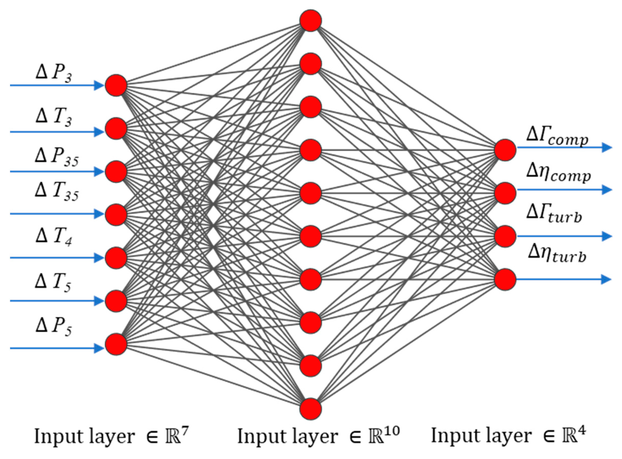
The final step involved in an MGT diagnosis process is fault identification. The present study utilizes a multilayer perceptron (MLP) for the intended component fault identification. The MLP is a kind of feedforward neural network that works on the concept of supervised learning, comprised of an input layer, an output layer, and one or more hidden layers. In the training phase of the ANN, the network manages to learn the correlations between the input and output data using a back-propagation algorithm. The current study utilized a single-layer MLP with 10 nodes, as shown in Figure 9. In general, the fault identification was carried out by tracing the health parameters, i.e., (flow capacity: Γ ; efficiency: η ) back from the deviated fault signatures. In Figure 9, on the left-hand side of the ANN structure, the inputs are provided that have been derived from Equation (5), while the outputs illustrated on the right-hand side of the structure have been derived from Equations (2) and (3). The terms with Δ in the figure represent the measurement deviations, while Γ and η represent the flow capacity and efficiency of the compressor and turbines, respectively. The network was trained on the three fault scenarios (CF, TC, and CF + TC) to identify some suitable relationships from the fed samples, thereby fine-tuning the weights and biases. The performance of the training or prediction accuracy was determined by the mean square error (MSE) by combining the results from both the training and validation datasets. The training progress data and model summary of the ANN algorithm have been listed in Table 4.

2.3.4. Explainable AI for Interpretation

The methodology further encompassed explainable artificial intelligence (XAI) to acquire useful physics-based interpretations from the ANN-based black-box model. Normally, SHAP (SHapley Additive exPlanations) values analysis is adopted to see the effect of different input features on the AI-based model outputs. In this way, SHAP helps in providing a true picture of a physical phenomenon present in any of the data and, furthermore, the influence of those physics-based parameters on the output of the model as the training evolves. The generic mathematical representation of the SHAP values has been provided in Equation (7),
φ j f , x = S F f s ! N S 1 ! N ! f x S j f x ( S )
where F and N represent the power set of all features and the total number of features, respectively, while the exclusion of feature j from the features creates a subset S . The term f x S j f x ( S ) is the expected marginal contribution of adding feature j to the feature subset S for sample x , necessitating model f to be evaluated again. The SHAP value is defined as the amount that feature j contributes to the prediction of sample x over and above the baseline average forecast or expectation. The most important characteristic of SHAP theory, local accuracy, is described in Equation (8), and asserts that the total of all attributions equals the prediction:
f x = φ 0 f + j = 1 N φ j ( f , x )
where φ 0 f is the model’s baseline prediction and f x is explained by a linear sum of the derived SHAP values.

3. Results and Discussion

3.1. Fault Detection and Isolation

For the fault detection and isolation, an ANN-based classifier was employed. Two kinds of datasets were trained, and three fault scenarios were accounted for. For each dataset, 70% of the data were utilized for the training, while the remaining 30% were employed for the testing and validation (15% for each) of the algorithm. The performance of the classification algorithm is normally assessed by the detection decision matrix and classification confusion matrix, consisting of the main decision metric parameters, i.e., the true positive (TP), false negative (FN), false positive (FP), and true negative (TN), as illustrated in Figure 10. The main diagonal depicts the correctly predicted faults, while the off diagonal shows the wrongly predicted elements. The detection rates of these decision parameters can be estimated through the normalization that is performed by dividing each matrix element by the sum of its row’s elements, as follows [45],
T P R = T P T P + F N × 100 %
F P R = F P F P + T N × 100 %
F N R = F N T P + F N × 100 %
T N R = T N F P + T N × 100 %
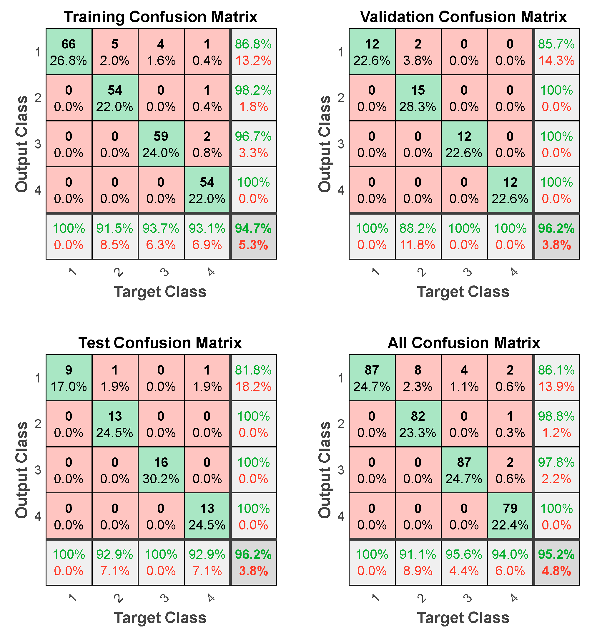
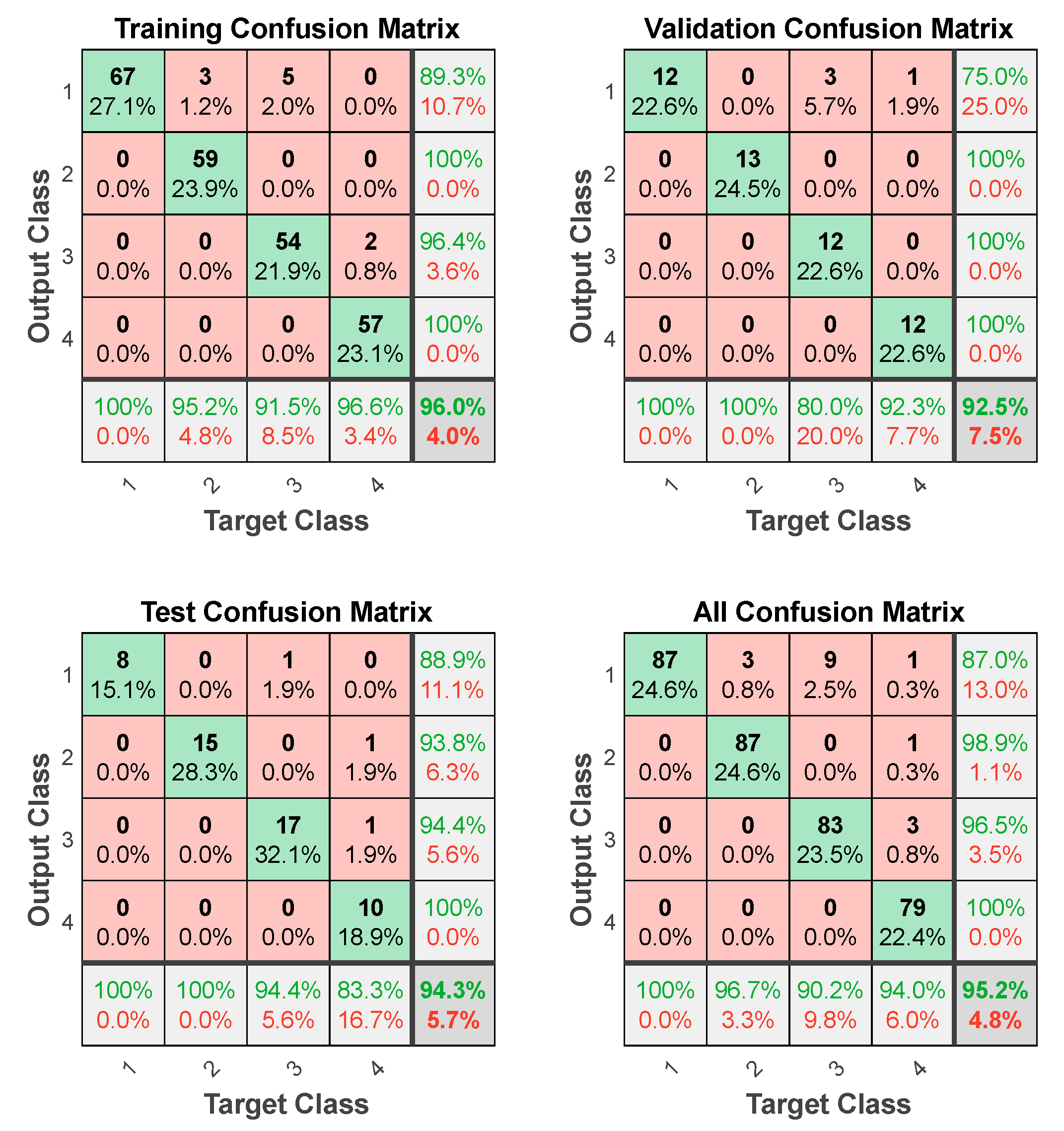
The selected classification algorithm enables the classification of multiple faults, as shown in Figure 11 and Figure 12. The figures represent the confusion matrix of the hydrogen and NG-fueled scenarios, respectively. The labels mentioned on the x- and the y-axes represent the different fault and no-fault conditions for the predicted and true classes, respectively, as listed in Table 5.
A detailed overview of the fault detection and isolation accuracy has been portrayed in Figure 11. The figure illustrates the confusion matrices of the training, validation, testing, and overall accuracies of the fault detection and isolation modules for the hydrogen-fueled scenario. The x-axis shows the target or the predicted class, while the y-axis shows the output or the true class of the variety of faults. It should be noted that correctly classified classes are represented in green color while misclassified classes are represented in red color. The overall classification accuracy of the training was found to be 94.7%. The training phase shows a classification accuracy of 86.8% for class 1, with some misclassification. Among those misclassifications, 2% of the data were misclassified as compressor fouling, while 1.6% and 0.4% of the data were misclassified as turbine corrosion and simultaneous compressor fouling and turbine corrosion, respectively. Similarly, for class 2 and class 3, some misclassifications were noticed. For instance, 0.4% of the data in class 2 were misclassified as simultaneous fouling and corrosion, while, in class 3, 0.8% of the data were misclassified as simultaneous compressor fouling and turbine corrosion. In the validation phase, class 1 misclassified 3.5% of the data as compressor fouling, while the rest of the classes showed 100% accuracy, thereby leading to an overall validation accuracy of 96.2%. Similarly, the classification accuracy of the testing phase was found to be 96.2%, with some misclassifications in class 1, in which 1.9% of the data were misclassified as compressor fouling, while 1.9% of the data were misclassified as simultaneous compressor fouling and turbine corrosion. Furthermore, a combination of all the confusion matrices has been illustrated as “all confusion matrix” and is displayed in Figure 11, which showed an accuracy of 95.2%. However, the testing accuracy provides true insights about the detection and isolation of the physical faults in the gas turbines.
Similarly, Figure 12 presents an overview of the classification accuracies of the NG-fueled scenario. As can be observed from the figure, class 1 shows an accuracy 89.3% with some misclassification, in which 1.2% of the data were wrongly classified as compressor fouling, while 2% of the data were wrongly classified as turbine corrosion. Similarly, class 3 also manifested misclassifications, in which 0.8% of the faults were wrongly classified as simultaneous compressor fouling and turbine corrosion. In the validation phase, class 1 misclassified 5.7% of the data as compressor fouling, while 1.9% of the faults were misclassified as simultaneous compressor fouling and turbine corrosion. The rest of the classes showed 100% accuracy, thereby leading an overall validation accuracy of 92.5%. The testing accuracy of the classification for the NG-fueled scenario was found to be 94.3%, which was slightly lower than that of the hydrogen-fueled gas turbine scenario. The reason for this has been illustrated in Figure 12, in terms of three misclassified faults. For instance, in class 1, 1.9% of the faults were misclassified as turbine corrosion. Similarly, class 2 and class 3 also represented some misclassified faults, such as 1.9% of the faults misclassified as simultaneous compressor fouling and turbine corrosion in each class. The overall confusion matrix accuracy was found to be 95.2%. The comparison of both the hydrogen-fueled and NG-fueled scenarios concluded that the training accuracy of the hydrogen-fueled scenario was marginally lower than the NG-fueled scenario, while the validation and testing accuracy of the hydrogen-fueled scenario was slightly higher than that of NG gas scenario. However, the accuracy of all confusion matrices for both fuel scenarios was surprisingly found to be same. It is important to note that, while dealing with fault detection, the testing accuracy of the algorithm maintains a higher prestige, since it serves as a deciding factor for the correctness of the classification algorithm for the unseen data.
During the fault detection, the presence of a hydrogen-based corrosion fault led to an increased level of incorrectly classified ‘no fault’ as hydrogen-induced corrosion fault. Moreover, the turbine corrosion fault prompted an extra fault as simultaneous compressor fouling and turbine corrosion in contrast with the NG case. This means that the presence of the hydrogen-induced corrosion fault might influence the fault detection process by producing a false alarm of the fault, while there is no actual fault in the training face of the algorithms. However, during the testing phase, the situations were reversed as compared to the NG scenario. Hence, the study further inferred that the presence of hydrogen-based steam-induced corrosion might lead to a few false alarms, thereby increasing the downtime of the asset and subsequently incurring preventive maintenance expenses.

3.2. Sensitivity Analysis for Fault Detection and Isolation

One of the biggest challenges that might arise while performing fault diagnostics is the inaccuracy of the fault detection modules due to the unavailability of certain measurement sensors in the actual engine provided by the OEM. The MGT engine considered in the present study also had a few measurement sensors that were originally installed by the OEM, such as the turbine inlet temperature (TIT), or T3, and the turbine outlet temperature (TOT), or T5. However, a variety of the new sensors were also installed on the engine for the effective condition monitoring and performance optimization of the engine for future purposes. The measurements considered in this study were conformed with the newly installed sensors. Moreover, the sensor measurements in the simulation were also reconciled with the same newly installed measurement sensors. Therefore, the absence of a few sensors on an engine provided by OEM might impact the fault diagnostic accuracy. In this regard, the sensitivity analysis of the fault detection and isolation accuracies is of paramount importance.
The sensitivity analysis involved in the present work was performed on the different sensor measurement parameters that were inherently made part of the fault diagnostics process. The sensitivity analysis was conducted with 10 different combinations of the measurements to investigate the influence of some dropped measurements on the overall testing accuracy of the fault diagnostics process. All the possible combinations along with fault diagnostic accuracies for both the hydrogen- and NG-fueled scenarios have been listed in Table 6. The sensitivity analysis manifests that the unavailability of some temperature measurements does not create much of an impact on the fault diagnostic accuracy, such as T3, T4, and T35. However, it is important to note that the unavailability of multiple measurement sensors significantly affects the accuracy. For instance, dropping T3 and T4 simultaneously reduced the fault diagnostic accuracy of the hydrogen-fueled MGT scenario (62.3%), while the accuracy of the NG-fueled scenario remained unaffected. It became evident that the fault diagnostic accuracy of the hydrogen-fueled scenario was more sensitive to the temperature-measurement sensors T3 and T4. Similarly, dropping a row of sensors led to a catastrophic drop in the accuracy; for example, the removal of T3, T35, T4, and T5 from the fault diagnostics features led to an accuracy reduction of 56.6%. The most important finding that was unleashed during the sensitivity analysis was the vulnerability of the fault diagnostic accuracy to some of the pressure sensors. For instance, the removal of P5 from the input feature led to a fault diagnostic accuracy reduction of 50.9%. The situation became even worse when a series of pressure-measurement sensors, i.e., P3, P35, and P5, were removed; the accuracy dropped to 47.2%.
The entire sensitivity analysis unleashed some new findings. One of the important findings is that the hydrogen-fueled scenario was more sensitive to the fault diagnostic accuracy when it came to the unavailability of the measurement sensors. The unavailability of multiple measurement sensors, both pressure- and temperature-based sensors, showed a drastic reduction in the fault diagnostic accuracy in the hydrogen-fueled scenario, whereas the NG-fueled scenario did not seem to be affected much by the unavailability of multiple temperature and pressure sensors. It is also worthy to note that dropping even some of the temperature sensors did not change the accuracy at all, such as the exclusion of T3 and T35. A strange behavior for the hydrogen-fueled scenario was also noticed when dropping P3; the removal of P3 led to an increase in the fault diagnostic accuracy. The findings of this study highlight the importance of some pressure- and temperature-measurement sensors for the accurate fault diagnostics of the hydrogen-fueled gas turbine scenario. Therefore, it is suggested to carry out an inspection before performing maintenance to avoid the risk of the malfunctioning of the measurement sensors, which might lead to potentially inaccurate fault diagnostics.

3.3. Fault Identification

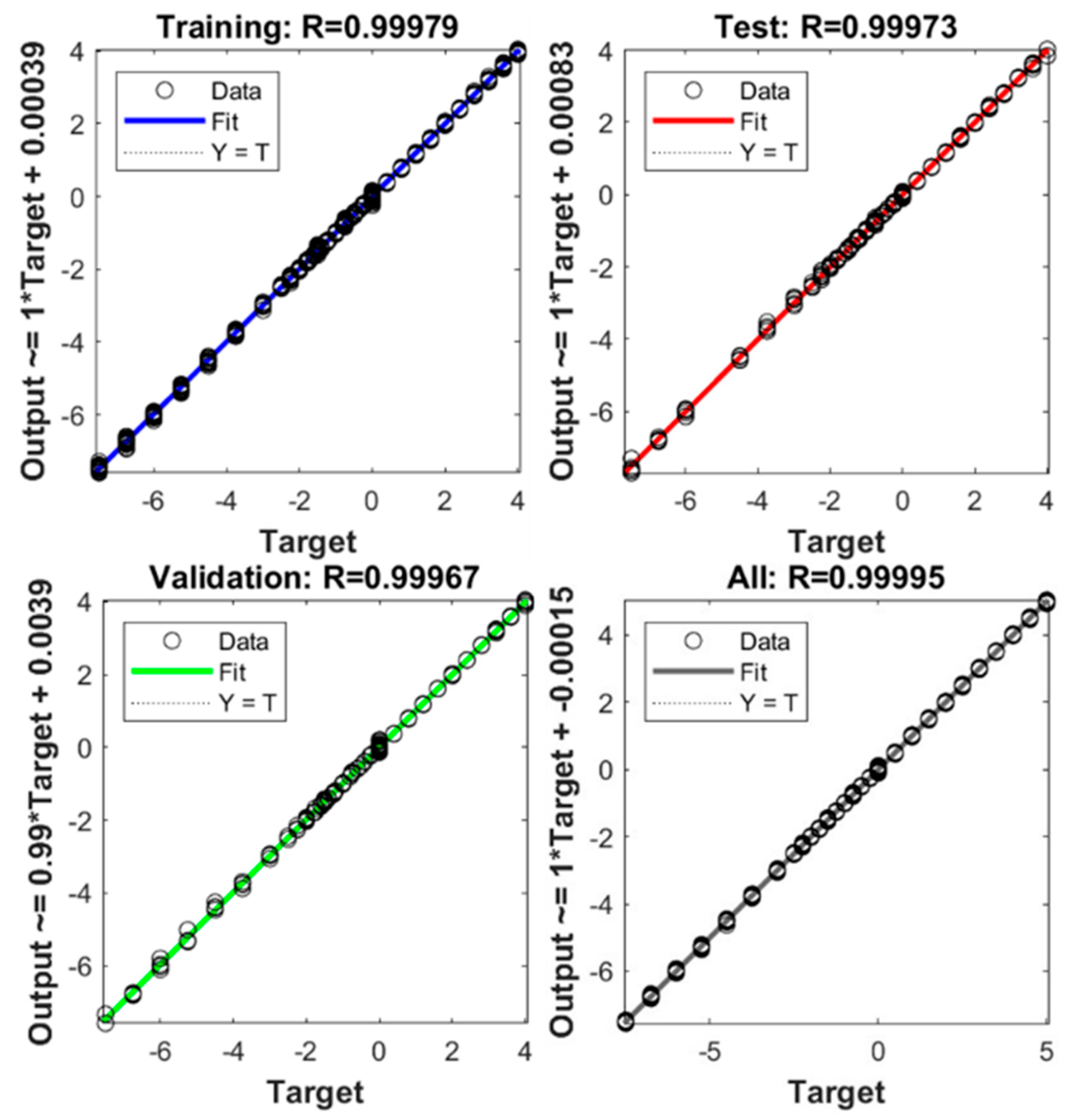
The fault identification of the MGT was carried out by using a feedforward neural network. The computational framework of the ANN based fault identification employed regression analysis. The regression plots of the training, testing, and validation are illustrated in Figure 13. The figure indicates that the ANN was able to identify the physical fault parameters with a quite good accuracy, since the regression values were almost close to 1. The performance of the ANN prediction is normally evaluated by the level of error minimization with respect to the number of epochs (cycles). An epoch is basically the training process of the ANN with all the available data at once for one cycle. It is always desirable to keep the accuracy as high as possible during the training.
Normally, a learning curve graph helps in visualizing the convergence of the training, testing, and validation; hence, it provides information about the accuracy in given epochs. The learning curve graph continues to improve until the model coverages with a minimized error, as shown in Figure 14.
The regression of both the NG- and hydrogen-fueled scenarios was found to be nearly identical, with a similar accuracy, as can be observed from Figure 15. The learning curve-based performance of the hydrogen-fueled scenario is shown in Figure 16. The error minimization of the hydrogen scenario took 404 epochs, which was significantly greater than that of the NG scenario, i.e., 202 epochs.
The overall accuracy of the ANN training, testing, and validation was determined by the root mean square error (RMSE) using Equation (13). The n involved in the equation expresses the total sample size, while p f and t f represent the predicted and target fault values. The results of both the MSE and RMSE between the predicted and target values for both the NG and hydrogen scenarios are listed in Table 7. It became evident that the RMSE of the training, testing, and validation phases of the hydrogen scenario was slightly higher than that of the NG scenario.
R M S E = M S E = 1 n i = 1 n p f t f 2
A list of different studies (including the current one) related to the fault diagnostics is presented in Table 8. The list includes studies dealing with some deep-learning and machine-learning algorithms for a variety of gas turbine engines, such as MGT, IGT, and aeroengines, using natural gas fuel. It should be noted that the accuracy of the algorithms is critically related to the corresponding gas turbine system configuration and the volume of the dataset. The accuracy of the present work was found to be 96.2% for the natural gas case. However, for the hydrogen scenario, this might be further decreased due to presence of false alarms and missed detections. Making a comparison between the current study and the one in [32], both considering MGTs, there is a small difference in the accuracy. The reason for this is the difference in the data size and the hyperparameters selected during the training of the algorithms.

3.4. Physics-Based Insights from the ANN Model

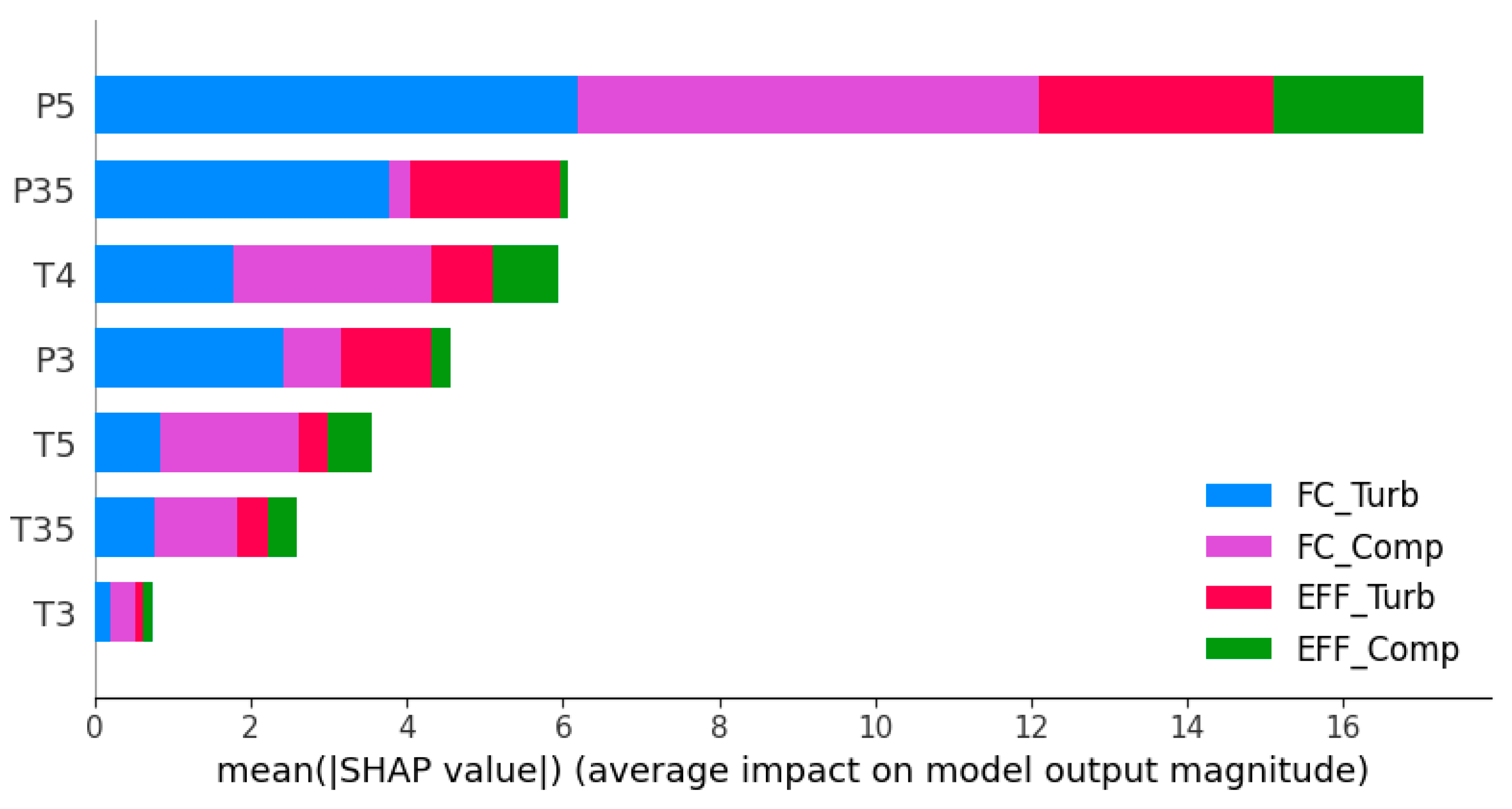
To acquire the physics-oriented insights from the ANN-based black-box model, XAI-based SHAP (SHapley Additive exPlanations) values were utilized. Figure 17 illustrates a feature importance bar plot that explains the influence of different input parameters on the model parameters. The average impact of the model output magnitude has been depicted by calculating mean SHAP values of all the input features. The spread of the bars reveals that input features, such as P5, P35, and T4, had a significant contribution in the fault diagnostics model. However, the contribution of the input feature P5 was one of the dominant features in the model output prediction. In prediction of the output characteristics of the diagnostic model, the compressor flow capacity and turbine flow capacity were found to be significantly affecting to the P5 feature, while the contribution of the compressor efficiency and turbine efficiency was comparatively small. The reason for this is supported by the fact that, during the physics-based model development, the magnitudes of the compressor and turbine isentropic efficiencies were assumed to be smaller than that of the flow capacity magnitudes. It is also worth noticing that the features consisting of the pressure terms have the turbine flow capacity as the dominant factor in the SHAP values, represented by a blue color. The results from the SHAP values are quite well in agreement with the sensitivity analysis results elaborated in Section 3.2.

4. Conclusions

This study aimed at developing a fault diagnosis model for a hydrogen-fueled MGT in comparison with an NG-fueled case. The study involved the development of a physics-based model for data generation as an initial step. The data further went through a preprocessing phase prior to the fault detection, isolation, and identification. Fault detection and isolation were carried out using an ANN-based classification learner, while the fault identification was performed using an MLP feedforward ANN. The detection and isolation module showed greater percentages of wrongly classified faults due to the involvement of steam-induced corrosion in the hydrogen-fueled scenario as compared to an NG-fired MGT. The performance of the fault identification was, however, found to be similar for both the NG- and hydrogen-based scenarios. Further work is needed with increased levels of fault severity arising due to steam-induced corrosion for better fault identification in hydrogen-fueled scenarios. This study was part of an initial attempt towards the fault diagnosis of hydrogen-fueled micro gas turbines. However, further advancements might help design and maintenance engineers assure the optimum reliability and availability of the MGT.

Author Contributions

Conceptualization, M.B.H.; methodology, M.B.H.; software, M.B.H.; validation, M.B.H.; formal analysis, M.B.H.; investigation, M.B.H.; resources, M.B.H. and M.M.; data curation, M.B.H. and A.D.F.; writing—original draft preparation, M.B.H. and S.A.; writing—review and editing, M.B.H., M.M. and S.A.; visualization, M.B.H.; supervision, M.M., A.D.F. and K.K.; project administration, M.M.; funding acquisition, M.M. All authors have read and agreed to the published version of the manuscript.

Funding

This research was funded through the Equinor-UiS Academia Agreement.

Data Availability Statement

The data presented in this study are available on request from the corresponding author.

Acknowledgments

The authors would like to thank the University of Stavanger and the Equinor’s Academia Agreement for providing invaluable support in conducting this research. Mohammad Mansouri would like to acknowledge the Robinson project, which received funding from the European Union’s Horizon 2020 research and innovation programme under grant agreement no. 957752. It should be noted that this paper reflects only the authors’ views, and the Research Executive Agency, Equinor ASA, and the European Commission are not liable for any use that may be made of the information contained therein.

Conflicts of Interest

The authors declare no conflicts of interest.

References

  1. EDGAR; JRC. Global Carbon Dioxide Emissions from 1970 to 2021, by Sector (in Billion Metric Tons of Carbon Dioxide); Statista: Hamburg, Germany, 2022. [Google Scholar]
  2. ETN Global. Zero-carbon gas turbine. In Hydrogen Gas Turbines; ETN Global: Brussels, Belgium, 2020. [Google Scholar]
  3. Noble, D.; Wu, D.; Emerson, B.; Sheppard, S.; Lieuwen, T.; Angello, L. Assessment of current capabilities and near-term availability of hydrogen-fired gas turbines considering a low-carbon future. J. Eng. Gas Turbines Power 2021, 143, 041002. [Google Scholar] [CrossRef]
  4. Siemens Energy; Centrax. HYFLEXPOWER Consortium Successfully Operates a Gas Turbine with 100 Percent Renewable Hydrogen, a World First; Siemens Energy: Munich, Germany, 2023. [Google Scholar]
  5. Gazzani, M.; Chiesa, P.; Martelli, E.; Sigali, S.; Brunetti, I. Using hydrogen as gas turbine fuel: Premixed versus diffusive flame combustors. J. Eng. Gas Turbines Power 2014, 136, 051504. [Google Scholar] [CrossRef]
  6. Marinai, L.; Probert, D.; Singh, R. Prospects for aero gas-turbine diagnostics: A review. Appl. Energy 2004, 79, 109–126. [Google Scholar] [CrossRef]
  7. Urban, L.A. Parameter selection for multiple fault diagnostics of gas turbine engines. J. Eng. Power 1975, 97, 225–230. [Google Scholar] [CrossRef]
  8. Urban, L.A.; Volponi, A.J. Mathematical methods of relative engine performance diagnostics. SAE Trans. 1992, 101, 2025–2050. [Google Scholar]
  9. Fentaye, A.D.; Baheta, A.T.; Gilani, S.I.; Kyprianidis, K.G. A review on gas turbine gas-path diagnostics: State-of-the-art methods, challenges and opportunities. Aerospace 2019, 6, 83. [Google Scholar] [CrossRef]
  10. Minghui, H.; Ya, H.; Xinzhi, L.; Ziyuan, L.; Jiang, Z.; Bo, M. Digital twin model of gas turbine and its application in warning of performance fault. Chin. J. Aeronaut. 2022, 36, 449–470. [Google Scholar]
  11. Chen, Y.-Z.; Zhao, X.-D.; Xiang, H.-C.; Tsoutsanis, E. A sequential model-based approach for gas turbine performance diagnostics. Energy 2021, 220, 119657. [Google Scholar] [CrossRef]
  12. Kim, S.; Im, J.H.; Kim, M.; Kim, J.; Kim, Y.I. Diagnostics using a physics-based engine model in aero gas turbine engine verification tests. Aerosp. Sci. Technol. 2023, 133, 108102. [Google Scholar] [CrossRef]
  13. Ying, Y.; Li, J. An improved performance diagnostic method for industrial gas turbines with consideration of intake and exhaust system. Appl. Therm. Eng. 2023, 222, 119907. [Google Scholar] [CrossRef]
  14. He, Y.; Jiang, Z.; Hu, M.; Li, Y. Local maximum synchrosqueezing chirplet transform: An effective tool for strongly nonstationary signals of gas turbine. IEEE Trans. Instrum. Meas. 2021, 70, 1–14. [Google Scholar] [CrossRef]
  15. Chen, Y.-Z.; Tsoutsanis, E.; Wang, C.; Gou, L.-F. A time-series turbofan engine successive fault diagnosis under both steady-state and dynamic conditions. Energy 2023, 263, 125848. [Google Scholar] [CrossRef]
  16. Zhou, H.; Ying, Y.; Li, J.; Jin, Y. Long-short term memory and gas path analysis based gas turbine fault diagnosis and prognosis. Adv. Mech. Eng. 2021, 13, 16878140211037767. [Google Scholar] [CrossRef]
  17. Yang, X.; Bai, M.; Liu, J.; Liu, J.; Yu, D. Gas path fault diagnosis for gas turbine group based on deep transfer learning. Measurement 2021, 181, 109631. [Google Scholar] [CrossRef]
  18. Zhou, D.; Yao, Q.; Wu, H.; Ma, S.; Zhang, H. Fault diagnosis of gas turbine based on partly interpretable convolutional neural networks. Energy 2020, 200, 117467. [Google Scholar] [CrossRef]
  19. Shen, Y.; Khorasani, K. Hybrid multi-mode machine learning-based fault diagnosis strategies with application to aircraft gas turbine engines. Neural Netw. 2020, 130, 126–142. [Google Scholar] [CrossRef] [PubMed]
  20. Bai, M.; Liu, J.; Ma, Y.; Zhao, X.; Long, Z.; Yu, D. Long short-term memory network-based normal pattern group for fault detection of three-shaft marine gas turbine. Energies 2020, 14, 13. [Google Scholar] [CrossRef]
  21. Montazeri-Gh, M.; Yazdani, S. Application of interval type-2 fuzzy logic systems to gas turbine fault diagnosis. Appl. Soft Comput. 2020, 96, 106703. [Google Scholar] [CrossRef]
  22. Zhu, L.; Liu, J.; Ma, Y.; Zhou, W.; Yu, D. A coupling diagnosis method for sensor faults detection, isolation and estimation of gas turbine engines. Energies 2020, 13, 4976. [Google Scholar] [CrossRef]
  23. Cao, Y.; Luan, J.; Han, G.; Lv, X.; Li, S. A marine gas turbine fault diagnosis method based on endogenous irreversible loss. Energies 2019, 12, 4677. [Google Scholar] [CrossRef]
  24. Li, J.; Ying, Y. Gas turbine gas path diagnosis under transient operating conditions: A steady state performance model based local optimization approach. Appl. Therm. Eng. 2020, 170, 115025. [Google Scholar] [CrossRef]
  25. Sun, R.; Shi, L.; Yang, X.; Wang, Y.; Zhao, Q. A coupling diagnosis method of sensors faults in gas turbine control system. Energy 2020, 205, 117999. [Google Scholar] [CrossRef]
  26. Zhong, S.-S.; Fu, S.; Lin, L. A novel gas turbine fault diagnosis method based on transfer learning with CNN. Measurement 2019, 137, 435–453. [Google Scholar] [CrossRef]
  27. Gomes, E.; McCaffrey, D.; Garces, M.; Polizakis, A.; Pilidis, P. Comparative analysis of microturbines performance deterioration and diagnostics. In Proceedings of the Turbo Expo: Power for Land, Sea, and Air, Barcelona, Spain, 8–11 May 2006; pp. 269–276. [Google Scholar]
  28. Yoon, J.E.; Lee, J.J.; Kim, T.S.; Sohn, J.L. Analysis of performance deterioration of a micro gas turbine and the use of neural network for predicting deteriorated component characteristics. J. Mech. Sci. Technol. 2008, 22, 2516. [Google Scholar] [CrossRef]
  29. Talebi, S.; Tousi, A. The effects of compressor blade roughness on the steady state performance of micro-turbines. Appl. Therm. Eng. 2017, 115, 517–527. [Google Scholar] [CrossRef]
  30. Bauwens, P. Gas Path Analysis for the MTT Micro Turbine; TU Delft: Delft, The Netherlands, 2015. [Google Scholar]
  31. Hashmi, M.B.; Mansouri, M.; Breuhaus, P.; Lemma, T.A. Effect of hot gas path component corrosion on the performance of hydrogen fueled micro gas turbines. In Proceedings of the Turbo Expo: Power for Land, Sea, and Air, Boston, MA, USA, 26–30 June 2023; p. V009T018A016. [Google Scholar]
  32. Talebi, S.; Madadi, A.; Tousi, A.; Kiaee, M. Micro Gas Turbine fault detection and isolation with a combination of Artificial Neural Network and off-design performance analysis. Eng. Appl. Artif. Intell. 2022, 113, 104900. [Google Scholar] [CrossRef]
  33. Zornek, T.; Monz, T.; Aigner, M. Performance analysis of the micro gas turbine Turbec T100 with a new FLOX-combustion system for low calorific fuels. Appl. Energy 2015, 159, 276–284. [Google Scholar] [CrossRef]
  34. Kurzke, J. GasTurb 12: A Program to Calculate Design and Off-Design Performance of Gas Turbines: User’s Manual; GasTurb: Aachen, Germany, 2012. [Google Scholar]
  35. Turbec, S. Technical Description Microturbine Turbec T100: Stand. 2017. Available online: https://manualzz.com/doc/33686173/t100-microturbine-system-technical-description-t100-natur (accessed on 1 January 2024).
  36. Tahan, M.; Tsoutsanis, E.; Muhammad, M.; Karim, Z.A. Performance-based health monitoring, diagnostics and prognostics for condition-based maintenance of gas turbines: A review. Appl. Energy 2017, 198, 122–144. [Google Scholar] [CrossRef]
  37. Oluyede, E.O.; Phillips, J.N. Fundamental impact of firing syngas in gas turbines. In Proceedings of the Turbo Expo: Power for Land, Sea, and Air, Barcelona, Spain, 8–11 May 2007; pp. 175–182. [Google Scholar]
  38. Zwebek, A.; Pilidis, P. Degradation effects on combined cycle power plant performance—Part III: Gas and steam turbine component degradation effects. J. Eng. Gas Turbines Power 2004, 126, 306–315. [Google Scholar] [CrossRef]
  39. Zwebek, A.; Pilidis, P. Degradation Effects on Combined Cycle Power Plant Performance—Part II: Steam Turbine Cycle Component Degradation Effects. J. Eng. Gas Turbines Power 2003, 125, 658–663. [Google Scholar] [CrossRef]
  40. Qingcai, Y.; Li, S.; Cao, Y.; Zhao, N. Full and part-load performance deterioration analysis of industrial three-shaft gas turbine based on genetic algorithm. In Proceedings of the ASME Turbo Expo 2016: Turbomachinery Technical Conference and Exposition, Seoul, Republic of Korea, 13–17 June 2016; p. V006T005A016. [Google Scholar]
  41. Mohammadi, E.; Montazeri, G.M. Simulation of full and part-load performance deterioration of industrial two-shaft gas turbine. J. Eng. Gas Turbines Power 2014, 136, 092602. [Google Scholar] [CrossRef]
  42. Escher, P. Pythia: An Object-Orientated Gas Path Analysis Computer Program for General Applications; Cranfield University: Cranfield, UK, 1995. [Google Scholar]
  43. Ogaji, S.O.; Singh, R. Advanced engine diagnostics using artificial neural networks. Appl. Soft Comput. 2003, 3, 259–271. [Google Scholar] [CrossRef]
  44. Singh, R. Advances and opportunities in gas path diagnostics. In Proceedings of the 15th ISABE, Bangalore, India, 17–20 September 2003. Paper no. ISABE-2003-1008. [Google Scholar]
  45. Simon, D.L. Propulsion Diagnostic Method Evaluation Strategy (ProDiMES) User’s Guide; NASA: Washington, DC, USA, 2010.
Figure 1. The methodology workflow.
Energies 17 00719 g001
Figure 2. Schematic of a 100 kW MGT.
Energies 17 00719 g002
Figure 3. Shaft speed at different part-load power settings.
Energies 17 00719 g003
Figure 4. Various temperatures at different part-load power settings.
Energies 17 00719 g004
Figure 5. Various pressures at different part-load power settings.
Energies 17 00719 g005
Figure 6. Various temperatures at part-load power settings.
Energies 17 00719 g006
Figure 7. ANN architecture along with the labeled data for the fault detection module.
Energies 17 00719 g007
Figure 8. ANN architecture with the labeled data for the fault isolation module.
Energies 17 00719 g008
Figure 9. Single-layer MLP architecture for the fault identification module.
Energies 17 00719 g009
Figure 10. Fault detection decision matrix.
Energies 17 00719 g010
Figure 11. Confusion matrix for the fault detection and isolation during the hydrogen-fueled scenario.
Energies 17 00719 g011
Figure 12. Confusion matrix for the fault detection and isolation during the NG-fueled scenario.
Energies 17 00719 g012
Figure 13. Regression plots for the training, testing, and validation of an NG fuel ANN model.
Energies 17 00719 g013
Figure 14. Performance of the ANN training for the NG-fueled scenario.
Energies 17 00719 g014
Figure 15. Regression plots for training, testing, and validation of a hydrogen-fueled ANN model.
Energies 17 00719 g015
Figure 16. Performance of the ANN training for the hydrogen-fueled scenario.
Energies 17 00719 g016
Figure 17. Effect of the input features on the model output.
Energies 17 00719 g017
Table 1. Gas turbine fault diagnostics studies in the past five years.
Ref.Engine TypeFaults/Degraded
Components
Diagnosis PhaseApproachSpecific Method
[15]Turbofan engineFan, compressor, and turbineFDIModel-basedNewton–Raphson
[11]Three-shaft IGTFouling and erosion in both compressors and turbinesFDIImproved nonlinear GPASequential diagnostics
[16]Single-shaft heavy-duty gas turbineFouling, erosion, corrosion, and blade rubbing; thermal distortion and local object damage in the compressor and turbineFDHybridLSTM and GPA
[17]Single-shaft IGTFouling and erosion in the compressor and turbineFDIIData-drivenCNN, DNN, and SVM
[18]MGTSensor fault and fouling in the compressorFDPhysics-based model + data-drivenCNN + Extreme gradient boosting (XGBoost)
[19]Twin-shaft aeroengineDegradation in the HPC, HPT, LPC, and LPTFDIHybrid machine-learningRNN
[20]Three-shaft marine GTFouling, and foreign object damage in the compressor and turbineFDData-drivenLSTM
[21]Twin-shaft IGTFouling and erosion in the compressor and turbineFDIPhysics-based model + data-drivenInterval type-two fuzzy logic systems
[22]Twin-shaft gas turbineSensor faultsFDIIHybrid model-based and unsupervised learningSRCKF + DBSCAN
[23]Three-shaft marine GTExergy loss in the compressor and turbineFDModel-basedEIL
[24]Single-shaft IGTFouling, erosion, corrosion, and blade rubbing; thermal distortion and object damage in the compressor and turbinesFDModel-basedKalman filter and Newton–Raphson algorithm
[25]IGTSensor faultsFDIData-drivenWavelet energy entropy and SVR
[26]Turbofan engineExhaust gas temperature-indication fault and HPT blade-burnt fault in the turbineFDIIData-drivenCNN and SVM
IGT: industrial gas turbine, HPC: high-pressure compressor, LPC: low-pressure compressor, HPT: high-pressure turbine, LPT: low-pressure turbine, FDI: fault detection and isolation, FDII: fault detection, isolation, and identification, LSTM: long short-term memory, SRCKFs: square-root cubature Kalman filters, DBSCAN: density-based spatial clustering of the application with noise, EIL: endogenous irreversible loss, CNN: convolutional neural network, DNN: dynamic neural network, GT: gas turbine, and SVM: support vector machine.
Table 2. Design-point validation after the optimization.
ParameterOEM Data [35]Present Study% Error
Power output [kW]100 (±3)100.10.09
Electrical efficiency [%]30 (±1)29.990.03
Pressure ratio [−]4.54.50
Exhaust mass flow0.80.7990.12
Exhaust gas temperature [K]543556.832.5
Table 3. Quantification of the various physical faults.
FaultFC (X)Eff. (Y)Ratios (X:Y)RangesRef.
Natural gas case
CF Γ c η t ~3:1[0, −7.5]
[0, −2.5]
[40,41]
TC Γ t η t ~2:1[0, 4]
[0, −2]
[42]
Hydrogen case
CF Γ c η t ~3:1[0, −7.5]
[0, −2.5]
[40,41]
TC Γ t η t ~2:1[0, 5]
[0, −2.5]
[27,39]
FC: flow capacity; Eff.: isentropic efficiency; CF: compressor fouling; TC: turbine corrosion; ↑: increasing; ↓: decreasing.
Table 4. ANN training progress data and model summary.
CriteriaIndicators
Total hidden layers1
Neurons in hidden layers10
Feeding approachBackpropagation
Target limit of epochs1000
Performance accuracy target0
Performance gradient target1.00 × 10−7
Activation functionSigmoid
Training algorithmLevenberg–Marquardt
Performance indicatorMean square error
Table 5. Labels of the different physical conditions in the classification algorithm.
LabelDesignated Physical Condition
1No fault
2CF: Compressor fouling
3TC: Turbine corrosion
4CF + TC: Simultaneous
Table 6. Sensitivity analysis of the fault diagnostics.
Sensitivity Measurement Sensors DroppedTesting Accuracy (%)—H2Testing Accuracy (%)—NG
S1T494.394.3
S2T4, T362.396.2
S3T394.392.5
S4T3592.596.2
S5T3, T3594.396.2
S6P396.292.5
S7P3592.590.6
S8P550.960.7
S9P3, P35, P547.254.7
S10T3, T35, T4, T556.662.3
Table 7. Analysis of the fault identification results in terms of the RMSE.
MSE NGMSE HydrogenRMSE NGRMSE Hydrogen
Training5.92 × 10−40.00180.02430.0424
Testing6.41 × 10−40.00220.02530.04694
Validation7.40 × 10−40.00320.02710.0565
Table 8. List of fault diagnostics studies in the literature, along with the present work.
Ref.SystemMethodologyFD Accuracy (%)
Current studyMGTANN96.2
[32]MGTANN97.6
[16]Heavy-duty gas turbineLSTM
[18]MGTCNN95.5
[19]aeroengineRNN89
[21]IGTFuzzy logic99
[26]Turbofan engineTransfer learning-based CNN and SVM93
Disclaimer/Publisher’s Note: The statements, opinions and data contained in all publications are solely those of the individual author(s) and contributor(s) and not of MDPI and/or the editor(s). MDPI and/or the editor(s) disclaim responsibility for any injury to people or property resulting from any ideas, methods, instructions or products referred to in the content.