Article

Planning of Reserve Storage to Compensate for Forecast Errors

by
Julian Koch
1,
Astrid Bensmann
1,*,
Christoph Eckert
1,
Michael Rath
2,3,† and
Richard Hanke-Rauschenbach
1
1
Institute of Electric Power Systems, Leibniz Universität Hannover, 30167 Hanover, Germany
2
Department of Civil and Environmental Engineering, Hochschule Bochum—Bochum University of Applied Sciences, 44801 Bochum, Germany
3
Fraunhofer Institution for Energy Infrastructures and Geothermal Systems IEG, 44801 Bochum, Germany
*
Author to whom correspondence should be addressed.
On Leave of GASAG Solution Plus GmbH, 10829 Berlin, Germany.
Energies 2024, 17(3), 720; https://doi.org/10.3390/en17030720
Submission received: 2 January 2024 / Revised: 26 January 2024 / Accepted: 30 January 2024 / Published: 2 February 2024
(This article belongs to the Section D: Energy Storage and Application)

Abstract

:
Forecasts and their corresponding optimized operation plans for energy plants never match perfectly, especially if they have a horizon of several days. In this paper, we suggest a concept to cope with uncertain load forecasts by reserving a share of the energy storage system for short-term balancing. Depending on the amount of uncertainty in the load forecasts, we schedule the energy system with a specific reduced storage capacity at the day-ahead market. For the day of delivery, we examine the optimal thresholds when the remaining capacity should be used to balance differences between forecast and reality at the intraday market. With the help of a case study for a simple sector-coupled energy system with a demand for cooling, it is shown that the energy costs could be reduced by up to 10% using the optimal reserve share. The optimal reserve share depends on the forecast quality and the time series of loads and prices. Generally, the trends and qualitative results can be transferred to other systems. However, of course, an individual evaluation before the realization is recommended.

1. Introduction

The subject of the current paper is electricity purchasing and scheduling different components of a sector-coupled energy system at the day-ahead and intraday market, considering uncertain load forecasting. The topic is important because even if the purchasing at day-ahead electricity markets operates perfectly, deviations of the load from the forecast will necessitate short-term balancing transactions at an intraday market. Depending on the deviation, these can be economically disadvantageous.
The optimal dispatch problem of energy systems is a classical research topic addressed in several review papers about energy management systems [1,2]. The most prominent approaches are optimization based. Therefore, the scheduling problem is solved either for the considered scheduling horizon (e.g., Nemati et al. [3], Li et al. [4]) or for a receding horizon via model predictive control (e.g., Kaya et al. [5]). In the latter one, uncertainties in load forecasts are either explicitly addressed via robust control [6,7,8] or compensated in a subsequent step, e.g., the real-time operation [9,10]. If multiple horizons are considered, such as day-ahead and real-time operation, hierarchical model predictive control is often used [5,9,11]. In contrast with these scientific efforts, rule-based strategies are often used for implementation. These have the advantage that they are not based on frequently deviating forecasts and are also easy to implement [12]. Generally speaking, simple algorithms are repeatedly evaluated to determine the scheduling. For example, a threshold value is often set for buying or selling energy and is compared with the current market price. In this context, for example, Ejeh et al. [12] proposes a methodology to define the optimal charging and discharging electricity price for electrical energy storage systems.
The current literature analyzes different energy systems under various market conditions. If an electricity market is considered, it is mainly modeled via fluctuating price signals such as the day-ahead market or intraday market [13]. Some authors focus on purely electric components such as photovoltaic power plants (PV), wind turbines, or batteries, e.g., Nemati et al. [3], Zhuang et al. [14]. In contrast, others investigate sector-coupled multienergy systems with additional heating or cooling demands, incorporating components such as combined heat and power plants (CHP), heat pumps, compression chillers, and thermal storage systems [5,8,15,16,17,18]. Even chemical plants such as air separation units have been considered in [19,20]. Vasilj et al. [6] consider a market for district heating, and Chen and Garcia [21] a generic setting with different markets for different goods such as steam. In contrast with the approaches mentioned above, some studies also explicitly address several electricity markets, where electricity is traded at different sequential closing times for a specific fulfillment date. Most prominently, the day-ahead and intraday markets are analyzed by Yin et al. [22], Xu et al. [23], Ji et al. [24], and Abdeltawab et al. [25], but Nguyen Duc and Nguyen Hong [26] also address balance capacity. Again, most authors focus on electrical systems, and only a few analyze sector-coupled energy systems. For example, [9] investigates a system consisting of a PV and a CHP controlled by a hierarchical control algorithm, and Wang et al. [10] analyze multistage energy management for a system consisting of a CHP, electric boiler, PV, and wind turbines and electrical and thermal storage systems.
In the present paper, we analyze a setting with two sequential electricity markets, the day-ahead and intraday markets, and a sector-coupled energy system with a demand for cooling from an existing plant [18] and cold storage system, focusing on handling uncertain load forecasts. As stated, this setting has seldom been analyzed before. Due to the discussed issues within the realization of only optimization-based strategies, we analyze a setting that is optimization based at the day-ahead market and rule based for the intraday operation. Therefore, an easy-to-implement realization of the intraday operation is ensured. Part of the energy storage system is treated as reserve storage to provide flexibility in the short-term balancing of forecast errors. This reserve part is not used at the day-ahead market. Chen and Garcia [21] use a similar approach regarding reserve storage but analyze another system setup.
In the analyzed system setup, there is a general trade-off between the flexibility at the day-ahead market and the ability to compensate for deviations between forecast and reality. Therefore, we want to investigate the following research questions: (1) Under which conditions in terms of prognosis quality does the reservation of reserve storage capacity make sense? (2) How large should this reserve storage share be, depending on the forecast quality? We analyze a simple sector-coupled energy system to answer these questions and show the idea behind the method and the potential of reserve storage. However, the method can be transferred to any sector-coupled or multienergy system, including a storage system in any infrastructure. The case study is based on an actual application in the form of an office campus.
In all, the contribution of the present paper can be summarized as follows:
  • Formal definition of the approach to reserve a storage share for short-term operation;
  • Model-based evaluation with a simple sector-coupled energy system and systematically generated load profiles;
  • Quantification of the potential of the proposed method and the corresponding necessary reserve share with a real case study.
The paper is structured as follows: Section 2 presents the general approach and underlying model of the considered system, as well as the methods for trading in both markets of interest. In Section 3, the focus is on evaluating the base case for generated load curves and variable dimensions. The results are compared with measured data for verification in Section 4.

2. General Approach, Methods, and Model

This section discusses the general approach, the necessary definitions, and model equations. The investigated example system and the corresponding model equations are introduced in the second part. Lastly, the concrete procedure for purchasing electricity and the storage system’s operation is defined.

2.1. General Approach

We consider two electricity markets, i.e., the day-ahead market and the continuous trading within the intraday market. However, the proposed method can also be applied to similar market settings. The uncertainty of a load forecast could be compensated by holding reserve storage for the operation of the plant and short-term action at the intraday market. In the following, the term load curve means time series in demands of cold.
Figure 1 shows a sketch of the present approach. In the first step, electricity is purchased from the day-ahead market based on a load forecast. From this, the costs at the day-ahead market and a day-ahead schedule for the system operation are identified. Moreover, in the second step, the actual load curve has to be fulfilled, and short-term compensation trades have to be performed, considering the short-term prices at the intraday market. The steps are explained in detail in the following.

2.1.1. Electricity Purchasing on Day-Ahead Market

Time series for load forecasts and knowledge about the quality and uncertainty of these are the basis for purchasing electricity at the day-ahead market. Depending on the forecast quality, parts of the storage system are not included in the trading strategy. However, they are kept as reserve storage for short-term deviations from the load forecast. In practice, this can be done for a thermal storage system by lowering its maximal temperature set point and raising its minimal temperature set point, resulting in a less usable energy capacity (c.f. reserve in the upper and lower parts of the storage system). With this information, the operation power of the components is planned, and the necessary electricity is purchased on the day-ahead market.
In the present paper, the trading strategy at the day-ahead market is not the focus. However, it must be taken into account to pay for the reduction in flexibility by setting reserve storage. Therefore, an optimization-based approach with a perfect prediction of day-ahead energy prices is used here. Details regarding this implementation are discussed in Section 2.2.

2.1.2. Operation and Trades at Intraday Market

In the second step, the schedule for the single components needs to be updated based on the actual load curves, which can differ from the load forecast. Therefore, the previously defined reserve storage is used, and additional trades at the intraday market can be placed (c.f. Figure 1). In this step, any advanced control strategies could be used. The present analysis uses a rule-based control approach. Section 2.2 gives detailed definitions for the selected example system.

2.1.3. Investigated System and Model Equations

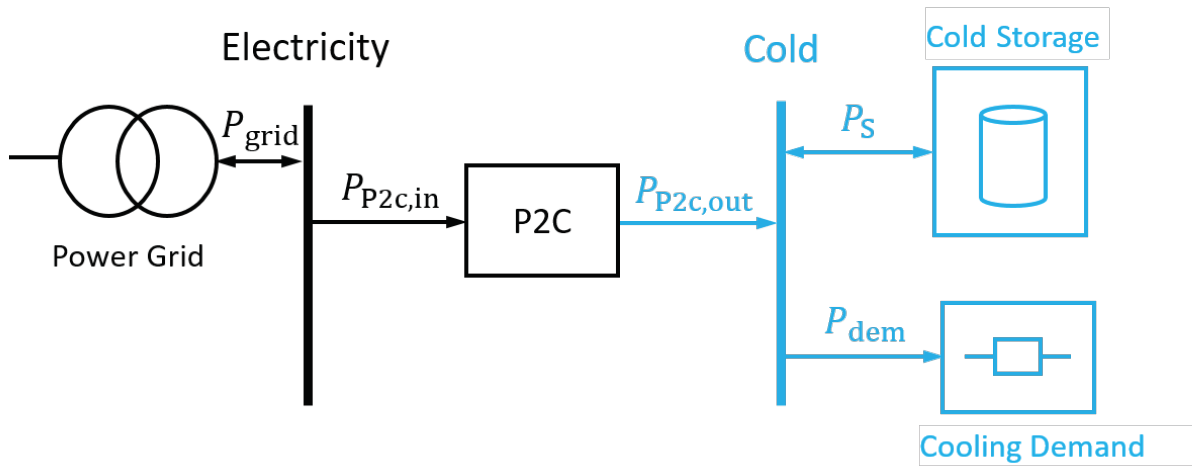
The following analysis uses a simple sector-coupled energy system to show the method’s idea and the reserve storage’s potential. The case study is based on an actual application in the form of an office campus. The system structure is sketched in Figure 2. It needs to fulfill a specific demand for cooling for a consumer. Therefore, a power-to-cold plant is used, realized by a compression refrigeration machine, in the following power-to-cold plant. It is fed with electricity from a public grid. Additionally, a thermal energy storage system for the cold demand is assumed.
We describe the system using model equations for each component and the coupling points. For simplicity and to illustrate principal effects, linear models with constant efficiencies and neglecting self-discharge are considered. The governing equations describing the model are presented and explained for all relevant system components.

2.1.4. Power-to-Cold Plant

The power-to-cold plant converts electric power P P 2 c , in el into thermal power P P 2 c , out th , i.e.,
P P 2 c , in el = P P 2 c , out th / η P 2 C ,
where η P 2 C is a constant coefficient of performance of the plant. Since the power-to-cold plant can only consume power and refeeding into the grid is physically not possible, the following equation holds:
0 P P 2 c , in el .
Additionally, the operation range of the plant is limited by the maximum installed power P P 2 c , out max :
0 P P 2 c , out P P 2 c , out max .

2.1.5. Energy Storage System

The power-to-cold system is coupled with a thermal energy storage system. This results in the following energy balance in discretized form:
E s ( t k ) = E s ( t k 1 ) + η E P s , char th ( t k ) · Δ t 1 η E P s , dis th ( t k ) · Δ t ,
where E s ( t k ) is the stored energy at a specific point in time t k , η E is the charge and discharge efficiency, and P s , char th and P s , dis th are the charge and discharge power, respectively. We assume the initial value of E s to be zero since the storage system only comes into play when appropriate price signals are received. Again, the operation range of the storage system is limited to the maximum charging and discharging power P s max :
0 P s , char th P s max ,
0 P s , dis th P s max ,
and the capacity of the energy storage system is limited by the energy capacity E s max :
0 E s E s max .

2.1.6. Power Balances

Each form of power must be balanced. For the electricity, it holds
0 = P grid el P P 2 c , in el .
The realized electricity supply from the grid P grid el is the sum of purchased power at the two markets. For the cold balance, it yields
P dem = P P 2 c , out th + P s , dis th P s , char th .
Therefore, P dem is the cooling demand of the customer that needs to be provided by the energy system.

2.2. Scheduling and Trading

2.2.1. Day-Ahead Market

As described in Section 2.1, the electricity is purchased at the day-ahead market based on the load forecast. We want to evaluate the influence of the reserve capacity and not focus on different bidding strategies. Therefore, we assume an optimal energy purchase and schedule for the components. The resulting optimization problem is defined as follows:
min P grid , DA el , P s , dis th , P s , char th k = 1 n C e , DA ( t k ) · P grid , DA el ( t k ) · Δ t ,
with Δ t = t k t k 1 . The objective function is the cost of purchasing energy from the grid over the evaluated period. Here, C e , DA describes the time-dependent price signals at the day-ahead market, and P grid , DA · Δ t the corresponding purchased energy. The model equations, Equations (1)–(9), are also considered as equality and inequality constraints. However, in (9), only the forecast for the demand P for can be taken into account.

2.2.2. Intraday Market

The second step of the operation is to compensate for deviations in the load forecast with the help of the reserve storage or by compensation trades at the day-ahead market. As mentioned before, we assume a rule-based approach since upcoming loads are known only on a short-term basis. Table 1 summarizes the control rules for the traded power P grid , ID el and the charge and discharge power of the storage system. They depend on the differences Δ P between the forecast P for and the actual demand P dem ,
Δ P = P dem P for ,
as well as the current price at the intraday market C e , ID . The combinations result in nine cases (c.f. Table 1). The columns represent the additional and reduced demand and the case where the demand equals the forecast. The rows differentiate whether the current energy price at the intraday market is below a maximum purchase price C e lim , above a minimum price for sale C e lim + , or within these limits. Within these rules, the following help variables are used. The set point for the maximum possible discharge and charge power can be limited either by the energy content of the storage system or by the maximum charge and discharge power, respectively,
P s , dis set = min E s · η E Δ t , P s max
and
P s , char set = min E s max E s η E · Δ t , P s max .
The given system design makes it physically impossible to feed stored thermal energy into the electricity grid. Therefore, energy can only be sold by offering energy purchased at the day-ahead market over the same period. Therefore, the maximum amount of energy that can be sold at any time is limited by
P sell max ( t ) = P grid , DA el ( t ) .

2.3. Evaluation

In the analysis, we vary the share of the reserve storage to find an optimal trade-off between flexibility at the day-ahead market and reserve storage to compensate for deviations in the load forecast. For a fair comparison, the total electricity costs at the day-ahead and intraday markets are summed up and compared with the system without reserve storage, i.e.,
C p , tot = k = 1 n C e , DA ( t k ) · P grid , DA ( t k ) · Δ t + k = 1 n C e , ID ( t k ) · P grid , ID ( t k ) · Δ t .

2.4. Definition of Forecast Quality

The optimal reserve storage share depends on the load forecast quality. For a perfect forecast, no reserve storage is necessary, and in case of significant deviations, it is assumed that higher reserve shares could be beneficial. Different definitions of forecast quality can be chosen, where the most straightforward approach might be the use of the mean difference between the load forecast and the actual demand. Another method would be using the standard deviation σ over all analyzed time steps of this difference. Even though these approaches might work to characterize load curves with similar mean values, comparing load cycles with a larger variation of those is not suitable. Other more advanced ways to define forecast quality might be, for example, the use of robust measures of scale. However, to keep focus on the topic of this article in the present analysis, we took a slightly adapted form of the coefficient of variation f CV to quantify forecast quality. It is defined by the standard deviation between the load forecast P for and the realized demand P dem normed to the mean value μ of the demand P dem :
f CV = σ | P dem P for | μ ( P dem ) .
This index is easy to evaluate and can be adapted to other cases.

3. Results for Generated Case Study

In this chapter, the input data for the investigated case study is first described and then analyzed concerning different aspects. The last part of this section discusses the influence of plant dimensioning.

3.1. Definition of Case Study

The case study is defined by the plant configuration and dimensioning of the plants that must be operated. These parameters are given in Table 2. They are adapted from the implemented system.
Furthermore, price signals for the investigated markets, load curves, and forecast time series need to be fixed for the evaluation. These will be discussed in the following.
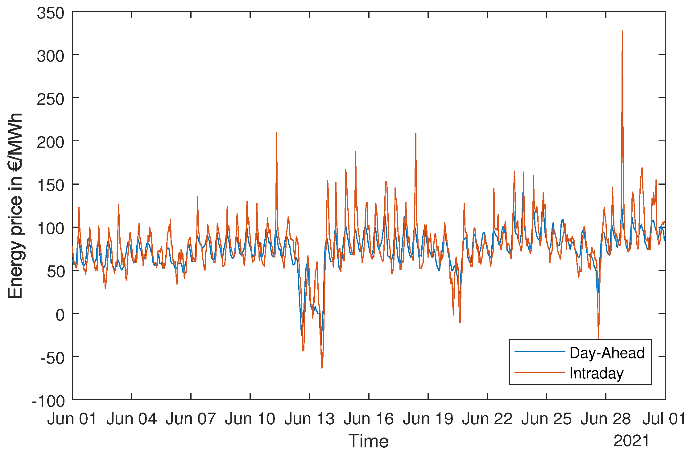
The present study considers the day-ahead market for electricity purchasing and the intraday market for short-term compensation of differences. At the day-ahead market, bids from suppliers and consumers are collected until noon of the day before fulfillment. Subsequently, the EPEX Spot energy exchange awards the respective bids. A demand not covered by the day-ahead market, e.g., due to short-term changes in the anticipated load or due to deviating generation from renewable energies, can be covered by continuous intraday trading up to 5 min before delivery. The price determination takes place individually between the trading partners [13]. For the present analysis, the price data from October 2020 to October 2021 is taken from Bundesnetzagentur [27] for the day-ahead market and internal data for the realized intraday trading. Figure 3 shows an example of the time series of the prices for June 2021.
For the present analysis, we need different load curves and prognoses with different qualities, which we want to vary systematically. Since only limited data are available, we choose to generate different load curves with a given characteristic and vary the introduced coefficient of variation while keeping the mean value of the load curves constant.
The load curves employed are simulated by steady-state, Gaussian stochastic processes modeled by the spectral representation method based on the work conducted by Shinozuka and Deodatis [28]. For this purpose, a given load curve P dem 0 ( t j ) in discrete time t j with j = 0 , , N 1 , where N is the data set size, is first decomposed into its frequency spectrum using the discrete Fourier transform to extract its characteristics, i.e.,
S n = j = 0 N 1 P dem 0 ( t j ) · e i n ω 0 j ,
where ω 0 = 2 π / N and i is the imaginary unit. From the two-sided spectrum conserved in this way, a new random load curve can be simulated using the spectral representation
P ˜ dem ( k ) ( t ) = 2 n = 0 N 1 A n cos ω n t Φ n ( k ) ;
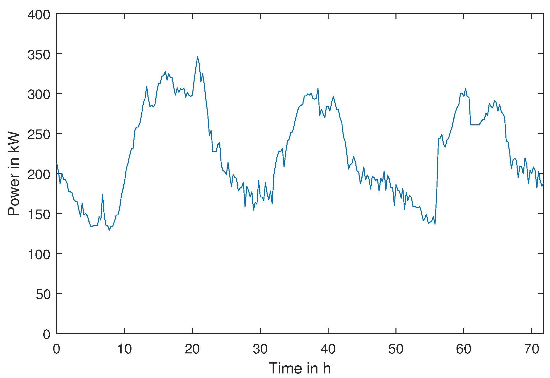
see Equation (35) in [28] for details. P ˜ dem ( k ) ( t ) is the k-th realization of the stochastic process P dem ( t ) , which represents the realized demand. The simulated load curves are based on a load curve P dem 0 ( t j ) recorded over 3 days at a power-to-cold plant in an office campus, as shown in Figure 4.
By transforming the input signal into the frequency domain and preserving the spectrum, the characteristics of the input signal are preserved. At the same time, any load curve simulated in this way has a random shape due to reverse transformation into the time domain—c.f. Equations (17) and (18). By varying the input signal amplitude using a suitable coefficient, arbitrary load curves with different coefficients of variation can be generated. A parameter study adapted to the plant types investigated in Section 4 provided reasonable values for f CV between 0.3 and 1.
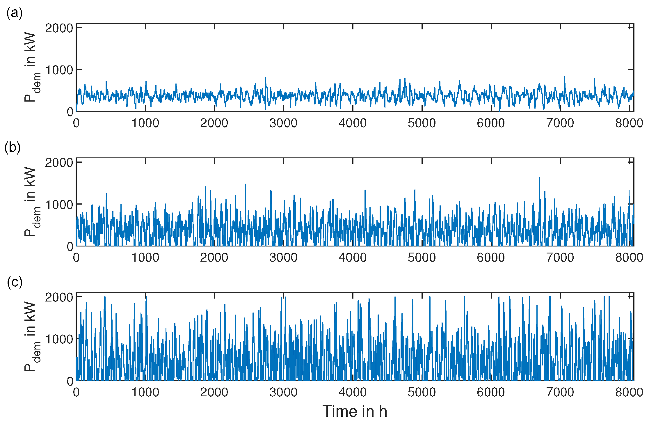
Figure 5 shows three selected examples for the generated load curves resulting in coefficients of variation of (a) 0.3, (b) 0.7, and (c) 1. A larger coefficient of variation leads to larger amplitudes in the load curve, leading to a lower assumed forecast quality.

3.2. Results for Base Case

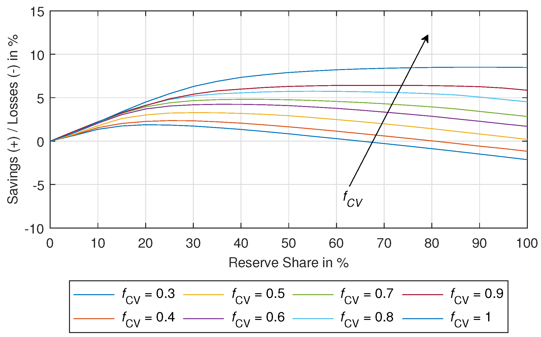
The given case study should investigate under which conditions a storage reservation is beneficial and what share of the storage system should be reserved. Therefore, Figure 6 shows savings or losses of the costs C p , tot for different reserve shares and input signals compared with no reserve storage—c.f. Equation (15). The potential savings are in the order of several percent of the total costs. It is significant, especially if large amounts of electricity must be purchased to operate the system.
The following general trend becomes visible for low coefficients of variation (i.e., a good forecast quality). A reserve share of 10% to 30% is reasonable, and the savings can be generated compared with the case without reserve storage. For larger reserve shares, even losses are possible. The reason is the reduced flexibility at the day-ahead market and consequently more expensive electricity purchasing. The benefits of real-time control cannot compensate for this. For worse forecast quality, this trend is declining, and more benefits can be generated from the reserve storage. For the case with a coefficient of variation of 1, taking the complete storage system as reserve storage is advantageous.
From the results presented, the optimal reserve share was determined as a function of the coefficient of variation. Figure 7 shows that the optimal reserve share is increasing for an increasing coefficient of variation and thus for worse forecasts.

3.3. Variation of Technical Parameters

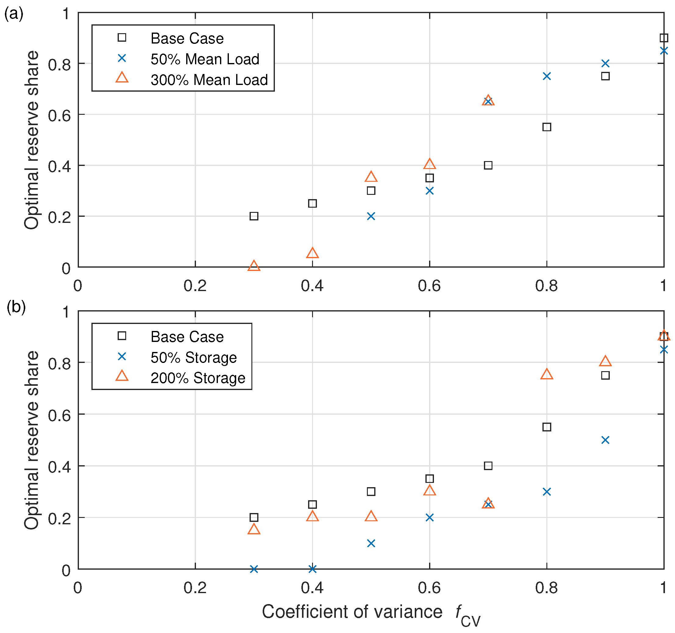
In the base case, we investigated the forecast quality’s influence on the reserve capacity’s optimal share. However, the setup of the system will influence the results. Therefore, in the first step, the arithmetic mean value of the load curve is changed to 50% and 300% of the initial value, whereas the dimension of the power-to-cold plant and the storage system remains as in the base case. Figure 8a shows the optimal reserve share for both in comparison with the base case (black). Due to the power limits of the power-to-cold plant and the used load curve simulation, large coefficients of variation cannot be evaluated for the case with high mean values of the demand (300%).
For all evaluated cases, the found trend is the same: the optimal reserve share increases for increasing f CV . The largest value of f CV also results in the largest optimal reserve share in each case. In both new cases, the optimal reserve share is partly below and partly above the base case value. Thus, a clear trend for the exact numbers cannot be derived, but the qualitative course remains unchanged.
The second aspect to be highlighted is the influence of the storage system size. For this purpose, tests were carried out with lower and higher storage capacities. The storage capacity in the base case was assumed to be 5000 kWh. It corresponds to a minimal charge time of 2.5 h when operating the power-to-cold system at maximum power. In the analysis, it is changed to 50% and 200% of the storage capacity of the base case. This means that the storage system can be fully charged in 1.25 and 5 h, respectively, with unchanged maximum output. Figure 8b shows the optimal reserve share for these compared with the base scenario.
Again, the storage capacity does not change the results qualitatively: the optimal reserve share increases with an increasing coefficient of variation f CV . The trend in the scenario with a large storage capacity in the f CV = 0.7 range is unclear. Since this represents an individual case, we assume that it results from special correlations of price and demand. For reduced storage capacities, the optimal reserve share is lower than in the base case. On the other hand, the case of increased storage capacity needs to be clarified. Here, deviations of up to f CV = 0.7 result in a lower optimum reserve share than in the base case, and for larger values, the optimum reserve share is more prominent than in the base case.
The variation of the technical parameters shows a general correlation between the selected uncertainty measure f CV and the optimal reserve share in the sense that in nearly all cases, larger values of f CV lead to a larger optimal reserve share. However, a direct correlation or scalability of the optimal reserve share with the mean value of the load or the storage system size could not be determined. Nevertheless, these examples show that keeping a significant reserve in case of greater uncertainty does make sense. The actual storage capacity seems to play a rather subordinate role here. A general recommendation for the reserve share based only on the uncertainty factor f CV was not possible since correlations between price signal and demand significantly impact overall results. Nevertheless, some recommendations for the reserve share as a function of the coefficient of variation can be derived from the present results. From a coefficient of variation of around 0.75–0.9, setting the reserve share to half or even more of the storage capacity is recommendable.

4. Results with Measured Data

The last aspect of the present analysis is comparing the discussed results based on generated load curves (Section 3) with measured data. With this, we want to verify the algorithm’s applicability to real cases. The analysis performed in this section is based on the load data recorded at the EUREF campus within the project “WindNODE”. Additionally, the plant operator provided three load forecasts generated by different machine learning algorithms. Complete data sets are available for June to September 2021.
In the following, the analysis’s input signals are introduced and then evaluated and discussed.

4.1. Input Signals

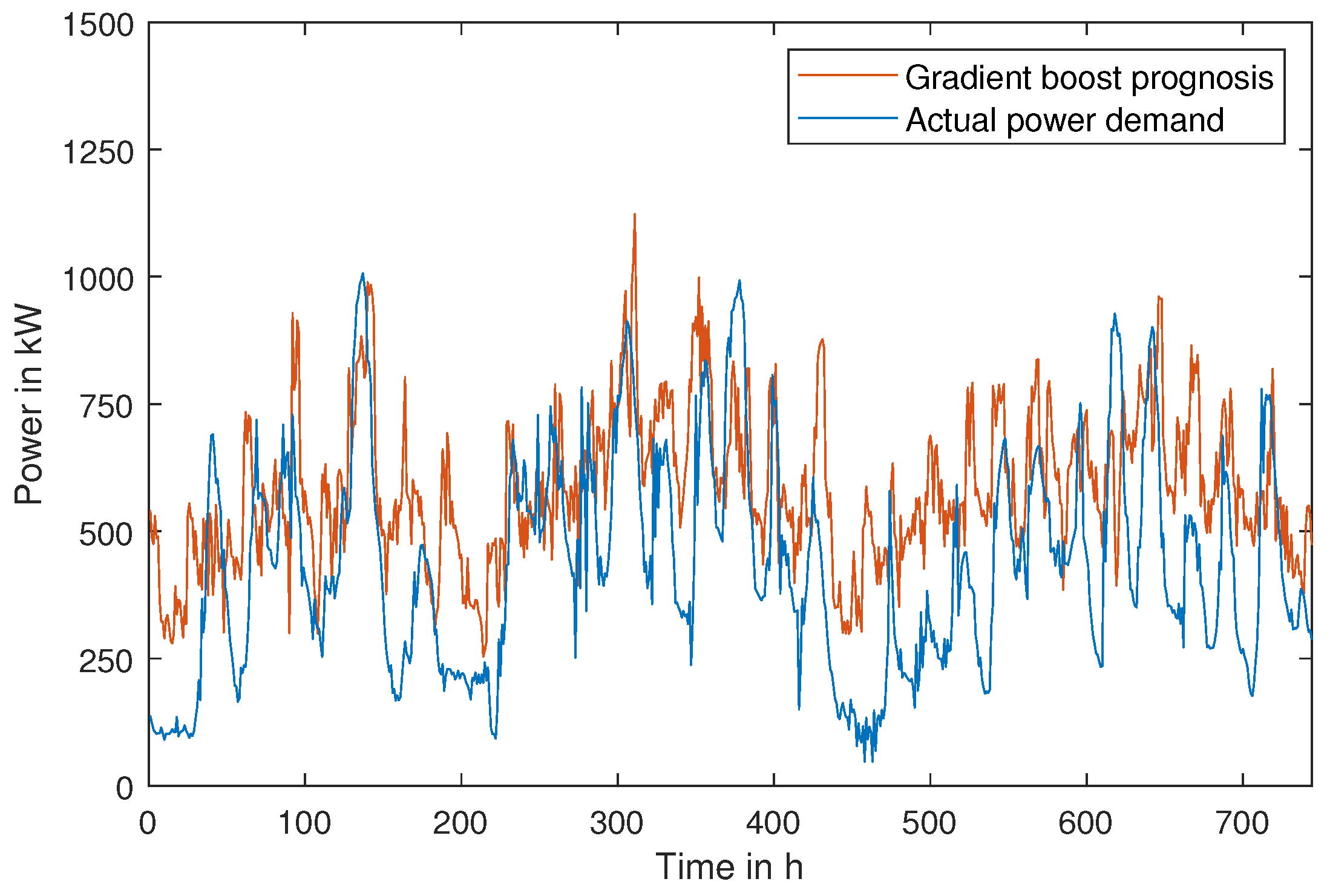
The load data were recorded at a real energy plant site [13,18]. The load forecasts were created by [18] using machine learning methods implemented in the Python module Scikit-learn, which integrates a wide range of machine learning algorithms and is distributed under the simplified BSD license [29]. The data have an hourly resolution and the features weekday, differentiation weekday/weekend, load curve, and outdoor temperatures (c.f. [18]). The outdoor temperatures were obtained from http://openweathermap.org (acssessed on 1 October 2021) for the corresponding longitude and latitude of the site in hourly resolution. The training was performed with approximately 1 year of data (1 October 2020 to 1 September 2021 training data, 1 September 2021 to 11 October 2021 test data) with the methods gradient boost regression [29,30], XGBoost [31], and random forest regression [32]—several methods were tried by [18], and the chosen ones delivered the best results. Figure 9 shows the measured load demand and the prognosis by the gradient boost method.
This study takes the recorded price signals for the day-ahead and the intraday market for the corresponding times.

4.2. Results

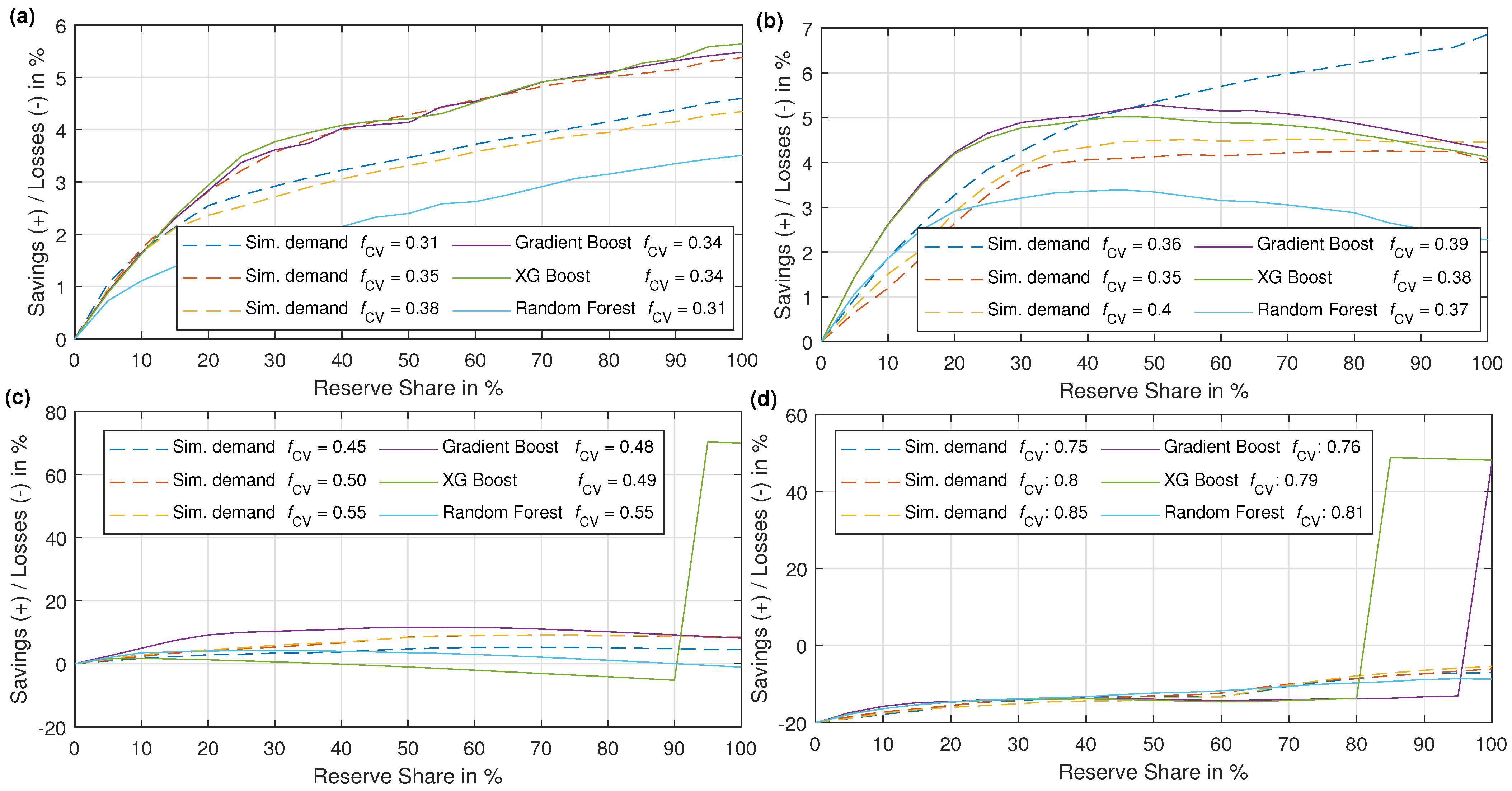
The machine learning forecasts are evaluated with the approach and the scheduling rules described in Section 2. They are compared with the results for generated load curves analyzed with the approach of the base case study (c.f. Section 3). The mean values and the coefficient of variation of the measured data and the forecast are used for good comparability. Figure 10 shows the achieved savings or losses over the respective reserve share for the measured load curves and the respective generated data sets for the investigated months.
A differentiated picture emerges over the 4 months investigated. While the qualitative improvements in the results of the measured load data in Figure 10a for June 2021 are very similar to the improvements in the generated load data, there are deviations in Figure 10b for July 2021. In the case of the measured data, the most significant improvements in results are achieved in the range of 40–50% reserve share. In contrast, in the case of the generated load curves, the storage system should be used entirely for the reserve (reserve share of 100%).
In August and September 2021 (Figure 10c,d), the analysis with the forecast methods XGBoost and gradient boost show a noncontinuous course with high savings at large reserve shares. We assume that this phenomenon is caused by the correlation of exceptional price and demand signals at certain times. Therefore, we consider this result to be unrepresentative. Besides this outlier, in August, the optimal reserve share for the measured profiles is at low and medium values (25% for random forest and 55% for gradient boost). At the same time, the most considerable improvement in results for all three generated load curves was obtained at a reserve share of 70%. In September 2021, again disregarding the outliers, the generated and measured load data trajectories resemble each other. Thus, in all cases, the maximum improvements in results are obtained at very high reserve shares of 85% to 100%.
The comparison of the available measured and generated load data allows for two conclusions. On the one hand, the algorithm developed is suitable for achieving improvements in results even under real conditions. On the other hand, it is not easy to make general recommendations for suitable reserve shares based on the available data since the ratio of the price signals also has a significant influence in addition to the forecast inaccuracy. Therefore, the evaluation should be carried out for short periods to obtain the best possible recommendation for selecting a reserve storage share.

5. Conclusions and Outlook

The present paper shows a concept to handle uncertain load forecasts by reserving a share of the available energy storage system for short-term balancing. Due to the reservation of a particular share of the energy storage system, the flexibility at the day-ahead market is limited, with the benefit of more flexibility at the short-term intraday trading market. To show the effects, we analyzed a simple sector-coupled energy system. It is based on a real example system for cooling an office campus with the help of a power-to-cold plant.
With the help of the case study, we showed that it is economically reasonable to reserve a particular share of the energy storage system. Additionally, we quantify the benefit by up to 10% of the energy costs for the given setting, which can be saved with an optimal reserve share. This effect was shown systematically with generated data and verified with measured data from the EUREF campus to show the real potential. The concrete value of the optimal share depends not only on the forecast quality but also on the dimensioning of the components. Furthermore, some exceptional cases regarding the price signals and the load curves yielded different results. Therefore, we did not find a scalability rule for this, and a general recommendation for reserve share is impossible. However, the qualitative trend is that a larger reserve share is optimal for increasing uncertainty. For a coefficient of variation of around 0.75–0.9, setting the reserve share to half or even more of the storage capacity is recommendable.
The present study’s results could be further strengthened if additional measurement data are used. Therefore, the different influences and the robustness of the approach could be studied and compared with other approaches, such as model predictive control (MPC)–based operation. Moreover, other plant setups, e.g., with a power-to-heat plant, could give further insights into the suggested approach’s potential.
Overall, the described approach is easier to implement than optimization-based methods and offers cost-saving potential. The operator must regularly compute the optimal reserve share for the available data set for best results.

Author Contributions

Conceptualization, M.R. and A.B.; methodology, M.R., A.B. and C.E.; software and formal analysis, J.K.; resources, R.H.-R.; data curation, J.K.; writing—original draft preparation, A.B. and J.K.; writing—review and editing, J.K., A.B., C.E., M.R. and R.H.-R.; visualization, J.K.; supervision, R.H.-R. All authors have read and agreed to the published version of the manuscript.

Funding

M. Rath acknowledges the support of the German Federal Ministry for Economic Affairs and Climate Action (BMWK) within the WindNODE subproject “Construction, Integration, and Operation of a Power-to-Heat/Cold Plant at the EUREF-Campus with Showcase Function” (grant number 03SIN515), executed by GASAG Solution Plus GmbH, with funding provided as part of the project WindNODE, which is again part of the funding program “Intelligent Energy Showcase––Digital Agenda for the Energy Transition” (SINTEG, grant number 01171449/1).

Data Availability Statement

Some of the data used are subject to the confidentiality of the industrial company involved. However, if required, the author can be contacted so that the data can be made available if possible.

Conflicts of Interest

Author Michael Rath was employed by the company GASAG Solution Plus GmbH. The remaining authors declare that the research was conducted in the absence of any commercial or financial relationships that could be construed as a potential conflict of interest. The funders had no role in the design of the study; in the collection, analyses, or interpretation of data; in the writing of the manuscript; or in the decision to publish the results.

References

  1. García Vera, Y.E.; Dufo-López, R.; Bernal-Agustín, J.L. Energy Management in Microgrids with Renewable Energy Sources: A Literature Review. Appl. Sci. 2019, 9, 3854. [Google Scholar] [CrossRef]
  2. Zia, M.F.; Elbouchikhi, E.; Benbouzid, M. Microgrids energy management systems: A critical review on methods, solutions, and prospects. Appl. Energy 2018, 222, 1033–1055. [Google Scholar] [CrossRef]
  3. Nemati, M.; Braun, M.; Tenbohlen, S. Optimization of unit commitment and economic dispatch in microgrids based on genetic algorithm and mixed integer linear programming. Appl. Energy 2018, 210, 944–963. [Google Scholar] [CrossRef]
  4. Li, Z.; Xu, Y.; Feng, X.; Wu, Q. Optimal Stochastic Deployment of Heterogeneous Energy Storage in a Residential Multienergy Microgrid With Demand-Side Management. IEEE Trans. Ind. Inform. 2021, 17, 991–1004. [Google Scholar] [CrossRef]
  5. Kaya, O.; van der Roest, E.; Vries, D.; Keviczky, T. Hierarchical Model Predictive Control for Energy Management of Power-to-X Systems. In Proceedings of the Smart Grids: Key Enablers of a Green Power System, Piscataway, NJ, USA, 26–28 October 2020; pp. 1094–1098. [Google Scholar] [CrossRef]
  6. Vasilj, J.; Jakus, D.; Sarajcev, P. Robust Nonlinear Economic MPC Based Management of a Multi Energy Microgrid. IEEE Trans. Energy Convers. 2021, 36, 1528–1536. [Google Scholar] [CrossRef]
  7. Zhao, Z.; Guo, J.; Luo, X.; Lai, C.S.; Yang, P.; Lai, L.L.; Li, P.; Guerrero, J.M.; Shahidehpour, M. Distributed Robust Model Predictive Control-Based Energy Management Strategy for Islanded Multi-Microgrids Considering Uncertainty. IEEE Trans. Smart Grid 2022, 13, 2107–2120. [Google Scholar] [CrossRef]
  8. Carli, R.; Cavone, G.; Pippia, T.; de Schutter, B.; Dotoli, M. A Robust MPC Energy Scheduling Strategy for Multi-Carrier Microgrids. In Proceedings of the 2020 IEEE 16th International Conference on Automation Science and Engineering (CASE), IEEE, Hong Kong, China, 20–21 August 2020; pp. 152–158. [Google Scholar] [CrossRef]
  9. Kneiske, T.M. Reducing CO2 Emissions for PV-CHP Hybrid Systems by Using a Hierarchical Control Algorithm. Energies 2023, 16, 6176. [Google Scholar] [CrossRef]
  10. Wang, Y.; Dong, W.; Yang, Q. Multi-stage optimal energy management of multi-energy microgrid in deregulated electricity markets. Appl. Energy 2022, 310, 118528. [Google Scholar] [CrossRef]
  11. Scattolini, R. Architectures for distributed and hierarchical Model Predictive Control—A review. J. Process Control 2009, 19, 723–731. [Google Scholar] [CrossRef]
  12. Ejeh, J.O.; Roberts, D.; Brown, S.F. A flexible energy storage dispatch strategy for day-ahead market trading. Comput. Aided Chem. Eng. 2022, 49, 1957–1962. [Google Scholar] [CrossRef]
  13. Beucker, S.; Doderer, H.; Funke, A.; Koch, C.; Kondziella, H.; Hartung, J.; Maeding, S.; Medert, H.; Meyer-Braune, G.; Rath, M.; et al. Flexibility, Markets and Regulation: Insights from the WindNODE Reality Lab. Available online: https://www.windnode.de/fileadmin/Daten/Downloads/FMR_eng.pdf (accessed on 31 January 2024).
  14. Zhuang, H.; Tang, Z.; Zhang, J. Two-Stage Energy Management for Energy Storage System by Using Stochastic Model Predictive Control Approach. Front. Energy Res. 2021, 9, 803615. [Google Scholar] [CrossRef]
  15. Tanja, M. Kneiske and Martin Braun Flexibility potentials of a combined use of heat storages and batteries in PV-CHP hybrid systems. Energy Procedia 2017, 135, 482–495. [Google Scholar] [CrossRef]
  16. Bischi, A.; Taccari, L.; Martelli, E.; Amaldi, E.; Manzolini, G.; Silva, P.; Campanari, S.; Macchi, E. A detailed MILP optimization model for combined cooling, heat and power system operation planning. Energy 2014, 74, 12–26. [Google Scholar] [CrossRef]
  17. Molina, D.; Lu, C.; Sherman, V.; Harley, R.G. Model Predictive and Genetic Algorithm-Based Optimization of Residential Temperature Control in the Presence of Time-Varying Electricity Prices. IEEE Trans. Ind. Appl. 2013, 49, 1137–1145. [Google Scholar] [CrossRef]
  18. Rath, M.; Ray, H.; van Treek, M.; Meeder, A. Untersuchung verschiedener Lastprognoseverfahren für die prognosebasierte Steuerung dezentraler Energieanlagen. BauSim Conf. 2022, 9. [Google Scholar] [CrossRef]
  19. Zhang, Q.; Grossmann, I.E.; Heuberger, C.F.; Sundaramoorthy, A.; Pinto, J.M. Air separation with cryogenic energy storage: Optimal scheduling considering electric energy and reserve markets. AIChE J. 2015, 61, 1547–1558. [Google Scholar] [CrossRef]
  20. Schäfer, P.; Caspari, A.; Mhamdi, A.; Mitsos, A. Economic nonlinear model predictive control using hybrid mechanistic data-driven models for optimal operation in real-time electricity markets: In-silico application to air separation processes. J. Process Control 2019, 84, 171–181. [Google Scholar] [CrossRef]
  21. Chen, J.; Garcia, H.E. Economic optimization of operations for hybrid energy systems under variable markets. Appl. Energy 2016, 177, 11–24. [Google Scholar] [CrossRef]
  22. Yin, W.; Liu, H.; Ni, X.; Zhou, H.; Hou, Y. A Two-stage Rolling Scheduling Strategy for Battery Energy Storage in Multi-periods Electricity Market. In Proceedings of the 2018 IEEE Power & Energy Society General Meeting (PESGM), Portland, OR, USA, 5–10 August 2018; pp. 1–5. [Google Scholar] [CrossRef]
  23. Xu, J.; Chen, Z.; Hao, T.; Zhu, S.; Tang, Y.; Liu, H. Optimal Intraday Rolling Operation Strategy of Integrated Energy System with Multi-Storage. In Proceedings of the 2018 2nd IEEE Conference on Energy Internet and Energy System Integration (EI2), Beijing, China, 20–22 October 2018; pp. 1–5. [Google Scholar] [CrossRef]
  24. Ji, Y.; Xu, Q.; Zhao, J.; Yang, Y.; Sun, L. Day-ahead and intra-day optimization for energy and reserve scheduling under wind uncertainty and generation outages. Electr. Power Syst. Res. 2021, 195, 107133. [Google Scholar] [CrossRef]
  25. Abdeltawab, H.; Mohamed, Y.A.-R.I. Energy Storage Planning for Profitability Maximization by Power Trading and Ancillary Services Participation. IEEE Syst. J. 2022, 16, 1909–1920. [Google Scholar] [CrossRef]
  26. Nguyen Duc, H.; Nguyen Hong, N. Optimal Reserve and Energy Scheduling for a Virtual Power Plant Considering Reserve Activation Probability. Appl. Sci. 2021, 11, 9717. [Google Scholar] [CrossRef]
  27. Bundesnetzagentur. SMARD|Marktdaten. Available online: https://www.smard.de/en/downloadcenter/download-market-data/ (accessed on 1 October 2021).
  28. Shinozuka, M.; Deodatis, G. Simulation of Stochastic Processes by Spectral Representation. Appl. Mech. Rev. 1991, 44, 191–204. [Google Scholar] [CrossRef]
  29. Pedregosa, F.; Varoquaux, G.; Gramfort, A.; Michel, V.; Thirion, B.; Grisel, O.; Blondel, M.; Prettenhofer, P.; Weiss, R.; Dubourg, V. Scikit-learn: Machine Learning in Python. J. Mach. Learn. Res. 2012, 12, 2825–2830. [Google Scholar]
  30. Hastie, T.; Tibshirani, R.; Friedman, J. The Elements of Statistical Learning; Springer: New York, NY, USA, 2009. [Google Scholar] [CrossRef]
  31. Chen, T.; Guestrin, C. XGBoost: A Scalable Tree Boosting System. In Proceedings of the 22nd ACM SIGKDD International Conference on Knowledge Discovery and Data Mining, San Francisco, CA, USA, 13–17 August 2016; Krishnapuram, B., Shah, M., Smola, A., Aggarwal, C., Shen, D., Rastogi, R., Eds.; ACM: New York, NY, USA, 2016; pp. 785–794. [Google Scholar] [CrossRef]
  32. Breiman, L. Random Forests. Mach. Learn. 2001, 45, 5–32. [Google Scholar] [CrossRef]
Figure 1. Sketch for the present approach of two-step, sequential market trades, including forecast errors.
Energies 17 00720 g001
Figure 2. Sketch of the investigated energy system.
Energies 17 00720 g002
Figure 3. Price signals for the June 2021 day-ahead market ( C e , DA , [27]) and intraday trading ( C e , ID , source: internal data).
Energies 17 00720 g003
Figure 4. Load curve recorded from power-to-cold plant (EUREF campus, Berlin).
Energies 17 00720 g004
Figure 5. Selected simulated load curves for different coefficients of variation: (a) 0.3, (b) 0.7, and (c) 1.
Energies 17 00720 g005
Figure 6. Relative effect of keeping reserve storage on energy costs for the base case independent of the reserve share and the forecast quality in terms of coefficient of variation f CV .
Energies 17 00720 g006
Figure 7. Optimal reserve share depending on the coefficient of variation for the base case.
Energies 17 00720 g007
Figure 8. Optimal reserve share depending on the coefficient of variation for (a) changed mean loads and (b) changed storage capacities.
Energies 17 00720 g008
Figure 9. Gradient boost demand forecast compared with the actual power demand for July 2021.
Energies 17 00720 g009
Figure 10. Results of simulated and real demand forecasts for the months of (a) June 2021, (b) July 2021, (c) August 2021, and (d) September 2021.
Energies 17 00720 g010
Table 1. Rule-based operation and trading on the intraday market.
Demand Lower than Forecast Δ P < 0 Demand Equal to Forecast Δ P = 0 Demand Lower than Forecast Δ P > 0
Price lower than maximum buy price
C e < C e lim
Storage empty OR storage (partially) charged:Storage empty OR storage (partially) charged:Storage empty OR storage (partially) charged:
Charge storage as much as possible using excess energy and energy bought at the intraday market. If excess energy cannot be stored completely, sell as much excess energy as possible at the intraday market.Charge storage as much as possible using energy bought at the intraday market.Buy as much energy as possible at the intraday market to meet the demand and charge the storage.
The equations that result from this are
P grid , ID set = min Δ P + P s , char set , P P 2 C max P grid , DA P grid , ID = max P grid , ID set , P sell max P s , dis = 0 P s , char = P grid , ID set Δ P
The equations that result from this are
P grid , ID = max P s , char set , P P 2 C max P grid , DA P s , dis = 0 P s , char = P grid , ID
The equations that result from this are
P grid , ID = max Δ P + P s , char set , P P 2 C max P grid , DA P s , dis = 0 P s , char = min P grid , ID Δ P , P s , char set
Price in range
C e lim C e C e lim +
Storage empty: Sell as much excess energy as possible at the intraday market.Storage empty OR storage (partially) charged: Run the original operation plan as scheduled, no intervention.Storage empty OR storage (partially) charged: Buy energy at the intraday market to meet demand.
Storage (partially) charged: Use as much energy as possible from the storage to meet the demand and sell excess energy at the intraday market.
The equations that result from this are
P grid , ID set = Δ P P grid , ID = max P grid , ID set , P sell max P s , dis = 0
The equations that result from this are
P grid , ID = 0 P s , dis = 0 P s , char = 0
The equations that result from this are
P grid , ID = Δ P P s , dis = 0 P s , char = 0
P s , char = { min Δ P + P grid , ID , P s , char set if P grid , ID > Δ P 0 else
Price higher than minimum sell price
C e > C e lim +
Storage empty: Sell as much excess energy as possible at the intraday market.Storage empty: Run the original schedule, no intervention.Storage empty: Buy energy at the intraday market to meet the demand.
Storage (partially) charged: Use as much energy as possible from the storage to meet the demand and sell excess energy at the intraday market.Storage (partially) charged: Use as much energy as possible from the storage to meet the demand and sell excess energy at the intraday market.Storage (partially) charged: Use as much energy as possible from the storage to meet the demand. If the demand can be fulfilled with storage energy, sell excess energy at the intraday market. If the demand exceeds stored energy, buy energy at the intraday market.
The equations that result from this are
P grid , ID set = Δ P P s , dis set P grid , ID = max P grid , ID set , P sell max P s , dis = 0 if P grid , ID > Δ P P grid , ID Δ P , else
The equations that result from this are
P grid , ID set = P s , dis set P grid , ID = max P grid , ID set , P sell max P s , dis = P grid , ID P s , char = 0
The equations that result from this are
P grid , ID set = min Δ P P s , dis set , P P 2 C max P grid , DA P grid , ID = max P grid , ID set , P sell max P s , dis = min Δ P P grid , ID , P s , dis set P s , char = 0
P s , char = { min Δ P + P grid , ID , P s , char set if P grid , ID > Δ P 0 else
Table 2. Technical parameters of the system for the base case.
ParameterVariableValue
Coefficient of performance η p 2 c 3.67
Rated power of power-to-cold plant P P 2 c , out max 2000 kW
Energy capacity of storage system E s max 5000 kWh
Rated power of storage system (charge and discharge) P s max 500 kW
Storage system efficiency for charge resp. discharge process η E 0.90
Disclaimer/Publisher’s Note: The statements, opinions and data contained in all publications are solely those of the individual author(s) and contributor(s) and not of MDPI and/or the editor(s). MDPI and/or the editor(s) disclaim responsibility for any injury to people or property resulting from any ideas, methods, instructions or products referred to in the content.