
Benchmarking of Various Flexible Soft-Computing Strategies for the Accurate Estimation of Wind Turbine Output Power


Abstract
1. Introduction
2. Materials and Methods
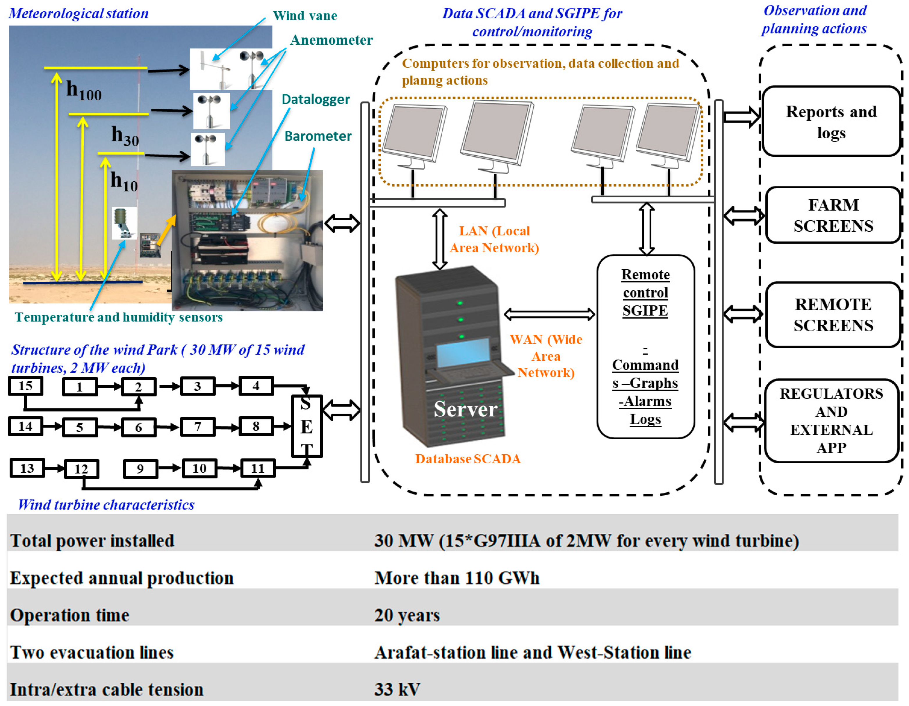
2.1. Collection of the Dataset Used in the Present Computational Analysis
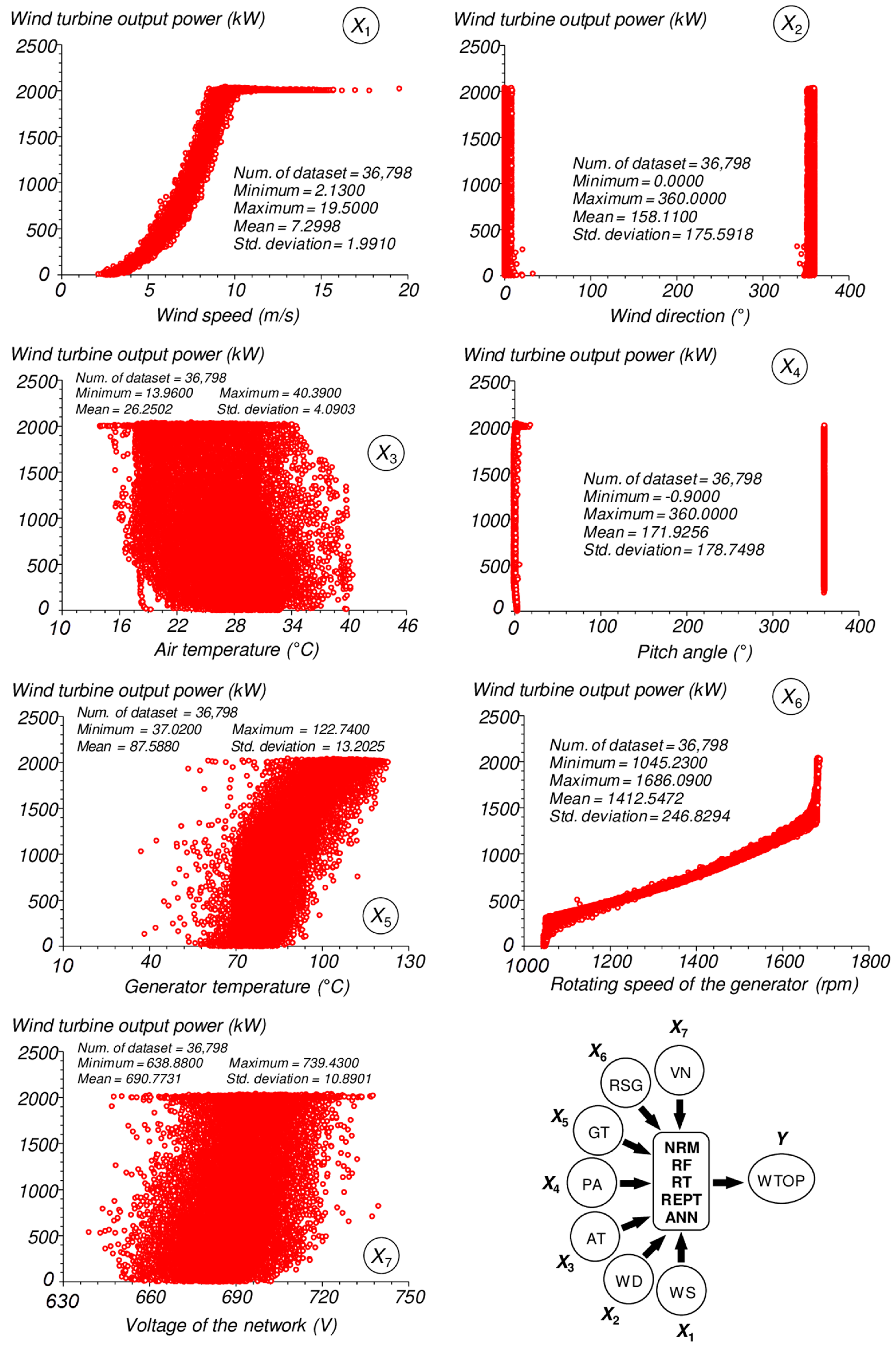
2.2. Importance of Selected Predictor Variables
2.3. Descriptive Statistics of the Model Components Assigned for Training and Testing Phases
2.4. Presentation of Soft-Computing Techniques and Software Systems
2.4.1. Nonlinear Regression-Based Model (NRM)
2.4.2. Random Forest (RF) Model
2.4.3. Random Tree (RT) Model
2.4.4. Reduced Error Pruning Tree (REPT) Model
2.4.5. Artificial Neural Network (ANN) Model
2.5. Description of the Statistical Performance Indices
3. Results
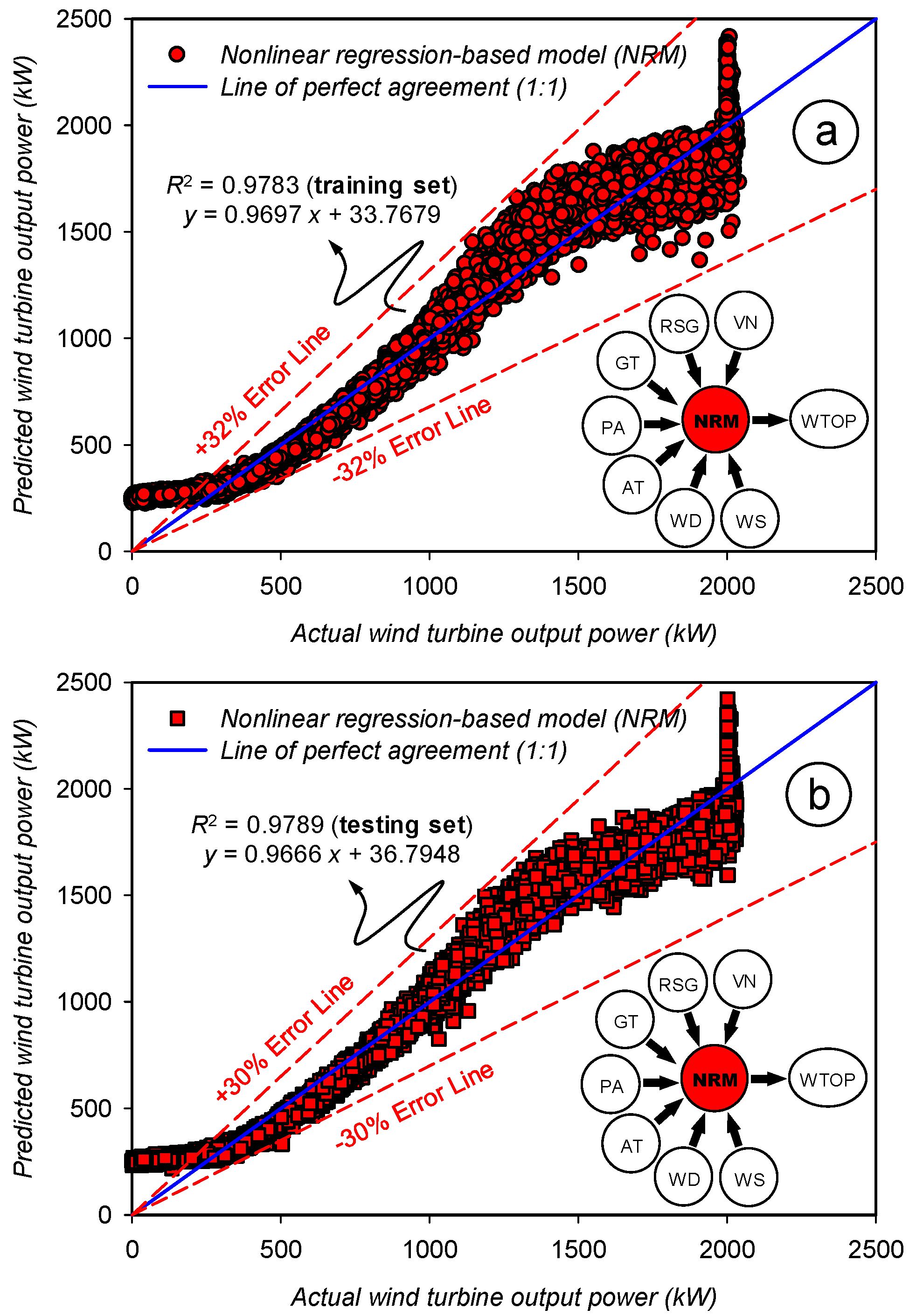
3.1. Assessment of the Prediction Accuracy for the Nonlinear Regression-Based Model
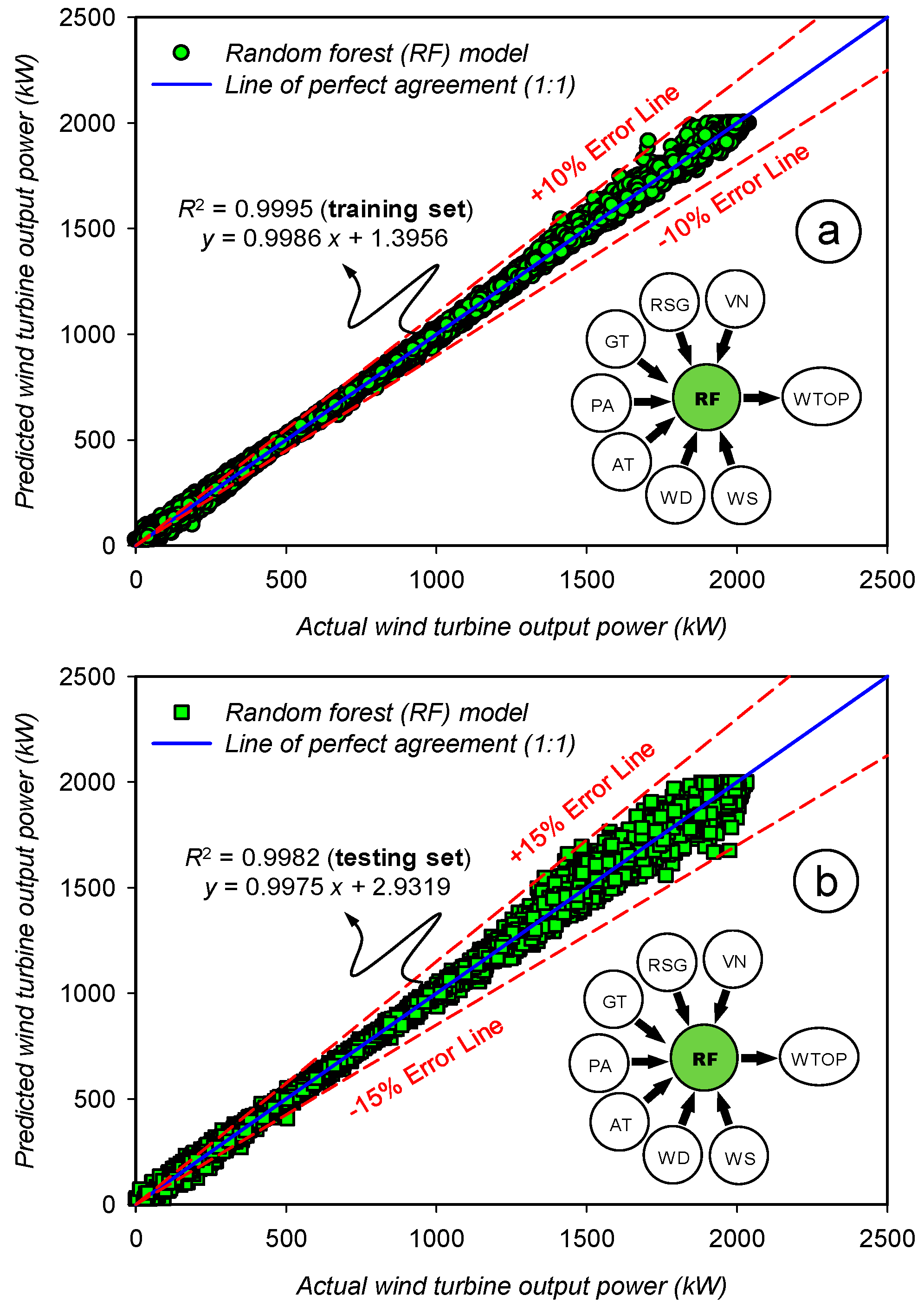
3.2. Assessment of the Prediction Accuracy for the Random Forest (RF) Model
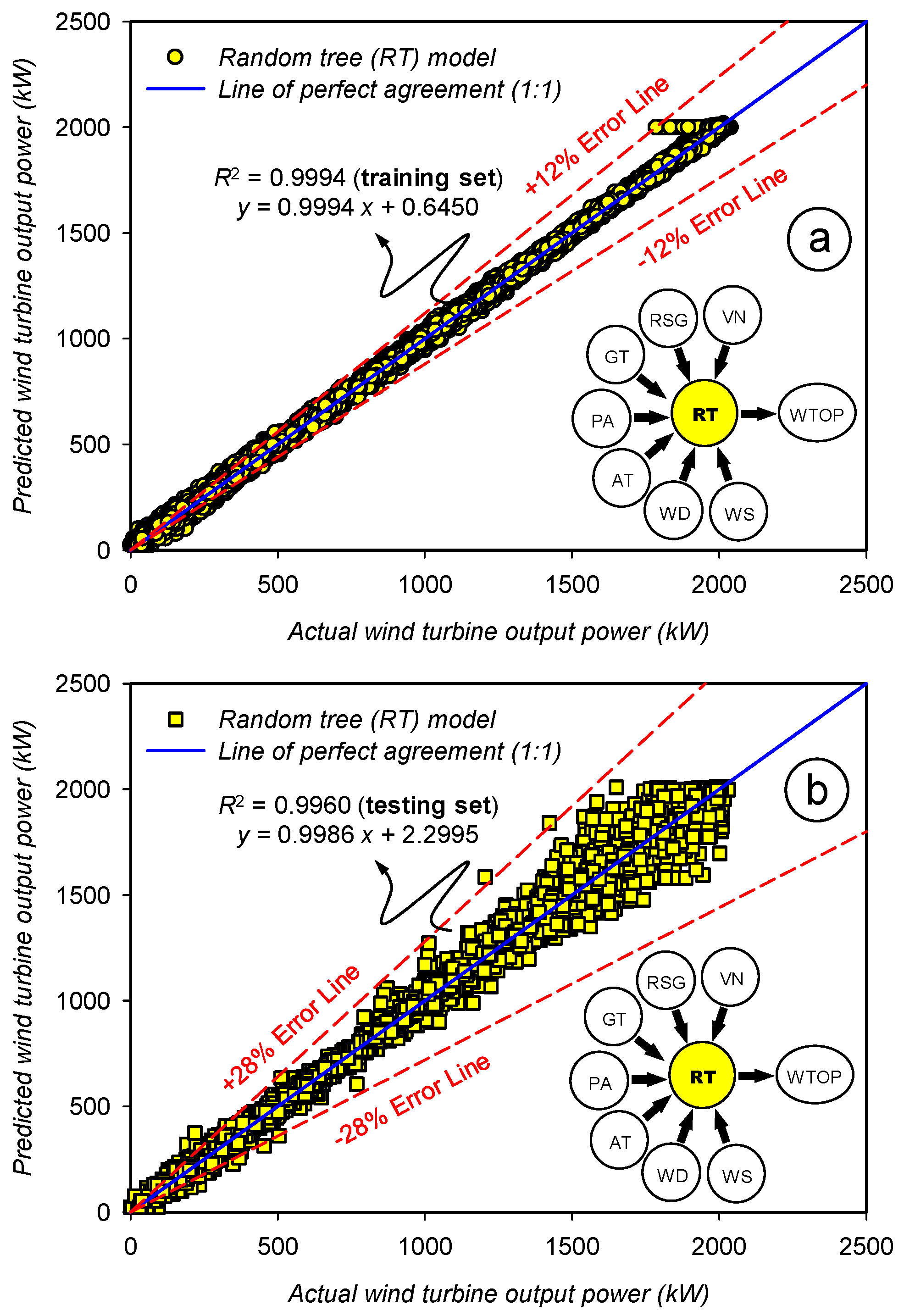
3.3. Assessment of the Prediction Accuracy for the Random Tree (RT) Model
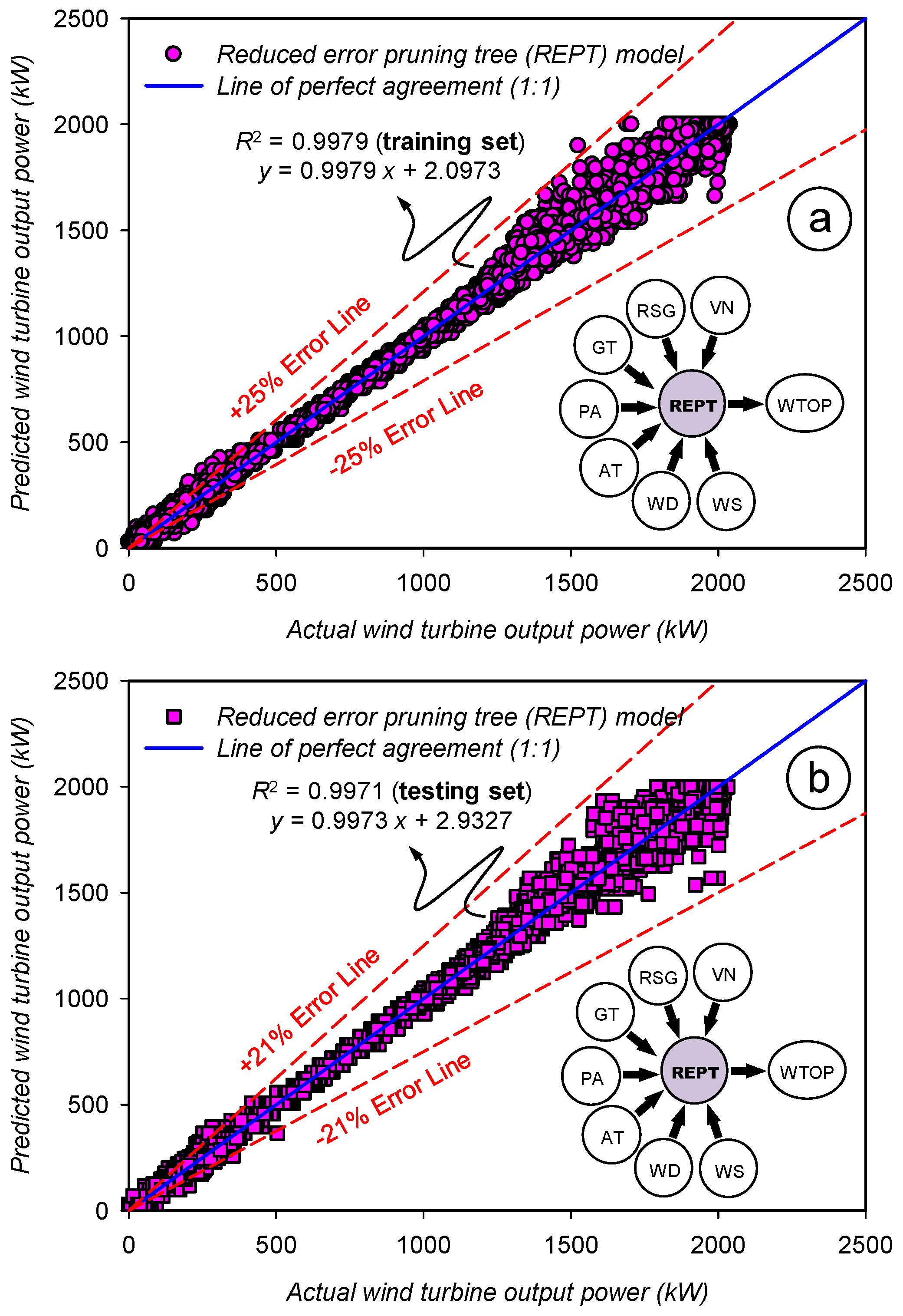
3.4. Assessment of the Prediction Accuracy for the Reduced Error Pruning Tree (REPT) Model
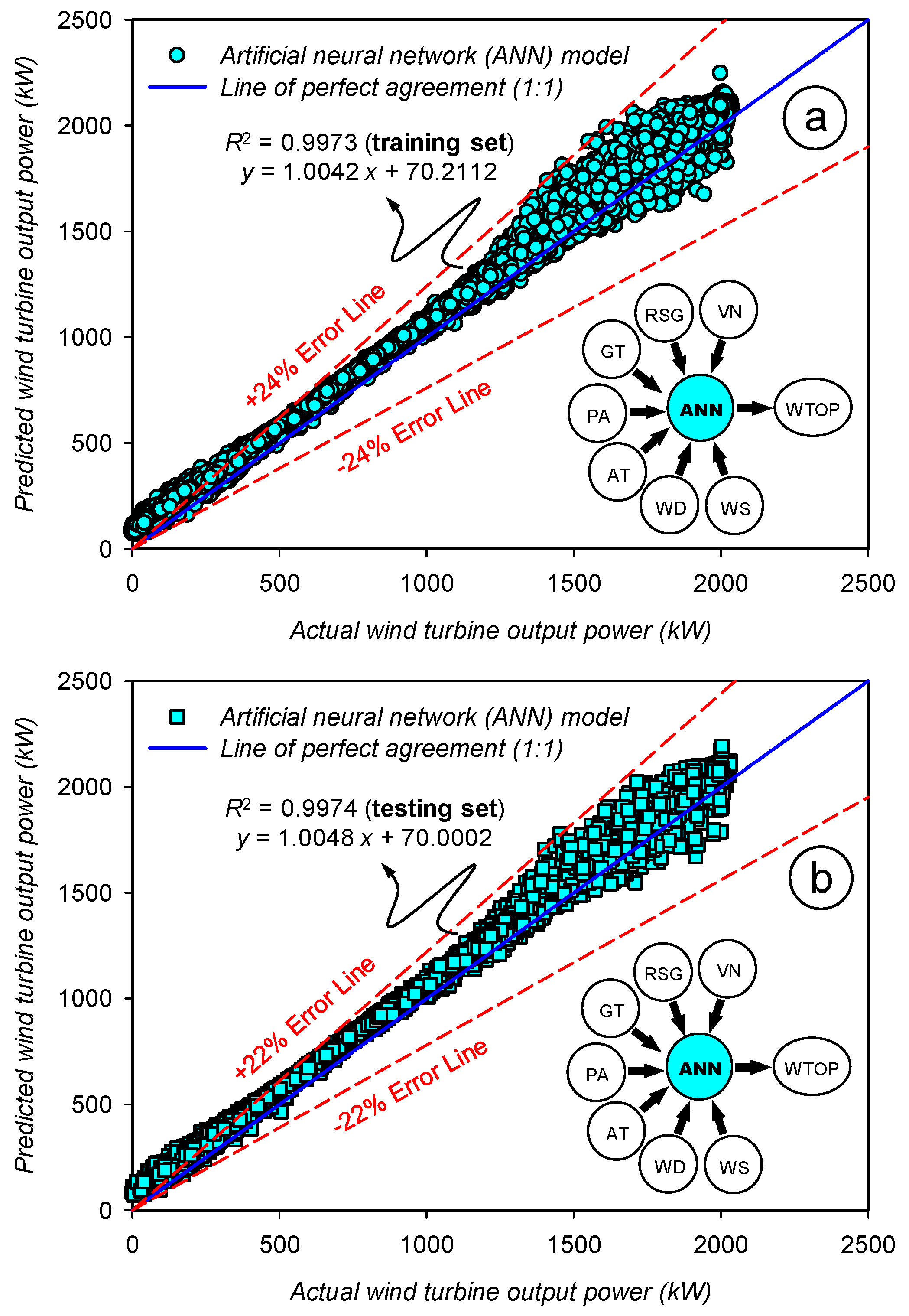
3.5. Assessment of the Prediction Accuracy for the Artificial Neural Network (ANN) Model
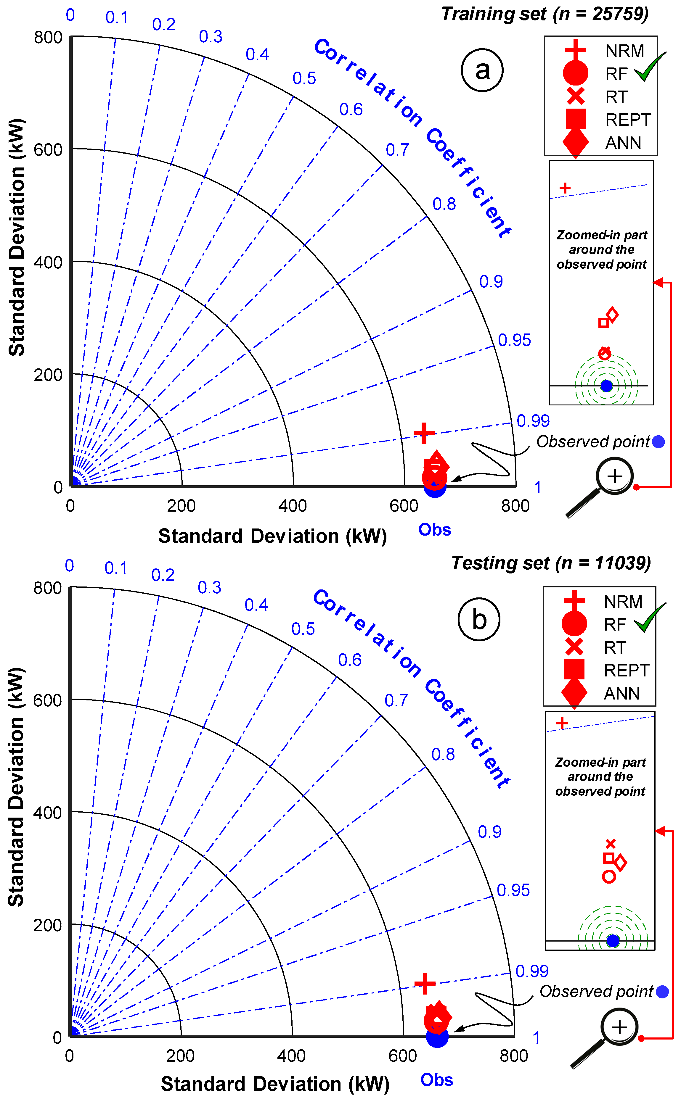
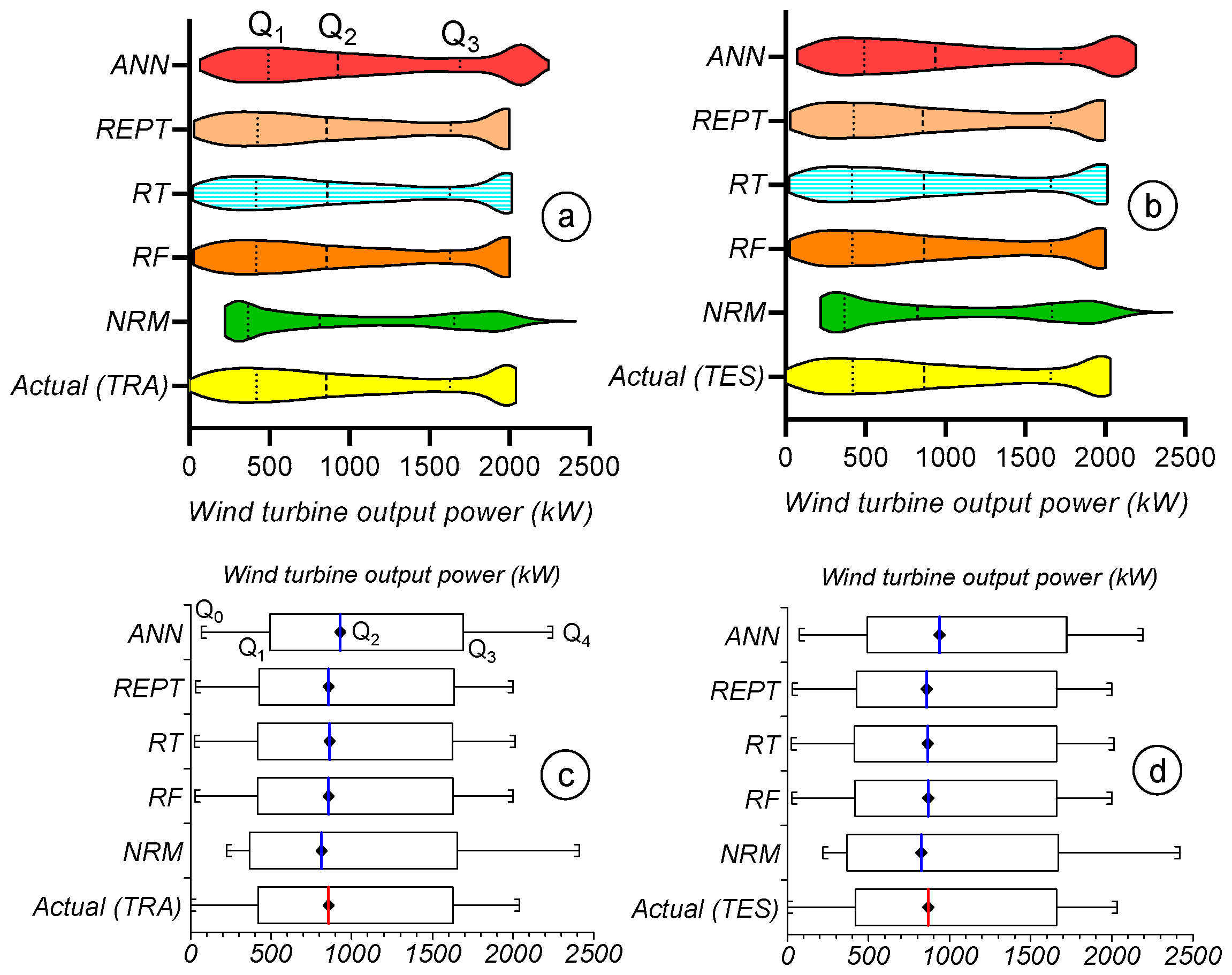
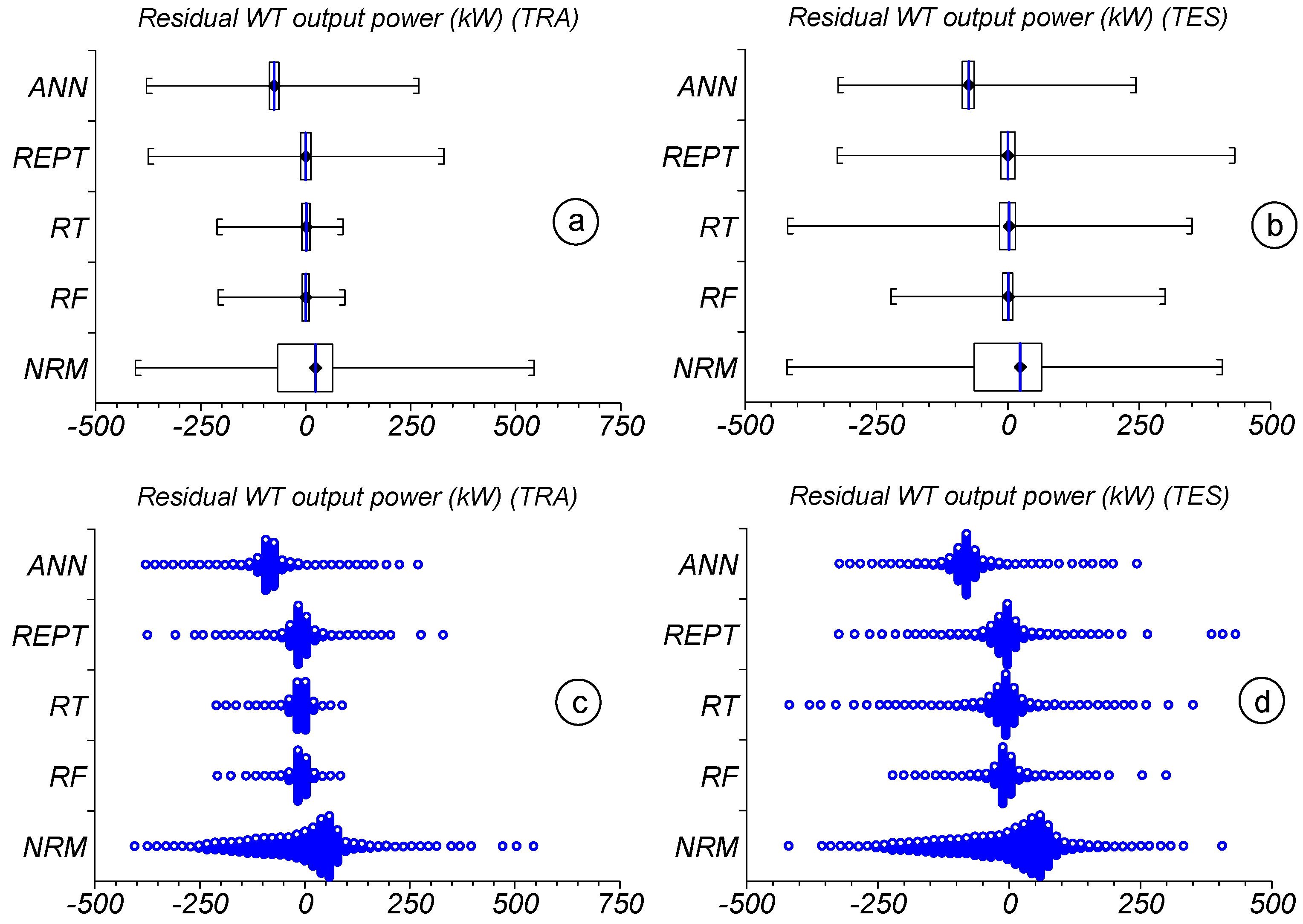
3.6. Inter-Comparison of the Implemented Soft-Computing Models
3.7. Uncertainty Analysis for the Applied Prediction Models
3.8. Sensitivity Analysis for the Best-Fit Soft-Computing Model
4. Discussion
5. Conclusions
Author Contributions
Funding
Data Availability Statement
Acknowledgments
Conflicts of Interest
Appendix A. Data-Intelligent Approaches Used in Wind Speed and WTOP Estimation

| Model Category | Wind Speed Prediction | Study Location | Approach and Methods | Used Datasets | Obtained Performance Metrics | Advantages of Study | Disadvantages of Study |
|---|---|---|---|---|---|---|---|
| Statistical regression method | MSFAE [50] | Xinjiang, China | A novel multi-scale feature adaptive extraction (MSFAE) ensemble model for wind speed forecasting | Three different wind speed time series collected from anemometers are selected to prove the superiority of the model. | Datasite#1 MAPE (%): 3.426 MAE (m/s): 0.146 RMSE (m/s): 0.182 Datasite#2 MAPE (%): 2.312 MAE (m/s): 0.128 RMSE (m/s): 0.166 Datasite#1 MAPE (%): 2.326 MAE (m/s): 0.142 RMSE (m/s):0.186 | The proposed algorithm has the advantages that it provided better global search accuracy and convergence speed than the traditional algorithms |
|
| MKSVRE-WOA [51] | Shandong Province, China | Multi-kernel SVR ensemble (MKSVRE) model based on unified optimization and whale optimization algorithm (WOA) | Wind speed datasets (from 00:00 on 1 September 2011 to 23:50 on 20 September 2011) for two sites (A and B). | Site A MAE (m/s): 0.3698 RMSE (m/s): 0.4786 MAPE (%): 5.21 SAE (m/s): 53.2519 STD (m/s): 0.4796 Site B MAE (m/s): 0.5288 RMSE (m/s): 0.6751 MAPE (%): 8.58 SAE (m/s): 76.1455 STD (m/s): 0.6773 | The model provides results without the need to select a specific kernel function and achieves a global parameter selection. |
| |
| Machine learning | EISM, RTRD Bi-LSTM [14] | Yunnan, China | GWO-CNN-BiLSTM (GCNBiL) networks model with different lengths of convolution operators | Wind speeds collected for 91 days, from 4 January 2010 to 30 June 2010 and included 13,104 sets . | For six-step prediction RMSE (m/s): 0.816 MAPE (%): 13.295 MAE (m/s): 0.635 | The proposed model has greater accuracy than traditional neural network models |
|
| MST-GNN [15] | Denmark, Netherlands | Multidimensional spatial-temporal graph neural networks (MST-GNN) model for wind speed prediction based on multidimensional data | Open-source datasets for wind speed from Denmark and Netherlands | Denmark dataset MAE(m/s): 1.244 MSE (m/s): 2.616 Netherlands Dataset MAE (m/s): 7.849 MSE (m/s): 11.851 | The model performs the best, especially in long-term prediction tasks considering multidimensional data | Model is applied only for wind speed prediction. | |
| MFMS [16] | Zhangjiakou, North China | Method based on multi-feature and multi-scale integrated learning (MFMS) for wind speed prediction | Wind speed data from 16 wind turbines in a wind farm | For 4-h ultra-short-term wind speed prediction MAPE (%): 6.164 RMSE (m/s): 0.275 R2: 0.966 | This method provides a reference for the ultra-short-term wind speed prediction of wind farms. | Model is applied only for wind speed prediction. | |
| CNN-LSM-NDL [17] | Jiangsu Province, China | Hybrid wind speed prediction model based on convolutional neural network and long short-term memory network deep learning model | Historical wind speed dataset collected at two sites from “22 July to 12 August 2017” and from “22 August to 11 September 2017” are used for this study. | Dataset #1 MAE (m/s): 0.1477 RMSE (m/s): 0.1964 MAPE (%): 3.7803 R2: 0.9702 Dataset #2 MAE (m/s): 0.1675 RMSE (m/s): 0.2461 MAPE (%): 2.9065 R2: 0.9726 | Model allows denoising operation in the data preprocessing process, that can provide a high-quality input data, which help to find high prediction performance |
| |
| VMD-TCN-STL [18] | Xinjiang, China | Novel wind-speed prediction model based on variational mode decomposition, temporal convolutional network, and sequential triplet loss | Wind speed series from the SCADA system of the Xinjiang wind farm includes three sets of data are used. | MAPE (%): 4.77 MAE (m/s): 0.11 RMSE (m/s): 0.15 | Prediction accuracy is effectively improved by introducing modal decomposition. VMD exhibits advantages in the same type of method |
| |
| RNN-CNN-LSTM [19] | New Zealand | A novel hybrid neural network scheme based on convolutional neural network (CNN) and long short-term memory (LSTM) | Three datasets given as Data1, Data2, and Data3:
| Data 1 MAE (m/s): 0.4783 RMSE (m/s): 0.6480 R2: 0.9070 Data 2 MAE (m/s): 0.3193 RMSE (m/s): 0.4477 R2: 0.9414 Data 3 MAE (m/s): 0.6281 RMSE (m/s): 0.8724 R2: 0.9775 |
|
| |
| DRIPS-PDI [20] | Nolan and Kern, US | A novel decomposition-recognition-integration-prediction system (DRIPS) based on a newly developed predictive difficulty index | Wind dataset collected for every 10 min for two American sites (Nolan and Kern). | Nolan Site RMSE (m/s): 0.0655 MAPE (m/s): 0.3743 R2: 0.9997 Kern Site RMSE (m/s): 0.0347 MAPE (m/s): 2.4855 R2: 0.9998 | DRIPS associated to (PDI) can provide excellent performance in the accuracy of wind speed prediction and the complexity of the proposed prediction system is acceptable to the industry with the increase in computing power of modern hardware devices |
| |
| CNN-BILSTM-MOHHO [21] | Hebei, China | Variable short wind speed prediction model of Capsule Neural Network (Capsnet) and bidirectional Long-and Short-Term Memory Network (BILSTM) combined with Multi-Object Harris Hawk optimization (MOHHO) | Historical wind speed information from wind farm and multidimensional meteorological variables | Combined model MAE (m/s): 0.1646 MAPE (%):2.43 RMSE (m/s): 0.1992 | The proposed model combines historical data of multiple meteorological data, so the model performs better than other univariate machine learning models. |
| |
| WT-CNN-tSVR [33] |
| Hybrid techniques employing wavelet decomposition transform in tandem with convolutional neural network and twin support vector machine | Wind speed datasets collected in three different periods (three months, 12 months, and 36 months) at the height of 10 m over 10 min | Sotavento (36 months) RMSE (%): 0.275 MSE (m/s): 0.0756 VejaMate (36 months) RMSE (%): 0.1375 MSE (m/s): 0.01890 Madryn (36 months) RMSE (%): 0.085 MSE (m/s): 0.0072 | The model outperforms the classical and simple machine learning for wind speed prediction. |
| |
| Artificial intelligence | EPT-CEEMDAN-TCN [52] | Gansu, Liaoning, Jiangsu, China | A hybrid decomposition method coupling the ensemble patch transform (EPT) and the complete ensemble empirical mode decomposition with adaptive noise (CEEMDAN) | Historical wind speed data from three wind farms located at Gansu, Liaoning, and Jiangsu in China | Gansu site MAE (m/s): 0.28890 RMSE (m/s): 0.40157 MAPE (%):0.07595 Liaoning site MAE (m/s): 0.15659 RMSE (m/s): 0.19586 MAPE (%):0.08896 Jiangsu site MAE (m/s): 0.17790 RMSE (m/s): 0.22361 MAPE (%): 0.09606 | The proposed model has the capability of decomposing the nonlinear volatility completely and allows higher computational efficiency. | Only the wind speeds are considered as input variables to the model. |
| ED-Wavenet-TF [53] | Minnesota, USA | A novel forecasting model called EDWavenet-TF | Two WS datasets collected from wind farms in Nebraska and Minnesota, USA (in 2012 and 2011, respectively) | MAE (m/s): 0.8018 RMSE (m/s): 1.1052 R2: 0.9135 SMAPE (%): 13.9128 | ED-Wavenet-TF outperforms the comparable models in most cases at the 1% significance level and could be used for the wind speed and wind power forecasting. | Only the wind speeds and wind power were considered as input variables to the model. | |
| VMD-CA-LSTM-EL-EC [54] | Hebei, China | This study proposed a hybrid model based on the variational mode decomposition (VMD), clustering analysis, LSTM network, stacking ensemble learning and error complementation for wind speed forecasting | Four original wind speed datasets monitored from four wind farms in Hebei Province in China | Site#1 MRE: 0.025 RMSE (m/s): 0.65 SSE (m/s): 754.774 | The approach has provided an improvement in terms of the predicted accuracy. |
|
| Model Category | Wind Speed Prediction | Study Location | Approach and Methods | Used Datasets | Obtained Performance Metrics | Advantages of Study | Disadvantages of Study |
|---|---|---|---|---|---|---|---|
| Statistical regression method | BMA-EL [25] | Inner Mongolia Autonomous region, China | Hybrid wind power forecasting approach based on Bayesian model averaging and Ensemble learning (BMA-EL) | SCADA system of a wind farm, sampled in 15-min (from August to October 2014) | RMSE (kW): 27.8960 MAPE (%): 10.0848 |
| Other operations parameters should be considering, (pitch angle, temperature of generator, rotating speed, etc.) |
| TVFEMD-AE-YJQR-GAQ [45] | Germany | A hybrid probability model for multi-step offshore wind power prediction, including time varying filter based empirical mode decomposition (TVFEMD), approximate entropy (AE), Yeo–Johnson Transforms Quantile regression (YJQR), and Gaussian Approximation of Quantile (GAQ) | Two datasets recorded at 15-min intervals (from 1 July 2020 to 31 July 2020 and 1 December 2020 to 31 December 2020) from offshore wind power | Datasets #1 MAPE (%): 3.9681 RMSE (kW): 58.9924 MAE (kW): 40.8323 Datasets #2 MAPE (%): 3.3487 RMSE (kW): 46.3364 MAE (kW): 34.7261 | The developed method can be used for further model prediction. Also, the use of the improved GAQ help to effectively improve the reliability and the accuracy of multi-step interval prediction |
| |
| Machine learning | SRNN-PSAF [26] | China | A method based on stacked recurrent neural network (SRNN) with parametric sine activation function (PSAF) algorithm for wind power forecasting | Data (wind power and meteorological data) collected from the continental United States (from 2007 to 2012) and from the National Renewable Energy Laboratory (NREL) | MAE (MW): 0.0602 MAPE (%): 0.9360 MSE (MW): 0.0143 RMSE (MW): 0.1195 R2: 0.7847 | The SRNNPSAF neural network approach can combine the advantages of RNN, deep learning framework and merits of PSAF for more accuracy prediction. |
|
| MC-hNN [28] | United States | A regional method using a spatio-temporal, multiple clustering algorithm and hybrid neural network for wind power prediction | Actual measured power and meteorological data from the wind integration national dataset (WIND) | MAPE (%): 4.86–5.58 MAE: 18.64–22.44 RMSE: 28.45–33.26 | This study allows for enhancing the recognition ability and helps with wind power prediction. | This study focuses on the deterministic prediction of wind farm power in relatively stable weather. So, the processing capacity of complex power fluctuations in extreme weather such as typhoons is insufficient. | |
| BBLP-MSR [46] | Mainland China | Novel bilateral branch learning based wind power prediction (WPP) modeling framework, which includes two data feature engineering branches and one prediction module | A SCADA dataset of a commercial wind farm, which contains 33 wind turbines with rated power of 2 MW in Mainland China | RMSE: 130.95–255.04 | The proposed model for the WPP modeling framework consisting of a high sampling resolution data feature engineering branch which allowed improved the WPP accuracy. |
| |
| SVR [47] | Taiwan | A hybrid intelligent method for short-term wind power forecasting and uncertainty analysis | The actual wind power generation, wind speed and wind direction data collected for every 15-min over one year | RMSE (W): 67.2543 MRE (%): 2.8845 | The proposed method provides more accurate forecasts than other existing methods | The proposed approach produced different confidence levels for each forecasting period. So, to allow more accurate forecasting, more models could be considered. | |
| GA-BP-ANN [48] | Beijing, China | A GA-BP hybrid algorithm-based ANN model for wind power prediction | Actual datasets correspond to records of 10-min average wind speed and wind turbine output power for the period of one year (from 26 March 2014 to 25 March 2015) | MAE (kW): 45.68 MAPE (%): 7.48 |
| The study was carried out for 1-day-ahead wind power prediction considering only the wind speed as input data. | |
| Artificial intelligence | LSTM-IVMD-SE [22] | Dingbian and Gansu, in China | A robust short-term wind power forecasting model based on Long Short-term Memory (LSTM) with correntropy including improved variational mode decomposition (IVMD) and sample entropy (SE) | Two sets of data with different sampling intervals and different scales were used for this work. | RMSE (kW): 58.77 MAE (kW): 41.10 TIC: 0.0047 | Since the hybrid model is insensitive to outliers and noise, it can significantly improve prediction accuracy. |
|
| FCM-Clustering algorithm [23], | Northeastern China | An improved Fuzzy C-means (FCM) Clustering Algorithm for day-ahead wind power prediction. | Historical data collected from two different wind farms of 52.5 MW located in northeastern China were used. | RMSE (%): 4.12–21.18 MAE (%): 5.49–23.96 | The proposed approach can be used to establish the relationship between wind speed and wind power. | Only the wind power is considered as an input variable to the model. | |
| DD-PPDL [27] | Levenmouth, Fife, Scotland and United Kingdom | A novel data-driven approach by integrating data pre-processing & re-sampling, anomalies detection and treatment, feature engineering, and hyperparameter tuning based on gated recurrent deep learning models is proposed for wind power forecasting. | Datasets recorded from SCADA over a nine-month period from 1 July 2018 to 31 March 2019 were used in this study. | MSE: 0.003532 Accuracy (%): 94.06 | The developed approach in this study has the advantage of a high degree of accuracy while retaining low computational costs. | The study did not consider other wind turbine operating parameters (e.g., wind direction, pitch angle, temperature of generator, rotating speed, etc.). | |
| ANFIS-WT-PSO-MI [37] | Portugal | New hybrid evolutionary-adaptive methodology for wind power forecasting in the short-term, successfully combining mutual information, wavelet transform, evolutionary particle swarm optimization, and the adaptive neuro-fuzzy inference system | Datasets collected in Portugal were used for this study. | MAPE (%): 3.75 NMAE (%): 1.51 NRMSE (%): 2.66 | The application of the proposed hybrid evolutionary-adaptive (HEA) methodology was revealed to be accurate and effective, helping to reduce the uncertainty associated with wind power. | The study did not consider other operating parameters (e.g., wind direction, pitch angle, temperature of generator, rotating speed, etc.) for wind power prediction. | |
| EMD-C-GT [38] | Dongtai, China | A hybrid prediction model with empirical mode decomposition (EMD), chaotic theory, and grey theory | Power data collected every 10 min. | MAPE(%): 18.33 NMAE(%): 5.71 NRMSE (%): 7.80 | The approach can reduce the non-stationary wind farm of the power time series and enhance the prediction accuracy compared to the direct prediction method for using the power data directly. | Only the wind turbine output power datasets were used as input to the model. | |
| CapSA-RVFL [40] | La Haute Borne, France | An optimized RVFL network using a new naturally inspired technique called the Capuchin search algorithm (CapSA) | Datasets obtained from La Haute Borne wind turbines in France (from 2017 to 2020) | RMSE (kW):127.7821 MAE (kW): 84.6789 R2: 0.9638 | The application of the CapSA has boosted the process of the parameter configuration to provide the RVFL with a high performance and high prediction accuracy and could be used for other applications. | The study did not consider other wind turbine operating parameters (e.g., wind speed, pitch angle, temperature of generator, rotating speed, etc.). | |
| NN-ICA-GA and PSO [42] | Alberta, Canada | Different hybrid prediction models based on neural networks trained by various optimization approaches are examined to forecast the wind power time series from Alberta, Canada. | Experimental data from a wind farm in Alberta, Canada for the year 2007 | MAE (kW): 3.4320–8.7586 RMSE (kW): 4.2963–13.8326 MAPE (%): 7.3888–20.3263 | The low error indices and very fast convergence are the main properties of the proposed approach specifically for the hybrid ICA–neural network model. | The study did not clearly indicate the input variables and their influence on the performance of the model. | |
| ANFIS-MoW [43] | Nouakchott, Mauritania | A novel adaptive neuro-fuzzy inference system with the moving window approach | Wind turbine datasets from a 30-MW wind farm over on year provided by the Mauritanian Electricity Company (SOMELEC) are used in this study. | NMSE: 0.0027–0.0075 NMAE: 0.0347–0.0636 RMSE (kW): 36.6973–53.9617 R2: 0.9961–0.9987 | The proposed approach can be used as a useful tool to avoid shutdown risks in the wind farm system and is helpful for the management of the electricity grid. | Further research is needed to improve the accuracy of the ANFIS-MoW model by considering more operational parameters and further improving the ANFIS-MoW approach. | |
| G-NN [44] | Zhangbei, China | Short-term forecasting of wind turbine power generation based on a genetic neural network approach | Actual wind speed data from 10 days were used as original data to train and validate the model. | RMSE (kW): 4.031 MAE (kW): 3.534 MRE (%): 2.38 | The proposed model ranges from the wind speed to the output power from wind turbines. |
| |
| ANFIS [49] | Beijing, China | An ANFIS-based approach for 1-day-ahead hourly wind power generation prediction | Datasets recorded for every 10-min average wind speed and turbine output power for a period of one year from 26 March 2014 to 25 March 2015 | MAE (kW): 28.39 MAPE (%): 4.45 RMSE (kW): 46.06 MSE (kW): 2121.5 | The validation of the proposed model demonstrates the capability of the approach to predict wind power from a daily wind speed profile at a reasonable accuracy with superior precision over feed-forward ANN and GA-BP NN models. | Only wind speeds are used as input for the proposed model. |
References
- Valente, A.; Iribarren, D.; Dufour, J. Harmonised life-cycle global warming impact of renewable hydrogen. J. Clean. Prod. 2017, 149, 762–772. [Google Scholar] [CrossRef]
- Jin, T.; Kim, J. What is better for mitigating carbon emissions—Renewable energy or nuclear energy? A panel data analysis. Renew. Sustain. Energy Rev. 2018, 91, 464–471. [Google Scholar] [CrossRef]
- Cho, H.H.; Strezov, V.; Evans, T.J. A review on global warming potential, challenges and opportunities of renewable hydrogen production technologies. Sustain. Mater. Technol. 2023, 35, e00567. [Google Scholar] [CrossRef]
- Martínez-Barbeito, M.; Gomila, D.; Colet, P. Dynamical model for power grid frequency fluctuations: Application to islands with high penetration of wind generation. IEEE Trans. Sustain. Energy 2023, 14, 1436–1445. [Google Scholar] [CrossRef]
- Nezhad, M.M.; Neshat, M.; Piras, G.; Garcia, D.A. Sites exploring prioritisation of offshore wind energy potential and mapping for wind farms installation: Iranian islands case studies. Renew. Sustain. Energy Rev. 2022, 168, 112791. [Google Scholar] [CrossRef]
- Global Wind Energy Council (GWEC). Global Wind Report 2022; GWEC: Brussels, Belgium, 2022; pp. 1–154. [Google Scholar]
- Jiang, G.; Fan, W.; Li, W.; Wang, L.; He, Q.; Xie, P.; Li, X. DeepFedWT: A federated deep learning framework for fault detection of wind turbines. Measurement 2022, 199, 111529. [Google Scholar] [CrossRef]
- Bilal, B.; Adjallah, K.H.; Yetilmezsoy, K.; Bahramian, M.; Kıyan, E. Determination of wind potential characteristics and techno-economic feasibility analysis of wind turbines for Northwest Africa. Energy 2020, 218, 119558. [Google Scholar] [CrossRef]
- Bilal, B.; Adjallah, K.H.; Sava, A. Data-Driven Fault Detection and Identification in Wind Turbines Through Performance Assessment. In Proceedings of the 10th IEEE International Conference on Intelligent Data Acquisition and Advanced Computing Systems: Technology and Applications, Metz, France, 18–21 September 2019. [Google Scholar] [CrossRef]
- Peeters, C.; Guillaume, P.; Helsen, J. Vibration-based bearing fault detection for operations and maintenance cost reduction in wind energy. Renew. Energy 2018, 116, 74–87. [Google Scholar] [CrossRef]
- Xiaodong, L.; Djamila, O.; Xiang, S.; Dylan, J.; Graham, W.; Kerry, E.H.; Paul, I.; Simon, M.; Dongping, S.; Emmanuel, P. A decision support system for strategic maintenance planning in offshore wind farms. Renew. Energy 2016, 99, 784–799. [Google Scholar] [CrossRef]
- Stock-Williams, C.; Swamy, S.K. Automated daily maintenance planning for offshore wind farms. Renew. Energy 2019, 133, 1393–1403. [Google Scholar] [CrossRef]
- Atashgar, K.; Abdollahzadeh, H. Reliability optimization of wind farms considering redundancy and opportunistic maintenance strategy. Energy Convers. Manag. 2016, 112, 445–458. [Google Scholar] [CrossRef]
- Li, K.; Shen, R.; Wang, Z.; Yan, B.; Yang, Q.; Zhou, X. An efficient wind speed prediction method based on a deep neural network without future information leakage. Energy 2023, 267, 126589. [Google Scholar] [CrossRef]
- Wu, Q.; Zheng, H.; Guo, X.; Liu, G. Promoting wind energy for sustainable development by precise wind speed prediction based on graph neural networks. Renew. Energy 2022, 199, 977–992. [Google Scholar] [CrossRef]
- Xiaoxun, Z.; Zixu, X.; Yu, W.; Xiaoxia, G.; Xinyu, H.; Hongkun, L.; Ruizhang, L.; Yao, C.; Huaxin, L. Research on wind speed behavior prediction method based on multi-feature and multi-scale integrated learning. Energy 2023, 263, 125593. [Google Scholar] [CrossRef]
- Long, H.; He, Y.; Cui, H.; Li, Q.; Tan, H.; Tang, B. Research on short-term wind speed prediction based on deep learning model in multi-fan scenario of distributed generation. Energy Rep. 2022, 8, 14183–14199. [Google Scholar] [CrossRef]
- Li, H.; Jiang, Z.; Shi, Z.; Han, Y.; Yu, C.; Mi, X. Wind-speed prediction model based on variational mode decomposition, temporal convolutional network, and sequential triplet loss. Sustain. Energy Technol. Assess. 2022, 52, 101980. [Google Scholar] [CrossRef]
- Shen, Z.; Fan, X.; Zhang, L.; Yu, H. Wind speed prediction of unmanned sailboat based on CNN and LSTM hybrid neural network. Ocean Eng. 2022, 245, 111352. [Google Scholar] [CrossRef]
- Gao, Y.; Wang, J.; Zhang, X.; Li, R. Ensemble wind speed prediction system based on envelope decomposition method and fuzzy inference evaluation of predictability. Appl. Soft. Comput. 2022, 124, 109010. [Google Scholar] [CrossRef]
- Liang, T.; Chai, C.; Sun, H.; Tan, J. Wind speed prediction based on multi-variable Capsnet-BILSTM-MOHHO for WPCCC. Energy 2022, 250, 123761. [Google Scholar] [CrossRef]
- Duan, J.; Wang, P.; Ma, W.; Tian, X.; Fang, S.; Cheng, Y.; Chang, Y.; Liu, H. Short-term wind power forecasting using the hybrid model of improved variational mode decomposition and correntropy long short-term memory neural network. Energy 2021, 214, 118980. [Google Scholar] [CrossRef]
- Yang, M.; Shi, C.; Liu, H. Day-ahead wind power forecasting based on the clustering of equivalent power curves. Energy 2021, 218, 119515. [Google Scholar] [CrossRef]
- Shahid, F.; Khan, A.; Zameer, A.; Arshad, J.; Safdar, K. Wind power prediction using a three stage genetic ensemble and auxiliary predictor. Appl. Soft. Comput. 2020, 90, 106151. [Google Scholar] [CrossRef]
- Wang, G.; Jia, R.; Liu, J.; Zhang, H. A hybrid wind power forecasting approach based on Bayesian model averaging and ensemble learning. Renew. Energy 2020, 145, 2426–2434. [Google Scholar] [CrossRef]
- Liu, X.; Zhou, J.; Qian, H. Short-term wind power forecasting by stacked recurrent neural networks with parametric sine activation function. Electr. Power Syst. Res. 2021, 192, 107011. [Google Scholar] [CrossRef]
- Kisvari, A.; Lin, Z.; Liu, X. Wind power forecasting e A data-driven method along with gated recurrent neural network. Renew. Energy 2021, 163, 1895–1909. [Google Scholar] [CrossRef]
- Yu, G.; Liu, C.; Tang, B.; Chen, R.; Lu, L.; Cui, C.; Hu, Y.; Shen, L.; Muyeen, S. Short term wind power prediction for regional wind farms based on spatial-temporal characteristic distribution. Renew. Energy 2022, 199, 599–612. [Google Scholar] [CrossRef]
- Meng, A.; Chen, S.; Ou, Z.; Ding, W.; Zhou, H.; Fan, J.; Yin, H. A hybrid deep learning architecture for wind power prediction based on bi-attention mechanism and crisscross optimization. Energy 2022, 238, 121795. [Google Scholar] [CrossRef]
- He, R.; Yang, H.; Sun, S.; Lu, L.; Sun, H.; Gao, X. A machine learning-based fatigue loads and power prediction method for wind turbines under yaw control. Appl. Energy 2022, 326, 120013. [Google Scholar] [CrossRef]
- Wang, L.; He, Y.; Li, L.; Liu, X.; Zhao, Y. A novel approach to ultra-short-term multi-step wind power predictions based on encoder–decoder architecture in natural language processing. J. Clean. Prod. 2022, 354, 131723. [Google Scholar] [CrossRef]
- Mandzhieva, R.; Subhankulova, R. Data-driven applications for wind energy analysis and prediction: The case of “La Haute Borne” wind farm. Digital Chem. Eng. 2022, 4, 100048. [Google Scholar] [CrossRef]
- Dhiman, H.S.; Deb, D.; Guerrero, J.M. On wavelet transform based convolutional neural network and twin support vector regression for wind power ramp event prediction. Sustain. Comput. Inform. Syst. 2022, 36, 100795. [Google Scholar] [CrossRef]
- Xiong, J.; Peng, T.; Tao, Z.; Zhang, C.; Song, S.; Nazir, M.S. A dual-scale deep learning model based on ELM-BiLSTM and improved reptile search algorithm for wind power prediction. Energy 2023, 226, 126419. [Google Scholar] [CrossRef]
- Jiading, J.; Feng, W.; Rui, T.; Lingling, Z.; Xin, X. TS_XGB: Ultra-short-term wind power forecasting method based on fusion of time-spatial data and XGBoost algorithm. Procedia Comput. Sci. 2022, 199, 1103–1111. [Google Scholar] [CrossRef]
- Sheng, Y.; Wang, H.; Yan, J.; Liu, Y.; Han, S. Short-term wind power prediction method based on deep clustering-improved Temporal Convolutional Network. Energy Rep. 2023, 9, 2118–2129. [Google Scholar] [CrossRef]
- Osório, G.J.; Matias, J.C.O.; Catalão, J.P.S. Short-term wind power forecasting using adaptive neuro-fuzzy inference system combined with evolutionary particle swarm optimization, wavelet transform and mutual information. Renew. Energy 2015, 75, 301–307. [Google Scholar] [CrossRef]
- An, X.; Jiang, D.; Zhao, M.; Liu, C. Short-term prediction of wind power using EMD and chaotic theory. Commun. Nonlinear Sci. Numer. Simulat. 2012, 17, 1036–1042. [Google Scholar] [CrossRef]
- Guo, N.Z.; Shi, K.Z.; Li, B.; Qi, L.W.; Wu, H.H.; Zhang, Z.L.; Xu, J.Z. A physics-inspired neural network model for short-term wind power prediction considering wake effects. Energy 2022, 261, 125208. [Google Scholar] [CrossRef]
- Al-qaness, M.A.A.; Ewees, A.A.; Fan, H.; Abualigah, L.; Elsheikh, A.H.; Elaziz, M.A. Wind power prediction using random vector functional link network with capuchin search algorithm. Ain. Shams. Eng. J. 2022, 14, 102095. [Google Scholar] [CrossRef]
- Ye, L.; Dai, B.; Li, Z.; Pei, M.; Zhao, Y.; Lu, P. An ensemble method for short-term wind power prediction considering error correction strategy. Appl. Energy 2022, 322, 19475. [Google Scholar] [CrossRef]
- Bigdeli, N.; Afshar, K.; Gazafroudi, A.S.; Ramandi, M.Y. A comparative study of optimal hybrid methods for wind power prediction in wind farm of Alberta, Canada. Renew. Sustain. Energy Rev. 2013, 27, 20–29. [Google Scholar] [CrossRef]
- Bilal, B.; Adjallah, K.H.; Sava, A.; Yetilmezsoy, K.; Ouassaid, M. Wind turbine output power prediction and optimization based on a novel adaptive neuro-fuzzy inference system with the moving window. Energy 2023, 263, 126159. [Google Scholar] [CrossRef]
- Weidong, X.; Yibing, L.; Xingpei, L. Short-term forecasting of wind turbine power generation based on genetic neural network. In Proceedings of the 8th World Congress on Intelligent Control and Automation (WCICA) 2010, Jinan, China, 7–9 July 2010; pp. 5943–5946. [Google Scholar] [CrossRef]
- Zhang, W.; He, Y.; Yan, S. A multi-step probability density prediction model based on gaussian approximation of quantiles for offshore wind power. Renew. Energy 2023, 202, 992–1011. [Google Scholar] [CrossRef]
- Liu, H.; Zhang, Z. A bilateral branch learning paradigm for short term wind power prediction with data of multiple sampling resolutions. J. Clean. Prod. 2022, 380, 134977. [Google Scholar] [CrossRef]
- Huang, C.M.; Kuo, C.J.; Huang, Y.C. Short-term wind power forecasting and uncertainty analysis using a hybrid intelligent method. IET Renew. Power Gener. 2017, 11, 678–687. [Google Scholar] [CrossRef]
- Kassa, Y.; Zhang, J.H.; Zheng, D.H.; Wei, D. A GA-BP hybrid algorithm based ANN Model for wind power prediction. In Proceedings of the IEEE Smart Energy Grid Engineering (SEGE), Oshawa, ON, Canada, 21–24 August 2016; pp. 158–163. [Google Scholar] [CrossRef]
- Kassa, Y.; Zhang, J.H.; Zheng, D.H.; Wei, D. Short term wind power prediction using ANFIS. In Proceedings of the IEEE International Conference on Power and Renewable Energy (ICPRE), Shanghai, China, 21–23 October 2016; pp. 388–393. [Google Scholar] [CrossRef]
- Chen, J.; Liu, H.; Chen, C.; Duan, Z. Wind speed forecasting using multi-scale feature adaptive extraction ensemble model with error regression correction. Expert. Syst. Appl. 2022, 207, 117358. [Google Scholar] [CrossRef]
- Xian, H.; Che, J. Unified whale optimization algorithm based multi-kernel SVR ensemble learning for wind speed forecasting. Appl. Soft. Comput. 2022, 130, 109690. [Google Scholar] [CrossRef]
- Li, D.; Jiang, F.; Chen, M.; Qian, T. Multi-step-ahead wind speed forecasting based on a hybrid decomposition method and temporal convolutional networks. Energy 2022, 238, 121981. [Google Scholar] [CrossRef]
- Wang, Y.; Chen, T.; Zhou, S.; Zhang, F.; Zou, R.; Hu, Q. An improved Wavenet network for multi-step-ahead wind energy forecasting. Energy Convers. Manag. 2023, 278, 116709. [Google Scholar] [CrossRef]
- Sun, Z.; Zhao, M.; Zhao, G. Hybrid model based on VMD decomposition, clustering analysis, long short memory network, ensemble learning and error complementation for short-term wind speed forecasting assisted by Flink platform. Energy 2022, 261, 125248. [Google Scholar] [CrossRef]
- Mahmoodi, K.; Ghassemi, H.; Razminia, A. Wind energy potential assessment in the Persian Gulf: A spatial and temporal analysis. Ocean Eng. 2020, 15, 107674. [Google Scholar] [CrossRef]
- Korkos, P.; Linjama, M.; Kleemola, J.; Lehtovaara, A. Data annotation and feature extraction in fault detection in a wind turbine hydraulic pitch system. Renew. Energy 2022, 185, 692–703. [Google Scholar] [CrossRef]
- He, J.; Chan, P.W.; Li, Q.; Lee, C.W. Spatiotemporal analysis of offshore wind field characteristics and energy potential in Hong Kong. Energy 2020, 201, 117622. [Google Scholar] [CrossRef]
- Hyers, R.W.; Mcgowan, J.G.; Sullivan, K.L.; Manwell, J.F.; Syrett, B.C. Condition monitoring and prognosis of utility scale wind turbines. Energy Mater. 2006, 3, 187–203. [Google Scholar] [CrossRef]
- Avazov, A.; Colas, F.; Beerten, J.; Guillaud, X. Application of input shaping method to vibrations damping in a Type-IV wind turbine interfaced with a grid-forming converter. Electr. Power Syst. Res. 2022, 210, 108083. [Google Scholar] [CrossRef]
- Sreenivas, P.; Murthy, V.S.S.; Kumar, S.V.; Kumar, U.P. Design and analysis of new pitch angle controller for enhancing the performance of wind turbine coupled with PMSG. Mater. Today Proc. 2022, 52, 1456–1460. [Google Scholar] [CrossRef]
- Dao, P.B. On Wilcoxon rank sum test for condition monitoring and fault detection of wind turbines. Appl. Energy 2022, 318, 119209. [Google Scholar] [CrossRef]
- Kusiak, A.; Li, W. The prediction and diagnosis of wind turbine faults. Renew. Energy 2011, 36, 16–23. [Google Scholar] [CrossRef]
- Hu, Z.; Gao, B.; Sun, R. An active primary frequency regulation strategy for grid integrated wind farms based on model predictive control. Sustain. Energy Grids Netw. 2022, 32, 100955. [Google Scholar] [CrossRef]
- Dayev, Z.; Kairakbaev, A.; Yetilmezsoy, K.; Bahramian, M.; Sihag, P.; Kıyan, E. Approximation of the discharge coefficient of differential pressure flowmeters using different soft computing strategies. Flow Meas. Instrum. 2021, 79, 101913. [Google Scholar] [CrossRef]
- Yetilmezsoy, K.; Sihag, P.; Kıyan, E.; Doran, B. A benchmark comparison and optimization of Gaussian process regression, support vector machines, and M5P tree model in approximation of the lateral confinement coefficient for CFRP-wrapped rectangular/square RC columns. Eng. Struct. 2021, 246, 113106. [Google Scholar] [CrossRef]
- Dayev, Z.; Shopanova, G.; Toksanbaeva, B.; Yetilmezsoy, K.; Sultanov, N.; Sihag, P.; Bahramian, M.; Kıyan, E. Modeling the flow rate of dry part in the wet gas mixture using decision tree/kernel/non-parametric regression-based soft-computing techniques. Flow Meas. Instrum. 2022, 86, 102195. [Google Scholar] [CrossRef]
- Dayev, Z.; Yetilmezsoy, K.; Sihag, P.; Bahramian, M.; Kıyan, E. Modeling of the mass flow rate of natural gas flow stream using genetic/decision tree/kernel-based data-intelligent approaches. Flow Meas. Instrum. 2023, 90, 102331. [Google Scholar] [CrossRef]
- Fan, J.; Wu, L.; Zhang, F.; Cai, H.; Zeng, W.; Wang, X.; Zou, H. Empirical and machine learning models for predicting daily global solar radiation from sunshine duration: A review and case study in China. Renew. Sust. Energy Rev. 2019, 100, 186–212. [Google Scholar] [CrossRef]
- Thakur, M.S.; Pandhiani, S.M.; Kashyap, V.; Upadhya, A.; Sihag, P. Predicting bond strength of FRP bars in concrete using soft computing techniques. Arab. J. Sci. Eng. 2021, 46, 4951–4969. [Google Scholar] [CrossRef]
- Yaseen, Z.M.; Sihag, P.; Yusuf, B.; Al-Janabi, A.M.S. Modelling infiltration rates in permeable stormwater channels using soft computing techniques. Irrig. Drain. 2021, 70, 117–130. [Google Scholar] [CrossRef]
- Yetilmezsoy, K.; Karakaya, K.; Bahramian, M.; Abdul-Wahab, S.A.; Goncaloğlu, B.İ. Black-, gray-, and white-box modeling of biogas production rate from a real-scale anaerobic sludge digestion system in a biological and advanced biological treatment plant. Neural Comput. Applic. 2021, 33, 11043–11066. [Google Scholar] [CrossRef]
- Yetilmezsoy, K.; Abdul-Wahab, S.A. A prognostic approach based on fuzzy-logic methodology to forecast PM10 levels in Khaldiya residential area, Kuwait. Aerosol Air Qual. Res. 2012, 12, 1217–1236. [Google Scholar] [CrossRef]
- Hassan, D.; Hussein, H.I.; Hassan, M.M. Heart disease prediction based on pre-trained deep neural networks combined with principal component analysis. Biomed. Signal Process Control. 2023, 79, 104019. [Google Scholar] [CrossRef]
- Coban, O. Use of different variants of item response theory-based feature selection method for text categorization. In Proceedings of the 2022 International Conference on Theoretical and Applied Computer Science and Engineering (ICTASCE), Ankara, Turkey, 29 September–1 October 2022; pp. 66–71. [Google Scholar] [CrossRef]
- Wang, Y.; Cui, W.; Vuong, N.K.; Chen, Z.; Zhou, Y.; Wu, M. Feature selection and domain adaptation for cross-machine product quality prediction. J. Intell. Manuf. 2023, 34, 1573–1584. [Google Scholar] [CrossRef]
- Sharma, V.; Chouhan, A.P.S.; Bisen, D. Prediction of activation energy of biomass wastes by using multilayer perceptron neural network with Weka. Mater. Today Proc. 2022, 57, 1944–1949. [Google Scholar] [CrossRef]
- Breiman, L. Bagging predictors. Mach. Learn. 1996, 24, 123–140. [Google Scholar] [CrossRef]
- Breiman, L. Random Forests. Mach. Learn. 2001, 45, 5–32. [Google Scholar] [CrossRef]
- Breiman, L.; Friedman, J.; Olshen, R.; Stone, C. Classification and Regression Trees; Chapman and Hall/CRC: Boca Raton, FL, USA, 1984; p. 368. [Google Scholar]
- Hamoud, A.; Hashim, A.S.; Awadh, W.A. Predicting student performance in higher education institutions using decision tree analysis. Int. J. Interact. Multi. Artif. Intell. 2018, 5, 26–31. Available online: https://papers.ssrn.com/sol3/papers.cfm?abstract_id=3243704 (accessed on 16 December 2023). [CrossRef]
- Cutler, A.; Cutler, D.R.; Stevens, J.R. Random forests. In Ensemble Machine Learning, Methods and Applications; Zhang, C., Ma, Y., Eds.; Springer: Boston, MA, USA, 2012; pp. 157–175. [Google Scholar] [CrossRef]
- Barddal, J.P.; Enembreck, F.; Gomes, H.M.; Bifet, A.; Pfahringer, B. Merit-guided dynamic feature selection filter for data streams. Expert Syst. Appl. 2019, 116, 227–242. [Google Scholar] [CrossRef]
- Quinlan, J.R. Simplifying decision trees. Int. J. Man Mach. Stud. 1987, 27, 221–234. [Google Scholar] [CrossRef]
- Lakshmi, D.C. Proficiency comparison of LADTree and REPTree classifiers for credit risk forecast. Int. J. Comput. Sci. Appl. 2015, 5, 39–50. [Google Scholar] [CrossRef]
- Mohamed, W.N.H.W.; Salleh, M.N.M.; Omar, A.H. A comparative study of reduced error pruning method in decision tree algorithms. In Proceedings of the 2012 IEEE International Conference on Control System, Computing and Engineering, Penang, Malaysia, 23–25 November 2012; pp. 392–397. [Google Scholar] [CrossRef]
- Shahdad, M.; Saber, B. Drought forecasting using new advanced ensemble-based models of reduced error pruning tree. Acta Geophys. 2022, 70, 697–712. [Google Scholar] [CrossRef]
- Sheela, K.G.; Deepa, S.N. Review on methods to fix number of hidden neurons in neural networks. Math Probl. Eng. 2013, 2013, 425740. [Google Scholar] [CrossRef]
- Zhang, Z.; Ma, X.; Yang, Y. Bounds on the number of hidden neurons in three-layer binary neural networks. Neural Netw. 2003, 16, 995–1002. [Google Scholar] [CrossRef]
- Saberi-Movahed, F.; Najafzadeh, M.; Mehrpooya, A. Receiving more accurate predictions for longitudinal dispersion coefficients in water pipelines: Training group method of data handling using extreme learning machine conceptions. Water Resour. Manag. 2020, 34, 529–561. [Google Scholar] [CrossRef]
- Wang, Q.; Luo, K.; Fan, J.; Gao, X.; Cen, K. Spatial distribution and multiscale transport characteristics of PM2.5 in China. Aerosol Air Qual. Res. 2019, 19, 1993–2007. [Google Scholar] [CrossRef]
- Badescu, V. Assessing the performance of solar radiation computing models and model selection procedures. J. Atmos. Sol. Terr. Phys. 2013, 105, 119–134. [Google Scholar] [CrossRef]
- Caliskan, N.; Jadraque, E.; Tham, Y.; Muneer, T. Evaluation of the accuracy of mathematical models through use of multiple metrics. Sustain. Cities Soc. 2011, 1, 63–66. [Google Scholar] [CrossRef]
- Moreno, J.J.M.; Pol, A.P.; Abad, A.S.; Blasco, B.C. Using the R-MAPE index as a resistant measure of forecast accuracy. Psicothema 2013, 25, 500–506. [Google Scholar] [CrossRef]
- Çelik, A.N.; Makkawi, A.; Muneer, T. Critical evaluation of wind speed frequency distribution functions. J. Renew. Sustain. Energy 2010, 2, 013102. [Google Scholar] [CrossRef]
- Shabanlou, S. Improvement of extreme learning machine using self-adaptive evolutionary algorithm for estimating discharge capacity of sharp-crested weirs located on the end of circular channels. Flow Meas. Instrum. 2018, 59, 63–71. [Google Scholar] [CrossRef]
- Yetilmezsoy, K.; Özçimen, D.; Koçer, A.T.; Bahramian, M.; Kıyan, E.; Akbin, H.M.; Goncaloğlu, B.İ. Removal of anthraquinone dye via struvite: Equilibria, kinetics, thermodynamics, fuzzy logic modeling. Int. J. Environ. Res. 2020, 14, 541–566. [Google Scholar] [CrossRef]
- Yetilmezsoy, K.; Bahramian, M.; Kıyan, E.; Bahramian, M. Development of a new practical formula for pipe-sizing problems within the framework of a hybrid computational strategy. J. Irrig. Drain Eng. 2021, 147, 04021012. [Google Scholar] [CrossRef]
- Sharafati, A.; Khosravi, K.; Khosravinia, P.; Ahmed, K.; Salman, S.A.; Yaseen, Z.M.; Shahid, S. The potential of novel data mining models for global solar radiation prediction. Int. J. Environ. Sci. Technol. 2019, 16, 7147–7164. [Google Scholar] [CrossRef]
- Nwulu, N.I. Modelling locational marginal prices using decision trees. In Proceedings of the 2017 International Conference on Information and Communication Technologies (ICICT), Karachi, Pakistan, 30–31 December 2017; pp. 156–159. [Google Scholar] [CrossRef]
- Thongkao, S.; Ditthakit, P.; Pinthong, S.; Salaeh, N.; Elkhrachy, I.; Linh, N.T.T.; Pham, Q.B. Estimating FAO Blaney-Criddle b-Factor using soft computing models. Atmosphere 2022, 13, 1536. [Google Scholar] [CrossRef]
- Pham, Q.B.; Kumar, M.; Di Nunno, F.; Elbeltagi, A.; Granata, F.; Islam, A.R.M.T.; Talukdar, S.; Nguyen, X.C.; Ahmed, A.N.; Anh, D.T. Groundwater level prediction using machine learning algorithms in a drought-prone area. Neural Comput. Applic 2022, 34, 10751–10773. [Google Scholar] [CrossRef]
- Sargam, Y.; Wang, K.; Cho, I.H. Machine learning based prediction model for thermal conductivity of concrete. J. Build. Eng. 2021, 34, 101956. [Google Scholar] [CrossRef]
- Bakirci, K. Prediction of global solar radiation and comparison with satellite data. J. Atmos. Sol. Terr. Phys. 2017, 152, 41–49. [Google Scholar] [CrossRef]
- Stone, R.J. Improved statistical procedure for the evaluation of solar radiation estimation models. Sol. Energy 1993, 51, 289–291. [Google Scholar] [CrossRef]
- Evin, M.; Hidalgo-Munoz, A.; Béquet, A.J.; Moreau, F.; Tattegrain, H.; Berthelon, C.; Fort, A.; Jallais, C. Personality trait prediction by machine learning using physiological data and driving behavior. Mach. Learn Appl. 2022, 9, 100353. [Google Scholar] [CrossRef]
- Psarras, A.; Anagnostopoulos, T.; Salmon, I.; Psaromiligkos, Y.; Vryzidis, L. A Change management approach with the support of the balanced scorecard and the utilization of artificial neural networks. Adm. Sci. 2022, 12, 63. [Google Scholar] [CrossRef]
- Shamshirband, S.; Jafari Nodoushan, E.; Adolf, J.E.; Abdul Manaf, A.; Mosavi, A.; Chau, K.W. Ensemble models with uncertainty analysis for multi-day ahead forecasting of chlorophyll a concentration in coastal waters. Eng. Appl. Comput. Fluid. Mech. 2019, 13, 91–101. [Google Scholar] [CrossRef]
- Najafzadeh, M.; Rezaie Balf, M.; Rashedi, E. Prediction of maximum scour depth around piers with debris accumulation using EPR, MT, and GEP models. J. Hydroinformatics 2016, 18, 867–884. [Google Scholar] [CrossRef]
- Sattar, A.M. Gene expression models for the prediction of longitudinal dispersion coefficients in transitional and turbulent pipe flow. J. Pipeline Syst. Eng. Pract. 2014, 5, 04013011. [Google Scholar] [CrossRef]


| Statistics | Set | WS | WD | AT | PA | GT | RSG | VN | WTOP | |
|---|---|---|---|---|---|---|---|---|---|---|
| Number of data (n) | TRA | 25,759 | 25,759 | 25,759 | 25,759 | 25,759 | 25,759 | 25,759 | 25,759 | |
| TES | 11,039 | 11,039 | 11,039 | 11,039 | 11,039 | 11,039 | 11,039 | 11,039 | ||
| ALL | 36,798 | 36,798 | 36,798 | 36,798 | 36,798 | 36,798 | 36,798 | 36,798 | ||
| Mean | TRA | 7.2961 | 157.3875 | 26.2558 | 172.9313 | 87.5073 | 1412.0088 | 690.6746 | 992.4396 | |
| TES | 7.3086 | 159.7961 | 26.2374 | 169.5787 | 87.7762 | 1413.8035 | 691.0028 | 1000.9088 | ||
| ALL | 7.2998 | 158.1100 | 26.2502 | 171.9256 | 87.5880 | 1412.5472 | 690.7731 | 994.9803 | ||
| Standard deviation | TRA | 1.9911 | 175.5085 | 4.0817 | 178.7955 | 13.1531 | 246.5384 | 10.9000 | 654.4935 | |
| TES | 1.9907 | 175.7825 | 4.1103 | 178.6290 | 13.3157 | 247.5135 | 10.8640 | 660.8619 | ||
| ALL | 1.9910 | 175.5918 | 4.0903 | 178.7498 | 13.2025 | 246.8294 | 10.8901 | 656.4129 | ||
| Variance coefficient | TRA | 0.2729 | 1.1151 | 0.1555 | 1.0339 | 0.1503 | 0.1746 | 0.0158 | 0.6595 | |
| TES | 0.2724 | 1.1000 | 0.1567 | 1.0534 | 0.1517 | 0.1751 | 0.0157 | 0.6603 | ||
| ALL | 0.2727 | 1.1106 | 0.1558 | 1.0397 | 0.1507 | 0.1747 | 0.0158 | 0.6597 | ||
| Standard error of mean | TRA | 0.0124 | 1.0935 | 0.0254 | 1.1140 | 0.0820 | 1.5361 | 0.0679 | 4.0779 | |
| TES | 0.0189 | 1.6731 | 0.0391 | 1.7002 | 0.1267 | 2.3558 | 0.1034 | 6.2899 | ||
| ALL | 0.0104 | 0.9154 | 0.0213 | 0.9318 | 0.0688 | 1.2867 | 0.0568 | 3.4219 | ||
| Upper 95% CL of mean | TRA | 7.3204 | 159.5309 | 26.3056 | 175.1149 | 87.6679 | 1415.0197 | 690.8077 | 1000.4326 | |
| TES | 7.3458 | 163.0755 | 26.3141 | 172.9113 | 88.0247 | 1418.4212 | 691.2055 | 1013.2382 | ||
| ALL | 7.3202 | 159.9042 | 26.2920 | 173.7520 | 87.7229 | 1415.0692 | 690.8843 | 1001.6873 | ||
| Lower 95% CL of mean | TRA | 7.2718 | 155.2441 | 26.2059 | 170.7478 | 87.3467 | 1408.9980 | 690.5415 | 984.4466 | |
| TES | 7.2715 | 156.5166 | 26.1607 | 166.2461 | 87.5278 | 1409.1857 | 690.8001 | 988.5795 | ||
| ALL | 7.2795 | 156.3159 | 26.2085 | 170.0992 | 87.4531 | 1410.0252 | 690.6618 | 988.2733 | ||
| Quadratic mean (RMS) | TRA | 7.5630 | 235.7000 | 26.5700 | 248.7000 | 88.4900 | 1433.0000 | 690.8000 | 1189.0000 | |
| TES | 7.5750 | 237.6000 | 26.5600 | 246.3000 | 88.7800 | 1435.0000 | 691.1000 | 1199.0000 | ||
| ALL | 7.5660 | 236.3000 | 26.5700 | 248.0000 | 88.5800 | 1434.0000 | 690.9000 | 1192.0000 | ||
| Skewness | TRA | 0.1874 | 0.2601 | −0.0559 | 0.0865 | 0.6748 | −0.2624 | −0.1135 | 0.2951 | |
| TES | 0.1199 | 0.2321 | −0.0337 | 0.1241 | 0.6494 | −0.2760 | −0.0365 | 0.2757 | ||
| ALL | 0.1671 | 0.2517 | −0.0492 | 0.0978 | 0.6673 | −0.2665 | −0.0907 | 0.2893 | ||
| Kurtosis | TRA | 3.1188 | 1.0682 | 2.5573 | 1.0079 | 2.4583 | 1.4716 | 3.4671 | 1.6994 | |
| TES | 2.9105 | 1.0544 | 2.5353 | 1.0158 | 2.3835 | 1.4739 | 3.3665 | 1.6690 | ||
| ALL | 3.0560 | 1.0639 | 2.5506 | 1.0099 | 2.4355 | 1.4722 | 3.4390 | 1.6901 | ||
| Maximum (Q4) | TRA | 19.5000 | 360.0000 | 40.1400 | 360.0000 | 122.6000 | 1685.6100 | 739.4300 | 2040.1100 | |
| TES | 16.1900 | 360.0000 | 40.3900 | 360.0000 | 122.7400 | 1686.0900 | 737.0300 | 2031.9700 | ||
| ALL | 19.5000 | 360.0000 | 40.3900 | 360.0000 | 122.7400 | 1686.0900 | 739.4300 | 2040.1100 | ||
| Upper quartile (Q3) | TRA | 8.7300 | 357.0000 | 29.4200 | 359.6500 | 96.6100 | 1679.5900 | 697.7800 | 1627.2400 | |
| TES | 8.8100 | 357.0000 | 29.4500 | 359.6400 | 97.2100 | 1679.7700 | 698.0300 | 1660.2000 | ||
| ALL | 8.7500 | 357.0000 | 29.4300 | 359.6400 | 96.7600 | 1679.6600 | 697.8600 | 1636.7800 | ||
| Median (Q2) | TRA | 7.3100 | 6.0000 | 26.5400 | 7.7200 | 83.5700 | 1448.2700 | 690.7300 | 855.1900 | |
| TES | 7.3400 | 6.0000 | 26.5100 | 6.6800 | 83.7300 | 1454.3700 | 690.9900 | 866.7900 | ||
| ALL | 7.3200 | 6.0000 | 26.5300 | 7.4200 | 83.6200 | 1449.7850 | 690.8100 | 858.2600 | ||
| Lower quartile (Q1) | TRA | 5.8900 | 3.0000 | 23.2500 | 0.7300 | 77.5400 | 1159.1100 | 683.8300 | 419.5100 | |
| TES | 5.8900 | 3.0000 | 23.1800 | 0.7300 | 77.5200 | 1159.3700 | 684.0400 | 420.2900 | ||
| ALL | 5.8900 | 3.0000 | 23.2300 | 0.7300 | 77.5400 | 1159.1200 | 683.9100 | 419.6400 | ||
| Minimum (Q0) | TRA | 2.1300 | 0.0000 | 13.9600 | −0.9000 | 42.1300 | 1045.2300 | 638.8800 | 0.1200 | |
| TES | 2.4200 | 0.0000 | 13.9900 | −0.9000 | 37.0200 | 1045.4400 | 643.7300 | 0.0900 | ||
| ALL | 2.1300 | 0.0000 | 13.9600 | −0.9000 | 37.0200 | 1045.2300 | 638.8800 | 0.0900 | ||
| Range (Q4–Q0) | TRA | 17.3700 | 360.0000 | 26.1800 | 360.9000 | 80.4700 | 640.3800 | 100.5500 | 2039.9900 | |
| TES | 13.7700 | 360.0000 | 26.4000 | 360.9000 | 85.7200 | 640.6500 | 93.3000 | 2031.8800 | ||
| ALL | 17.3700 | 360.0000 | 26.4300 | 360.9000 | 85.7200 | 640.8600 | 100.5500 | 2040.0200 | ||
| Interquartile range (IQR = Q3–Q1) | TRA | 2.8400 | 354.0000 | 6.1700 | 358.9200 | 19.0700 | 520.4800 | 13.9500 | 1207.7300 | |
| TES | 2.9200 | 354.0000 | 6.2700 | 358.9100 | 19.6900 | 520.4000 | 13.9900 | 1239.9100 | ||
| ALL | 2.8600 | 354.0000 | 6.2000 | 358.9100 | 19.2200 | 520.5400 | 13.9500 | 1217.1400 | ||
| Centile 95 | TRA | 10.3000 | 359.2400 | 32.2600 | 359.9100 | 112.7500 | 1681.7400 | 708.4900 | 2001.6900 | |
| TES | 10.2500 | 359.2300 | 32.3700 | 359.9100 | 113.1800 | 1681.8600 | 708.8300 | 2002.1000 | ||
| ALL | 10.2900 | 359.2300 | 32.3000 | 359.9100 | 112.8600 | 1681.7800 | 708.5800 | 2001.8900 | ||
| Centile 5 | TRA | 4.0100 | 0.6600 | 19.3700 | −0.3000 | 71.5300 | 1049.9900 | 672.7400 | 108.4400 | |
| TES | 3.9900 | 0.7100 | 19.4200 | −0.3000 | 71.5300 | 1049.9900 | 673.1800 | 108.8100 | ||
| ALL | 4.0000 | 0.6800 | 19.3900 | −0.3000 | 71.5300 | 1049.9900 | 672.9100 | 108.5400 | ||
| Regression Coefficients and Constant Term | Input Variables | Standard Error | t-Ratio | p-Value |
|---|---|---|---|---|
| a = 3.52 × 10⁻² | X1: Wind speed (m/s) | 5.73 × 10⁻⁴ | 61.5091 | 0.0000 |
| b = −2.21 × 10⁻⁵ | X2: Wind direction (°) | 2.94 × 10⁻⁶ | −7.5289 | 0.0000 |
| c = −6.11 × 10⁻³ | X3: Air temperature (°C) | 1.34 × 10⁻² | −45.6246 | 0.0000 |
| d = −1.17 × 10⁻⁴ | X4: Pitch angle (°) | 3.66 × 10⁻⁶ | −32.1099 | 0.0000 |
| e = 4.95 × 10⁻³ | X5: Generator temperature (°C) | 7.05 × 10⁻⁵ | 70.2989 | 0.0000 |
| f = 2.52 × 10⁻³ | X6: Rotating speed of the generator (rpm) | 6.80 × 10⁻⁶ | 370.7333 | 0.0000 |
| g = 3.97 × 10⁻⁴ | X7: Voltage of the network (V) | 5.21 × 10⁻⁵ | 7.6171 | 0.0000 |
| h = 2.3115 | Constant term | 3.64 × 10⁻² | 63.4548 | 0.0000 |
| Statistics | Set | NRM | RF | RT | REPT | ANN |
|---|---|---|---|---|---|---|
| Number of data (n) | TRA | 25,759 | 25,759 | 25,759 | 25,759 | 25,759 |
| TES | 11,039 | 11,039 | 11,039 | 11,039 | 11,039 | |
| ALL | 36,798 | 36,798 | 36,798 | 36,798 | 36,798 | |
| R2 | TRA | 0.9783 | 0.9995 | 0.9994 | 0.9979 | 0.9973 |
| TES | 0.9789 | 0.9982 | 0.9960 | 0.9971 | 0.9974 | |
| ALL | 0.9785 | 0.9991 | 0.9983 | 0.9976 | 0.9974 | |
| b (slope: s) | TRA | 0.9697 | 0.9986 | 0.9994 | 0.9979 | 1.0042 |
| TES | 0.9666 | 0.9975 | 0.9986 | 0.9973 | 1.0048 | |
| ALL | 0.9688 | 0.9983 | 0.9991 | 0.9977 | 1.0044 | |
| a (intercept) | TRA | 33.7679 | 1.3956 | 0.6450 | 2.0973 | 70.2112 |
| TES | 36.7948 | 2.9319 | 2.2995 | 2.9327 | 70.0002 | |
| ALL | 34.6830 | 1.8577 | 1.1396 | 2.3483 | 70.1452 | |
| R2adj | TRA | 0.9783 | 0.9995 | 0.9993 | 0.9979 | 0.9973 |
| TES | 0.9789 | 0.9982 | 0.9960 | 0.9971 | 0.9974 | |
| ALL | 0.9785 | 0.9991 | 0.9983 | 0.9976 | 0.9974 | |
| MAE (kW) | TRA | 77.4032 | 10.7843 | 12.1422 | 19.1817 | 76.0789 |
| TES | 77.3617 | 16.8908 | 25.1978 | 21.6661 | 76.5227 | |
| ALL | 77.3908 | 12.6161 | 16.0587 | 19.9270 | 76.2120 | |
| MBE (kW) | TRA | 3.6799 | 0.0400 | −4.32 × 10⁻⁵ | 2.37 × 10⁻⁶ | 74.3916 |
| TES | 3.3816 | 0.3802 | 0.8517 | 0.2168 | 74.7765 | |
| ALL | 3.5904 | 0.1420 | 0.2555 | 0.0650 | 74.5071 | |
| MAPE (%) | TRA | 73.8172 | 7.0737 | 7.1107 | 8.8677 | 34.7264 |
| TES | 73.4223 | 7.5597 | 8.2325 | 8.9620 | 33.9020 | |
| ALL | 73.6988 | 7.2195 | 7.4472 | 8.8960 | 34.4791 | |
| RMSE (kW) | TRA | 96.6137 | 15.3417 | 16.6843 | 30.0867 | 81.8426 |
| TES | 96.4472 | 27.7217 | 41.8067 | 35.6662 | 82.0540 | |
| ALL | 96.5638 | 19.8821 | 26.8175 | 31.8632 | 81.9061 | |
| RMSES (kW) | TRA | 20.1804 | 0.8949 | 0.4254 | 1.3831 | 74.4427 |
| TES | 22.3181 | 1.7271 | 1.2803 | 1.8062 | 74.8430 | |
| ALL | 20.8242 | 1.1407 | 0.6368 | 1.5077 | 74.5626 | |
| RMSEU (kW) | TRA | 94.4825 | 15.3155 | 16.6789 | 30.0549 | 34.0074 |
| TES | 93.8294 | 27.6679 | 41.7871 | 35.6204 | 33.6360 | |
| ALL | 94.2916 | 19.8494 | 26.8100 | 31.8275 | 33.8972 | |
| SEE (kW) | TRA | 94.4862 | 15.3161 | 16.6795 | 30.0560 | 34.0087 |
| TES | 93.8379 | 27.6704 | 41.7908 | 35.6236 | 33.6391 | |
| ALL | 94.2942 | 19.8499 | 26.8107 | 31.8284 | 33.8982 | |
| PSE | TRA | 0.0456 | 0.0034 | 0.0007 | 0.0021 | 4.7918 |
| TES | 0.0566 | 0.0039 | 0.0009 | 0.0026 | 4.9510 | |
| ALL | 0.0488 | 0.0033 | 0.0006 | 0.0022 | 4.8385 | |
| IA (WI) | TRA | 0.9944 | 0.9999 | 0.9998 | 0.9995 | 0.9961 |
| TES | 0.9945 | 0.9996 | 0.9990 | 0.9993 | 0.9962 | |
| ALL | 0.9944 | 0.9998 | 0.9996 | 0.9994 | 0.9961 | |
| FV | TRA | 0.0198 | 0.0011 | 0.0003 | 0.0011 | −0.0055 |
| TES | 0.0233 | 0.0017 | −0.0006 | 0.0013 | −0.0060 | |
| ALL | 0.0209 | 0.0013 | 0.0001 | 0.0011 | −0.0057 | |
| FA2 | TRA | 0.9670 | 0.9976 | 1.0000 | 1.0000 | 0.8742 |
| TES | 0.9652 | 0.9982 | 1.0011 | 1.0010 | 0.8741 | |
| ALL | 0.9665 | 0.9978 | 1.0003 | 1.0003 | 0.8742 | |
| CV(RMSE) (SI) | TRA | 0.0973 | 0.0155 | 0.0168 | 0.0303 | 0.0825 |
| TES | 0.0964 | 0.0277 | 0.0418 | 0.0356 | 0.0820 | |
| ALL | 0.0971 | 0.0200 | 0.0270 | 0.0320 | 0.0823 | |
| DW | TRA | 1.9780 | 2.0265 | 1.9869 | 2.0246 | 0.3517 |
| TES | 2.0106 | 2.0035 | 1.9938 | 2.0081 | 0.3396 | |
| ALL | 1.9878 | 2.0131 | 1.9920 | 2.0184 | 0.3480 | |
| NSE | TRA | 0.9782 | 0.9995 | 0.9994 | 0.9979 | 0.9844 |
| TES | 0.9787 | 0.9982 | 0.9960 | 0.9971 | 0.9846 | |
| ALL | 0.9784 | 0.9991 | 0.9983 | 0.9976 | 0.9844 | |
| LMI | TRA | 0.8651 | 0.9812 | 0.9788 | 0.9666 | 0.8675 |
| TES | 0.8669 | 0.9709 | 0.9567 | 0.9627 | 0.8684 | |
| ALL | 0.8657 | 0.9781 | 0.9721 | 0.9654 | 0.8677 | |
| MFB (%) | TRA | 6.9448 | 0.6334 | 0.4565 | 0.5520 | 14.9609 |
| TES | 7.1322 | 0.6120 | 0.4650 | 0.4813 | 14.9603 | |
| ALL | 7.0010 | 0.6270 | 0.4590 | 0.5308 | 14.9607 | |
| MFE (%) | TRA | 16.4711 | 3.0783 | 3.6114 | 4.3072 | 15.0623 |
| TES | 16.4707 | 3.6428 | 4.8233 | 4.5192 | 15.0649 | |
| ALL | 16.4710 | 3.2476 | 3.9750 | 4.3708 | 15.0631 | |
| AIC | TRA | 2.35 × 10⁵ | 1.41 × 10⁵ | 1.45 × 10⁵ | 1.75 × 10⁵ | 2.27 × 10⁵ |
| TES | 1.01 × 10⁵ | 7.34 × 10⁴ | 8.24 × 10⁴ | 7.89 × 10⁴ | 9.73 × 10⁴ | |
| ALL | 3.36 × 10⁵ | 2.20 × 10⁵ | 2.42 × 10⁵ | 2.55 × 10⁵ | 3.24 × 10⁵ | |
| t-statistic | TRA | NS | 0.4180 | 0.0004 | 1.26 × 10⁻⁵ | NS |
| TES | NS | 1.4411 | NS | 0.6387 | NS | |
| ALL | NS | 1.3703 | 1.8274 | 0.3916 | NS | |
| OAS (ψ) | TRA | 4.8379 | 6.6967 | 6.6678 | 6.4323 | 4.1547 |
| TES | 4.8335 | 6.4797 | 6.2211 | 6.3362 | 4.1432 | |
| ALL | 4.8365 | 6.6231 | 6.5070 | 6.4024 | 4.1512 |
| Statistics | Set | Actual | NRM | RF | RT | REPT | ANN |
|---|---|---|---|---|---|---|---|
| Mean | TES | 1000.9088 | 1004.2904 | 1001.2890 | 1001.7605 | 1001.1257 | 1075.6854 |
| ARE | - | 3.3816 | 0.3802 | 0.8517 | 0.2168 | 74.7765 | |
| Standard deviation | TES | 660.8619 | 645.6553 | 659.7576 | 661.2278 | 660.0307 | 664.8670 |
| ARE | - | 15.2066 | 1.1043 | 0.3659 | 0.8312 | 4.0051 | |
| Variance coefficient | TES | 0.6603 | 0.6429 | 0.6589 | 0.6601 | 0.6593 | 0.6181 |
| ARE | - | 0.0174 | 0.0014 | 0.0002 | 0.0010 | 0.0422 | |
| Standard error of mean | TES | 6.2899 | 6.1452 | 6.2794 | 6.2934 | 6.2820 | 6.3281 |
| ARE | - | 0.1447 | 0.0105 | 0.0035 | 0.0079 | 0.0381 | |
| Upper 95% CL of mean | TES | 1013.2382 | 1016.3361 | 1013.5978 | 1014.0967 | 1013.4396 | 1088.0895 |
| ARE | - | 3.0979 | 0.3596 | 0.8585 | 0.2013 | 74.8513 | |
| Lower 95% CL of mean | TES | 988.5795 | 992.2448 | 988.9803 | 989.4243 | 988.8118 | 1063.2813 |
| ARE | - | 3.6653 | 0.4008 | 0.8448 | 0.2323 | 74.7018 | |
| Geometric mean | TES | 711.4340 | 780.0629 | 716.8255 | 715.5859 | 715.9597 | 832.8495 |
| ARE | - | 68.6289 | 5.3915 | 4.1518 | 4.5257 | 121.4154 | |
| Harmonic mean | TES | 234.2000 | 594.3000 | 379.8000 | 369.7000 | 377.2000 | 584.0000 |
| ARE | - | 360.1000 | 145.6000 | 135.5000 | 143.0000 | 349.8000 | |
| Quadratic mean (RMS) | TES | 1199.0000 | 1194.0000 | 1199.0000 | 1200.0000 | 1199.0000 | 1265.0000 |
| ARE | - | 5.0000 | 0.0000 | 1.0000 | 0.0000 | 66.0000 | |
| Skewness | TES | 0.2757 | 0.3151 | 0.2694 | 0.2747 | 0.2694 | 0.2922 |
| ARE | - | 0.0395 | 0.0063 | 0.0010 | 0.0063 | 0.0166 | |
| Kurtosis | TES | 1.6690 | 1.5260 | 1.6594 | 1.6661 | 1.6599 | 1.6787 |
| ARE | - | 0.1430 | 0.0096 | 0.0028 | 0.0091 | 0.0097 | |
| Maximum (Q4) | TES | 2031.9700 | 2420.7424 | 2001.4660 | 2013.0900 | 1999.4690 | 2191.4470 |
| ARE | - | 388.7724 | 30.5040 | 18.8800 | 32.5010 | 159.4770 | |
| Upper quartile (Q3) | TES | 1660.2000 | 1668.0759 | 1660.5070 | 1659.9300 | 1660.4990 | 1723.1070 |
| ARE | - | 7.8759 | 0.3070 | 0.2700 | 0.2990 | 62.9070 | |
| Median (Q2) | TES | 866.7900 | 825.8791 | 866.5470 | 864.4850 | 857.0380 | 937.2570 |
| ARE | - | 40.9109 | 0.2430 | 2.3050 | 9.7520 | 70.4670 | |
| Lower quartile (Q1) | TES | 420.2900 | 367.6910 | 417.7880 | 414.7790 | 425.6550 | 492.9600 |
| ARE | - | 52.5990 | 2.5020 | 5.5110 | 5.3650 | 72.6700 | |
| Minimum (Q0) | TES | 0.0900 | 219.2158 | 25.7500 | 23.9380 | 30.1930 | 72.2940 |
| ARE | - | 219.1258 | 25.6600 | 23.8480 | 30.1030 | 72.2040 | |
| Range (Q4–Q0) | TES | 2031.8800 | 2201.5266 | 1975.7160 | 1989.1520 | 1969.2760 | 2119.1530 |
| ARE | - | 169.6466 | 56.1640 | 42.7280 | 62.6040 | 87.2730 | |
| Interquartile range (IQR = Q3–Q1) | TES | 1239.9100 | 1300.3849 | 1242.7190 | 1245.1510 | 1234.8440 | 1230.1470 |
| ARE | - | 60.4749 | 2.8090 | 5.2410 | 5.0660 | 9.7630 | |
| Centile 95 | TES | 2002.1000 | 1980.8696 | 1999.3650 | 1997.7430 | 1999.4690 | 2095.8200 |
| ARE | - | 21.2304 | 2.7350 | 4.3570 | 2.6310 | 93.7200 | |
| Centile 5 | TES | 108.8100 | 262.6021 | 106.5400 | 99.5670 | 99.3730 | 184.8770 |
| ARE | - | 153.7921 | 2.2700 | 9.2430 | 9.4370 | 76.0670 |
| Statistics (kW) | Set | NRM | RF | RT | REPT | ANN |
|---|---|---|---|---|---|---|
| Expanded uncertainty (U95) | TRA | 8.0792 | 7.9948 | 7.9952 | 8.0010 | 8.0549 |
| TES | 12.4583 | 12.3385 | 12.3524 | 12.3456 | 12.4224 | |
| ALL | 6.7790 | 6.7099 | 6.7124 | 6.7147 | 6.7588 | |
| Mean prediction error (em) | TRA | 3.6799 | 0.0400 | −4.32 × 10⁻⁵ | 2.37 × 10⁻⁶ | 74.3916 |
| TES | 3.3816 | 0.3802 | 0.8517 | 0.2168 | 74.7765 | |
| ALL | 3.5904 | 0.1420 | 0.2555 | 0.0650 | 74.5071 | |
| Width of uncertainty band (±1.96 Se) | TRA | ±189.2290 | ±30.0702 | ±32.7019 | ±58.9710 | ±66.8745 |
| TES | ±188.9289 | ±54.3319 | ±81.9278 | ±69.9075 | ±66.2187 | |
| ALL | ±189.1367 | ±38.9685 | ±52.5607 | ±62.4526 | ±66.6784 | |
| 95% PEI (LL) | TRA | −185.5492 | −30.0302 | −32.7019 | −58.9710 | 7.5171 |
| TES | −185.5473 | −53.9517 | −81.0761 | −69.6907 | 8.5578 | |
| ALL | −185.5463 | −38.8265 | −52.3052 | −62.3875 | 7.8286 | |
| 95% PEI (UL) | TRA | 192.9089 | 30.1101 | 32.7018 | 58.9710 | 141.2661 |
| TES | 192.3105 | 54.7121 | 82.7794 | 70.1244 | 140.9953 | |
| ALL | 192.7270 | 39.1105 | 52.8161 | 62.5176 | 141.1855 |
| Combination of Inputs a | Output | Statistical Indicators b | ||||||||
|---|---|---|---|---|---|---|---|---|---|---|
| WS c (m/s) | WD (°) | AT (°C) | PA (°) | GT (°C) | RSG (rpm) | VN (V) | WTOP (kW) | R2 | MAE | RMSE |
| OV | + | + | + | + | + | + | + | 0.9974 | 19.1727 | 33.9919 |
| + | OV | + | + | + | + | + | + | 0.9980 | 17.7169 | 29.7665 |
| + | + | OV | + | + | + | + | + | 0.9978 | 18.8213 | 31.2336 |
| + | + | + | OV | + | + | + | + | 0.9980 | 17.6786 | 29.4051 |
| + | + | + | + | OV | + | + | + | 0.9982 | 17.1856 | 28.6774 |
| + | + | + | + | + | OV | + | + | 0.9968 | 23.2314 | 37.0061 |
| + | + | + | + | + | + | OV | + | 0.9982 | 16.8222 | 27.4775 |
Disclaimer/Publisher’s Note: The statements, opinions and data contained in all publications are solely those of the individual author(s) and contributor(s) and not of MDPI and/or the editor(s). MDPI and/or the editor(s) disclaim responsibility for any injury to people or property resulting from any ideas, methods, instructions or products referred to in the content. |
© 2024 by the authors. Licensee MDPI, Basel, Switzerland. This article is an open access article distributed under the terms and conditions of the Creative Commons Attribution (CC BY) license (https://creativecommons.org/licenses/by/4.0/).
Share and Cite
Bilal, B.; Yetilmezsoy, K.; Ouassaid, M. Benchmarking of Various Flexible Soft-Computing Strategies for the Accurate Estimation of Wind Turbine Output Power. Energies 2024, 17, 697. https://doi.org/10.3390/en17030697
Bilal B, Yetilmezsoy K, Ouassaid M. Benchmarking of Various Flexible Soft-Computing Strategies for the Accurate Estimation of Wind Turbine Output Power. Energies. 2024; 17(3):697. https://doi.org/10.3390/en17030697
Chicago/Turabian StyleBilal, Boudy, Kaan Yetilmezsoy, and Mohammed Ouassaid. 2024. "Benchmarking of Various Flexible Soft-Computing Strategies for the Accurate Estimation of Wind Turbine Output Power" Energies 17, no. 3: 697. https://doi.org/10.3390/en17030697
APA StyleBilal, B., Yetilmezsoy, K., & Ouassaid, M. (2024). Benchmarking of Various Flexible Soft-Computing Strategies for the Accurate Estimation of Wind Turbine Output Power. Energies, 17(3), 697. https://doi.org/10.3390/en17030697