A Novel Dual-Channel Temporal Convolutional Network for Photovoltaic Power Forecasting

Abstract

A large proportion of photovoltaic (PV) power generation is connected to the power grid, and its volatility and stochasticity have significant impacts on the power system. Accurate PV power forecasting is of great significance in optimizing the safe operation of the power grid and power market transactions. In this paper, a novel dual-channel PV power forecasting method based on a temporal convolutional network (TCN) is proposed. The method deeply integrates the PV station feature data with the model computing mechanism through the dual-channel model architecture; utilizes the combination of multihead attention (MHA) and TCN to extract the multidimensional spatio-temporal features between other meteorological variables and the PV power; and utilizes a single TCN to fully extract the temporal constraints of the power sequence elements. The weighted fusion of the dual-channel feature data ultimately yields the ideal forecasting results. The experimental data in this study are from a 26.52 kW PV power plant in central Australia. The experiments were carried out over seven different input window widths, and the two models that currently show superior performance within the field of PV power forecasting: the convolutional neural network (CNN), and the convolutional neural network combined with a long and short-term memory network (CNN_LSTM), are used as the baseline models. The experimental results show that the proposed model and the baseline models both obtained the best forecasting performance over a 1-day input window width, while the proposed model exhibited superior forecasting performance compared to the baseline model. It also shows that designing model architectures that deeply integrate the data input method with the model mechanism has research potential in the field of PV power forecasting.

1. Introduction

In 2022, solar photovoltaic (PV) generation increased by a record 270 TWh (26% growth) to nearly 1300 TWh. In 2022, solar PV had the largest absolute generation growth of any renewable energy technology, surpassing wind for the first time in history. This rate of growth in electricity generation matches the levels envisioned in the net-zero CO₂ emissions scenario for 2050, for the period 2023 to 2030 [1]. With the large proportion of PV power generation connected to the power system, its inherent volatility and stochasticity simultaneously puts corresponding technical pressure on the safe and stable operation of the grid [2]. Accurate PV power forecasting can predict the impact of PV access on the grid at different time scales in the future, thus providing advance application decisions for different application scenarios, and enabling efficient, economical, and safe operation of the power system. Accurate PV power forecasting can improve the proportion of grid acceptance of PV power generation, and provide technical support for the realization of the net-zero emission target in 2050.

There are many classification methods for photovoltaic power forecasting. According to the classification of forecasting processes, photovoltaic power forecasting can be divided into direct forecasting and indirect forecasting. According to the classification of forecasting spatial scale, it can be divided into single field forecasting and regional forecasting. According to the classification of time scale, it can be divided into ultra-short-term forecasting, short-term forecasting, medium-term forecasting, and long-term forecasting. According to the classification of forecasting forms, it can be divided into point forecasting, interval forecasting, and probability forecasting [3]. There are many factors that affect photovoltaic power forecasting, such as forecasting sequence length, feature selection, performance of the forecasting model and so on. Since the accuracy of PV power forecasting depends on the type of model used, the forecasting model is described below. Several modeling methods for PV power forecasting include physical, statistical, and deep learning methods [4]. According to the relative position between a PV power station and the sun, the physical method comprehensively analyzes the characteristics of PV panels, inverters, and other equipment in the PV power station, to obtain the physical relationship between PV power generation power and relevant meteorological elements. It then predicts the power of the PV power station according to the predicted values of various meteorological elements in numerical weather forecasting (NWP). The advantage of this method is that it establishes a clear, physical, interpretable model and does not require historical operation data, but the disadvantage is that it is highly dependent on NWP and lacks sufficient spatial and temporal resolution, which has been proved by Dolara et al. [5] to be one of the main error sources of physical methods. In addition, the parameters provided by PV manufacturers are often missing and their accuracy is not fully guaranteed. The accuracy of the PV maximum power point tracking (MPPT) algorithm also directly affects the accuracy of PV output power [6]; due to the limitations of the cognitive level, there are certain errors in the established physical models, and the models are dependent on empirical parameters. Because there are some differences in the empirical parameters in different geographical areas, this can limit the local anti-interference ability of the model and make the robustness of the model weaker [7]. Statistical techniques can be divided into forecasting techniques based on time series, and forecasting techniques based on machine learning. Time series forecasting is based on statistical information provided by the time series to predict the target element. The observed values are recorded at fixed time intervals over a period of time, depending on the response of the observed values to time. Some of the commonly used techniques are: exponential averaging, autoregressive moving average (ARMA), and autoregressive integrated moving average (ARIMA). In contrast, machine learning methods rely on AI forecasting techniques to learn from historical data and enhance forecasting ability through multiple training iterations. These include multilayer perceptron neural networks (MLP); extreme learning machines (ELM); artificial neural networks (ANN) [8]; and radial basis function neural networks (RBFNN).

Some scholars [9,10,11] have demonstrated that deep learning methods have greater forecasting potential than the shallow machine learning models described above. Deep learning is essentially a machine learning method that mimics the human brain’s mechanism for interpreting data [12], using multiple hidden layers to convert initial low-level features into abstract high-level features [10]. Compared with traditional machine learning methods, it can be used to deal with large training samples and complex initial features [13], and has stronger generalization ability and unsupervised self-learning ability. Typical deep learning models include the recurrent class of neural networks (e.g., long short-term memory (LSTM) [14]; gated recurrent unit (GRU) [15]); deep belief network (DBN) [16]; auto encoder (AE) [17,18]; generative adversarial networks (GAN) [19]; and convolutional neural networks (CNN) [2], etc. Xuekai Zhang et al. [20] applied a CNN model to regional PV power generation forecasting, and compared it with SVM and BP neural networks (bottom-up and top-down regional forecasting methods, respectively). The results show that CNN has the highest accuracy, which proves the good performance of CNN in data mining for PV power generation prediction. Vishnu Suresh et al. [21] predicted PV power generation for one hour, one day, and one week in the future using a variety of CNN structures and compared the results with those of the autoregressive moving average model (AMAM) and the multivariate linear regression model (MLRM), and the results show that CNN and CNN_LSTM perform best in both summer and winter. Therefore, in recent years, more and more researchers have used convolutional neural networks and their variants as time series forecasting models.

As a network structure for processing time series data, TCN has been widely used in recent years, but it has rarely been applied in PV power prediction. Shaojie Bai et al. [22] proposed a CNN-based TCN, which showed that convolutional architecture outperforms typical recurrent networks on a variety of tasks and datasets, and that the flexible sense field exhibits longer effective memory. They concluded that a convolutional neural network should be used as a natural starting point for sequence modeling tasks at the same time. Pradeep Hewage et al. [23] developed a weather forecasting system using weather station data using a TCN network, and the experimental results showed that, compared with LSTM and other classical machine learning methods, the use of TCN can produce better forecasts. Pedro Lara-Benítez et al. [24] studied two energy-related time series from Spain for forecasting national power demand and power demand of electric vehicle charging stations. A large number of experiments showed that the forecasting accuracy of TCN was better than that of LSTM on both data sets, and that TCN is a very powerful alternative to LSTM. The effectiveness of TCN in time series forecasting is reflected by the fact that causal dilation convolution is more effective in capturing time dependence; Compared to LSTM, TCN is less sensitive to parameter selection, and the convolutional structure in TCN provides more reliable performance even if the parameters chosen are more different. TCN provides better results when using longer input sequences. Haifeng Lou et al. [25] proposed a multi-step wind power forecasting method utilizing an improved TCN to correct cumulative error. This method improved the feature extraction capability of TCN for input sequences and the ability to mine the mapping relationship between multiple inputs and multiple outputs.

In the field of photovoltaic power forecasting, Yang Lin et al. [26] investigated the application of TCN in solar power forecasting. Experiments were conducted to compare the performance of TCN with multilayer feed-forward neural networks, and recurrent networks including state-of-the-art LSTM and GRU recurrent networks. The experimental results showed that TCN outperforms the other models in terms of accuracy and is able to retain a longer history of valid data. The study also showed the potential of this particular convolutional structure for solar energy forecasting tasks. Limouni, Tariq et al. [27] proposed a new model for forecasting photovoltaic (PV) power generation using LSTM-TCN. The model consisted of a combination of LSTM and TCN models. LSTM was used to extract temporal features from the input data and then combined with TCN to create a link between the features and the output. Better forecasting performance than that of LSTM and TCN was achieved in both single-step and multi-step forecasting.

In this paper, the task of power forecasting for day-ahead photovoltaic power is investigated. The day-ahead short-term photovoltaic power forecast provides important data support for the formulation of a power generation plan [28]. Currently, there are a number of researchers who have conducted relevant studies on day-ahead power prediction. In terms of the impact of input series length on forecasting performance, Wang Kejun et al. [29] studied the impact of different lengths of data on forecasting accuracy. As the length of the historical time series data increased, the forecast accuracy of the model improved. However, when the length of the data reached a certain point, the improvement of the forecast accuracy was no longer obvious—even a negative improvement was noted, and an inflection point occurred at three years. Jiaqi Qu et al. [30] conducted a large number of experiments on time series data with different memory lengths (from 0.5 to 3 days) under different prediction ranges (1 h to 13 h), and the results of the study showed that the proposed ALSM model had a higher forecasting accuracy than other models under the MRTPP model. In this experimental study, different memory lengths (i.e., time steps ranging from 1 to 7 days) were used to predict the PV power series from 0 to 24 h on the following day. In the research on hybrid models, a large number of studies have shown that specific hybrid forecasting models, such as CNN_LSTM, CNN_GRU, and GAN-based deep learning models [31,32,33,34,35,36,37,38,39], have better forecasting accuracies than a single model, which is important for the improvement of day-ahead short-term PV power forecasting.

From the investigation of the above literature, it can be understood that deep learning methods have been widely used in the field of PV power forecasting and have achieved good forecasting performance. TCN has demonstrated good performance in extracting the long-term temporal dependence of a time series because of its causal convolution and inflationary convolution modules. In all the above studies, the inputs to the model are either all the features at the same time as inputs, or a single historical power series as inputs, but a combination of the two input methods has not been seen. Moreover, a single TCN focuses more on the long time correlation of sequences, but pays relatively limited attention to the spatio-temporal correlation between multidimensional features. In view of the above reasons, this paper proposes a novel TCN-based PV power forecasting method that takes both of the above situations into account. The main contributions are as follows:

(1)

A novel model DC_TCN for day-ahead PV power forecasting is proposed. its dual-channel modeling structure is able to learn the spatio-temporal correlation between multiple features, as well as the temporal correlation between historical power and current power.

(2)

A Multihead Attention (MHA) and TCN cascade channel that takes multivariate features as inputs, and extracts temporally and spatially constrained relationships between elements within the historical power series and between historical power and other meteorological series, while paying attention to important features.

(3)

A single TCN channel with univariate features (historical power) as inputs is targeted to extract long-term temporal dependencies between target sequence elements. Dual-channel feature fusion thus obtain better forecasting performance.

(4)

In this paper, the effect of different input window widths on model performance is also investigated. Optimal forecasting performance is achieved for shorter input window widths.

The subsequent sections of this paper are organized as follows: Section 2 introduces the methods and theories covered in this paper and describes in detail the structure and principles of the proposed method; Section 3 presents the evaluation index used to evaluate the proposed model; Section 4 describes in detail the experimental procedure and results of all the research work in this paper; and Section 5 gives the conclusions.

2. Methodology

The block diagram of the research framework of this paper is shown in Figure 1. The structure of each part is briefly described as follows:

(1)

Raw data was imported and data pre-processing was performed: the input photovoltaic data was preprocessed, including filling missing values and outliers with the adjacent values, and normalizing the data.

(2)

Converting data format: a sliding window was used to change the form of the data to achieve dynamic forecasting, and satisfy the shape (sample, time step, and feature) required for the data input of the deep learning model. Then, the obtained data were filtered to ensure that the target feature data corresponding to different samples do not overlap, which facilitated the evaluation of the forecasting model.

(3)

Training the models: the proposed DC_TCN model was compared with the benchmark model (which currently has superior forecasting performance in the domain), and then ablation experiments were performed. The optimal weights for each model were obtained by training and tuning the hyperparameters.

(4)

Experiment and analysis: the experimental results were visualized, and the forecasting results of each model were evaluated by MAE, RMSE and R².

2.1. MultiHead Attention

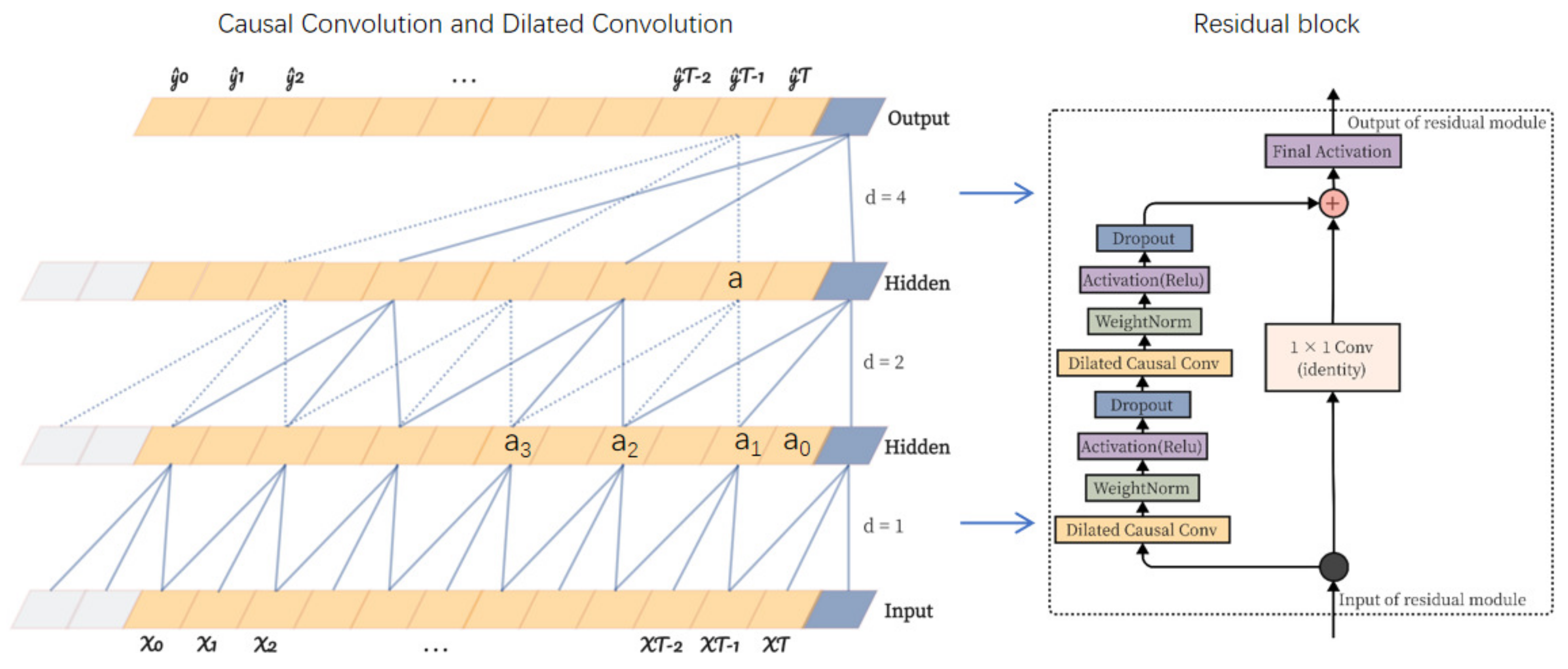
MHA is based on the self-attention mechanism (self attention) [40], which is a method for obtaining contextual information by calculating the correlations between different positions in an input sequence. Since there are many different forms of correlation and many different definitions, it is sometimes not possible to focus on just one form of correlation, but rather on multiple forms of correlation. The MHA allows the model to learn different feature representations at different heads of attention by learning multiple self-attention weight matrices simultaneously. As an example of a three-head attention mechanism, Figure 2 illustrates the structure of an MHA.

2.2. TCN

TCN is composed of causal convolution, dilation convolution, and residual blocks. TCN not only has the advantages of parallelism and temporal causality, but also can flexibly adjust the receptive field, so it is very suitable for processing time series data. Figure 3 shows the block diagram of TCN structure.

Causal convolution can be visualized in Figure 3 (left). The difference with traditional CNN is that causal convolution cannot see future data, and only with the previous cause can we have the subsequent effect, a strictly time-constrained model. A dilated convolution increases the receptive field by injecting holes in the standard convolution to capture longer temporal dependencies. In order to reduce problems such as gradient vanishing brought by too deep a network, TCN introduces a residual block design. The residual block of the TCN is shown in Figure 3 (right).

According to the above description and related papers, a TCN network is very suitable for the PV power time series data forecasting task.

2.3. DC_TCN Model

Since the convolutional kernel size of TCN is fixed, in order to reduce the difficulty of extracting multidimensional spatio-temporal features from the input sequences and to enhance the feature information, this study deeply integrates the input feature data with the model operation mechanism, and innovatively proposes a TCN-based day-ahead photovoltaic power forecasting model with a two-channel structure, DC_TCN. The structure of the proposed model is shown in Figure 4.

The dual-channel architecture is designed with the upper limit of the learning ability of the deep learning model itself in mind. A suitable model’s architecture, and rich input feature information, both help to increase the upper limit of the deep learning model’s learning ability, enabling the model to better adapt to complex patterns and relationships. This study provided diverse input feature information to the model through two channels. At the input feature level, the univariate input channel was used to provide the deep learning model with purely temporal feature information between the sequence elements of the target variables, and the multivariate input channel was used to provide the deep learning model with spatio-temporal feature information between multiple feature variables; and at the level of the channel model selection, the MHA_TCN model was used to simultaneously learn spatio-temporal constraints between other feature variables and the target variables, and the TCN model was used to learn the temporal dependencies between the sequence elements of the target variables alone. More specifically, the model learning process was as follows:

Input Channel 1 of the proposed model was a combination of the multihead attention (MHA) mechanism and the TCN. The target sequence (PV power) and other meteorological sequences together served as its input. Therefore, the input received by the TCN in this channel was a multidimensional vector, and the vector elements were related in both temporal and spatial dimensions, but the actual training was not effective due to the inability to fully utilize the relationships between these inputs, e.g., partial autocorrelation between the internal elements of the PV power generation sequence, and the correlation between this sequence and other meteorological sequences. Therefore, in this paper, MHA was introduced before the TCN, to focus on the spatial correlation between sequences while focusing on the correlation between the elements of each sequence. MHA mapped the multi-feature data to different dimensions, and established a non-linear mapping relationship between PV power and other meteorological variables, paying attention to important spatio-temporal features. These attended features were then used as inputs to the TCN. Although the kernel size of the TCN is fixed, due to its causal and inflated convolutional structure, it can still learn the long-term dependencies of these features through an increasing receptive field according to the temporal constraints of the time series from back to front. Finally, a fully connected neural network (FC) was used to further assign weights to the features extracted by the TCN.

Input Channel 2 of the proposed model was a single TCN which featured only the target sequence (PV power) as input. The causal and dilated convolution of the TCN was utilized to target the extraction of long-term dependencies between the elements of the PV power sequence. Similarly, an FC was used to further assign weights to the features extracted by the TCN.

Finally, the features extracted from the two channels were merged, and the forecasting results were obtained by assigning weights to them through a fully connected neural network, and matching the length of the output forecast sequence.

The dual-channel and combined MHA structural design achieved the deep fusion of PV power generation data with the TCN, which enabled the model to extract more diverse and finer important spatio-temporal features, and reduced the difficulty of the TCN in extracting multi-scale spatio-temporal features from the input sequences.

All the parameters involved in the proposed model are described in detail in Section 4.3 and will not be repeated here.

3. Performance Evaluation Index

In order to evaluate the forecasting performance of the proposed model, the mean absolute error (MAE), the root mean square error (RMSE), and the coefficient of determination (R²) are used in the experiments. Each error is expressed as follows:

$$MAE=\frac{1}{n}{\displaystyle \sum _{i=1}^n\left|y_i-{\widehat{y}}_i\right|}$$

(1)

$$RMSE=\sqrt{\frac{1}{n}{\displaystyle \sum _{i=1}^n{(y_i-{\widehat{y}}_i)}^2}}$$

(2)

$$R^2=1-\frac{{\displaystyle {\sum }_i(}{y}_i-{\widehat{y}}_i{)}^2}{{\displaystyle {\sum }_i{(y_i-{\overline{y}}_{period})}^2}}$$

(3)

4. Case Study

4.1. Experimental Input Data

In this experiment, the data of the DKASC, Alice Springs PV System Site 2 in central Australia, were selected for study. PV system-specific information is shown in Figure 5. The data download address is [41]. Data from January 2014 to January 2016 were selected for this experiment. The data resolution was 15 min for a total of 70,080 data samples. The data consisted of historical power data and other historical meteorological data (collected from the site’s meteorological observatories), and included a total of 12 features. Most previous studies have used the Pearson correlation coefficient method and the Spearman correlation coefficient method as the basis for input feature selection. The Pearson correlation coefficient method requires that the variables obey a normal distribution and can only detect linear relationships; for nonlinear relationships, it may not accurately describe the relationship between two variables. The Spearman correlation coefficient is a nonparametric method that does not require assumptions about the distribution of the data, but it can only capture monotonic relationships between variables and cannot detect nonmonotonic relationships. It is unable to describe complex nonlinear relationships. In view of the above reasons, and considering that deep learning networks have excellent nonlinear feature extraction capabilities, this study did not use correlation analysis alone for feature screening, but rather considered all the features, and ultimately selected the optimal combination of features through experimental trial and error. Finally, active power (kW); global horizontal radiation (w/m² × sr); weather temperature (°C); wind speed (m/s); weather relative humidity (%; and diffuse horizontal radiation (w/m² × sr) were selected as input features. The distribution of each selected feature over time is shown in Figure 6. A total of 90% of the original data was used as a training set, where 80% was used as the training dataset and 20% was used as the validation dataset. A total of 10% of the original data was used as the test set.

4.2. Data Processing

In data preprocessing, firstly, the missing values and outliers in the dataset were replaced by using the prior filling method. Secondly, since different features have different magnitudes, and feature data vary greatly, MinMaxScaler normalization was performed on the training set and test set, respectively, to eliminate the magnitudes in order to speed up the convergence of the model and improve the training efficiency. Finally, the sliding window was utilized to change the input dataset into the input shape (sample, spatio-temporal, and feature) of the deep learning neural network, and then the data form that was convenient for day-ahead forecasting was obtained through sampling and screening. This study performed a day-ahead PV power forecasting task, i.e., a multistep (96 time steps) power forecasting task that forecasts the next 24 h with a time resolution of 15 min. In order to investigate the effect of the input sliding window width on the model performance, seven widths of sliding windows (input time steps) were set, which were 96 timesteps (1 day); 192 timesteps (2 days); 288 timesteps (3 days); 384 timesteps (4 days); 480 timesteps (5 days); 576 timesteps (6 days); and 672 timesteps (7 days), respectively. As an example of the three-day sliding window segmentation method,

Table 1. Training set data at timesteps = 288 (1 day predicted every 3 days).

Samples	Time
Group 1 Sample Data	Start and end time of multi-feature data:	1/1/2014 0:00–3/1/2014 23:45 (288)
	Start and end time of target feature data:	4/1/2014 0:00–4/1/2014 23:45 (96)
Group 2 Sample Data	Start and end time of multi-feature data:	2/1/2014 0:00–4/1/2014 23:45 (288)
	Start and end time of target feature data:	5/1/2014 0:00–5/1/2014 23:45 (96)
…	Start and end time of multi-feature data:	…
	Start and end time of target feature data:	…
Group 653 Sample Data	Start and end time of multi-feature data:	15/10/2015 0:00–17/10/2015 23:45 (288)
	Start and end time of target feature data:	18/10/2015 0:00–18/10/2015 23:45 (96)

demonstrates the specific window sequence segmentation method.

4.3. Experiments and Analysis

In this paper, two sets of experiments were conducted. (1) To verify the performance of the proposed model’s dual-channel structure, ablation experiments were implemented, and the experimental results showed that the dual-channel structure was able to obtain richer, more diverse features, and more accurate forecasting results were achieved. (2) To verify the comprehensive performance of the proposed model, model comparison experiments were conducted, and the forecasting results of the proposed model were compared with those of the current dominant and superior performance of the stacked CNN, and the hybrid CNN_LSTM. CNN and hybrid CNN_LSTM. The experimental results showed that the proposed model obtained significant accuracy improvement. The data flow and parameter settings of the proposed model and the baseline model are shown in Figure 7. All parameters were optimally set by trial and error.

First, ablation experiments were conducted. The MHA_TCN model for channel 1 took both target sequences and other meteorological sequences as input features, and the TCN model for channel 2 took only the target sequences as input features.

Table 2. Ablation Experiment Results.

Models	Evaluation Indicators	Timesteps
		1 Day	2 Days	3 Days	4 Days	5 Days	6 Days	7 Days
TCN	MAE	0.985	1.004	1.005	0.986	1.019	1.025	1.034
	RMSE	1.870	1.871	1.861	1.881	1.923	1.917	1.950
	R2	0.854	0.848	0.851	0.852	0.843	0.845	0.838
MHA_TCN	MAE	0.956	1.017	1.050	1.001	1.030	0.973	0.981
	RMSE	1.919	1.914	1.987	1.969	1.900	2.206	2.073
	R2	0.861	0.846	0.844	0.849	0.839	0.847	0.843
DC_TCN	MAE	0.906	0.987	0.996	0.977	0.999	1.026	1.029
	RMSE	1.776	1.864	1.907	1.881	1.961	1.915	1.882
	R2	0.868	0.856	0.852	0.857	0.842	0.847	0.848

Different color fonts represent different input window widths; bold fonts of different colors represent that the model obtained the best forecasting performance for the input window width corresponding to that color; grey background bold fonts represent the best forecasting results in all models and at all time steps.

shows the forecast performance metrics of the proposed model and the 2-branch channel models when forecasting individually under 7 different input window widths (time steps). The best performance metrics of each model for each input window width are marked with corresponding colors. Figure 8 and Figure 9 show the MAE and RMSE of the 3 models for 7 input time steps, respectively. From the above results, it can be seen that the proposed model obtained the best forecasting results for 1 day’s input window width (96 samples), both when compared horizontally (7 window widths), and vertically (3 models). The MAE was 0.906, which was an improvement of 5.2% with respect to the best MAE for the 2 branching channel models, which was 0.956; the RMSE was 1.776, which was 4.6% higher than the best RMSE of the 2-branch model, with 1.861; and the R² was 0.868, which was 0.8% higher than the best R² of the 2-branch model, with 0.861.

Then, experiments comparing the performance with the baseline model were conducted.

Table 3. Comparative experimental results of CNN, CNN-LSTM, and DC-TCN at different timesteps.

Models	Evaluation Indexes	Timesteps
		1 Day	2 Days	3 Days	4 Days	5 Days	6 Days	7 Days
CNN	MAE	0.957	0.981	0.957	1.010	0.955	1.034	1.036
	RMSE	1.824	1.849	1.836	1.917	1.888	1.932	1.932
	R2	0.859	0.852	0.858	0.848	0.843	0.838	0.836
CNN_LSTM	MAE	0.947	0.970	0.972	0.941	0.950	0.944	0.991
	RMSE	1.829	1.844	1.847	2.016	2.022	2.004	1.869
	R2	0.859	0.857	0.854	0.857	0.854	0.853	0.849
DC_TCN	MAE	0.906	0.987	0.996	0.977	0.999	1.026	1.029
	RMSE	1.776	1.864	1.907	1.881	1.961	1.915	1.882
	R2	0.868	0.856	0.852	0.857	0.842	0.847	0.848

shows the forecasting results of all the models for 7 input window widths. Figure 10 and Figure 11 show the histograms of MAE and RMSE for each model over the 7 input window widths, respectively, from which it can be seen that all models achieved the best forecasting results at an input window width of 1 day (Gray background columns in Table 3). Compared to the other 2 models, the proposed model achieved the best forecasting performance. It can also be seen that for the MAE metric, the performance of the proposed model and CNN showed a decreasing trend with the increase of the input window width, with the proposed model showing the most significant decrease, indicating that the proposed model was relatively sensitive to the window length. The performance of the CNN_LSTM did not show a significant decrease, showing a weaker sensitivity. For the RMSE metrics, similarly, the performance of all 3 models showed a decreasing trend with the increase of input window width, while the CNN_LSTM performance had more ups and downs and showed the worst performance. In order to express the superior performance of the proposed model more finely, Figure 12 demonstrates the percentage accuracy improvement of the proposed model relative to the baseline model when the window length is 1 day: the MAE improved by 5.3% and the RMSE improved by 2.6% compared to the CNN; and the MAE improved by 4.3% and the RMSE improved by 2.9% compared to the CNN_LSTM. The proposed model showed superior forecasting performance. Figure 13 shows the R² of each model, from which it can be seen that the proposed model exhibited the best fit to the data over a 1-day input window length.

In order to demonstrate the forecasting performance of the proposed model more intuitively, Figure 14, Figure 15, Figure 16, Figure 17, Figure 18 and Figure 19 show the curves and scatter plots of the forecast results versus the actual power, for 5 consecutive days under the three weather patterns, respectively. Figure 14 and Figure 15 show the curves and scatter plots under sunny weather patterns. As can be seen from Figure 14, the proposed model exhibited the best fitting performance compared to the baseline model for the majority of the day (power rise and fall phases), while the performance is slightly worse than the baseline model for a small period of time after the power reached its maximum value. The enlarged area of the figure shows that the forecasting curve of the proposed model is closer to the actual power during the power rise phase compared to the other two baseline models, which have more delays; the proposed model is slightly ahead of the baseline model during the power fall phase, while the baseline model’s forecasting was still slightly delayed. Figure 15 shows the corresponding scatter plot of the forecasting results, and it can also be seen from the scatter distribution that the proposed model showed the optimal forecasting performance throughout the forecasting time period, and only performed poorly near the power maximum.

Figure 16 and Figure 17 show the curves and scatter plots for cloudy weather patterns. From Figure 16, it can be seen that none of the 3 models could forecast the fast ramps well, but the proposed model was the best predictor among them, fitting the trend of the actual power better, which was most significant at higher power. Figure 17 shows the corresponding scatter plot of the forecasting results, and it can also be seen from the scatter distribution that during large power fluctuations, the forecasting results of the three models were more dispersed from the actual power value, while in the higher power, the distribution of the forecasting values of the proposed model was closer to the actual power.

Figure 18 and Figure 19 show the curves and scatter plots for rainy weather patterns. It can be seen that the forecast performance of the 3 models was closer to that of the cloudy weather patterns, and in general, the proposed model still had the best overall performance.

In conclusion, the proposed model showed the best forecasting performance regardless of weather patterns. This indicates that the proposed method can extract more useful information from the raw PV power generation data, which makes the model better able to fulfill the task of day-ahead PV power forecasting.

5. Conclusions

In this paper, a novel temporal convolutional neural network (TCN)-based photovoltaic power forecasting method, DC_TCN, is proposed to be applied to a day-ahead photovoltaic power forecasting task. The proposed model innovatively designs two input channels to provide the model with features containing different information to enrich the feature representation. The univariate input channel utilizes the TCN’s inflated convolution and causal convolution structures to target long-term dependencies between the elements of the historical PV power series. The multivariate input channel utilizes the superior multi-feature attention of the multihead attention mechanism (MHA) to learn the correlation between PV power generation data and other meteorological data, which reduces the difficulty for the TCN in extracting multidimensional spatio-temporal features from the input sequences, and improves the feature information. When combined with TCN to learn the long-term spatio-temporal dependence between multivariate sequence elements, ultimately, the features learned from the dual-channel structure are fused and weighted to obtain the forecasting results. The experimental results showed that the proposed model exhibits good forecasting performance on the task of the day-ahead PV power forecasting. The specific findings of this paper are as follows:

(1)

In order to verify the effect of input window width on model performance, all the experiments in this paper were conducted under seven input window widths, and all the experimental results showed that all the models obtain the best performance under a window width of 1 day (96 time steps). The performance of all models showed a decreasing trend with increasing input window width, with the proposed model being the most sensitive to the width of the input window.

(2)

Ablation experiments were carried out in order to verify the feature extraction capability of the proposed model’s dual-channel structure. The experimental results showed that the proposed model obtained better forecasting results compared to the two-branch models, single TCN, and multihead attention combined with the TCN, which also indicates that the design of the dual-channel results can provide more useful feature information for the model and increase the interpretability of the model.

(3)

In order to verify the forecasting performance of the proposed model, comparison experiments were carried out. The experimental results showed that the proposed model achieved better forecasting performance than CNN and CNN_LSTM, which had better performance in PV power forecasting, with a maximum improvement of 5.3% in MAE, and 2.9% in RMSE.

(4)

In addition, it was found that none of the models can forecast fast ramps well on the 15 min resolution data used in the study. While it can be applied to specific application scenarios that do not require high day-ahead ramp forecasting, such as day-ahead generation planning; unit deployment; and day-ahead power market trading, the forecasting value is still insufficient for those day-ahead application scenarios that are sensitive to power ramp changes. In the follow-up study, we will continue to investigate the forecasting performance of the proposed model in terms of both reducing the data resolution, and improving the upper limit of the model’s learning capability, with a view to being able to apply the model to a wider range of application scenarios and improve its applicability.

In conclusion, this paper integrates a model computing mechanism with PV power generation data; innovatively designs the model architecture; provides richer feature information for the model; fully exploits the advantages of each module; and improves the learning ability of the model. The proposed model obtains good performance on the day-ahead PV power forecasting task. In future work, model architectures that can be applied to more time scales will be investigated and applied to PV power forecasting tasks in different application scenarios.

References

1. Net Zero by 2050–Analysis-IEA. Available online: https://www.iea.org/reports/net-zero-by-2050 (accessed on 16 December 2023).
2. Ren, X.; Zhang, F.; Zhu, H.; Liu, Y. Quad-kernel deep convolutional neural network for intra-hour photovoltaic power forecasting. Appl. Energy 2022, 323, 119682. [Google Scholar] [CrossRef]
3. Antonanzas, J.; Osorio, N.; Escobar, R.; Urraca, R.; Martinez-de-Pison, F.J.; Antonanzas-Torres, F. Review of photovoltaic power forecasting. Sol. Energy 2016, 136, 78–111. [Google Scholar] [CrossRef]
4. Ahmed, R.; Sreeram, V.; Mishra, Y.; Arif, M.D. A review and evaluation of the state-of-the-art in PV solar power forecasting: Techniques and optimization. Renew. Sustain. Energy Rev. 2020, 124, 109792. [Google Scholar] [CrossRef]
5. Dolara, A.; Leva, S.; Manzolini, G. Comparison of different physical models for PV power output forecasting. Sol. Energy 2015, 119, 83–99. [Google Scholar] [CrossRef]
6. Celikel, R.; Yilmaz, M.; Gundogdu, A. A voltage scanning-based MPPT method for PV power systems under complex partial shading conditions. Renew. Energy 2022, 184, 361–373. [Google Scholar] [CrossRef]
7. Raza, M.Q.; Nadarajah, M.; Ekanayake, C. On recent advances in PV output power forecast. Sol. Energy 2016, 136, 125–144. [Google Scholar] [CrossRef]
8. Yilmaz, M.; Celikel, R.; Gundogdu, A. Enhanced Photovoltaic Systems Performance: Anti-Windup PI Controller in ANN-Based ARV MPPT Method. IEEE Access 2023, 11, 90498–90509. [Google Scholar] [CrossRef]
9. Srivastava, S.; Lessmann, S. A Comparative Study of Lstm Neural Networks in Forecasting Day-Ahead Global Horizontal Irradiance with Satellite Data. Sol. Energy 2018, 162, 232–247. [Google Scholar] [CrossRef]
10. Wang, H.; Liu, Y.; Zhou, B.; Li, C.; Cao, G.; Voropai, N.; Barakhtenko, E. Taxonomy research of artificial intelligence for deterministic solar power forecasting. Energy Convers. Manag. 2020, 214, 112909. [Google Scholar] [CrossRef]
11. Wang, H.; Yi, H.; Peng, J.; Wang, G.; Liu, Y.; Jiang, H.; Liu, W. Deterministic and probabilistic forecasting of photovoltaic power based on deep convolutional neural network. Energy Convers. Manag. 2017, 153, 409–422. [Google Scholar] [CrossRef]
12. Li, G.; Yang, Y.; Qu, X. Deep learning approaches on pedestrian detection in hazy weather. IEEE Trans. Ind. Electron. 2019, 67, 8889–8899. [Google Scholar] [CrossRef]
13. Guo, Z.; Zhou, K.; Zhang, X.; Yang, S. A deep learning model for short-term power load and probability density forecasting. Energy 2018, 160, 1186–1200. [Google Scholar] [CrossRef]
14. Abdel-Nasser, M.; Mahmoud, K. Accurate photovoltaic power forecasting models using deep LSTM-RNN. Neural Comput. Appl. 2017, 31, 2727–2740. [Google Scholar] [CrossRef]
15. Yao, G.; Lei, T.; Zhong, J. A Review of Convolutional-Neural-Network-Based Action Recognition. Pattern Recogn. Lett. 2019, 118, 14–22. [Google Scholar] [CrossRef]
16. Zhang, J.; Ling, C.; Li, S. EMG Signals based Human Action Recognition via Deep Belief Networks. IFAC Pap. Online 2019, 52, 271–276. [Google Scholar] [CrossRef]
17. Chen, S.; Yu, J.; Wang, S. One-dimensional convolutional auto-encoder-based feature learning for fault diagnosis of multivariate processes. J. Process Control 2020, 87, 54–67. [Google Scholar] [CrossRef]
18. Yang, X.; Cao, M.; Li, C.; Zhao, H.; Yang, D. Learning Implicit Neural Representation for Satellite Object Mesh Reconstruction. Remote Sens. 2023, 15, 4163. [Google Scholar] [CrossRef]
19. Liu, L.M.; Ren, X.Y.; Zhang, F.; Gao, L.; Hao, B. Dual-dimension Time-GGAN data augmentation method for improving the performance of deep learning models for PV power forecasting. Energy Rep. 2023, 9, 6419–6433. [Google Scholar] [CrossRef]
20. Zhang, X.; Yang, Y.; Wang, H.; Zhao, F.; Yan, F.; Wang, M. A Convolutional Neural Network for Regional Photovoltaic Generation Point Forecast. E3S Web Conf. 2020, 185, 01079. [Google Scholar] [CrossRef]
21. Suresh, V.; Janik, P.; Rezmer, J.; Leonowicz, Z. Forecasting solar PV output using convolutional neural networks with a sliding window algorithm. Energies 2020, 13, 723. [Google Scholar] [CrossRef]
22. Bai, S.; Kolter, J.Z.; Koltun, V. An empirical evaluation of generic convolutional and recurrent networks for sequence modeling. arXiv 2018, arXiv:1803.01271. [Google Scholar]
23. Hewage, P.; Behera, A.; Trovati, M.; Pereira, E.; Ghahremani, M.; Palmieri, F.; Liu, Y. Temporal convolutional neural (TCN) network for an effective weather forecasting using time-series data from the local weather station. Soft Comput. 2020, 24, 16453–16482. [Google Scholar] [CrossRef]
24. Lara-Benítez, P.; Carranza-García, M.; Luna-Romera, J.M.; Riquelme, J. Temporal convolutional networks applied to energy-related time series forecasting. Appl. Sci. 2020, 10, 2322. [Google Scholar] [CrossRef]
25. Luo, H.; Dou, X.; Sun, R.; Wu, S. A Multi-Step forecasting Method for Wind Power Based on Improved TCN to Correct Cumulative Error. Front. Energy Res. 2021, 9, 723319. [Google Scholar] [CrossRef]
26. Lin, Y.; Koprinska, I.; Rana, M. Temporal Convolutional Neural Networks for Solar Power Forecasting. In Proceedings of the 2020 International Joint Conference on Neural Networks (IJCNN), Glasgow, UK, 19–24 July 2020; pp. 1–8. [Google Scholar]
27. Limouni, T.; Yaagoubi, R.; Khalid, B.; Khalid, G.; El Houssain, B. Accurate one step and multistep forecasting of very short-term PV power using LSTM-TCN model. Renew. Energy 2023, 205, 1010–1024. [Google Scholar] [CrossRef]
28. Sobri, S.; Koohi-Kamali, S.; Abd Rahim, N. Solar photovoltaic generation forecasting methods: A review. Energy Convers. Manag. 2018, 156, 459–497. [Google Scholar] [CrossRef]
29. Wang, K.; Qi, X.; Liu, H. A comparison of day-ahead photovoltaic power forecasting models based on deep learning neural network. Appl. Energy 2019, 251, 113315. [Google Scholar] [CrossRef]
30. Qu, J.; Zheng, Q.; Pei, Y. Day-ahead hourly photovoltaic power forecasting using attention-based CNN-LSTM neural network embedded with multiple relevant and target variables forecasting pattern. Energy 2021, 232, 120996. [Google Scholar] [CrossRef]
31. Li, P.; Zhou, K.; Lu, X.; Yang, S. A hybrid deep learning model for short-term PV power forecasting. Appl. Energy 2020, 259, 114216. [Google Scholar] [CrossRef]
32. Li, Z.; Xu, R.; Luo, X.; Cao, X.; Du, S.; Sun, H. Short-term photovoltaic power forecasting based on modal reconstruction and hybrid deep learning model. Energy Rep. 2022, 8, 9919–9932. [Google Scholar] [CrossRef]
33. Tovar, M.; Robles, M.; Rashid, F. PV Power forecasting, Using CNN-LSTM Hybrid Neural Network Model. Case of Study: Temixco-Morelos, México. Energies 2020, 13, 6512. [Google Scholar] [CrossRef]
34. Zang, H.; Cheng, L.; Ding, T.; Cheung, K.W.; Liang, Z.; Wei, Z.; Sun, G. Hybrid method for short-term photovoltaic power forecasting based on deep convolutional neural network. IET Gener. Transm. Distrib. 2018, 12, 4557–4567. [Google Scholar] [CrossRef]
35. de Jesús, D.A.R.; Mandal, P.; Chakraborty, S.; Senjyu, T. Solar PV Power forecasting Using a New Approach Based on Hybrid Deep Neural Network. In Proceedings of the 2019 IEEE Power & Energy Society General Meeting (PESGM), Atlanta, GA, USA, 4–8 August 2019; pp. 1–5. [Google Scholar]
36. de Jesús, D.A.R.; Mandal, P.; Velez-Reyes, M.; Chakraborty, S.; Senjyu, T. Data Fusion Based Hybrid Deep Neural Network Method for Solar PV Power Forecasting. In Proceedings of the 2019 North American Power Symposium (NAPS), Wichita, KS, USA, 13–15 October 2019; pp. 1–6. [Google Scholar]
37. Agga, A.; Abbou, A.; Labbadi, M.; El Houm, Y.; Ali, I.H. CNN-LSTM: An efficient hybrid deep learning architecture for predicting short-term photovoltaic power production. Electr. Power Syst. Res. 2022, 208, 107908. [Google Scholar] [CrossRef]
38. Tang, Y.; Yang, K.; Zhang, S.; Zhang, Z. Photovoltaic power forecasting: A hybrid deep learning model incorporating transfer learning strategy. Renew. Sustain. Energy Rev. 2022, 162, 112473. [Google Scholar] [CrossRef]
39. Li, F.; Zheng, H.; Li, X. A novel hybrid model for multi-step ahead photovoltaic power forecasting based on conditional time series generative adversarial networks. Renew. Energy 2022, 199, 560–586. [Google Scholar] [CrossRef]
40. Hu, Y.; Xiao, F. Network self attention for forecasting time series. Appl. Soft Comput. 2022, 124, 109092. [Google Scholar] [CrossRef]
41. DKA Solar Center’s Online Hub for Sharing Solar-Related Knowledge and Data from the Northern Territory, Australia. Available online: http://dkasolarcentre.com.au/download (accessed on 16 October 2022).
Figure 1. Block diagram of research framework of this paper.
Energies 17 00698 g001
Figure 2. Structure of the multihead attention mechanism.
Energies 17 00698 g002
Figure 3. Block diagram of TCN structure.
Energies 17 00698 g003
Figure 4. Structure of proposed model.
Energies 17 00698 g004
Figure 5. Alice Springs PV System Site 2 specific information.
Energies 17 00698 g005
Figure 6. Distribution of each selected feature over time.
Energies 17 00698 g006
Figure 7. Block diagram of data flow and parameter settings for proposed model and baseline model.
Energies 17 00698 g007
Figure 8. MAE of forecasting results for each model over 7 window widths in ablation experiments.
Energies 17 00698 g008
Figure 9. RMSE of forecasting results for each model over 7 window widths in ablation experiments.
Energies 17 00698 g009
Figure 10. MAE of forecasting results for 3 models over 7 window widths.
Energies 17 00698 g010
Figure 11. RMSE of forecasting results for 3 models over 7 window widths.
Energies 17 00698 g011
Figure 12. MAE and RMSE boost percentages for DC_TCN.
Energies 17 00698 g012
Figure 13. R2 line chart of three models.
Energies 17 00698 g013
Figure 14. Forecasting results for 3 models on sunny days.
Energies 17 00698 g014
Figure 15. Scatterplot of sunny day forecast results for 3 models.
Energies 17 00698 g015
Figure 16. Forecasting results for 3 models on cloudy days.
Energies 17 00698 g016
Figure 17. Scatterplot of cloudy day forecast results for three models.
Energies 17 00698 g017
Figure 18. Forecasting results for three models on rainy days.
Energies 17 00698 g018
Figure 19. Scatterplot of rainy day forecast results for 3 models.
Energies 17 00698 g019