Article

A Multi-Step Ensemble Approach for Energy Community Day-Ahead Net Load Point and Probabilistic Forecasting

by
Maria da Graça Ruano
1,2,* and
Antonio Ruano
1,3,*
1
Faculty of Science & Technology, University of Algarve, 8005-294 Faro, Portugal
2
CISUC, University of Coimbra, 3030-290 Coimbra, Portugal
3
IDMEC, Instituto Superior Técnico, Universidade de Lisboa, 1049-001 Lisbon, Portugal
*
Authors to whom correspondence should be addressed.
Energies 2024, 17(3), 696; https://doi.org/10.3390/en17030696
Submission received: 7 January 2024 / Revised: 26 January 2024 / Accepted: 28 January 2024 / Published: 31 January 2024
(This article belongs to the Section F5: Artificial Intelligence and Smart Energy)

Abstract

:
The incorporation of renewable energy systems in the world energy system has been steadily increasing during the last few years. In terms of the building sector, the usual consumers are becoming increasingly prosumers, and the trend is that communities of energy, whose households share produced electricity, will increase in number in the future. Another observed tendency is that the aggregator (the entity that manages the community) trades the net community energy in public energy markets. To accomplish economically good transactions, accurate and reliable forecasts of the day-ahead net energy community must be available. These can be obtained using an ensemble of multi-step shallow artificial neural networks, with prediction intervals obtained by the covariance algorithm. Using real data obtained from a small energy community of four houses located in the southern region of Portugal, one can verify that the deterministic and probabilistic performance of the proposed approach is at least similar, typically better than using complex, deep models.

1. Introduction

The increased incorporation of renewable energy systems (RES) in the world’s energy system, replacing traditional thermal power stations, has translated into important advantages in the reduction of atmospheric pollutants. Concerning the building sector, residential end-user normal consumers are changing to be active prosumers (i.e., those who consume and produce energy), proactively managing their energy demands by employing home energy management systems (HEMS) and, in some cases, using energy storage systems. Surplus electricity can be, in most cases, traded with grid companies.
This completely decentralized approach, however, has also disadvantages. From the grid point of view, it can introduce instability, resulting in increased interactions and unpredictable fluctuations; from the prosumers’ point of view, it is not as beneficial as expected since, generally, there is a large difference between buying and selling electricity tariffs. Due to these reasons, the concept of sharing and exchanging electricity between prosumers has emerged as a promising solution for achieving collective benefits. Energy communities made up of interconnected loads and distributed energy resources, can employ energy-sharing strategies that maximize community self-consumption and reduce dependence on the central grid. Different energy-sharing strategies are discussed in [1], where it is assumed that each community member has an intelligent home energy management system (HEMS) managing its own flow of energy under the supervision of an intelligent aggregator that controls the whole energy community and also responsible for the community’s interaction with the central grid. Other approaches have been reported in the literature, such as the use of reinforcement learning for energy management of island groups [2].
In recent years, in many countries, the acquisition and sale of electricity is traded in energy markets [3,4]. Accurate forecasts of the electricity demand and price are therefore a necessity for the participants in the energy markets. In particular, the one-day ahead (1DA) hourly forecast, considered a short-term forecast, has received increasing attention from the research community. Comprehensive reviews on load and price forecasting are available in [5,6] and [7,8] respectively. Works on load demand and price forecasts for several energy markets can be found in [9], for the Spanish market in [10] and for the Portuguese energy market in [11].
This paper assumes the scenario of a community of energy managed by an aggregator. Additionally, it is also considered that the aggregator will buy the electricity needed by the community in an energy market, such as the Iberian Electricity Market—MIBEL. The MIBEL day-ahead market is the system in which electricity is traded for delivery the day after it is traded. This market has prices for every hour of each day. Every day, this platform receives bids until 12 noon. Those bids will feed an algorithm that will compute electricity prices for the following day.
To manage the community efficiently, the aggregator needs to employ good forecasts of the day-ahead net energy or power required, as well as the future selling/buying prices. This paper will deal only with the day-ahead net power and will assume that day-ahead prices are obtained by other techniques. As the net power is the difference between the load demand and the electricity produced, good forecasts of both variables are required. In addition, if the aggregator manages different communities of energy, these forecasts should be extended to the aggregation of all day-ahead net energy foreseen.
Existing load and generation forecasting algorithms can be classified into two classes: point forecasts and probabilistic forecasts [12]. The former provides single estimates for the future values of the corresponding variable, which are not capable of properly quantifying the uncertainty attached to the variable under consideration. The latter algorithms are increasingly attracting the attention of the research community due to their enhanced capacity to capture future uncertainty, describing it in three ways: prediction intervals (PI), quantiles, and probability density functions (PDF) [13]. PI-based methods are trained by optimizing error-based functions and constructing the PIs using the outputs of the trained prediction models [14]. Traditional PI methods are the Bayesian [15], Delta [16], Bootstrap [17] and mean-variance (MVE) [18] techniques. In this paper, we shall be using the covariance method, which was introduced in [19] and discussed later on.
Specifically for load demand point forecasting, the works [20,21,22] can be highlighted. In the former, data from four residential buildings, sampled with an interval of 15 min, is employed. Three forecasting models are compared: (i) the Persistence-based Auto-regressive (AR) model, (ii) the Seasonal Persistence-based Regressive model, and (iii) the Seasonal Persistence-based Neural Network model, as well as mixtures of these three methods.
Kiprijanovska and others [21] propose for forecasting a deep residual neural network, which fuses different sources of information by extracting features from (i) contextual data (weather, calendar) and (ii) historical load of the particular household and all households present in the dataset. Authors compared their approach with other techniques on 925 households of the Pecan Street database [23] with data re-sampled at 1 h time interval. Day-ahead forecasts are computed at 10 h, the previous day. The proposed approach achieves excellent results in terms of RMSE, MAE, and R2.
Pirbazari and co-authors [22] employed hourly data from a public set of 300 Australian houses available from 2010 to 2013. This set consisted of load demand and electricity generation for the six hundred houses, which have, for analysis, been divided into six different 50-house groups. For forecasting, they propose a method that, firstly, considers highly relevant factors and, secondly, benefits from an ensemble learning method where one Gradient Boosted Regression Tree algorithm is joined with several Sequence-to-Sequence Long Short-Time Memory networks. The ensemble technique obtained the best 24-h-ahead results for both load and generation when compared to other isolated and ensemble approaches.
Focusing now on PV generation point forecasting, the work [24] should be mentioned. The authors propose an LSTM-attention-embedding model based on Bayesian optimization to forecast photovoltaic energy production for the following day. The effectiveness of the proposed model is checked on two real PV power plants in a Chinese area. Comparative results allow us to conclude that the performance of the proposed model has been considerably improved compared to Long Short-Time Memory neural networks, Back-Propagation Neural Networks, Support Vector Regression machines, and persistence models.
The works cited above deal with point forecasting. We shall now move to a probabilistic forecasting survey.
Jaun Vilar et al. [9] propose two techniques for obtaining PIs for electricity and price demand using functional data. The first technique uses a non-parametric AR model, and the second one uses a partial linear semi-parametric model, where exogenous covariates are employed. In both procedures for the construction of the PIs, residual-based bootstrap algorithms are used, allowing estimates of the prediction density to be obtained. The 2012 entire year of the total load demand in Spain is employed, using an hourly sampling time. It has been found that using the Winkler score, the second method obtains better results.
Zhang and co-workers [12] propose a probability density prediction technique based on monotone composite quantile regression ANN and Gaussian kernel function (MCQRNNG) for day-ahead load. Employing real load data carrying quantile crossing from Ottawa in Canada, Baden-Württemberg in Germany, and a region in China, the performance of the MCQRNNG model is verified from three aspects: point, interval, and probability prediction. Results show that the proposed model improves the comparison model based on the effective elimination of quantile crossing for energy load forecasting.
Regarding PV generation, refs. [25,26] should be mentioned. The former compares the suitability of a non-parametric distribution and three parametric distributions in characterizing prediction intervals for photovoltaic energy forecasts with high levels of confidence. The calculations were carried out for one year of next-day forecasts of the hourly energy production of 432 photovoltaic systems. The results showed that, in general, the non-parametric distribution hypothesis for the forecast error produced the best forecast intervals.
Mei et al. [26] propose an LSTM-Quantile Regression Averaging (QRA)--based non-parametric probabilistic forecasting model for PV output power. Historical data was collected on photovoltaic output power, global horizontal irradiance, and temperature from a roof-mounted photovoltaic power generation system in eastern China. This data was analyzed to detect outliers and extreme values were eliminated. An ensemble of independent deterministic LSTM forecasting models is trained using historical photovoltaic data and numerical weather prediction (NWP) data. The non-parametric probabilistic forecast is generated by integrating the independent LSTM forecast models with Quantile Regression Averaging (QRA). Compared to the reference methods, LSTM-QRA has a superior forecasting performance due to the better accuracy of the independent deterministic forecasts.
Finally, ref. [27] seems to be the only publication looking at the net load forecasting of residential microgrids. The authors propose a data-driven-based net load uncertainty quantification fusion mechanism for cloud-based energy storage management with renewable energy integration. First, a fusion model is developed using SVR, LSTM, and Convolutional Neural Network—Gated Recurrent Unit (CNN-GRU) algorithms to estimate day-ahead load and PV power forecasting errors. Subsequently, two techniques are employed to obtain the day-ahead net load error. In the first approach, the net load error is predicted directly, while in the second technique, it is derived from the load and photovoltaic energy prediction errors. The uncertainty is analyzed with various probability confidence intervals. However, those are not prediction intervals, and this way, the actual data does not lie within those bounds. Additionally, the forecasts are computed at the end of one day for the next 24 h, i.e., the PH is only 24 h and cannot be used for energy markets.
The present paper solves the issues mentioned in relation to the last reference. It allows the community(s) managed by an aggregator to obtain excellent day-ahead hourly point forecasts of the net load, whose robustness can be accessed by prediction intervals obtained at a user-specified confidence level. This allows the aggregator to make more informed decisions regarding energy trading.
This is achieved using robust ensemble forecasting models, which will be described in Section 2. The data employed and the results obtained are presented in Section 3. They are discussed in Section 4 and compared with results obtained by other works. Section 5 concludes the paper.

2. Material and Methods

The design of robust ensemble forecasting models has been discussed elsewhere (please see [28]) and will only be summarized here.
To design “good” single models from a dataset of design data, three sub-steps must be followed:
  • data selection—given the design data, suitable sets (training, testing, validation, …) must be constructed.
  • features/delays selection—given the above data sets, the “best” inputs and network topology should be determined.
  • parameter estimation—given the data sets constructed and using the inputs/delays and network topology chosen, the “best” network parameters should be determined.
These steps are solved by two existing tools. The first, ApproxHull, implements the first sub-step. The second sub-step is achieved by the genetic part of MOGA (Multi-Objective Genetic Algorithm), while the gradient component of MOGA implements the third sub-step.

2.1. Data Selection

To obtain good data-driven models within the domain where the underlying process is supposed to operate, it is mandatory that the samples that enclose that domain are present in the training set. These samples, denoted as convex hull (CH) points, can be determined by convex hull algorithms.
As real CH algorithms have an NP time and space complexity, they are useless for high dimensions. Therefore, we have proposed in [29] a randomized approximation convex hull algorithm, denoted as ApproxHull, proposed.
Previously, to determine the CH points, ApproxHull eliminated replicas and linear combinations of samples/features. The CH points identified by the algorithm are incorporated in the training (tr), and test (te) and validation (val) are also created.

2.2. MOGA

This framework is detailed in [30], and it will be briefly discussed here.
MOGA designs static or dynamic ANN (Artificial Neural Network) models for classification, approximation, or forecasting purposes.

2.2.1. Parameter Separability

MOGA works with models Radial Basis Function (RBF) networks, Multilayer Perceptrons, B-Spline and Asmod models, and Wavelet networks, as well as Mamdani, Takagi, and Takagi-Sugeno fuzzy models (satisfying certain assumptions) [31]. These models have the common characteristic that their parameters are linear-non-linearly separable [32]. The output of these models, at sample k, is obtained as:
y ^ x k , w = u 0 + i = 1 n u i φ i x k , v i = φ x k , v u
In (1), x k is the kth input sample of length d, φ denotes the basis functions vector, the output weights that appear linearly in the output are captured in vector u, and v denotes the parameters that appear non-linearly in the output. Assuming for simplicity in this paper only one hidden layer v is composed of n sets of parameters, each for each neuron v = v 1 v n T .
RBF models will be used here. The non-linear basis functions employed are typically Gaussian functions:
φ i x k , v i = e x k c i 2 2 2 σ i 2
The non-linear parameters for each neuron are, therefore, the center vector, c i , with as the same length as the input (d), and a spread parameter σ i .
There are typically heuristics that can be employed to initialize the non-linear parameters. For RBFs, center values can be initialized with random values. Another approach involves clustering algorithms. Several heuristics can be employed for the spreads, such as:
σ = z m a x 2 n ,
where zmax is the maximum distance between the centers.
For the general case, the parameters for linear–non-linearly separable models can be separated into linear (u) and non-linear (v):
w = u v ,
For a set of m input patterns X, training the model means usually determining w, by minimizing (5):
Ω X , w = y y ^ X , w 2 2 2
where y is the target vector, y ^ is the RBF output vector and . 2 is the Euclidean norm. Substituting (1) in (5), we have:
Ω X , w = y Γ X , v u 2 2 2 ,
where Γ X , v = φ x 1 , v φ x m , v T . As (6) is a linear problem in u, its global optimal solution with respect to u is given as:
u * = Γ + X , v y
The symbol ‘+’ represents a pseudo-inverse operation. Replacing (7) in (6), we obtain a new criterion dependent only on v:
Ψ X , w = y Γ X , v Γ + X , v y 2 2 2  

2.2.2. Training Algorithm

Any gradient algorithm can be employed to minimize (6) or (8). As these are non-linear least-squares problems, methods that exploit the sum-of-squares characteristics of the problem should be employed. The Levenberg-Marquardt (LM) technique [33,34] is recognized to be the state-of-the-art method for this class of problems. The LM search direction at iteration k ( p k ) is given as the solution of:
J k T J k + λ k I p k = g k ,
where g k is the gradient vector:
g k = δ Ω k δ w k or δ Ψ k δ v k
and J k is the Jacobean matrix:
J k = δ y ^ k δ w k or δ y ^ k δ v k
The parameter λ is a regularization parameter, which allows the search direction to alternate between the steepest descent and the Gauss-Newton directions. It was proved that the gradient and Jacobean of criterion (8) can be obtained by (1) computing u * using (7); (2) replacing u * in the linear parameters of the model; and (3) computing the gradient and Jacobian in the standard way.
In MOGA, the training algorithm ends after a user-defined number of iterations or by using an early-stopping technique [35].

2.2.3. The Evolutionary Part

MOGA evolves ANNs (in the case of the present paper, RBFs) structures, whose parameters separate, each structure trained by the LM algorithm minimizing (8). We shall be using multi-step-ahead forecasting, and this way, each model should be iterated PH times to forecast the evolution of a variable within a selected Prediction Horizon (PH). For each step, model inputs evolve with time. Consider a Non-linear Auto-Regressive model with Exogenous inputs (NARX) where, for simplicity, 1 input, x is used:
y ^ k + 1 | k = f y k d o 1 , , y k d o n , x k d i 1 , , x k d i m ,
In (12) y ^ k + 1 | k denotes the forecast for time-step k + 1 given the data measured at instant k, and d k j the jth delay for variable k. Equation (12) represents the one-step-ahead (1SA) forecast within PH. As (12) is iterated, some or all the indices on its right-hand side will be larger than k, which indicates that there are no available measured values. In this case, the respective forecasts must be used. What has been said for NARX models is also valid for NAR models (models with no exogenous inputs).
The genetic part of MOGA evolves a population of ANN models. Each structure consists of the number of neurons in the single hidden layer and the model inputs. MOGA considers that the number of neurons, n, must be within a user-specified range n n m , n M . Additionally, the user can select the number of inputs to use for a specific model. It is assumed that, from a total number q of available features, each model will select the most representative d features within a user-specified interval, d d m , d M , d M q , dm representing the minimum number of features, and dM its maximum number.
The operation of MOGA is a typical genetic process, where the operators were conveniently changed to implement topology and feature selection and make sure that there are no models with an equal structure. The reader can consult publication [30] for a more detailed explanation of MOGA.
MOGA is a multi-objective optimizer; this way, the optimization objectives and/or goals need to be specified. Typical objectives are Root-Mean-Square Errors (RMSE) evaluated on the training set ( ρ t r ) or on the test set ( ρ t e ), as well as the model complexity #(v), or yet the norm of the linear parameters ( u 2 ). For forecasting applications, one additional criterion is usually employed. The user selects a time series sim with p data points from the available design data. For each point, (12) is used to make forecasts up to PH steps ahead. An error matrix is then created:
E s i m , P H = e 1,1 e 1 , P H e p P H , 1 e p P H , P H ,
where e[i,j] is the model prediction error obtained for instant i of sim at step j within PH. Assume that ρ s i m . , i , is the RMS operating over the ith column of matrix E . The prediction performance can then be assessed by (14):
ρ s i m s i m , P H = i = 1 P H ρ s i m E s i m , P H , i
Notice that in the MOGA formulation, every performance criterion can either be minimized or set as a goal to be met by the models.
After formulating the optimization problem, in terms of the performance criteria, range of inputs and neurons, and setting hyperparameters such as the number of elements in the population (npop), number of iterations (niter), as well as genetic algorithm parameters (proportion of random immigrants, selective pressure, crossover rate, and survival rate), MOGA can be executed.
After MOGA has concluded its execution, performance values of npop * niter different models are available. As the problem is multi-objective, there is no single optimal solution; rather a subset of these models corresponding to Pareto solutions or non-dominated models (nd) must be examined. If one or more objectives is/are set as goal(s) to be met, then a subset of nd, denoted as preferential solutions, or pref (non-dominated solutions that met the goals) is checked.
MOGA performance is assessed on nd or in pref sets. If a single solution is desired, it will be chosen by the user based on the objective values of the models belonging to those sets, on the validation set, and possibly on other criteria.
For any problem, MOGA is typically executed at least two times. In the first execution, all objectives are minimized, and model parameters are set to standard values. By analyzing the results obtained in this initial execution, the problem definition steps can be revised by (a) input space redefinition, (b) redefining model ranges, and (c) improving the trade-off surface coverage.

2.3. Model Ensemble

According to the previous discussion, a MOGA output is not one single RBF, but sets of non-dominated or preferential RBFs. The models within these sets are typically excellent models, all with a different structure, which can be employed as a stacking ensemble.
Several different approaches have been applied to ensemble models. To be employed in computationally intensive tasks, a simple technique, computationally speaking, of combining the outputs of the model ensemble should be used. In our case, as a few outliers have been generated, a median of the models in the ensemble is employed:
y ˘ = m e d i a n y ^ i , i   ϵ   o u t s e t ,   n o u t   o d d y m 1 : y m 1 , y m 2   a r e   t h e   m i d d l e   v a l u e s   o f   t h e   s o r t e d   o u t s e t ,   n o u t   e v e n ,
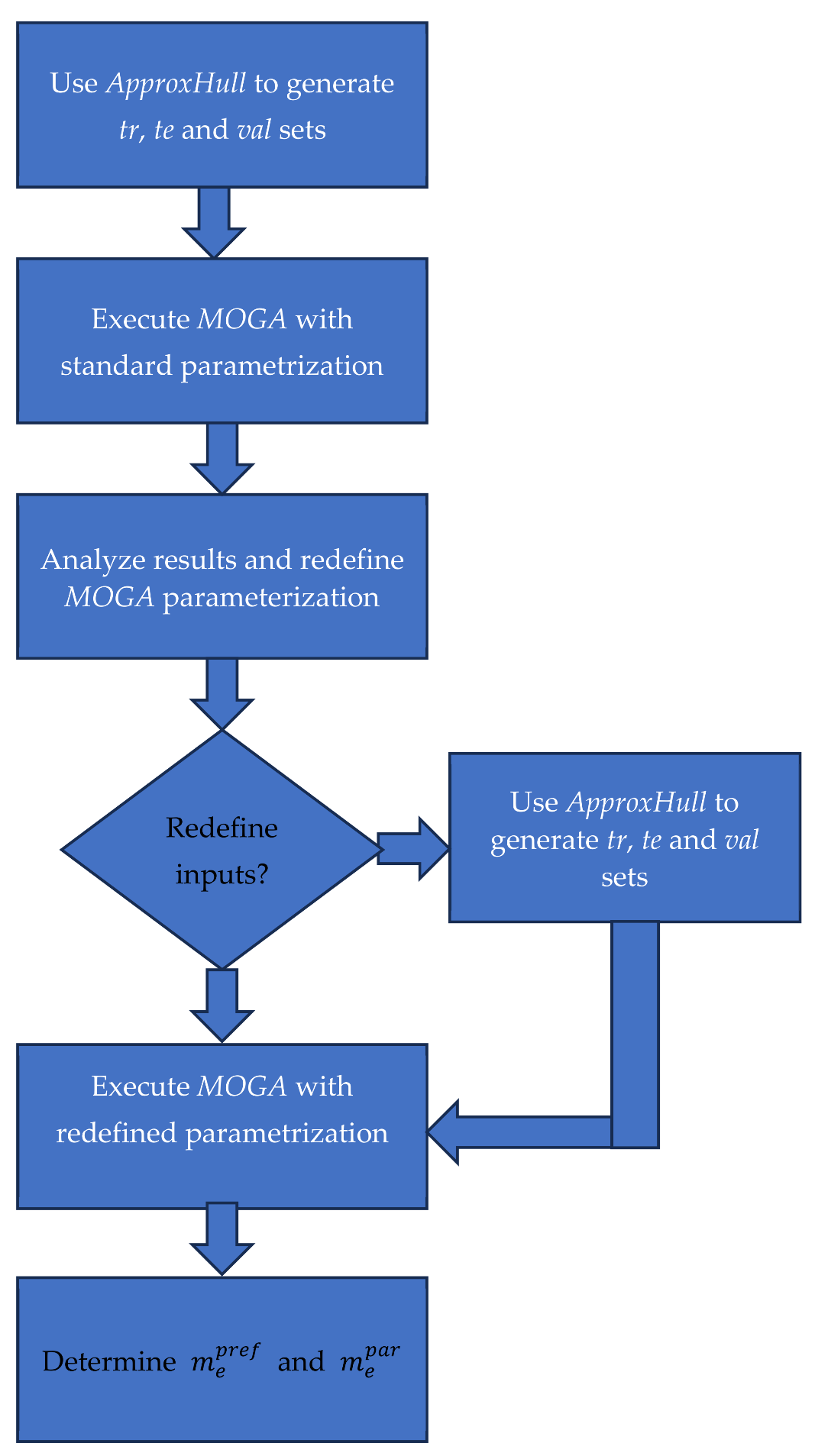
In (15), the set of models is denoted as outset and n o u t being the number of elements at the outset. It was argued in [28] that 25 was a convenient number of elements for the outset and that its elements should be selected using a Pareto concept. The sequence of procedures that should be followed for model design is presented in Figure 1.
In this fluxogram, m e p r e f is obtained as:
m e p r e f = m p r e f : n w m p r e f m ˘ n w p r e f m p r e f : f o r e m p r e f m ˘ f o r e p r e f ,
where m p r e f represents the set of preferential models obtained in the second MOGA execution, m ˘ n w p r e f = m e d i a n n w m p r e f , m ˘ f o r e p r e f = m e d i a n f o r e m p r e f . n w m p r e f denotes the linear weight 2-norm for each model in m p r e f , m ˘ n w p r e f is its median. f o r e m p r e f denotes the forecasts for the prediction time series achieved for all models in m p r e f , computed using (14), being m ˘ f o r e p r e f its median.
From m e p r e f the set of m e p a r models to employ in the ensemble are obtained by determining the 25 models with a good compromise between the forecast fore(.) and the norm of the linear parameters nw(.) of each model:
m e p a r = n d f o r e m e p r e f , n w m e p r e f : # n d = 25
This set is obtained iteratively until 25 models are found by adding preferential models, considering and fore(.) as the two criteria. The set of models to be inspected, m i , i = 1 is initialized to m e p r e f , and m e p a r to an empty set. In each iteration, both criteria are computed for the models in m i . Non-dominated solutions found are added to m e p a r and removed from m i .
Please note that if the model is a NARX model, the forecasts of each exogenous variable should be employed as inputs to the NARX model. This means that for each dynamic exogenous variable, a NAR (or NARX) model should be designed using the operations present in Figure 1. Afterwards, when designing the NARX model, the model ensemble m e p a r for each exogenous variable should be used.

2.4. Robust Models

The recent inclusion of smart grids and renewable integration requirements had the consequence of increasing the uncertainty of future prices, supply, and demand. For this reason, probabilistic electricity price, load, and production forecasting is increasingly required for energy systems planning and operations [8,36].
We assume that all observations are obtained by a data generating function f(x), contaminated with additive output noise:
y k = f z k = y ^ k + ε k
where y ^ k represents the point forecast of y at time k obtained using data available at an earlier point in time and ε k is a data noise term representing uncertainty, which can be decomposed into three terms:
  • training data uncertainty, related to the representativity of the training samples in the model’s whole operational range; in our approach, ApproxHull tries to minimize the first type of uncertainty by including CH points in the training set;
  • model misspecification: the model, with its global optimal parameters and data operational range, is only an approximation of the real function generating the data; in our approach, an ensemble of models is employed, whose structures are the result of an evolutionary process, and
  • parameter uncertainty, related to the fact that the parameters employed in the model might not be the optimal ones even if the structure is the optimal one; this is minimized in our approach by using state-of-the-art gradient methods with different parameter initializations.
The most common method to evolve from point to probabilistic forecasts is to compute prediction intervals (PIs). Please notice that a (1 − α) PI implies that the computed interval contains the true value with a probability of (1 − α). If this is transferred to the calculation of quantiles, this corresponds to τ = α/2 for the lower bound and τ = (1 − α/2) for the upper bound [37]. 90% of PIs will be used in this paper. We will denote y ^ ¯ k and y ^ _ k the upper and lower bounds, respectively.
There are diverse ways to compute the PIs. The interested reader can consult [14], which describes different possibilities. In our case, the covariance method introduced in [19] will be employed. Using the notation Γ X , v , introduced in Section 2.2.1 to indicate the output matrix of the hidden layer, which is dependent on X and on v, the total variance for each forecast y ^ k can be computed [19] as:
σ t o t 2 = σ ε 2 1 + φ T x k , v Γ T Z t r , v Γ Z t r , v 1 φ x k , v
where Z t r is the input training matrix, and the data noise variance, σ ε 2 , can be estimated as:
σ ε 2 = i = 1 N e i 2 N p = i = 1 N y i y ^ z i 2 N p ,
In (20), N represents the total number of samples, and p is the number of model parameters. The bounds, assumed to be symmetric, are:
y ^ k _ = y ^ k Δ y ^ k y k y ^ k + Δ y ^ k = y ^ k ¯
Δ y ^ k = t 1 α 2 , N p σ t o t
where t 1 α / 2 , N p is the α/2 quantile of a Student’s t-distribution with Np degrees of freedom.
The optimal values obtained after training, Γ Z t r , v * and φ x k , v * , can be employed in (19). In fact, due to the MOGA design, these two quantities are already available, provided that x k belongs to the test or validation sets. This way, it is computationally cheap to compute (19).
We shall be denoting as robust models the ones whose outputs lie within PIs computed with a user-specified level of confidence.

2.5. Robust Ensemble Forecasting Models

For every time instant k, we are interested in determining PH forecasts y ^ k + s | k , s 1 P H , together with the corresponding bounds Δ y ^ k + s | k , s 1 P H .
As we are dealing with an ensemble of models and using the notation introduced in (15), we shall denote the forecasts as y ˘ k + s | k to signify that, at each step, we shall be using the median value of the ensemble of values computed using (15).
In the same way, the corresponding bound will be denoted as Δ y ˘ k + s | k and φ x k , v and Γ Z t r , v in (19) will be denoted as φ ˘ x k , v ˘ and Γ ˘ Z ˘ t r , v ˘ . Therefore, (19)–(22) should be replaced by:
σ ˘ t o t 2 ( s ) = σ ˘ ε 2 ( s ) ( 1 + φ ( s ) T ( x k + s , v ( s ) ) ( Γ ˘ T ( Z ˘ t r , v ( s ) ) Γ ˘ ( Z ˘ t r , v ( s ) ) ) 1 φ ( s ) ( x k + s , v ( s ) ) )
σ ˘ ε 2 ( s ) = k = 1 N e ˘ k + s 2 N p ˘ = k = 1 N y k + s y ˘ k + s k z k 2 N p ˘
y ˘ _ k + s | k = y ˘ k + s | k Δ y ˘ k + s | k y k y ˘ k + s | k Δ y ˘ k + s | k = y ˘ ¯ k + s | k
Δ y ˘ k + s | k = t 1 α 2 , N p ˘ σ t o t ( s )

2.6. Performance Criteria

Several criteria will be employed to evaluate the quality of the models.
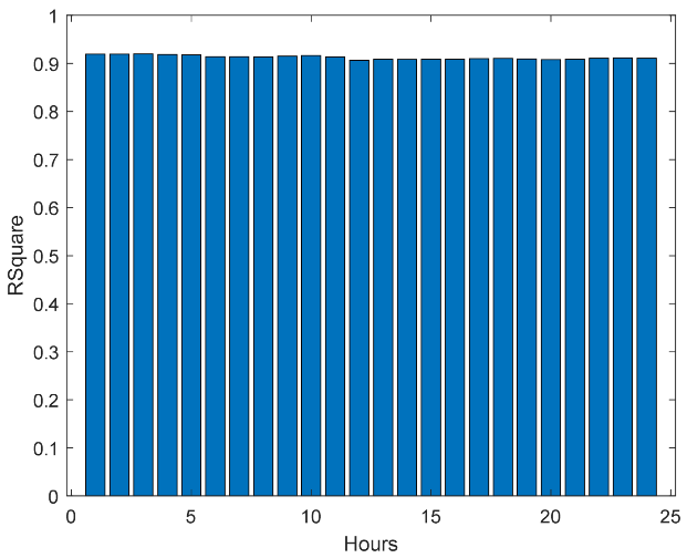
For point forecasting, we shall use Root-Mean-Square of the Errors (RMSE) (27), Mean-Absolute Error (MAE) (28), Mean-Absolute Percentage Error (MAPE) (29), and Coefficient of Determination or R-square (R2) (30). As the performance of the forecasts should be assessed not only for the 1SA but also along PH, all the different indices will be averaged over the Prediction Horizon. For all indices, N is the number of samples considered.
R M S E ¯ = 1 P H s = 1 P H R M S E ( s ) ,   R M S E s = k = 1 N y k + s y ^ k + s k 2 N
M A E ¯ = 1 P H s = 1 P H M A E ( s ) ,   M A E s = k = 1 N y k + s y ^ k + s k N
M A P E ¯ = 1 P H s = 1 P H M A P E ( s ) ,   M A P E s = 1 N k = 1 N y k + s y ^ k + s k y k + s
y ̿ s = 1 N k = 1 N y k + s S S R e s s = k = 1 N y k + s y ^ k + s k 2 S S T o t s = k = 1 N y k + s y ̿ s 2 R 2 s = 1 S S R e s s S S T o t s R 2 ¯ = 1 P H s = 1 P H R 2 s
Some measures have been proposed related to the robustness of the solutions. One of the simplest is the Average Width (AW):
A W ( s ) = 1 N k = 1 N W k s ,
where the width is given as:
W k s = y ˘ ¯ k + s | k y ˘ _ k + s | k
In (32), y ˘ ¯ k + s | k and y ˘ _ k + s | k are the upper and lower bounds, introduced in (25), of the model output for time k + s, given data available until time k, respectively.
A more sophisticated measure of interval width is the Prediction Interval Normalized Averaged Width (PINAW), defined as:
  P I N A W s = 1 R A W ( s ) = 1 N R k = 1 N y ˘ ¯ k + s | k y ˘ _ k + s | k ,
R is the range of the whole prediction set:
R = m a x y m i n y .
On the other hand, if we are interested in the magnitude of the violations, we can use the Interval-based Mean Error (IME), also called the PI Normalized Average Deviation (PINAD):
P I N A D ( s ) = 1 N k = 1 N I M E k s ,
I M E k s = y ˘ _ k + s | k y k + s R , y k + s < y ˘ _ k + s | k 0 , y ˘ _ k + s | k y k + s y ˘ ¯ k + s | k y ˘ ¯ k + s | k y k + s R , y k + s > y ˘ ¯ k + s | k
To assess the coverage, we can use the Prediction Interval Coverage Probability (PICP). PICP verifies if the interval y ˘ _ k + s | k , y ˘ ¯ k + s | k contains the real measure of y k + s :
  P I C P ( s ) = 1 N k = 1 N c k ( s ) ,
where
c k s = 1 ,     i f     y ˘ _ k + s | k y k + s y ˘ ¯ k + s | k 0 ,                                                   o t h e r w i s e
Another metric that is often used to assess both the reliability and the sharpness of the PIs is the Winkler Score [38]. As can be seen, it penalizes the interval width with the magnitude of the violations, weighted proportionally by the confidence level.
W S ( s ) = 1 N k = 1 N W S k s ,
W S k s = A W ( s ) + 2 α   y ˘ _ k + s | k y k + s , y k + s < y ˘ _ k + s | k A W ( s ) ,   y ˘ _ k + s | k y k + s y ˘ ¯ k + s | k A W s + 2 α y k + s y ˘ ¯ k + s | k , y k + s > y ˘ ¯ k + s | k
The previous criteria must be averaged over PH:
A W ¯ = 1 P H s = 1 P H A W s
P I N A W ¯ = 1 P H s = 1 P H P I N A W s
P I N A D ¯ = 1 P H s = 1 P H P I N A D s
P I C P ¯ = 1 P H s = 1 P H P I C P s
W S ¯ = 1 P H s = 1 P H W S s

3. Results

3.1. The Data

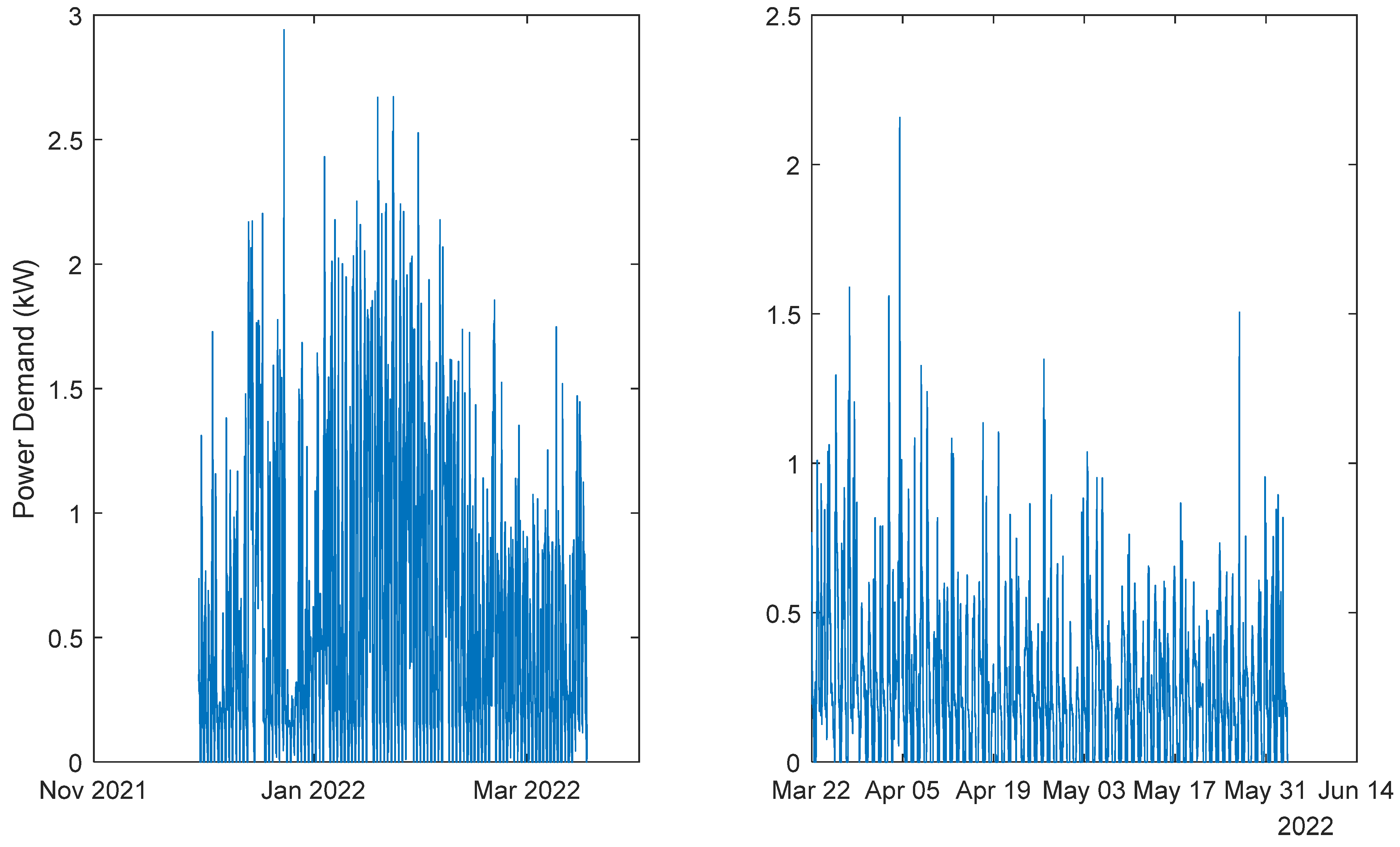
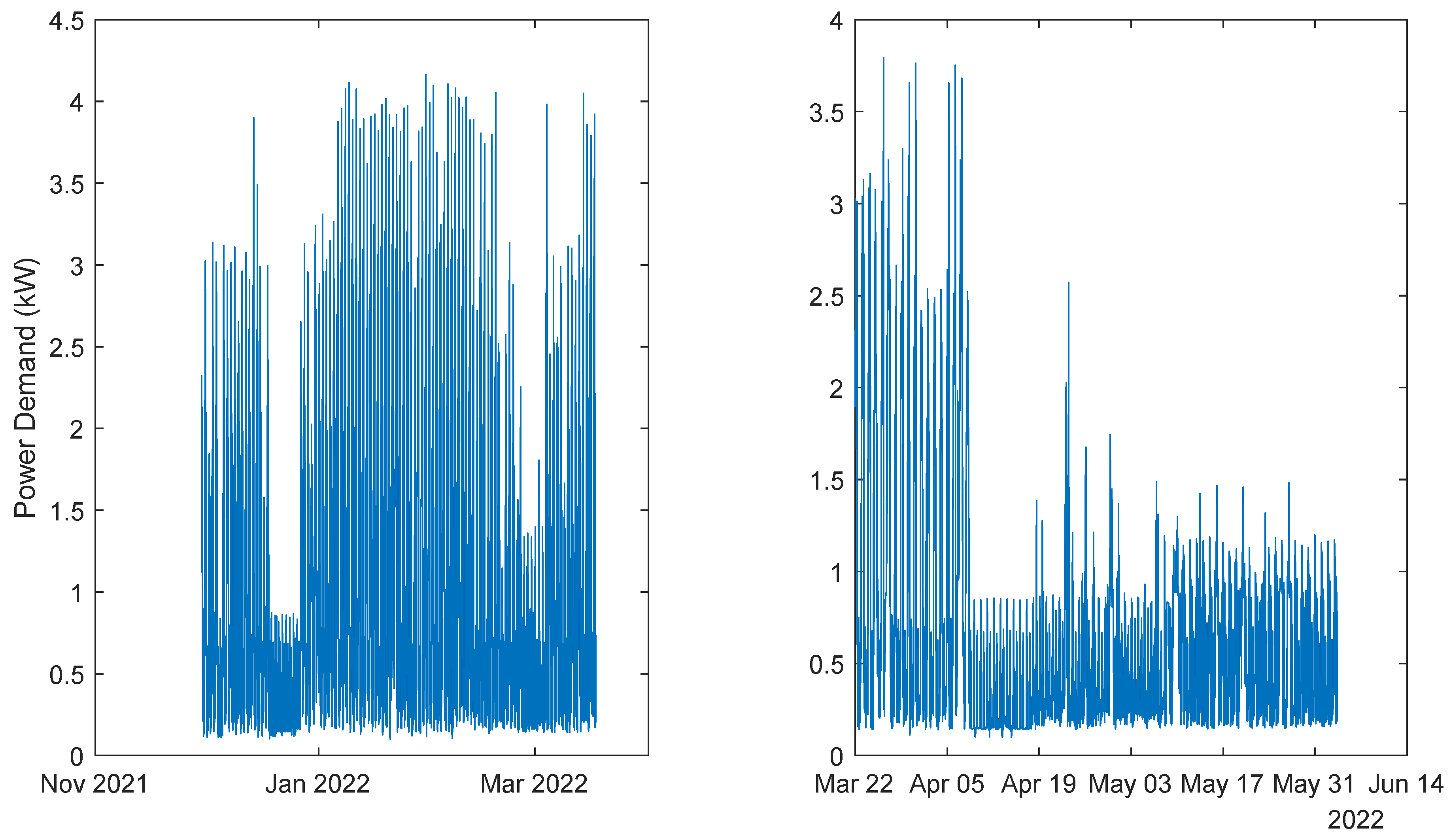
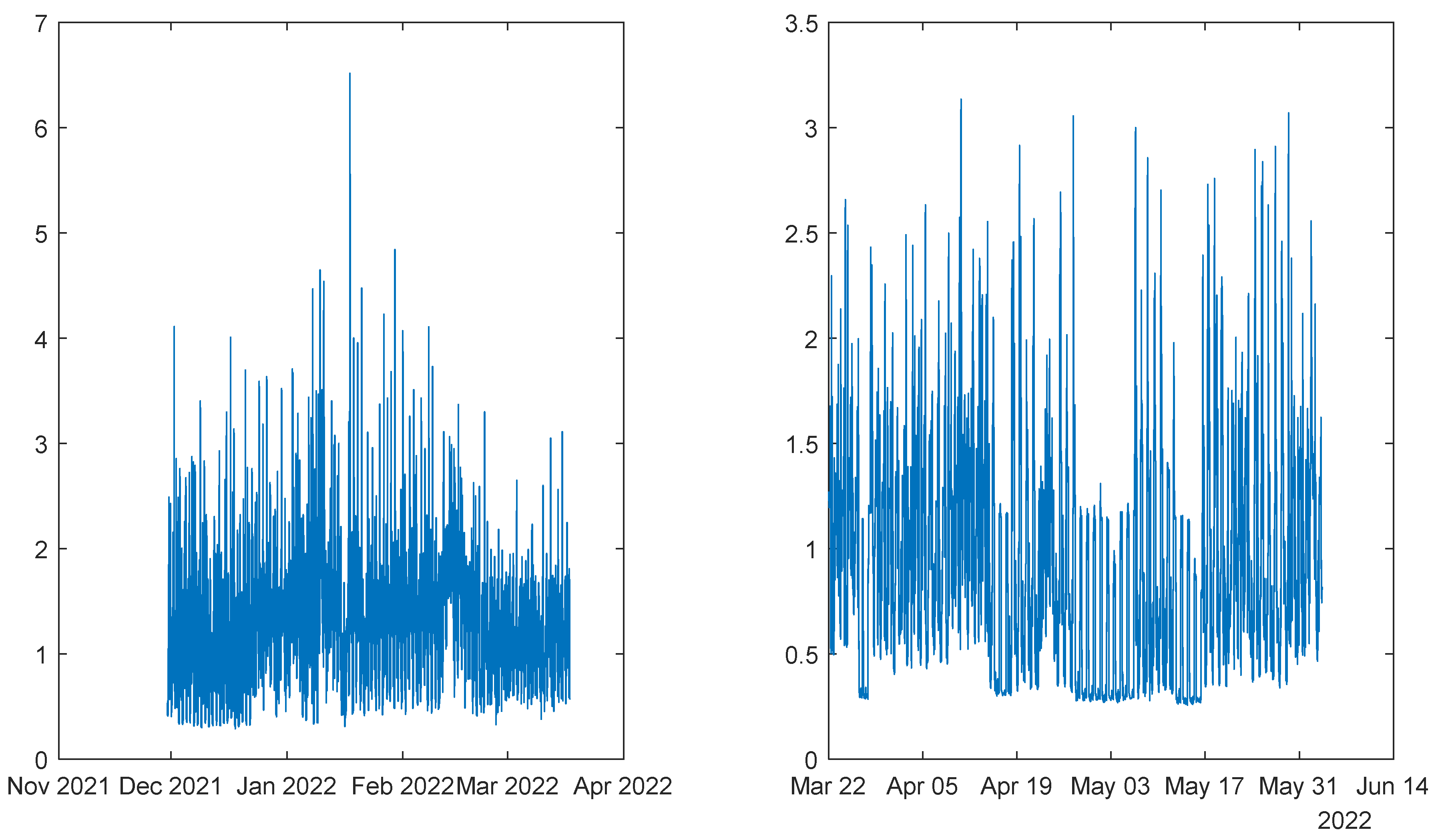
Data acquired from a community of energy situated in Algarve, Portugal, from two time periods were used. Although much smaller sampling intervals were used, the data has been downsampled to intervals of one hour. The first period contained data from 30 November 2021 to 17 March 2022 (2583 samples), and the second period comprised data from 22 March 2022 to 3 Jun 2022 (1762 samples). The houses and the data acquisition system are described in [39,40], and the reader is encouraged to consult these references. The data used here can be freely downloaded at [41].
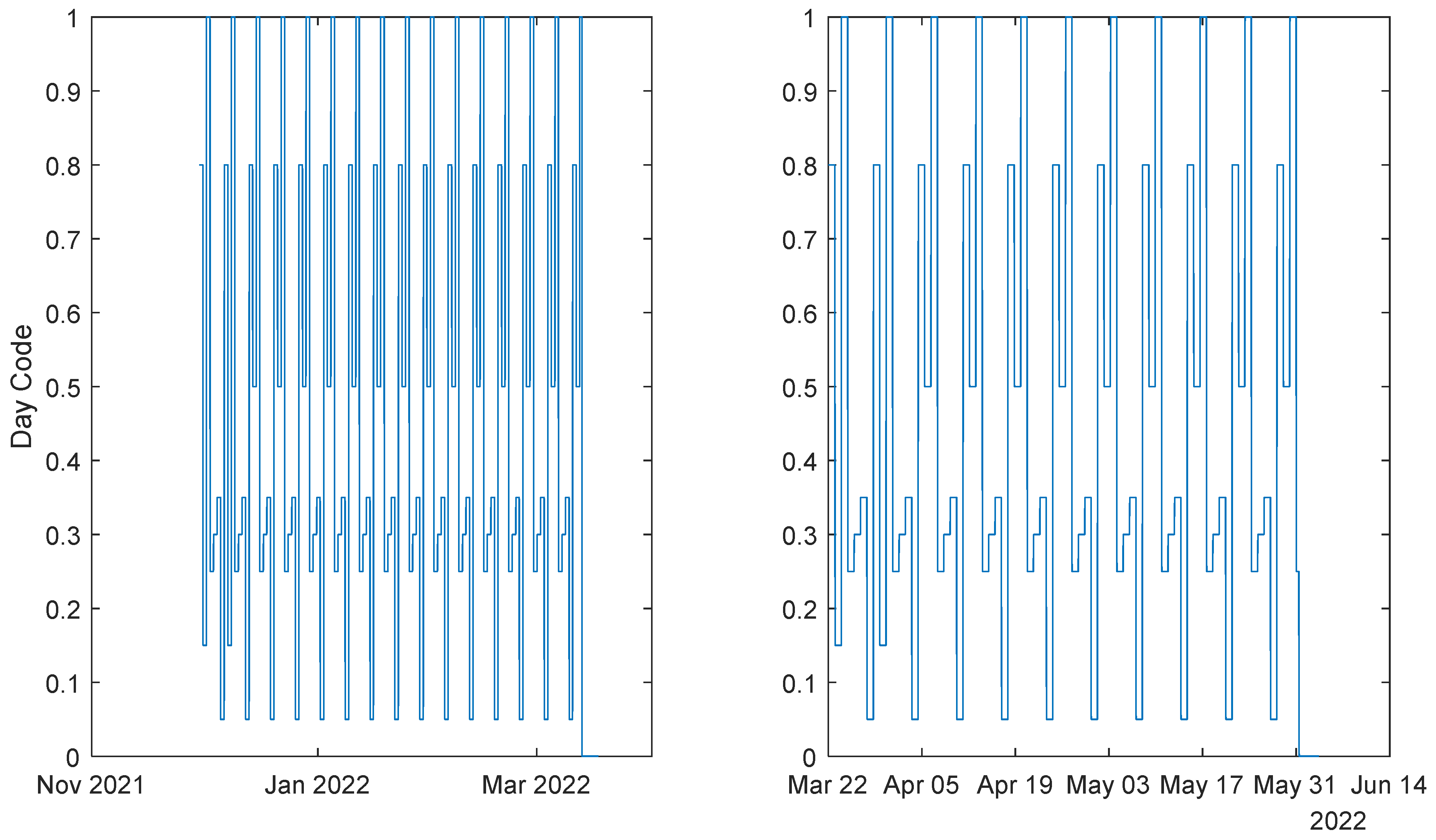
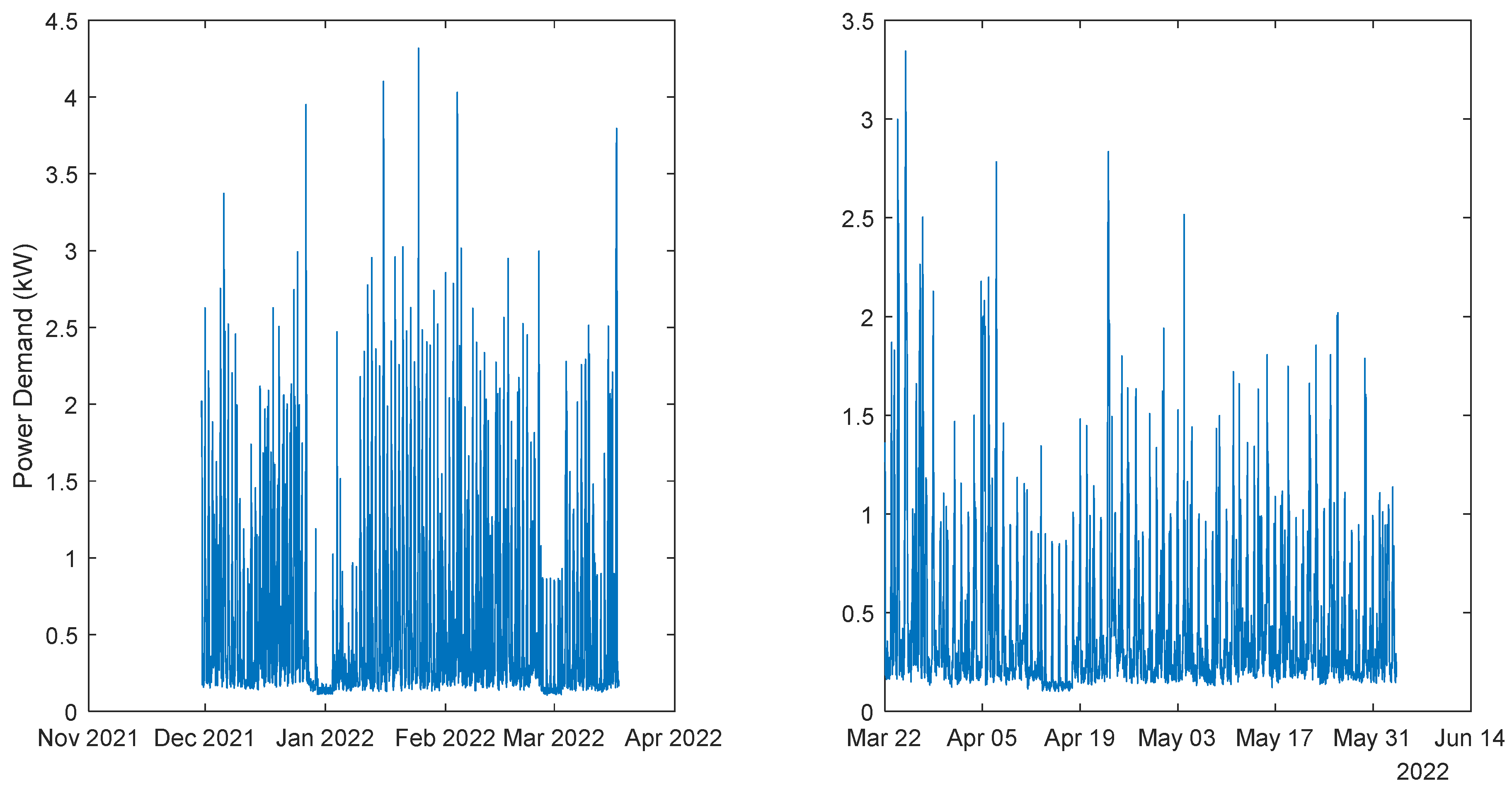
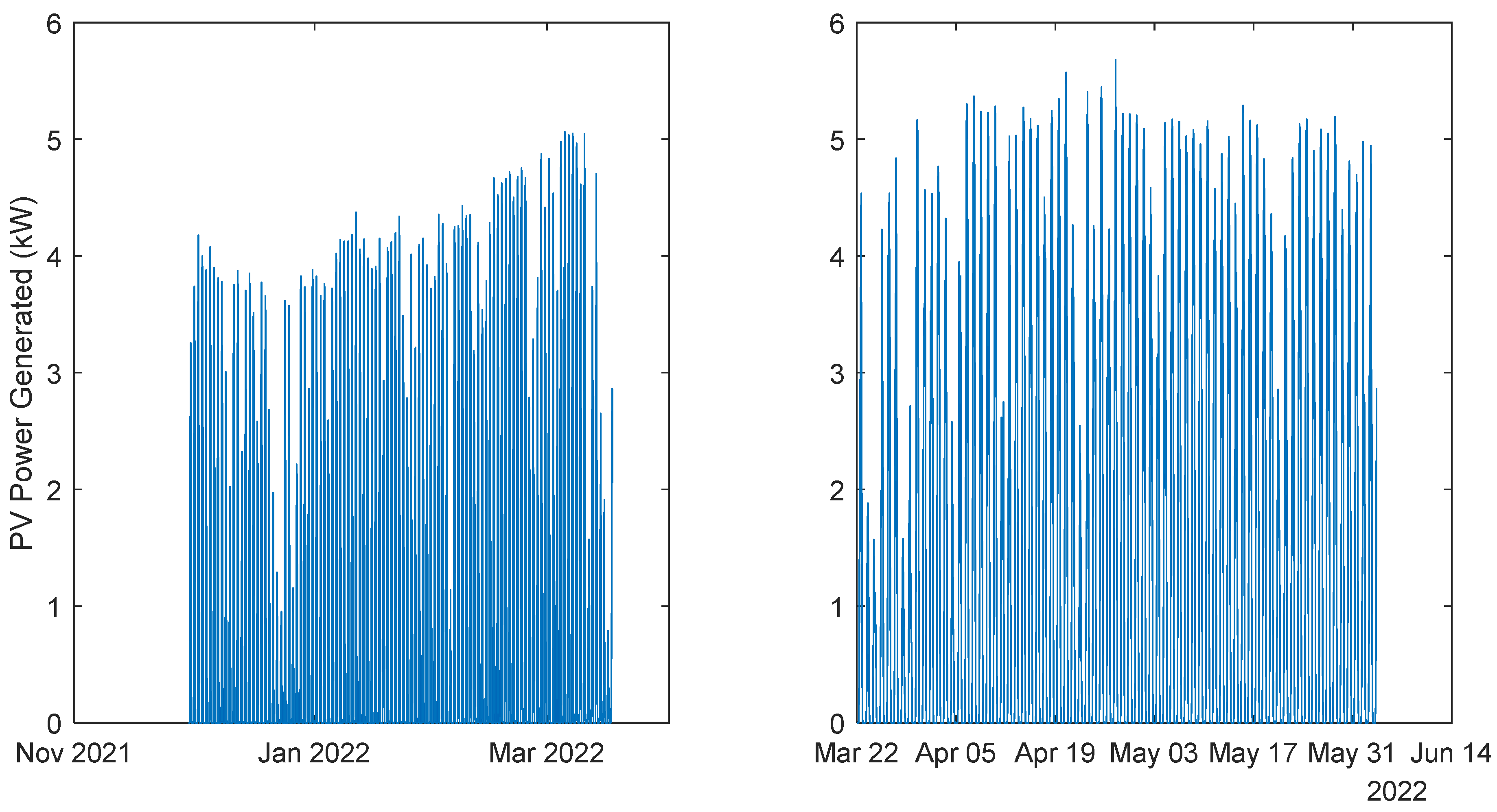
The data that will be used here are weather data, atmospheric air temperature (T) and global solar radiation (R), Power Demand (PD), and PV Power generated (PG). Another feature that is going to be used is a codification for the type of day (DE), characterizing each day as week or weekend days and the occurrence and severity of holidays based on the day they occur, as may be consulted in [11,42].
To be able to help the aggregator regarding the needs of purchasing/selling electricity from/to the market, during the sample related to the period between 11 h–12 h each day, there is the need to forecast the future community power demand and power generated related with the next day, i.e., from 0 to 24 h, in intervals of 1 h. The former can be modeled as an ensemble of NARX models, that for house h in the community will be denoted as:
P ˘ k + 1 | k , h D = M ˘ h D P ¯ k , h D , T ¯ k , C o d e k
The use of the symbol   ͞   in (46) represents a set of delays of the variable. As four houses will be considered in the community, four different ensemble models can be used, and the summation of their outputs can be used to determine the predictive power demand of the community:
P ˘ k + 1 | k , A l l D = h = 1 4 P ˘ k , h D
An alternative is to employ only one ensemble model, using the sum of the four demands:
P ˘ k + 1 | k , C o m D = M ˘ C o m D h = 1 4 P ¯ k , h D , T ¯ k , C o d e k
The power generated can also be modeled as a NARX model:
P ˘ k + 1 | k G = M ˘ G P ¯ k G , R ¯ k , T ¯ k
As can be seen, air temperature is used as an exogenous variable in (46), (48), and (49), and solar radiation in (49). This means that the evolution of these variables should also be predicted. Solar radiation can be modeled as an ensemble of NAR models:
R ^ k + 1 | k = M ˘ R R ¯ k
The air temperature is modeled as:
T ˘ k + 1 | k = M ˘ T T ¯ k
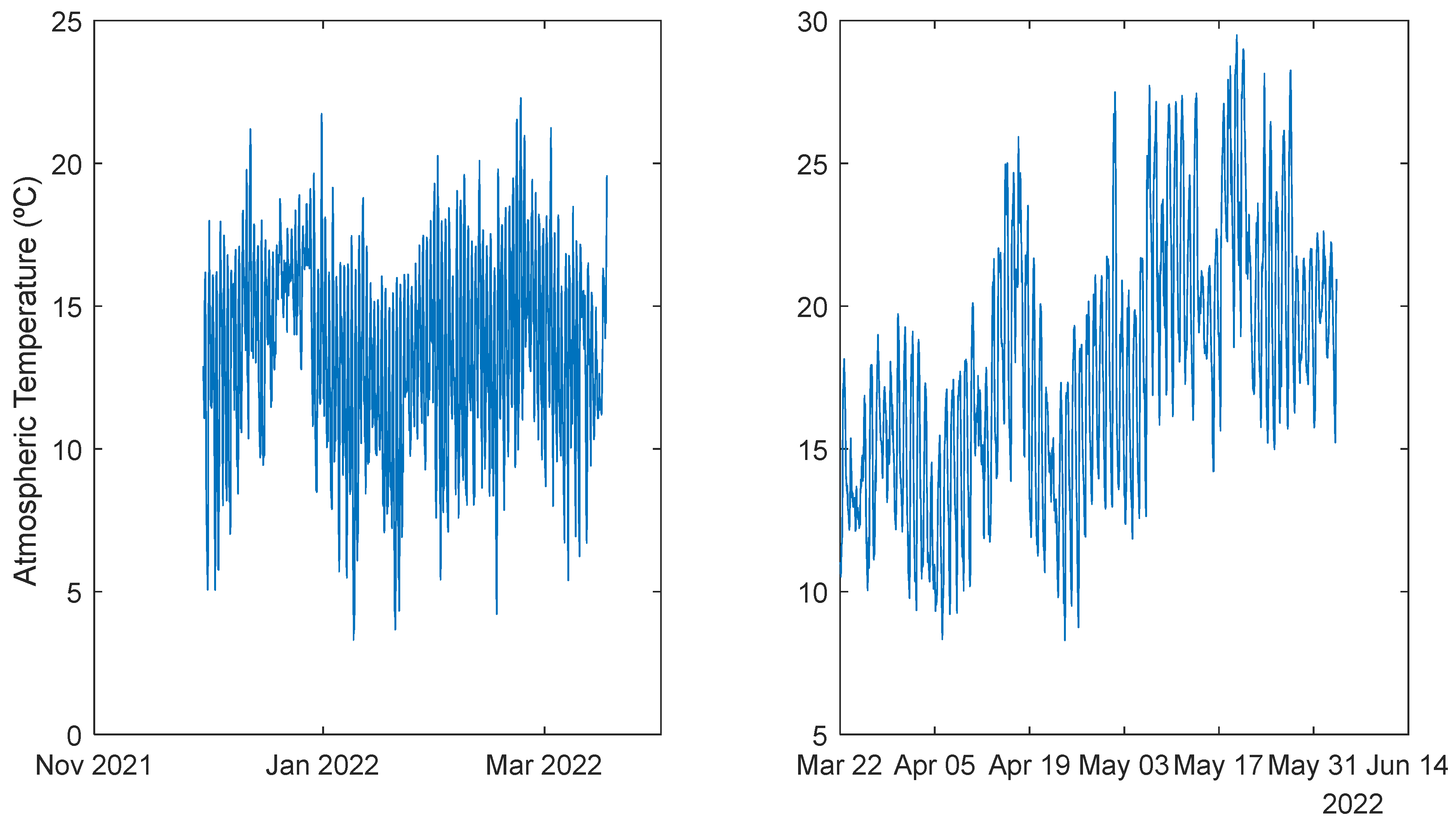
The data employed for the two periods are illustrated in Figure 2, Figure 3, Figure 4, Figure 5, Figure 6, Figure 7, Figure 8 and Figure 9.
As described earlier, several models will be designed: four power demand models, one for each house and an additional one for the community, two weather models, and one power generated model. The procedure described in Figure 1 and detailed in [28] is followed. Two executions of MOGA were performed for each model ensemble, the first minimizing ρ t r , ρ t e , #(v), and ρ s i m P H ; in the second run, some objectives were set as goals.
For all problems, the parameterization of MOGA was:
  • Prediction Horizon: thirty-six steps (36 h).
  • Number of neuros: n n 2 20 ;
  • Initial parameter values: OAKM [43];
  • Number of training trials: five, best compromise solution.
  • Termination criterion: early stopping, with a maximum number of iterations of fifty.
  • Number of generations: 100.
  • Population size: 100.
  • Proportion of random emigrants: 0.10.
  • Crossover rate: 0.70.
For the NARX models, the number of possible inputs was from 1 to 30, while for NAR models, the range used was from 1 to 20.
As already mentioned, for each model, two executions of MOGA are performed, the results of the first being analyzed to constrain the objectives and ranges of neurons and inputs of the second execution.
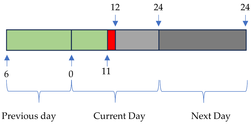
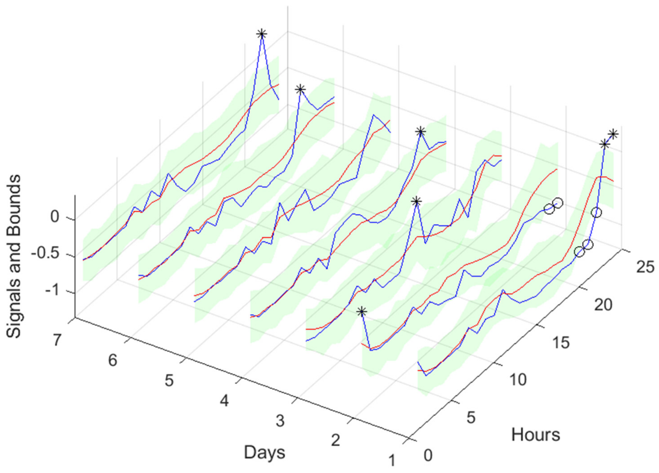
The next figure (Figure 10) illustrates the range of forecasts pretended and the delays employed. Every day, a few minutes before 12, the average power for the period 11–12 is computed. Let us denote the index of this sample by k (in red). Using the delayed average powers of the previous 29 indices [k − 1 … k − 29] (shown in green), we need to forecast the average powers for the next day. Therefore, using a multi-step forecast model, there is the need to forecast 36 steps ahead of values (in cyan), from which only the last 24 steps are required (darker cyan).
The forecasting performance will be assessed using a prediction time series, from 19 January 2022 00:30:00 to 25 January 2022 23:30:00, with 168 samples. All simulations were performed in Matlab, version 9.14.0.2337262 (R2023a) Update 5.

3.2. Solar Radiation Models

Solar Radiation is a NAR model. Table 1 shows statistics corresponding to the mean of the employed performance criteria, averaged over the Prediction Horizon. For this model and for the others, the results are related to the 2nd MOGA execution. Unless explicitly specified, scaled values belonging to the interval [−1 … 1] are employed. This enables a comparison of the performance between different variables. The MAPE value is shown in %.
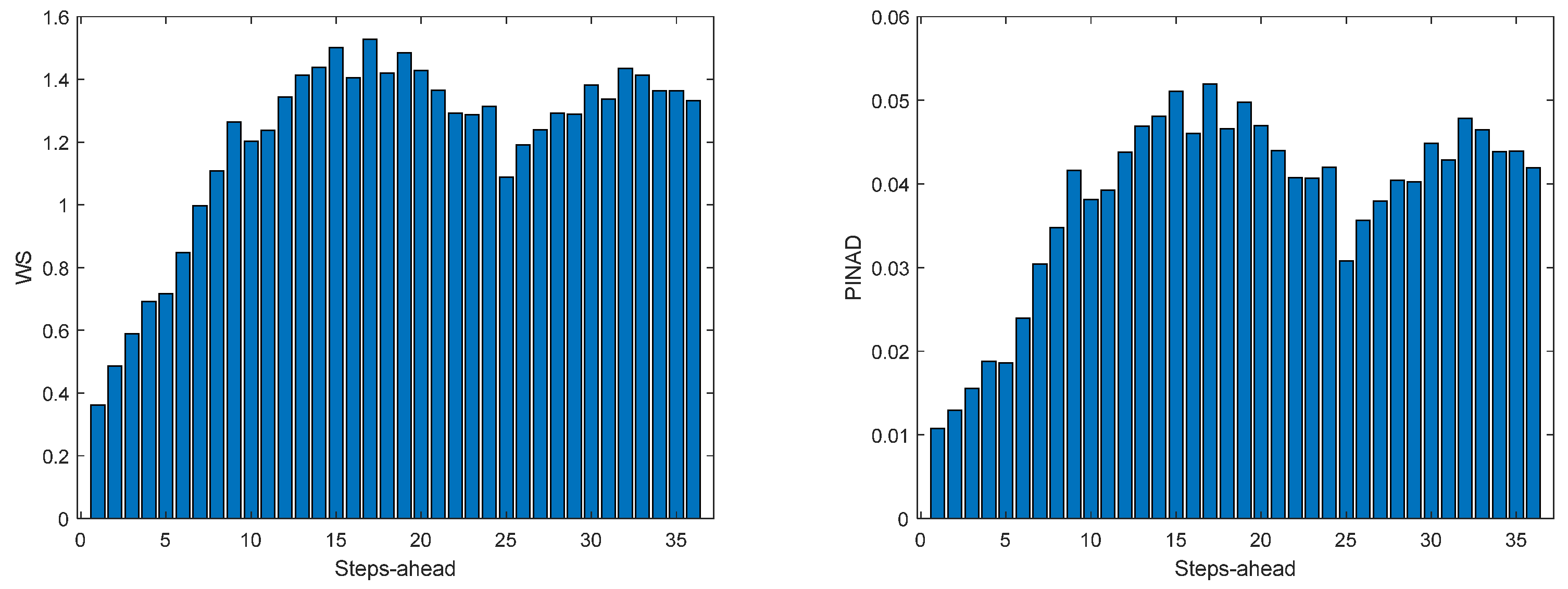
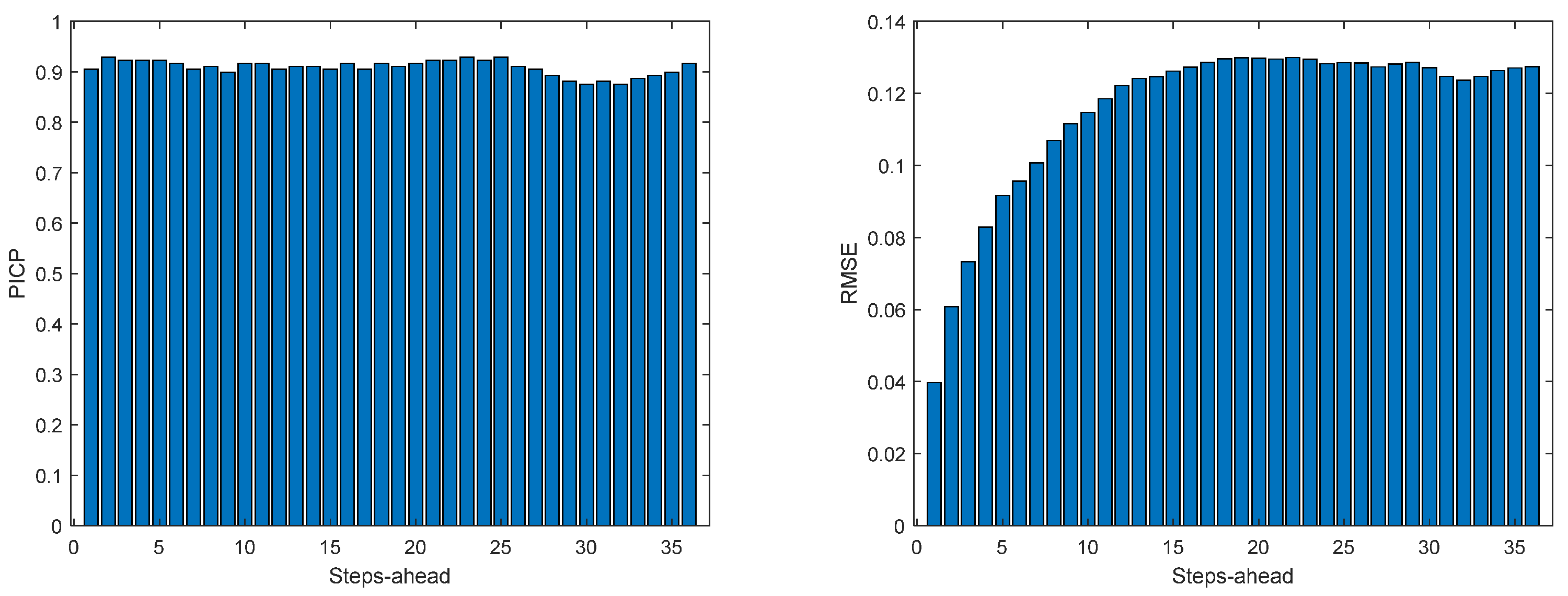
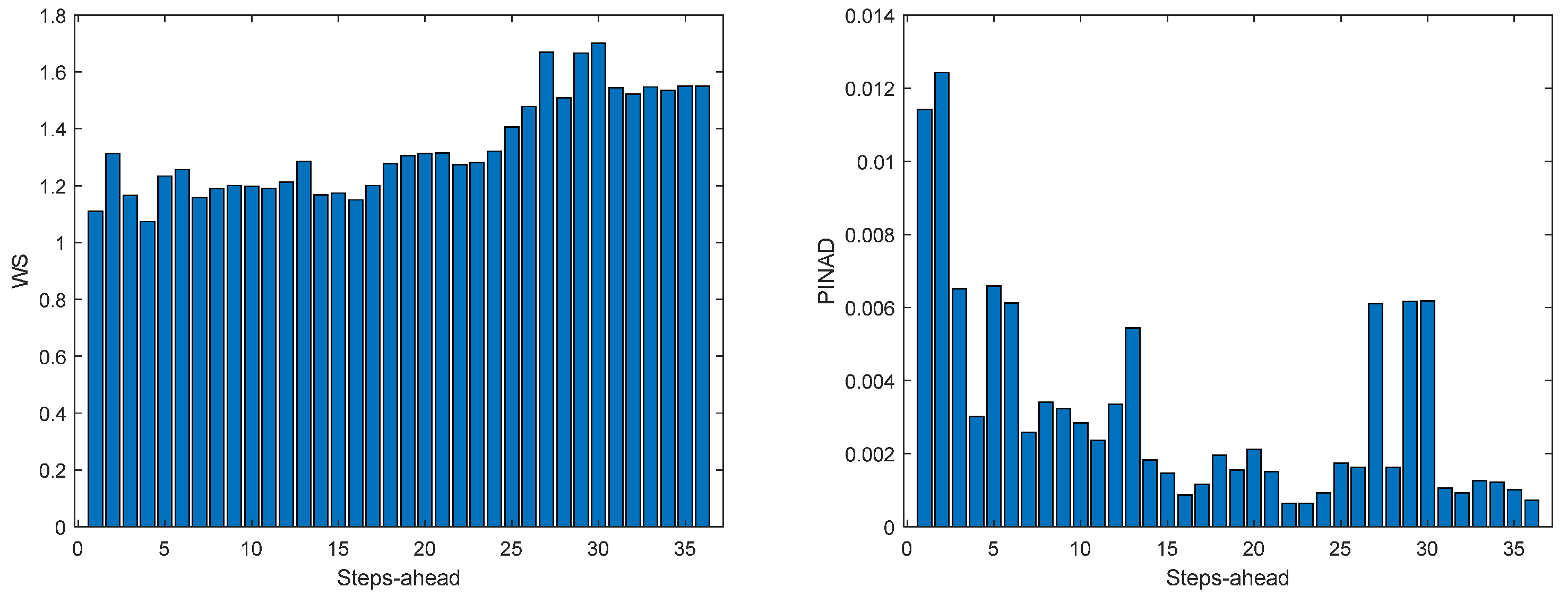
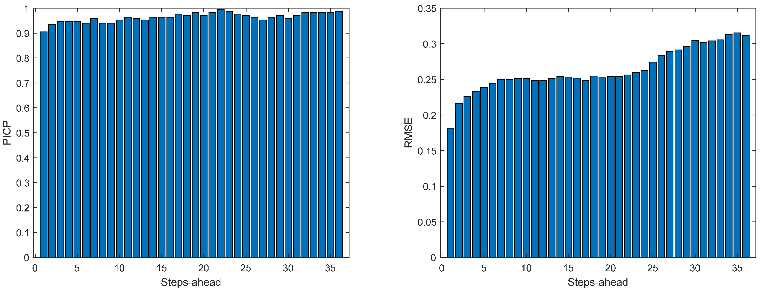
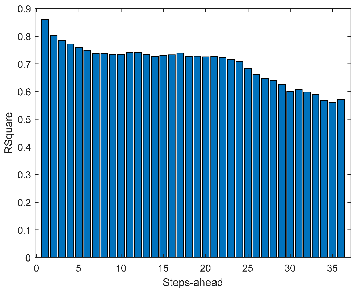
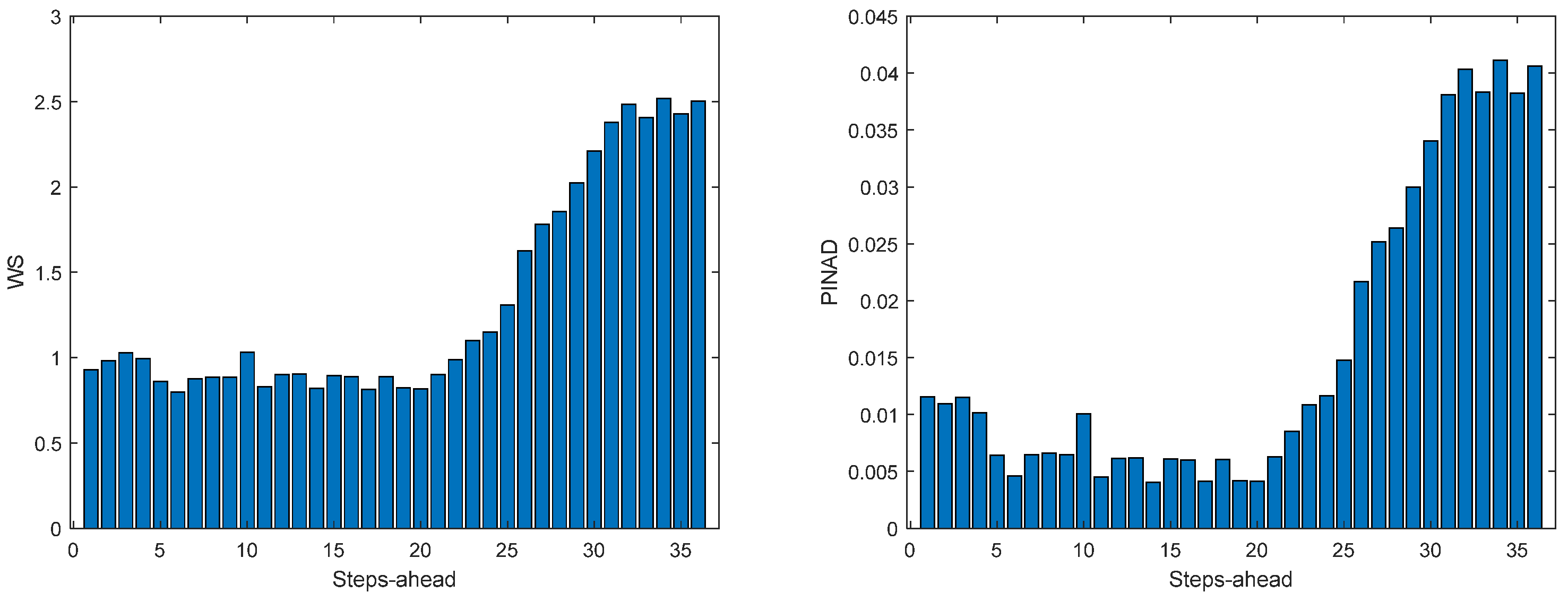
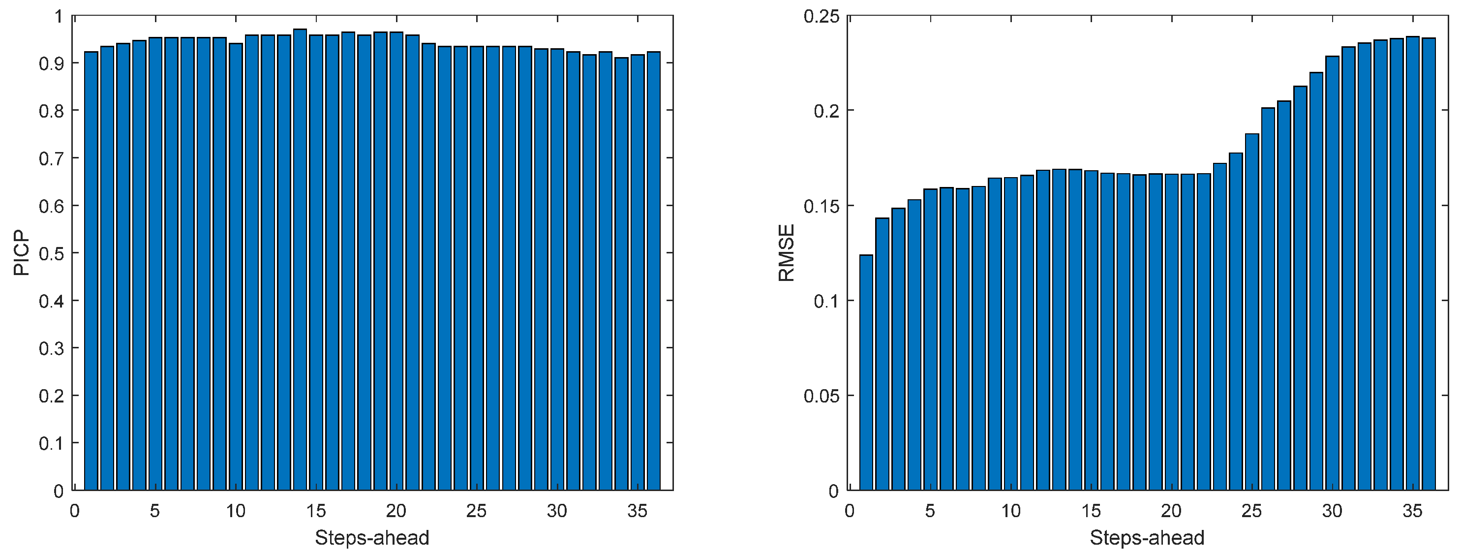
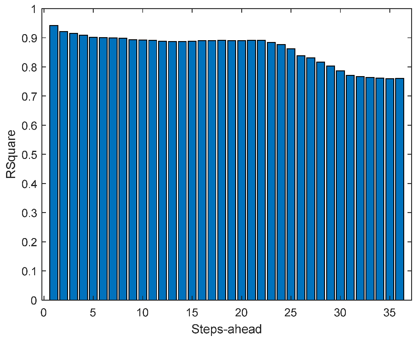
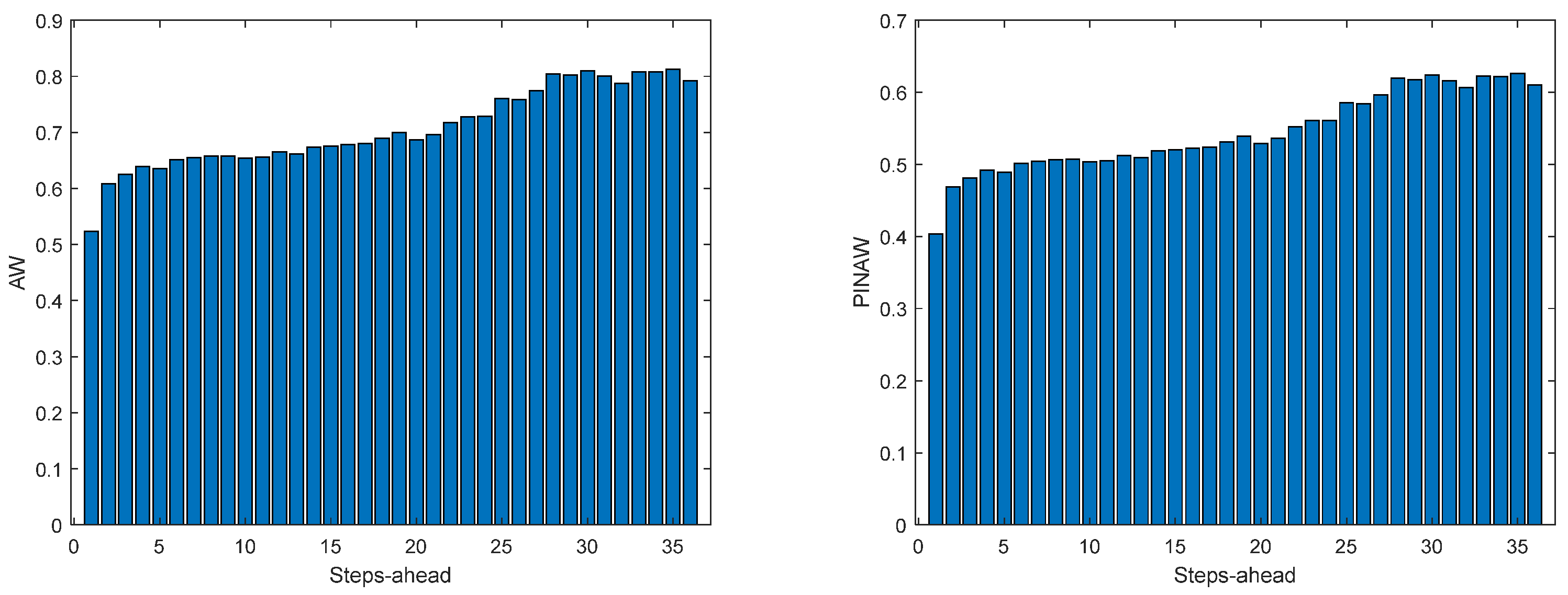
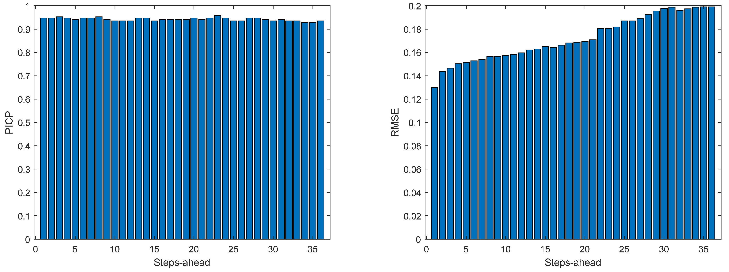
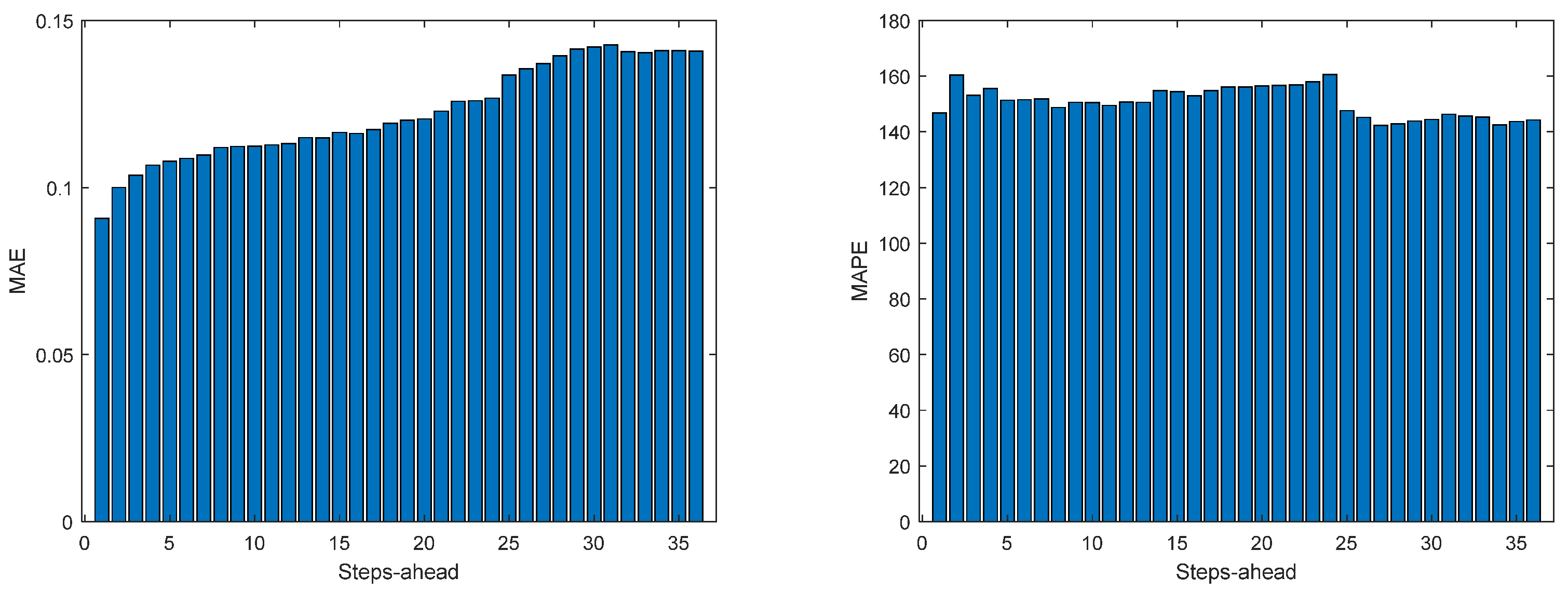
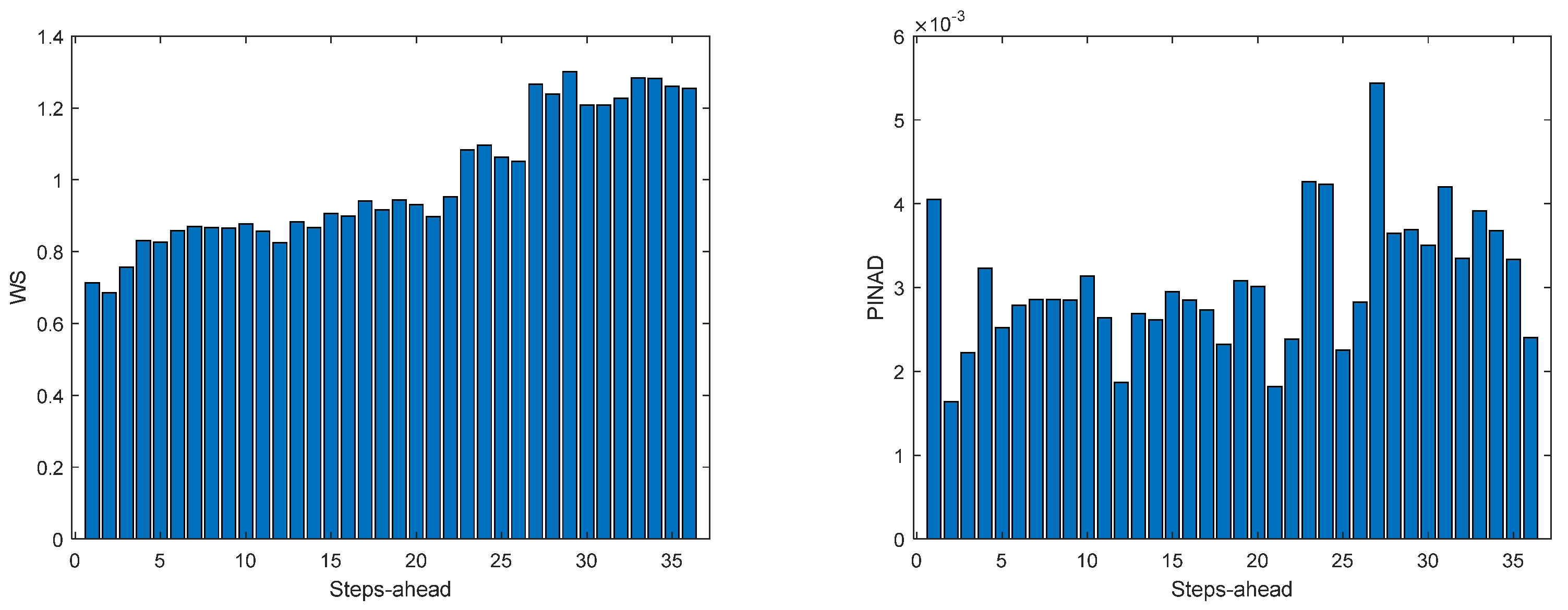
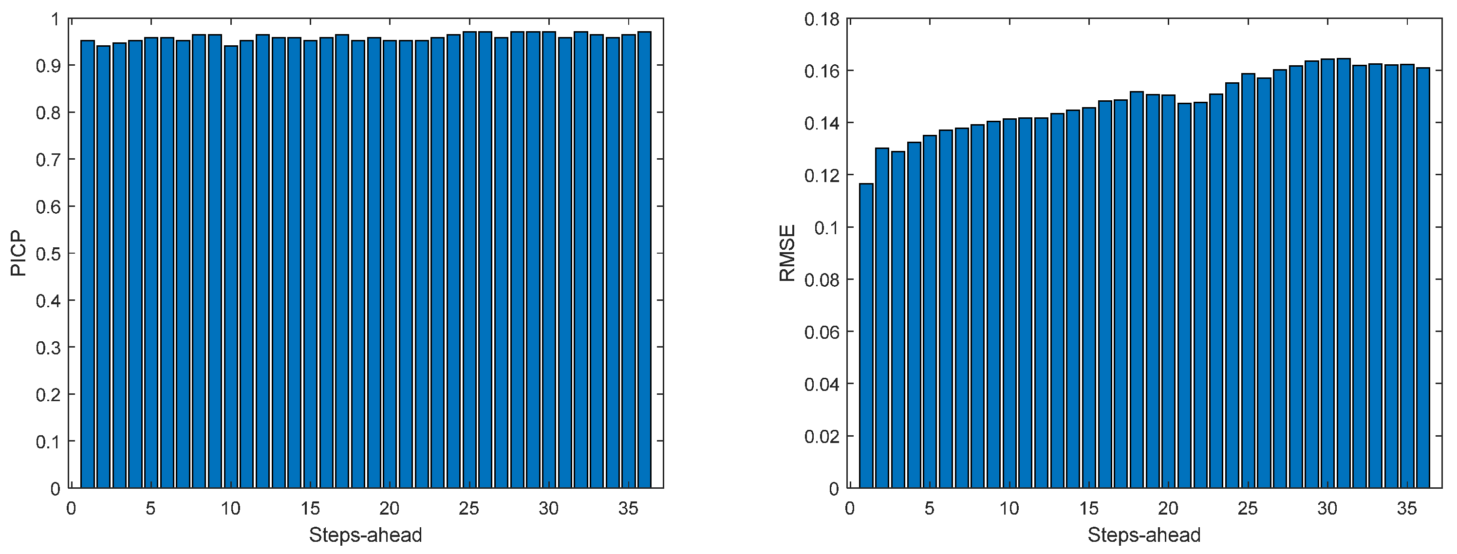
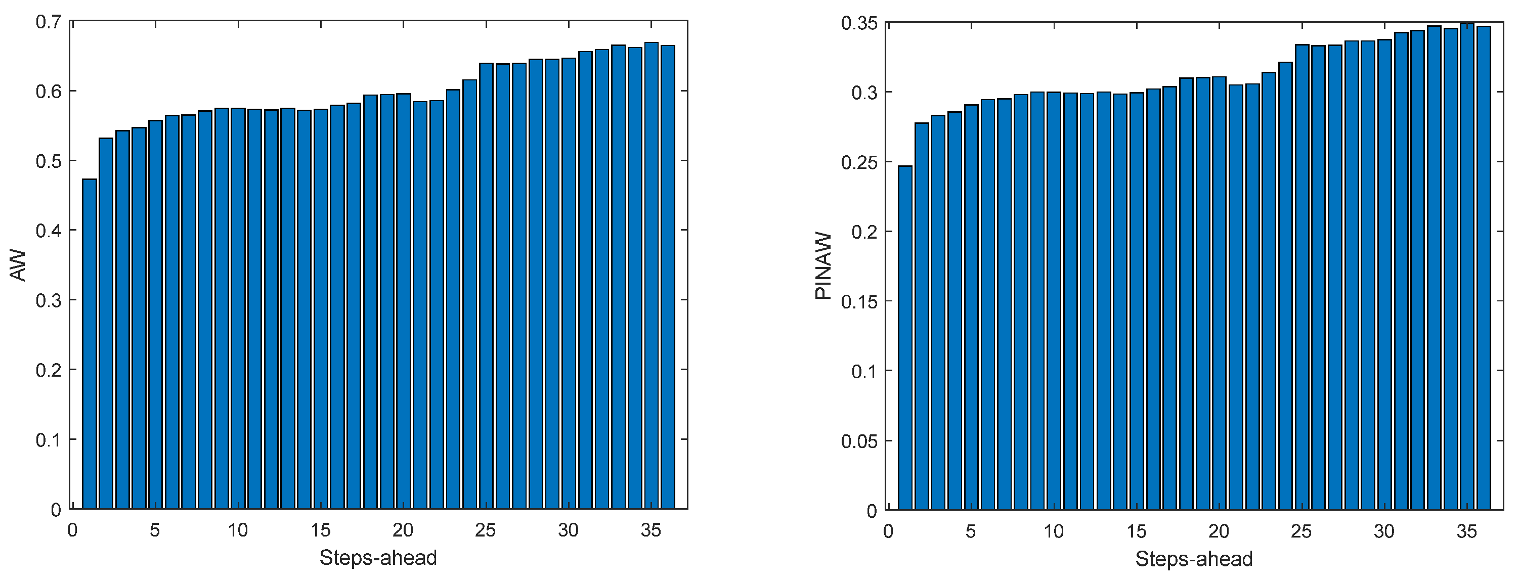
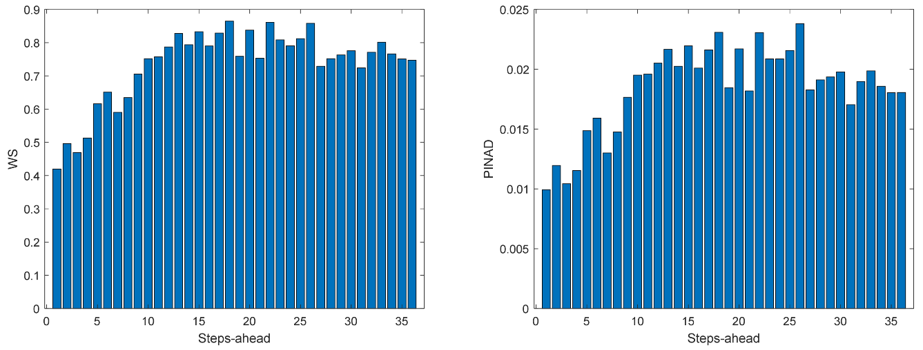
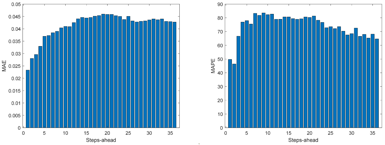
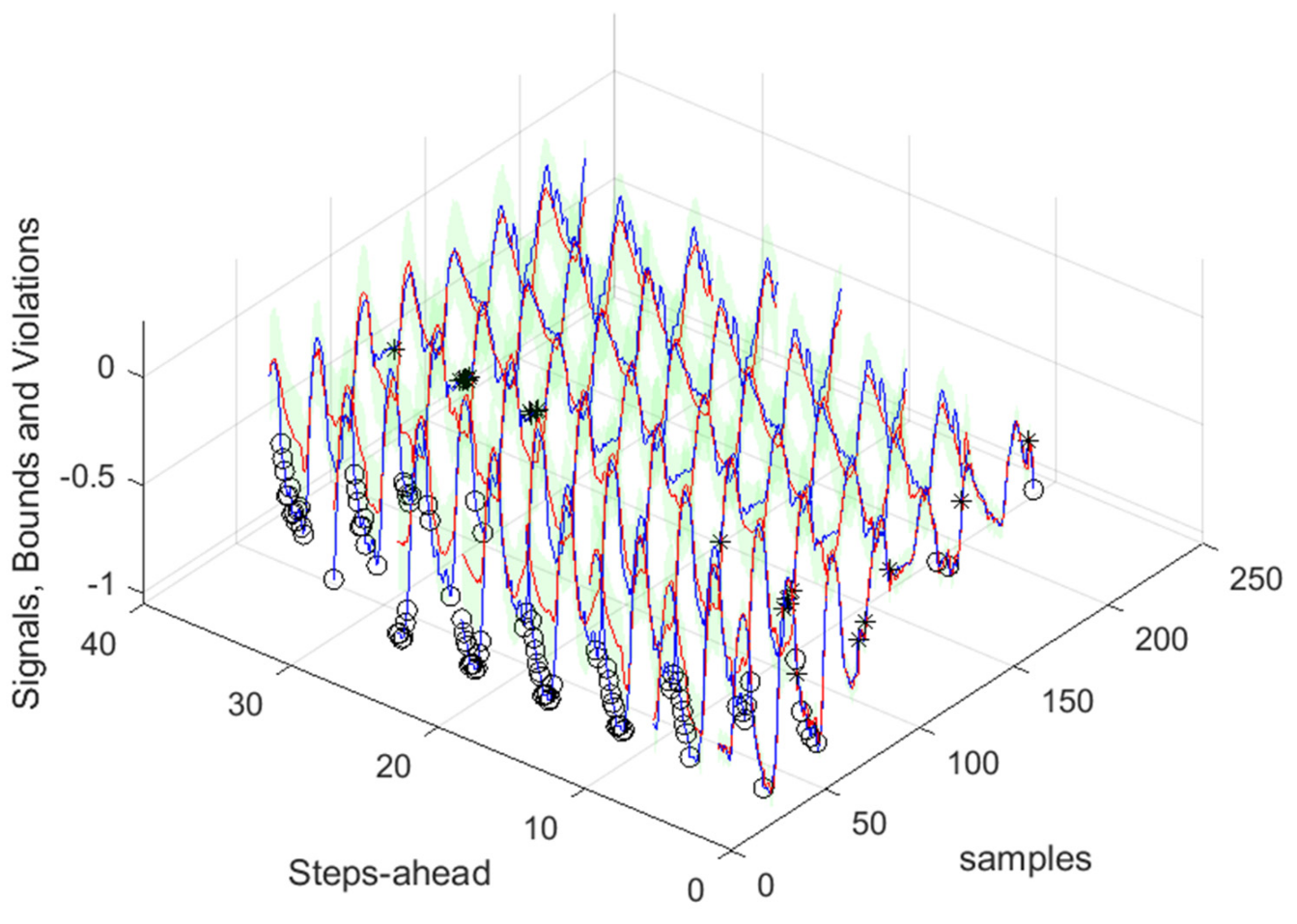
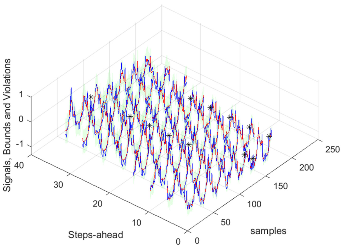
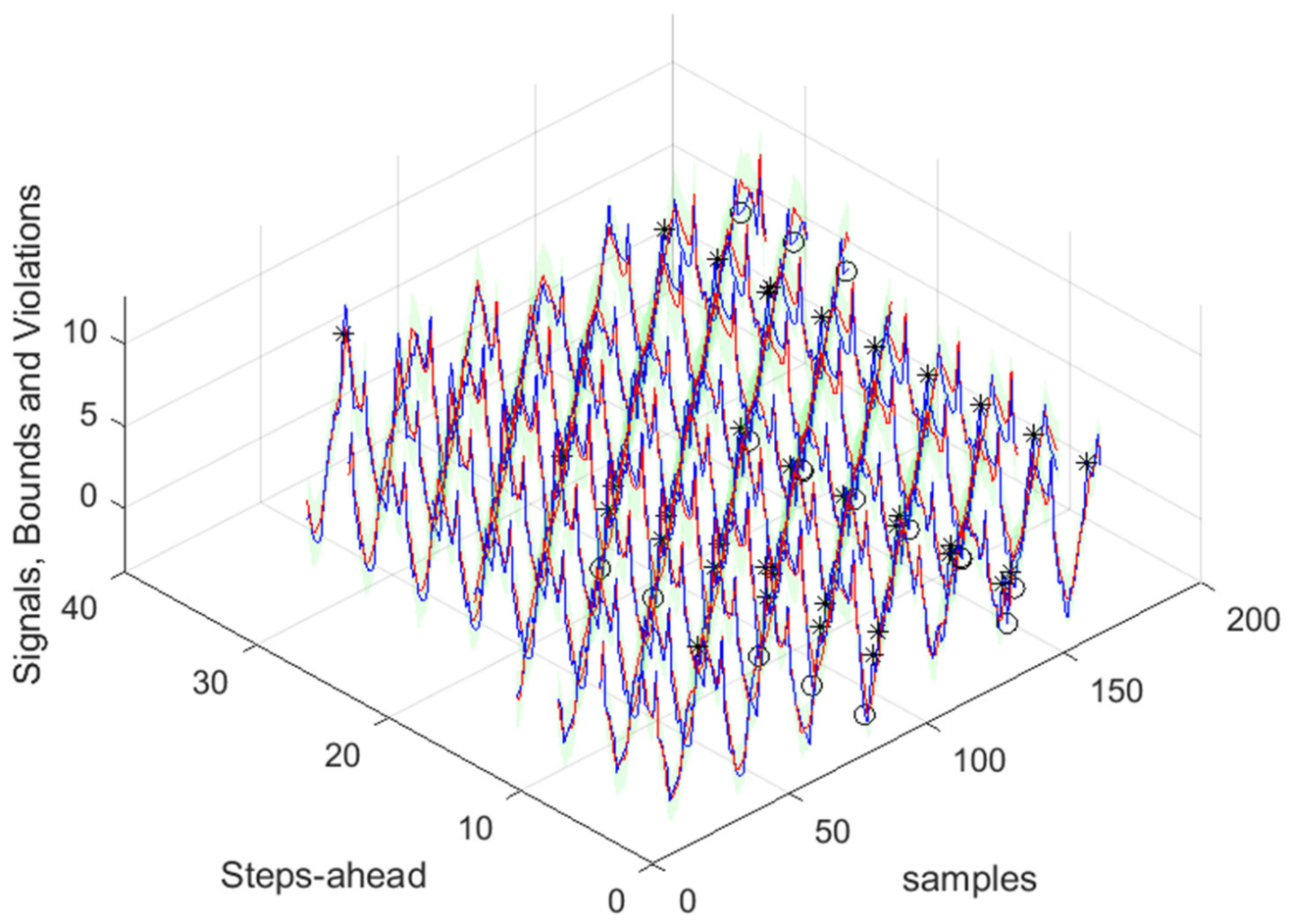
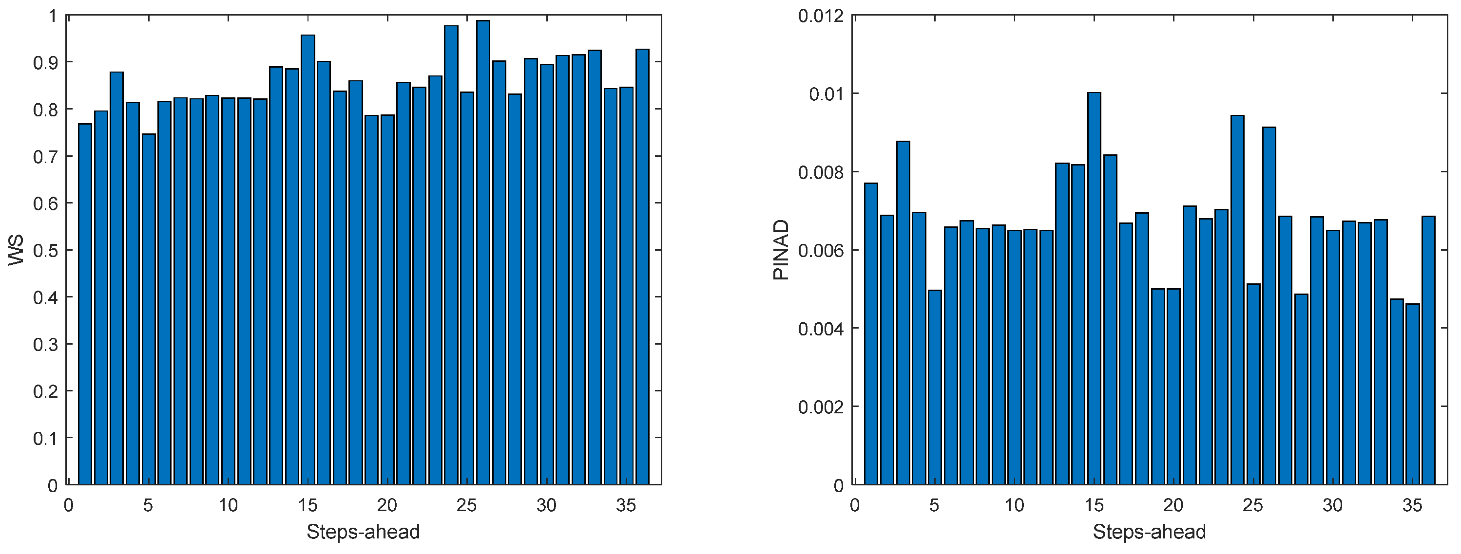
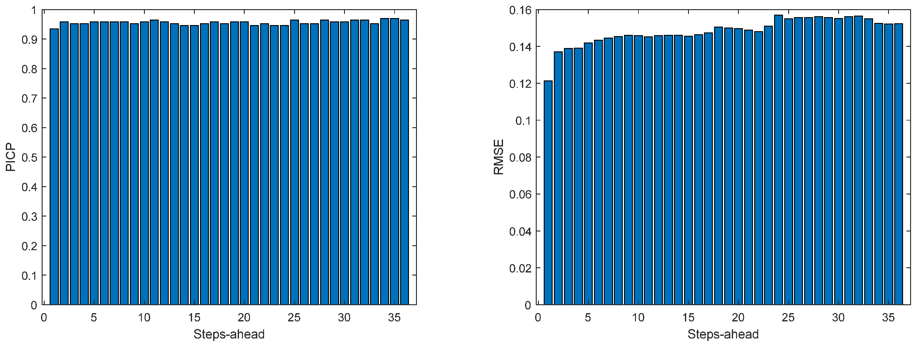
As it can be concluded from analyzing Table 1 and Figure 11, Figure 12, Figure 13, Figure 14, Figure 15, Figure 16, Figure 17 and Figure 18, PICP does not vary significantly along PH and is always greater than 0.9. The other robustness measures increase along the prediction horizon but not significantly. Comparing AW and PINAW, they are related by a scale factor corresponding to the range of the forecasted solar radiation along PH, which remains nearly constant. Although the number of bound violations remains nearly constant over PH (please see PICP—Figure 13 left), the range of the violations changes with each step ahead. This can be confirmed by PINAD evolution (Figure 12 right) and by the Winkler score evolution (Figure 13 left), which penalizes twenty times the magnitude of the violations.
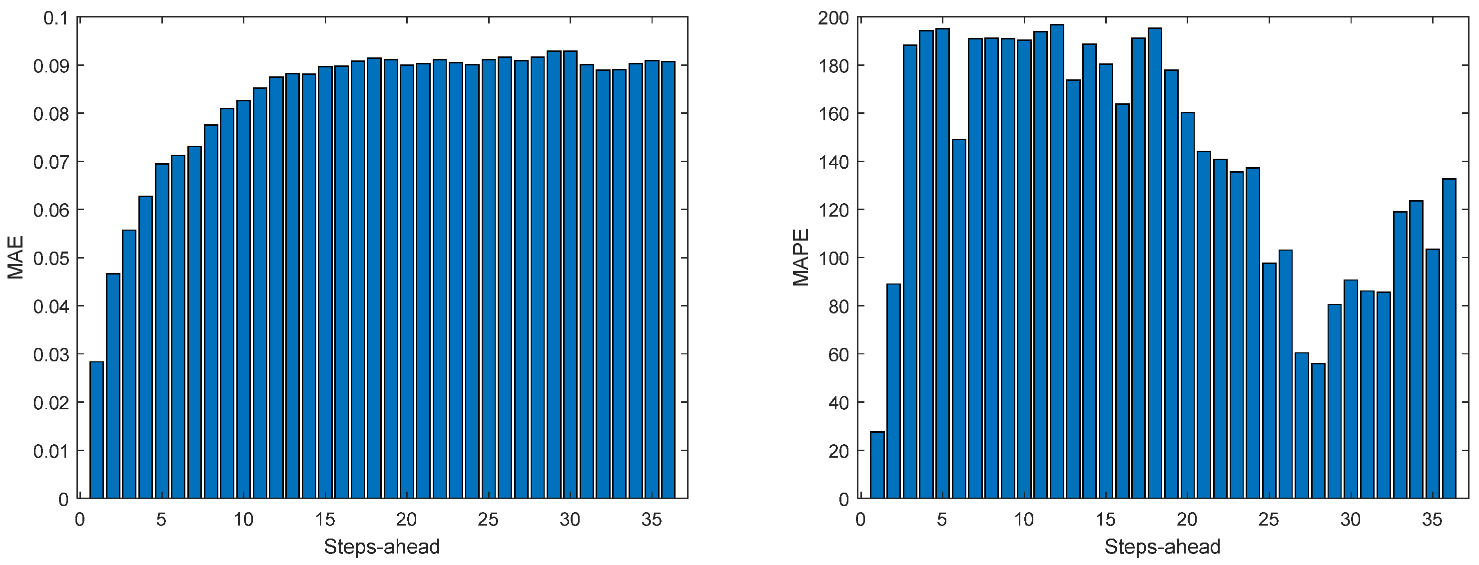
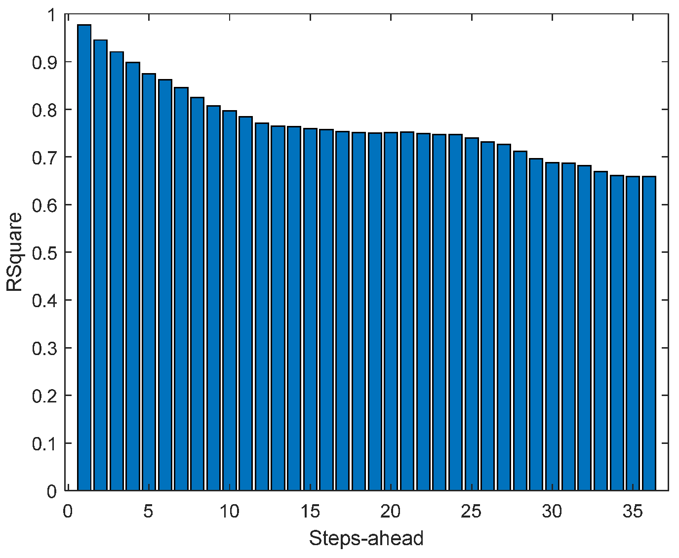
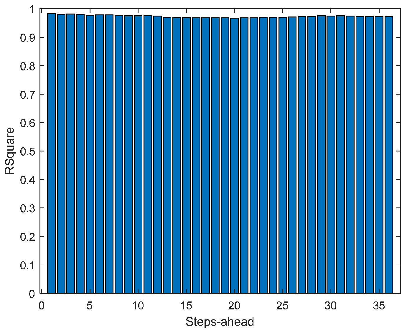
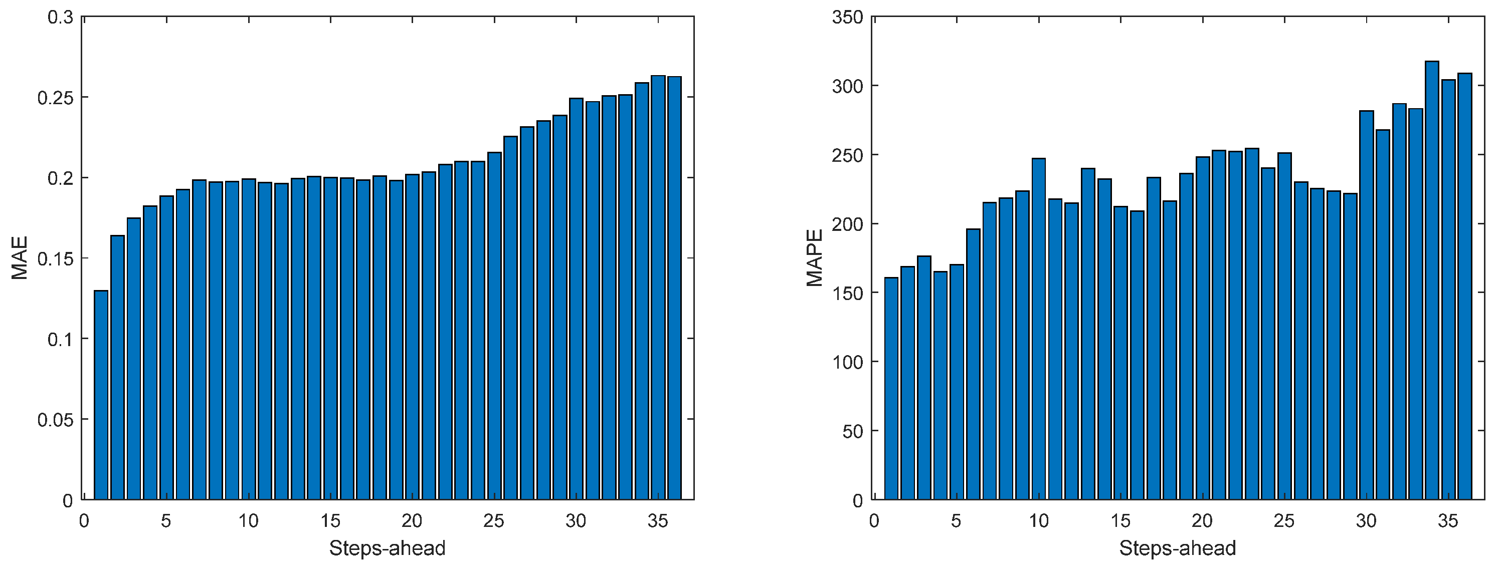
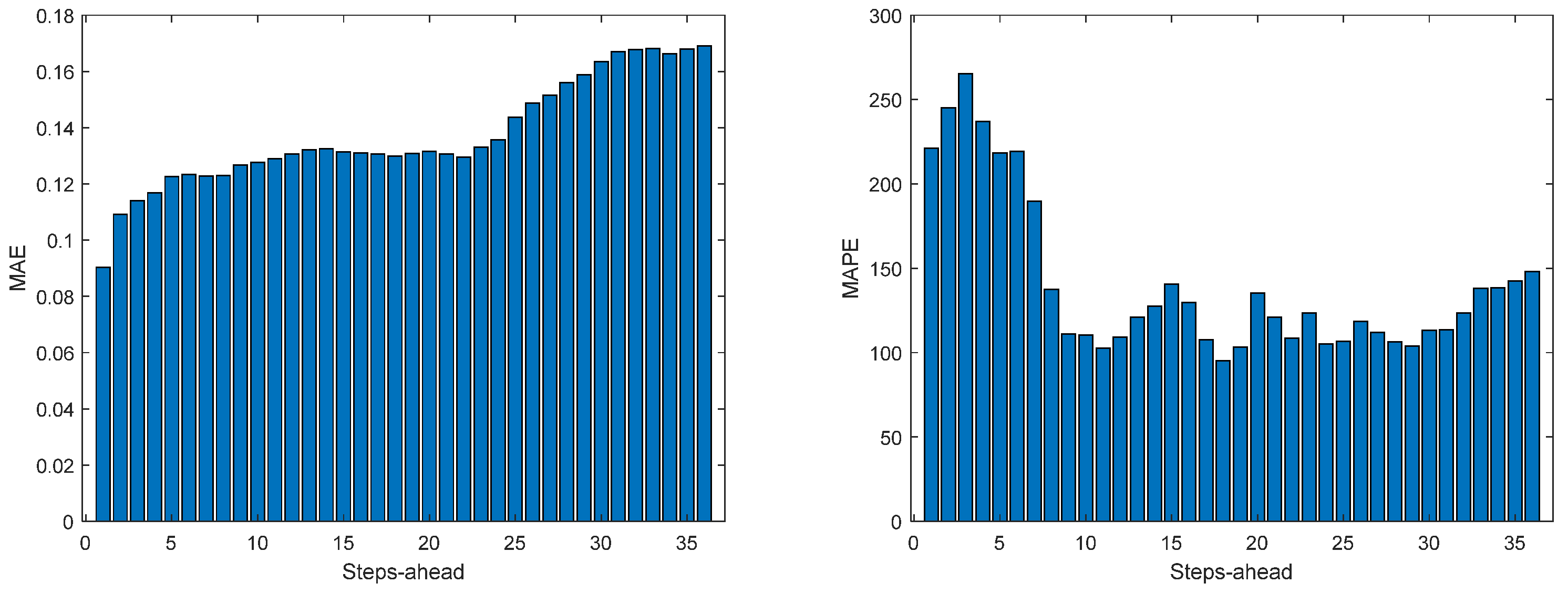
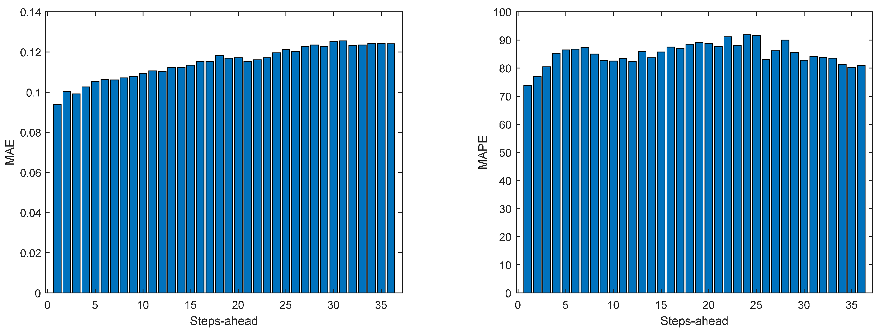
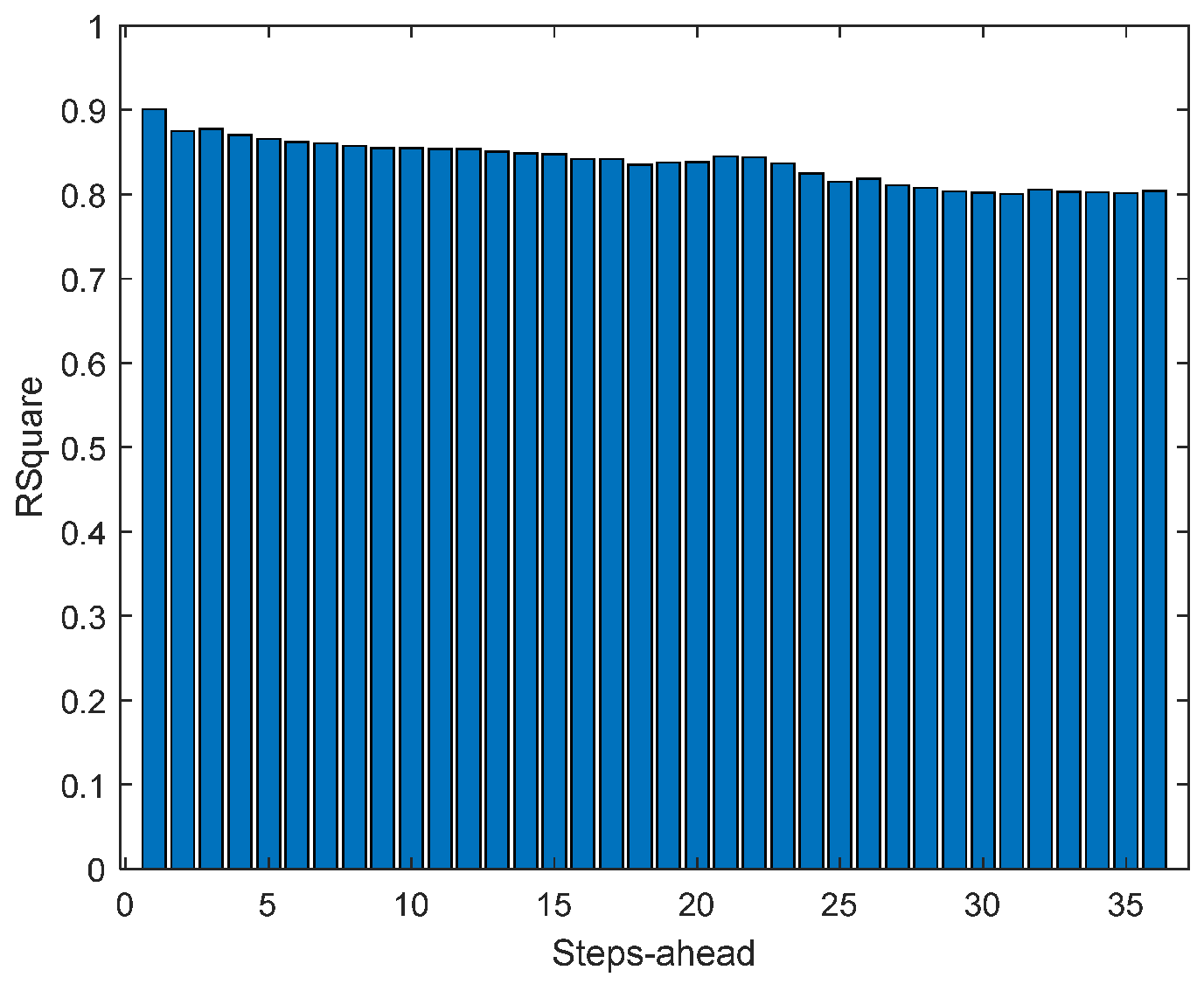
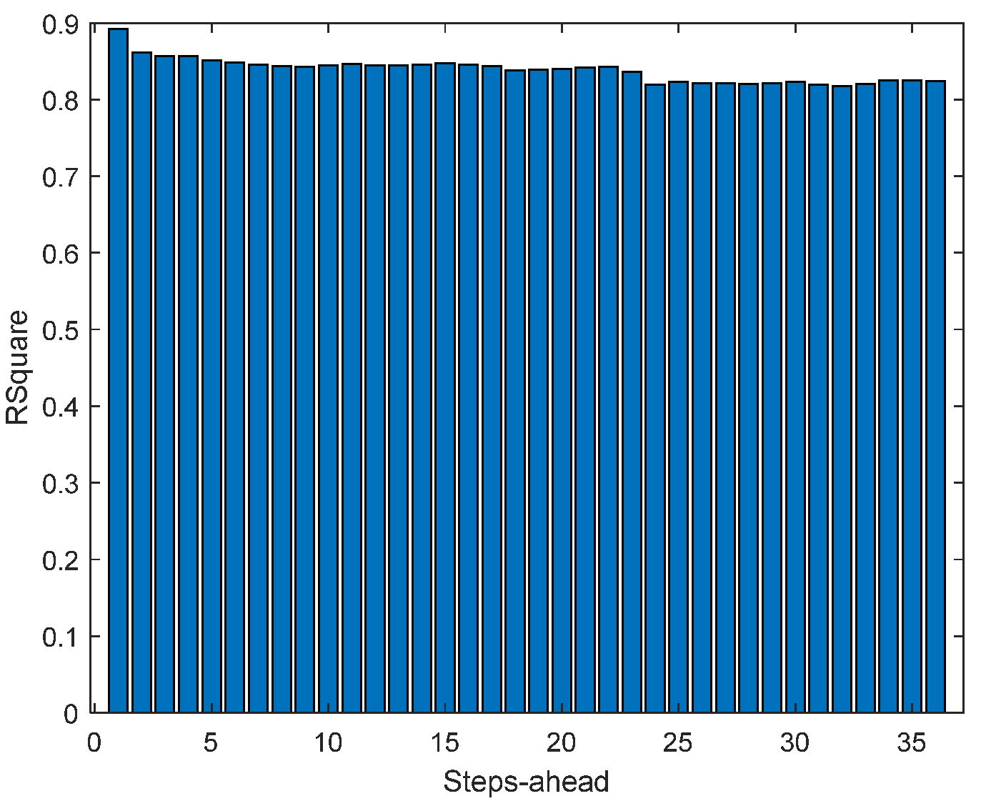
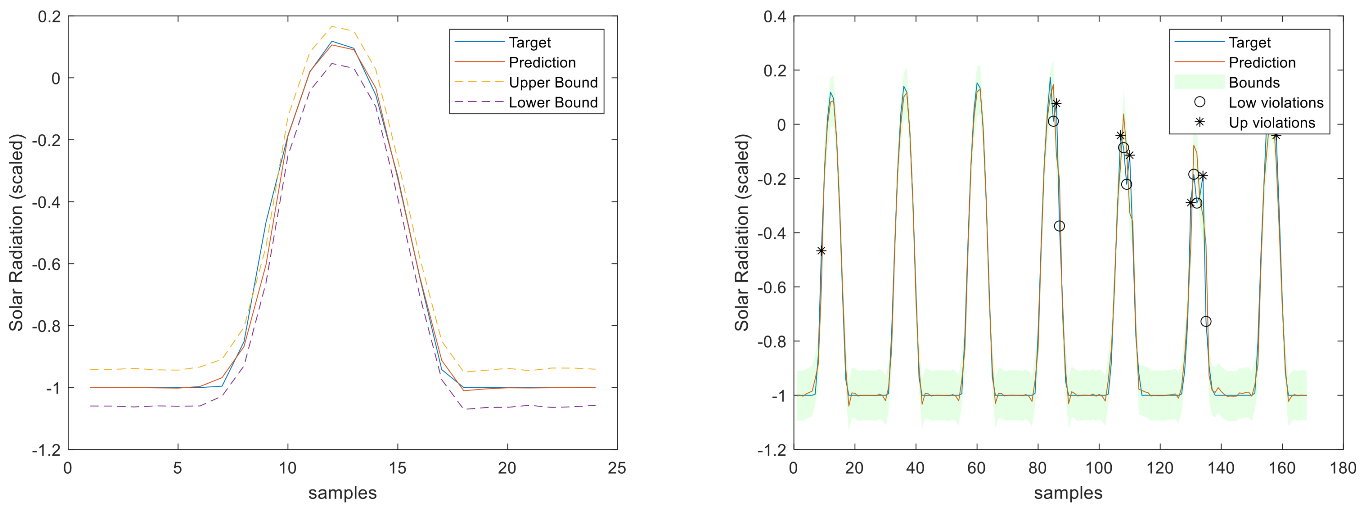
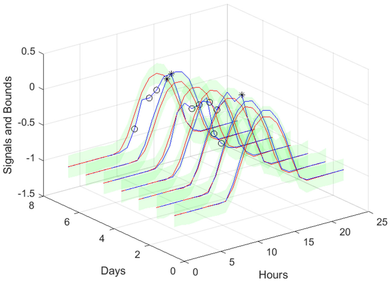
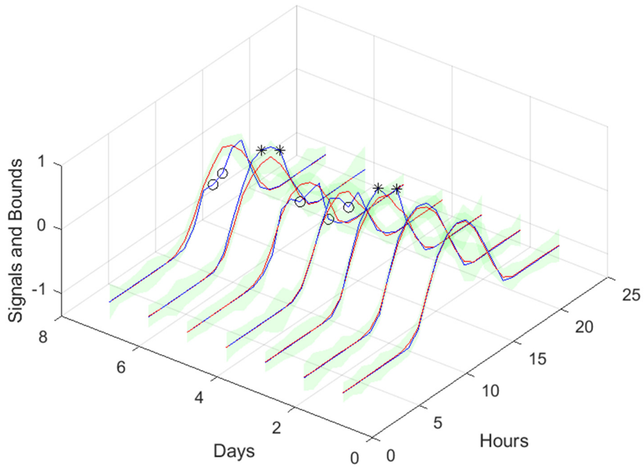
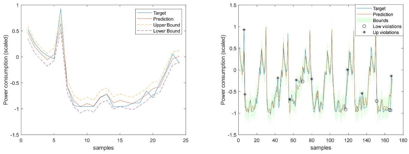
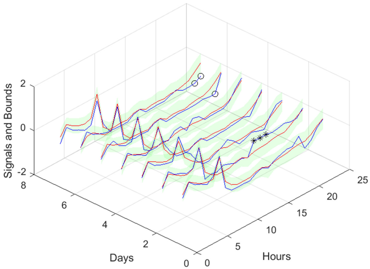
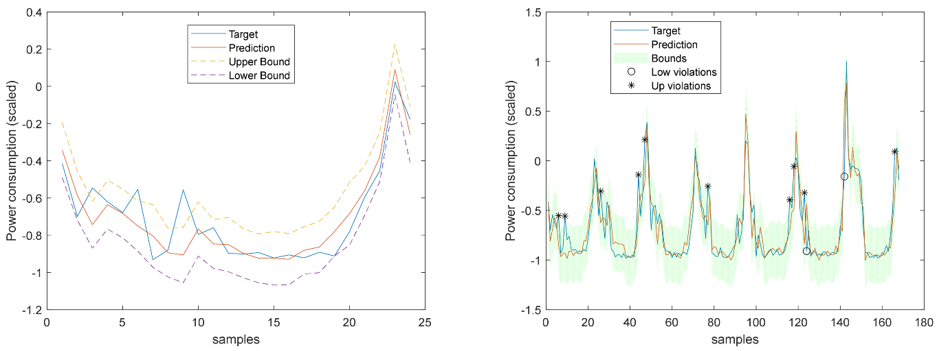
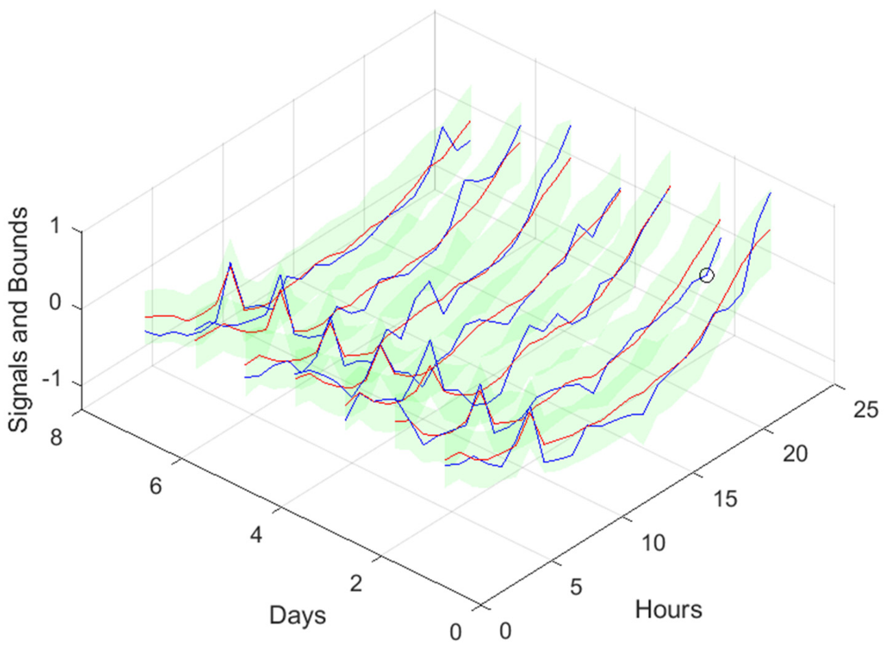
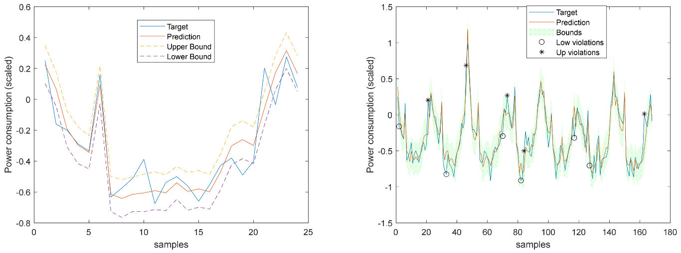
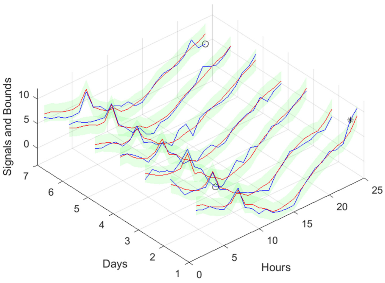
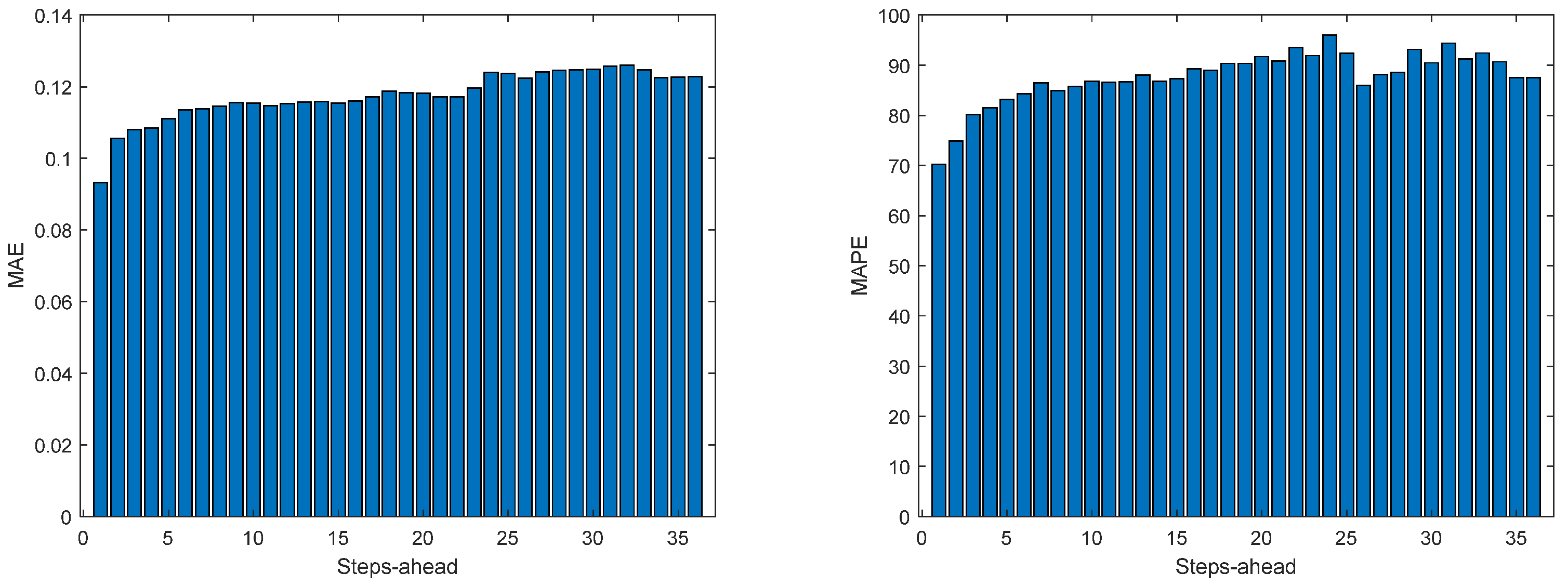
The RMSE, MAE, and MAPE also change along PH, typically increasing with the steps ahead. However, this increase is not high and even sometimes decreases. Analyzing the evolution of the R2, we can see that an excellent fit is obtained and maintained throughout the PH. This can also be seen in Figure 16, left and right. The right figure enables us to confirm that excellent performance is maintained through the PH, both in terms of fitting as well as prediction bounds and violations. Finally, Figure 18 focuses on our goal, which is to inspect the day-ahead predictions obtained with data obtained up to 12 h the day before. As can be seen, only twelve small violations were verified, which resulted in a PICP of 93% in those 7 days.

3.3. Atmospheric Air Temperature Models

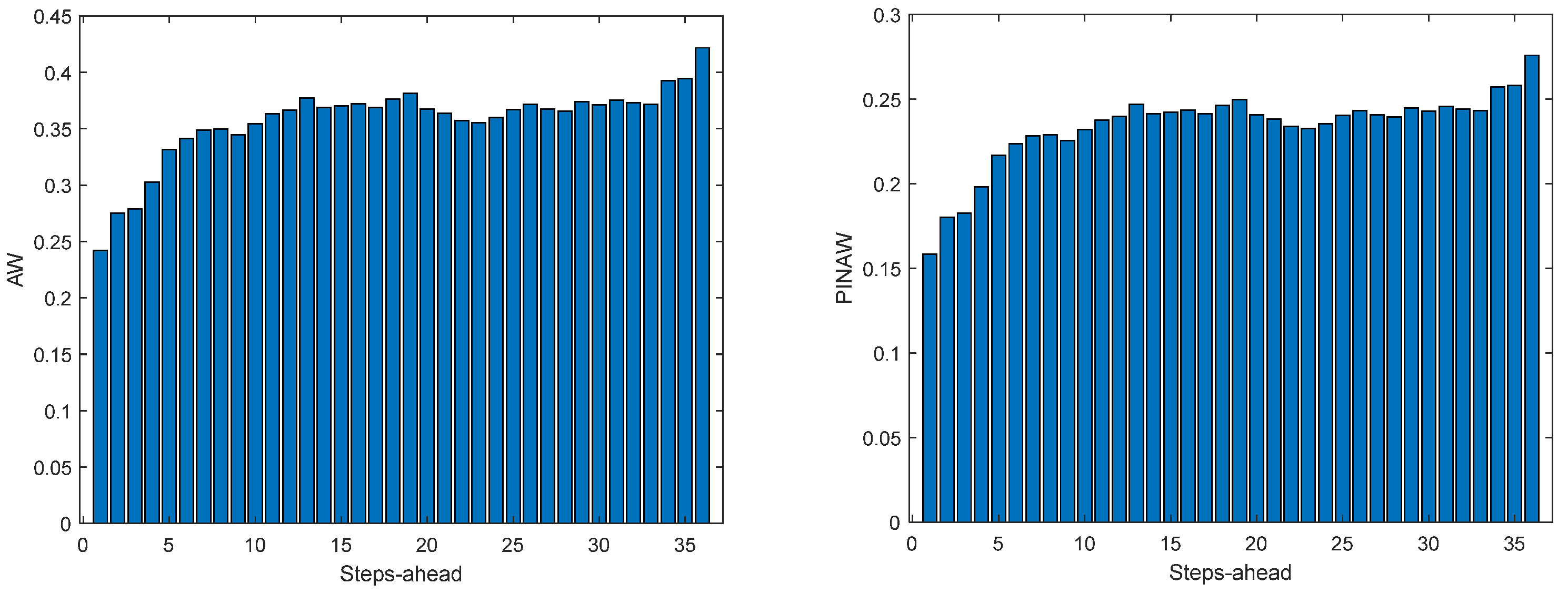
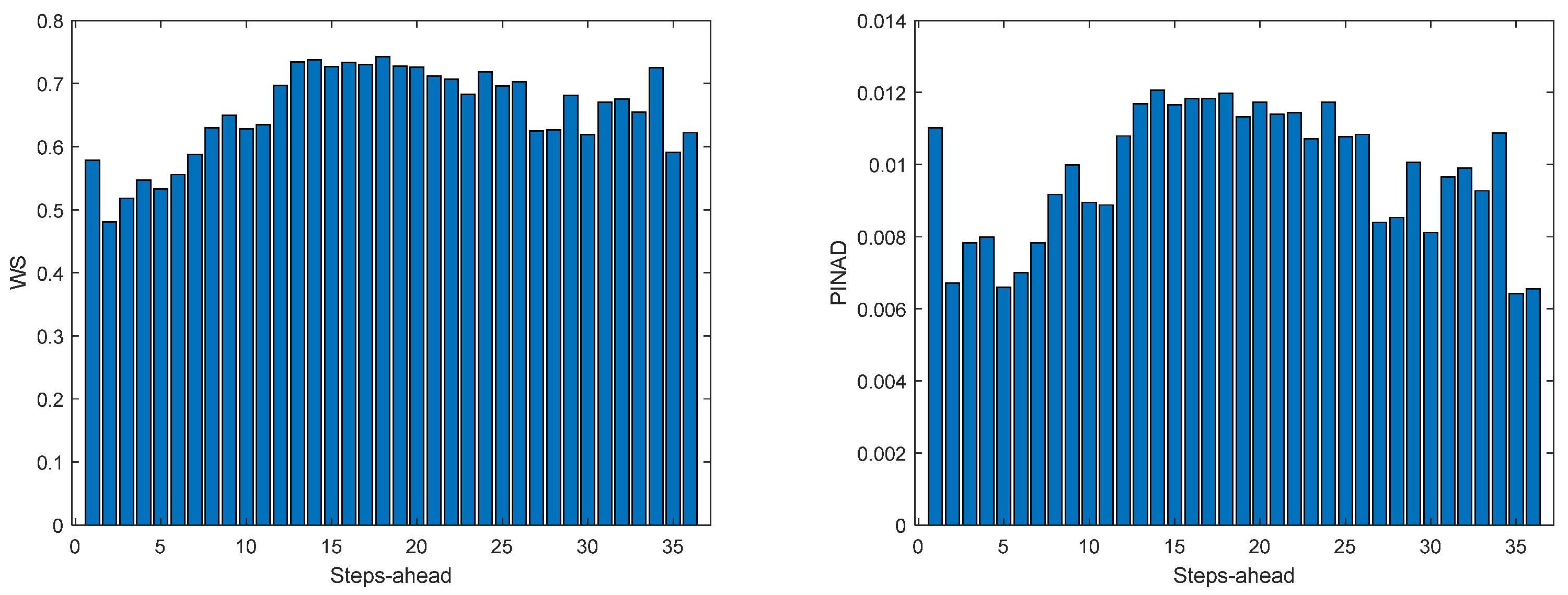
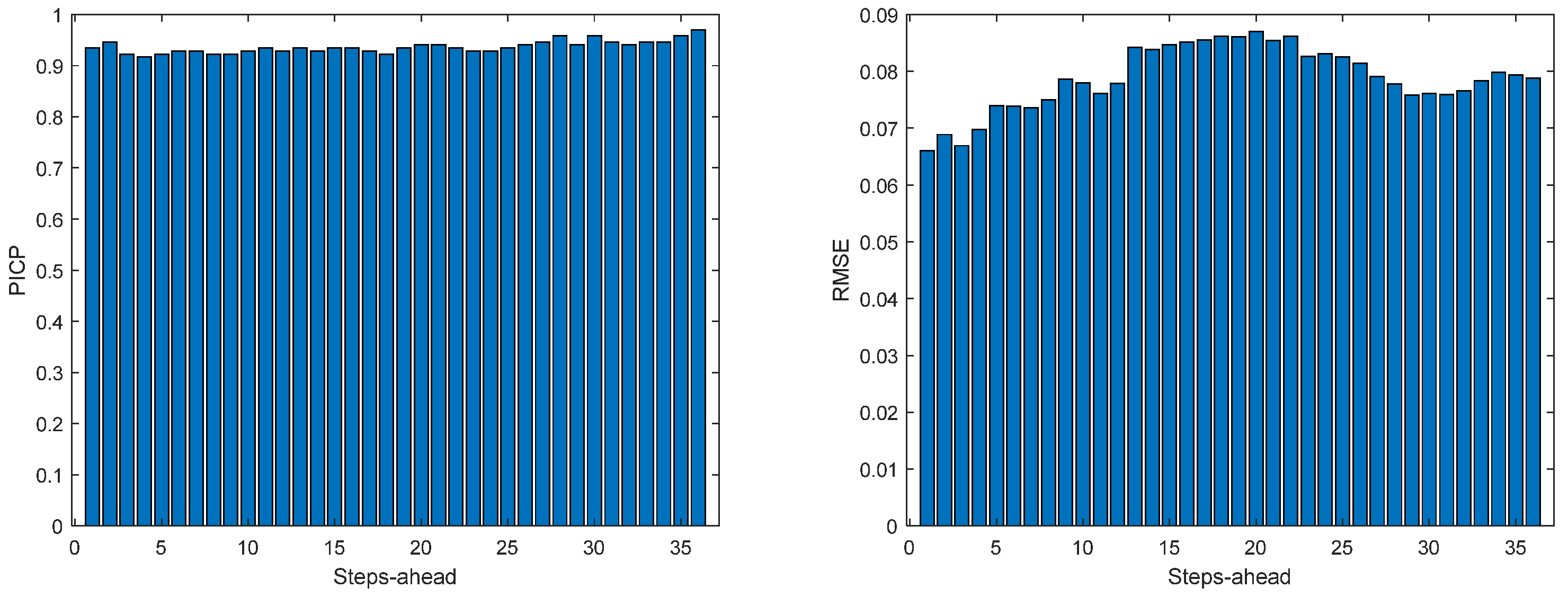
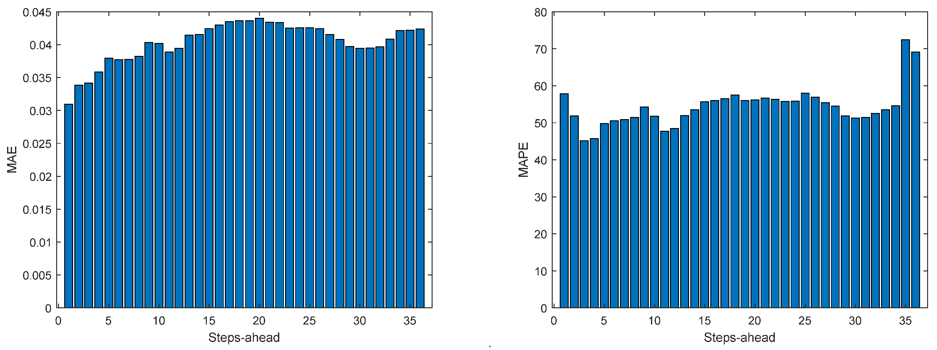
Air temperature is also a NAR model. Table 2 shows statistics corresponding to the mean of the employed performance criteria, averaged over the Prediction Horizon. The evolutions of the performance criteria are shown in Appendix A.1.
If Table 2 is compared with Table 1, as well as Figure 10, Figure 11, Figure 12, Figure 13 and Figure 14 with Figure A1, Figure A2, Figure A3, Figure A4 and Figure A5, it can be observed that every performance index, apart from PICP, is worse for the air temperature. One reason for this behavior might be that the solar radiation time series is much smoother than the atmospheric temperature or, in other words, the latter has more high-frequency content. This can be confirmed by examining Figure 19, which presents a snapshot of the air temperature snapshot.
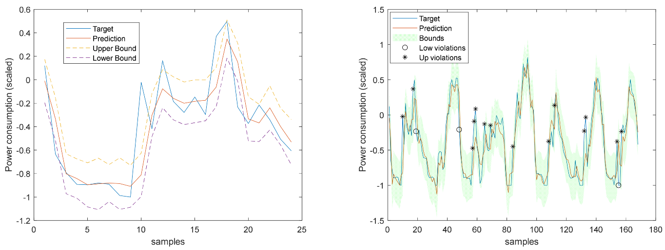
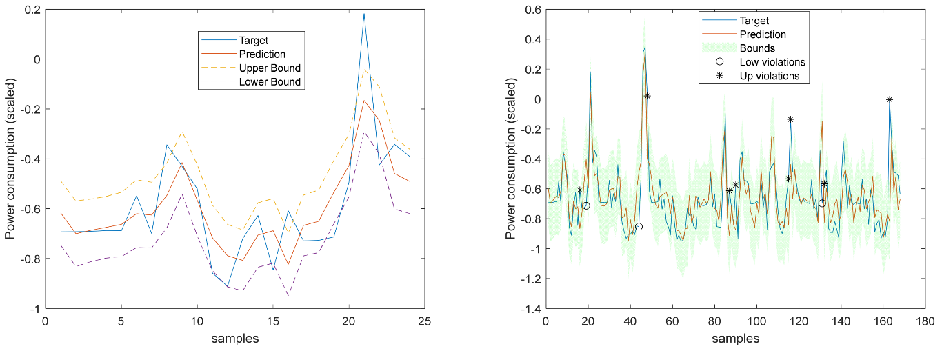
The blue line represents the time series, sampled at 1 s, and the red crosses the 1-h averages. It is clear that there is a substantial high-frequency content in the time series. 1SA forecasted signals are shown in Figure 20. Inspecting the right graph, only seven violations are present, corresponding to a PICP of 95%.
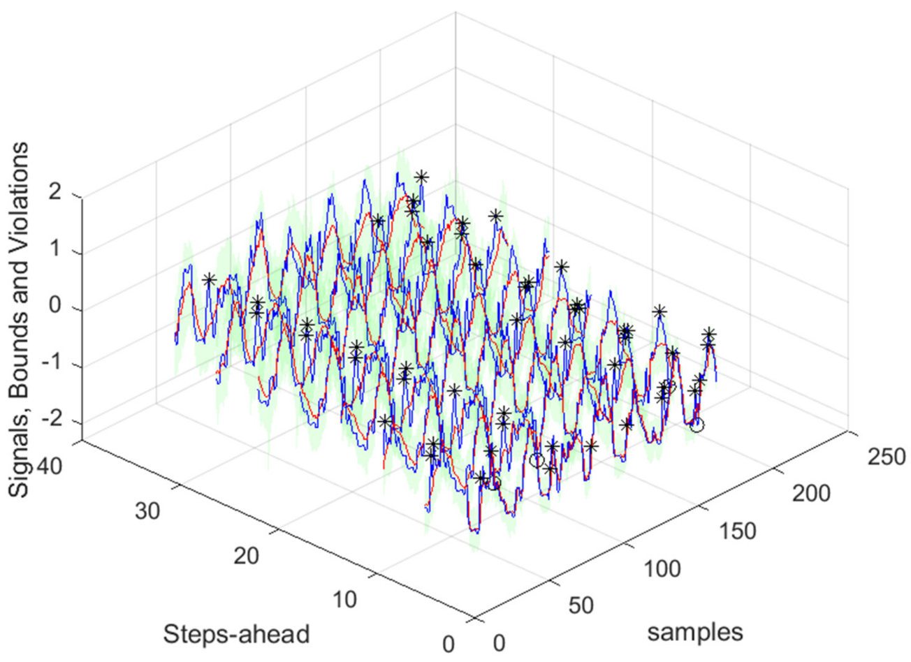
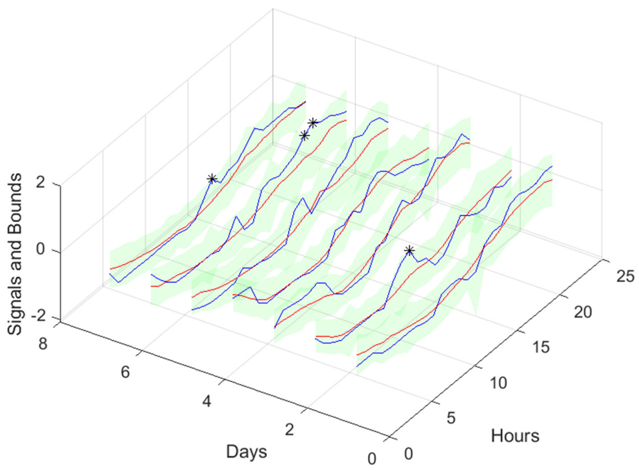
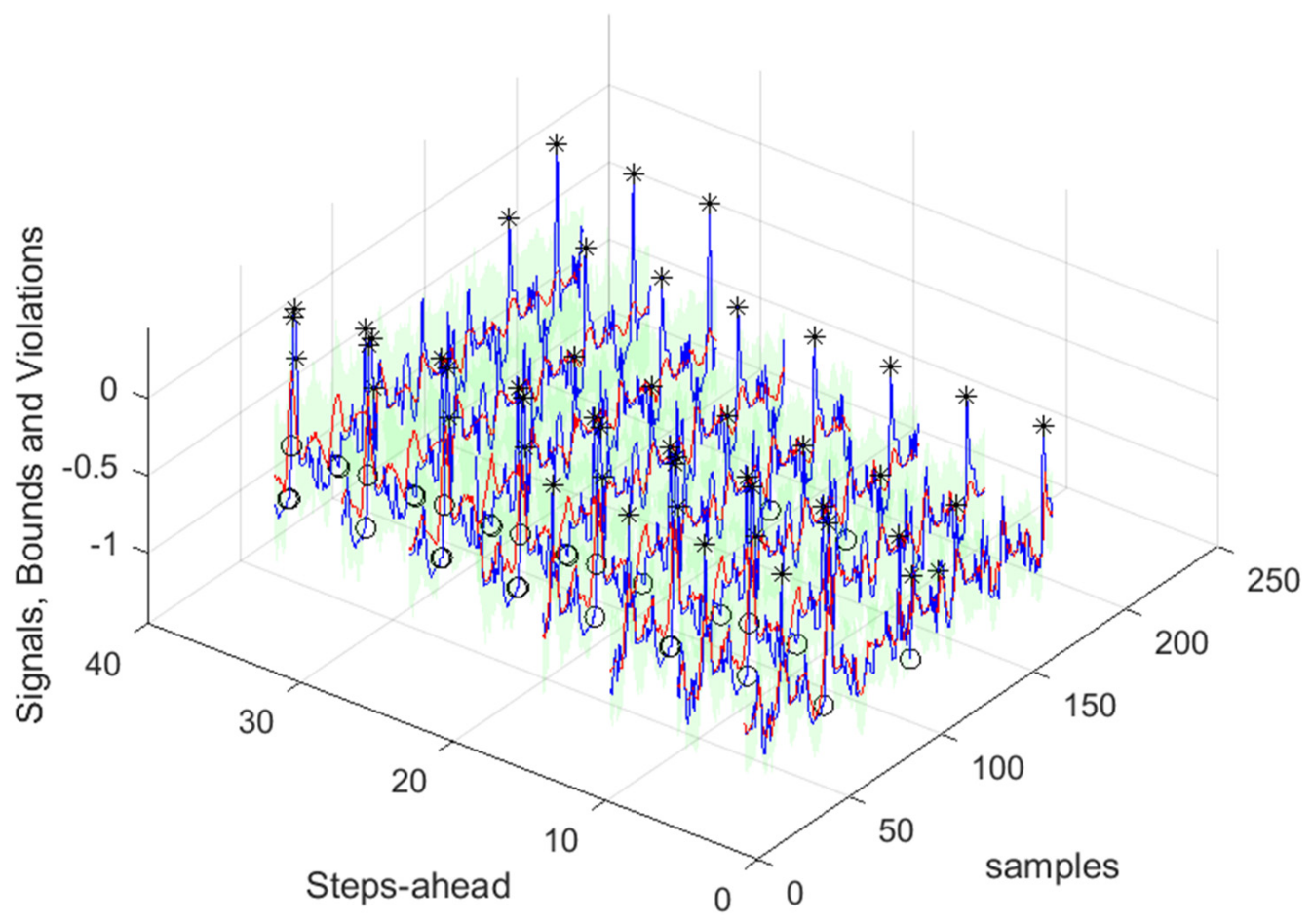
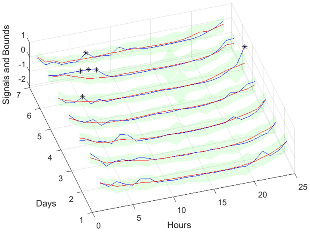
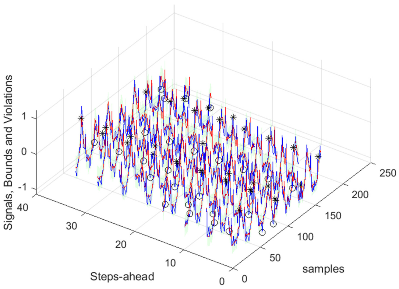
Looking at the number of violations for the steps ahead shown in Figure 21, the number of violations remains nearly constant with PH. Figure 22 shows the air temperature for the next day’s forecast.

3.4. Power Generation Models

Power Generation is a NARX model. Table 3 shows the same statistics, corresponding to the mean of the employed performance criteria, averaged over the Prediction Horizon. Relevant forecasts of the power generation are shown in Figure 23, Figure 24 and Figure 25. The evolutions of the performance criteria are shown in Appendix A.2.
The results of the power generation are similar (actually slightly better) to the solar radiation performance, as the most important exogenous variable for power generation is really the solar radiation.

3.5. Load Demand Models

These are NARX models. First, we shall address the load demand of each house individually. Then, using the four models, the load demand of the community using (47) will be evaluated. Finally, the community load demand with only one model, using (48), will be considered.

3.5.1. Monophasic House 1

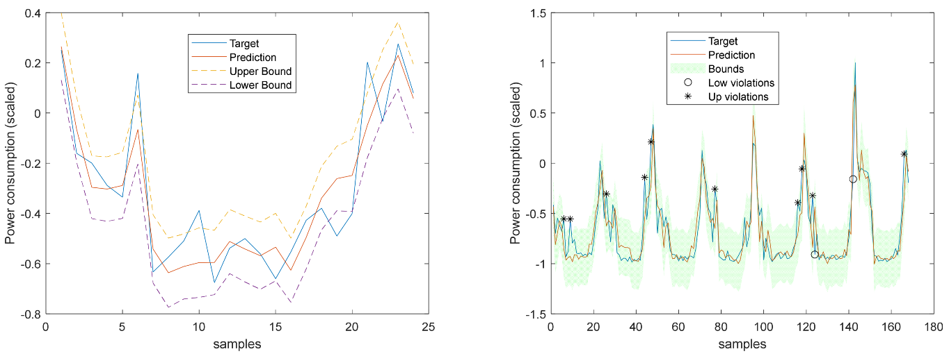
Table 4 shows the same statistics, corresponding to the mean of the employed performance criteria, averaged over the Prediction Horizon. Relevant forecasts of the load demand of monophasic House 1 are shown in Figure 26, Figure 27 and Figure 28. The evolutions of the performance criteria are shown in Appendix A.3.
The load demand for house 1 (and as it will be shown later, for all houses) obtains the worst results both in terms of fitting and robustness. To be able to maintain the PICP around (actually above) 0.9, the average width increases dramatically (please see Table 4 and figures in Appendix A.3). In contrast with the other variables analyzed before, the Winkler score is close to AW, which means that the penalties due to the width of the violations do not contribute significantly to WS.
The load demand time series of just one house is quite volatile, as the electric appliances are (a) not operated every day and (b) not used with the same schedule. For this reason, it is exceedingly difficult to obtain good forecasts.

3.5.2. Monophasic House 2

Table 5 shows the same statistics, corresponding to the mean of the employed performance criteria, averaged over the Prediction Horizon. Relevant forecasts of the load demand of monophasic House 2 are shown in Figure 29, Figure 30 and Figure 31. The evolutions of the performance criteria are shown in Appendix A.4.
Comparing the results of MP2 with MP1, the latter has a better performance. The average interval widths are smaller, although the average value of WS is similar, as it increases significantly along PH. The fitting is also better for MP2.

3.5.3. Triphasic House 1

Table 6 shows the same statistics, corresponding to the mean of the employed performance criteria, averaged over the Prediction Horizon. Relevant forecasts of the load demand of triphasic House 1 are shown in Figure 32, Figure 33 and Figure 34. The evolutions of the performance criteria are shown in Appendix A.5.
The same comments for the last case are applicable to TP1. It should be noticed, however, that the fitting ( R 2 ¯ ) is much worse.

3.5.4. Triphasic House 2

Table 7 shows the same statistics, corresponding to the mean of the employed performance criteria, averaged over the Prediction Horizon. Relevant forecasts of the load demand of triphasic House 2 are shown in Figure 35, Figure 36 and Figure 37. The evolutions of the performance criteria are shown in Appendix A.6.
The same comments for TP1 are applicable to TP2. It should also be noticed that the fitting ( R 2 ¯ ) of TP2 is much better.

3.5.5. Community Using (47)

Assume, without loss of generality, that our energy community has only two houses, whose loads are represented as Y ( 1 ) and Y ( 2 ) . We know that:
σ ε 2 1 + 2 = σ ε 2 1 + σ ε 2 2 + 2 C o v Y ( 1 ) , Y ( 2 )
where Cov denotes the covariance between two signals. As it has been found that the four loads are not cross-correlated, we shall assume:
σ ε 2 1 + 2 = σ ε 2 1 + σ ε 2 2
The standard error of the fit at y ^ k is given as:
φ ˘ k T x k , v ˘ Γ ˘ T Z ˘ t r , v ˘ Γ ˘ Z ˘ t r , v ˘ 1 φ ˘ k x k , v ˘
For the case of two houses:
Γ ˘ 1 + 2 Z ˘ t r , v ˘ 1 + 2 = Γ ˘ 1 Z ˘ t r 1 , v ˘ 1 Γ ˘ 2 Z ˘ t r 2 , v ˘ 2 ,
And using
φ ˘ k ( 1 + 2 ) x k , v ˘ 1 + 2 = φ ˘ k ( 1 ) x k , v ˘ 1 φ ˘ k ( 2 ) x k , v ˘ 2 ,
the standard error of the fit at y ^ k is given as:
φ ˘ k ( 1 ) x k , v ˘ 1 φ ˘ k ( 2 ) x k , v ˘ 2 T Γ ˘ 1 Z ˘ t r 1 , v ˘ 1 Γ ˘ 2 Z ˘ t r 2 , v ˘ 2 T Γ ˘ 1 Z ˘ t r 1 , v ˘ 1 Γ ˘ 2 Z ˘ t r 2 , v ˘ 2 1 φ ˘ k ( 1 ) x k , v ˘ 1 φ ˘ k ( 2 ) x k , v ˘ 2
Please note that in (54)–(56), the selected models for the houses change with each sample. To compute the bounds, (24) and (25) must be changed accordingly.
Table 8 shows the same statistics, corresponding to the mean of the employed performance criteria, averaged over the Prediction Horizon. Relevant forecasts of the community load demand are shown in Figure 38, Figure 39 and Figure 40. The evolutions of the performance criteria are shown in Appendix A.7.
Comparing Table 8 with Table 4, Table 5, Table 6 and Table 7 and the figures in Appendix A.7 with Appendix A.3, Appendix A.4, Appendix A.5 and Appendix A.6, we can observe that the performance obtained for the community load demand, using the sum of models, is similar to the ones achieved by each house individually.

3.5.6. Community Using (48)

Table 9 shows the same statistics, corresponding to the mean of the employed performance criteria, averaged over the Prediction Horizon. Relevant forecasts of the community load demand are shown in Figure 41, Figure 42 and Figure 43. The evolutions of the performance criteria are shown in Appendix A.8.
The results obtained with this approach are significantly better than those obtained using (47). Additionally, there is no need to design one ensemble model for each house in the community, which can be cumbersome if there are several households in the community. If we compare the values of Table 9 with Table 4, Table 5, Table 6 and Table 7, we can verify that in all indices, the community load demand is better for each house separately. The volatility of the time series reduces when the time series of several houses are combined, and, in principle, this volatility will reduce proportionally to the number of households in the community.

3.6. Net Load Demand Day-Ahead

Making use of the forecasts obtained for the community load demand, computed with (48), and for the power generated, we are able to forecast its difference, indicating the power that needs to be bought by the community (positive difference values) or sold by the community (negative values), together with the corresponding prediction bounds.
In the previous sections, scaled values were used to enable the performance values to be compared. Here, we need to use the original values.
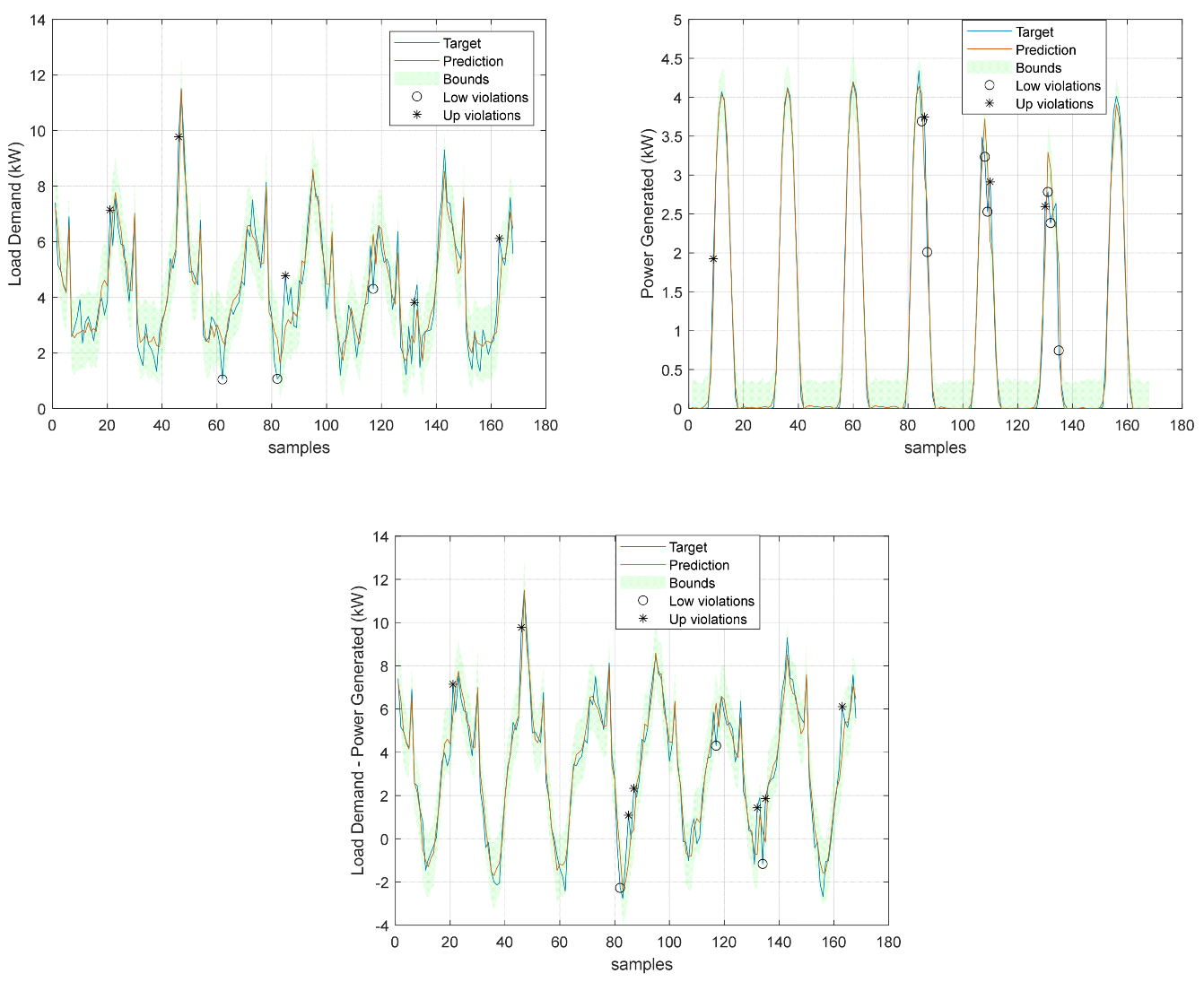
Figure 44 show these values for the prediction time series, where the lower bounds for both the load demand and power generated have been adjusted to ensure that power stays always positive.
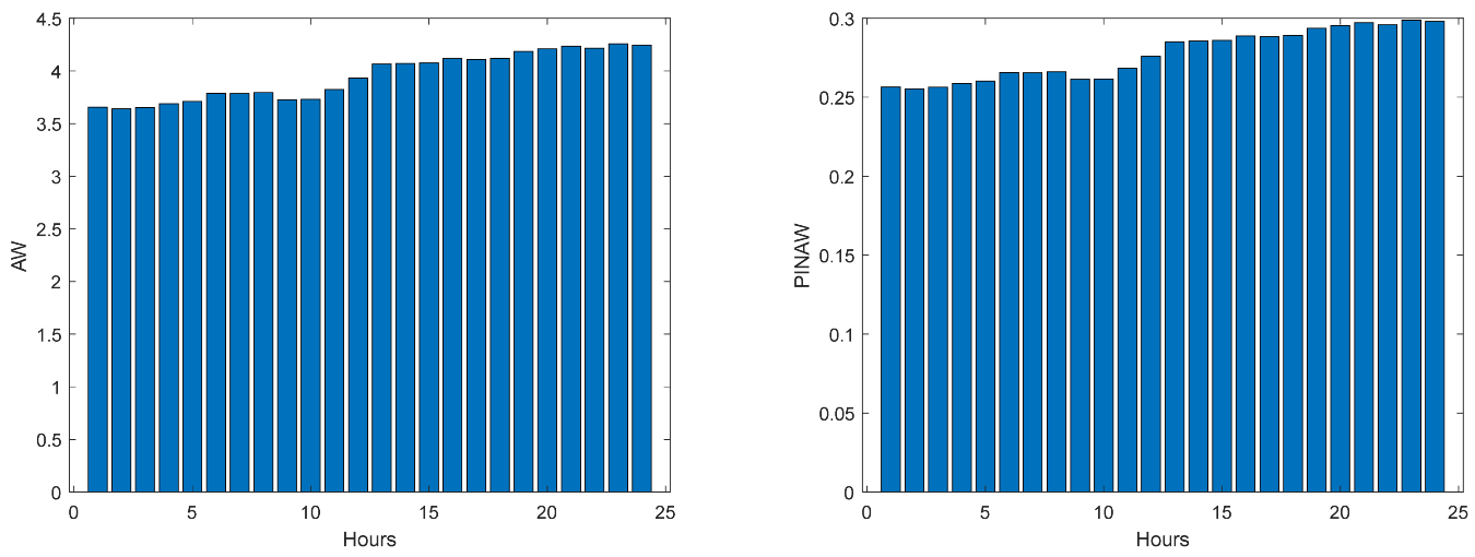
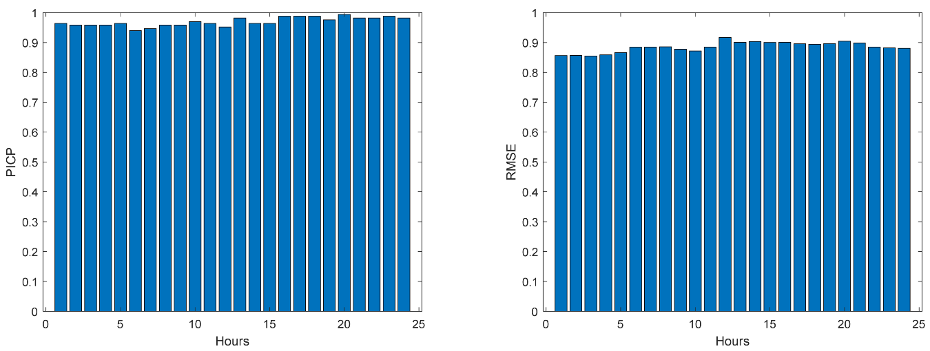
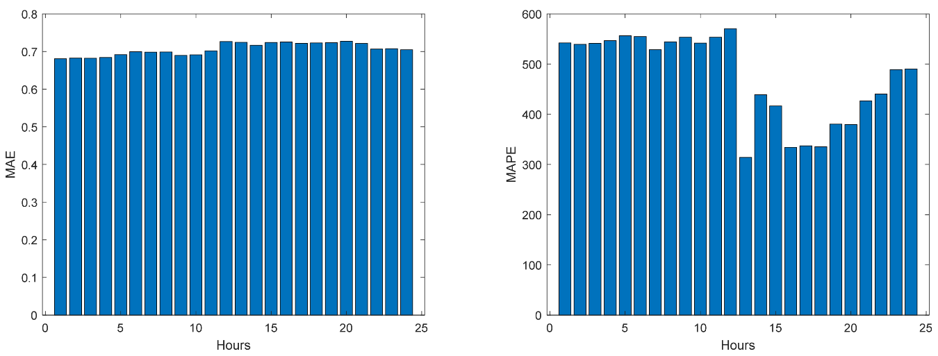
As we shall be interested in forecasts between 13 and 36 steps ahead (the next day values obtained at 12 o’clock the current day), the next results will only consider this range of steps ahead (Table 10).
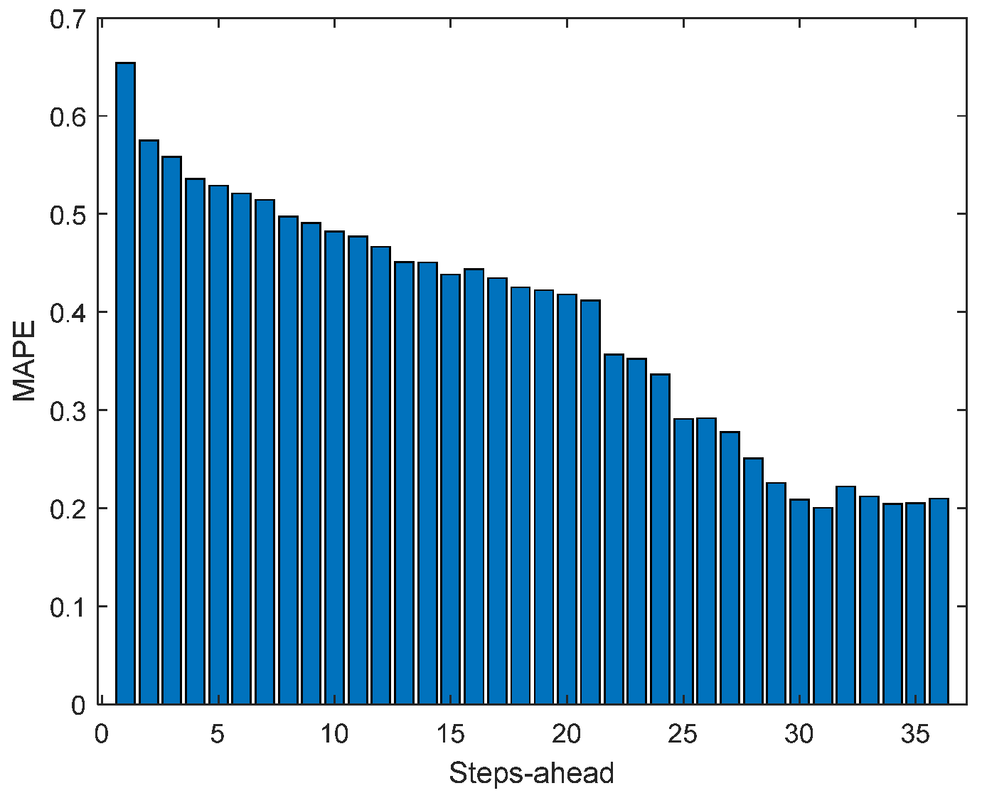
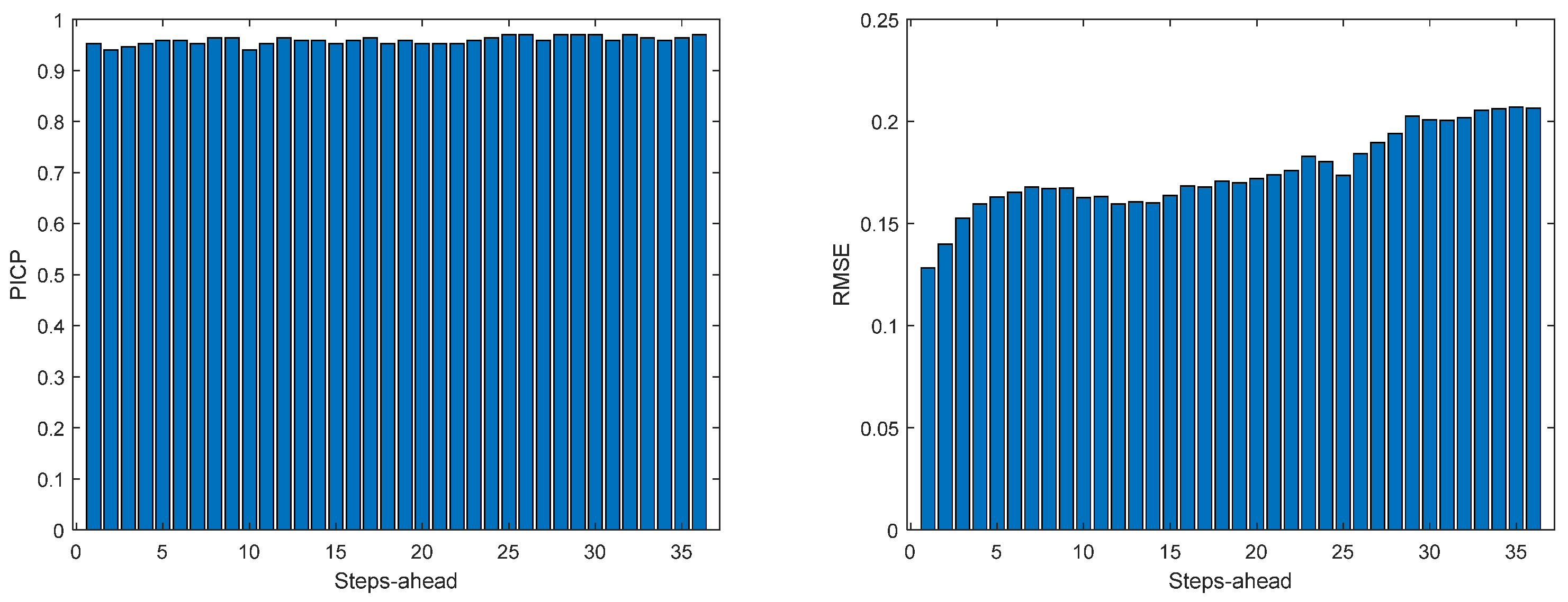
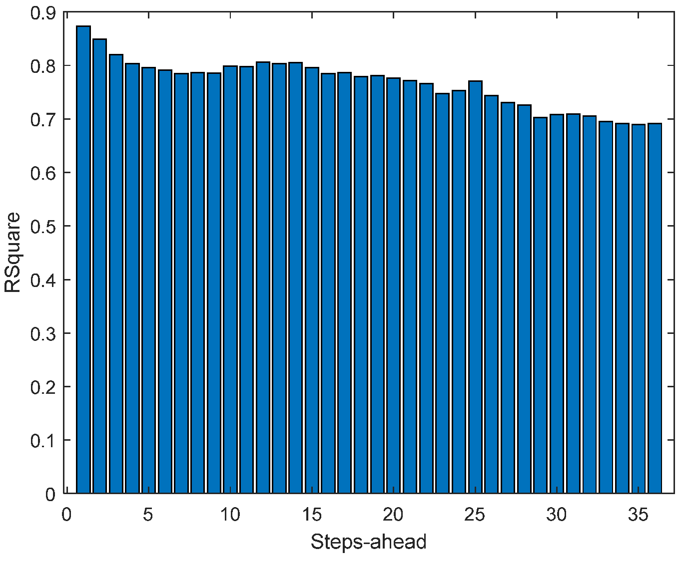
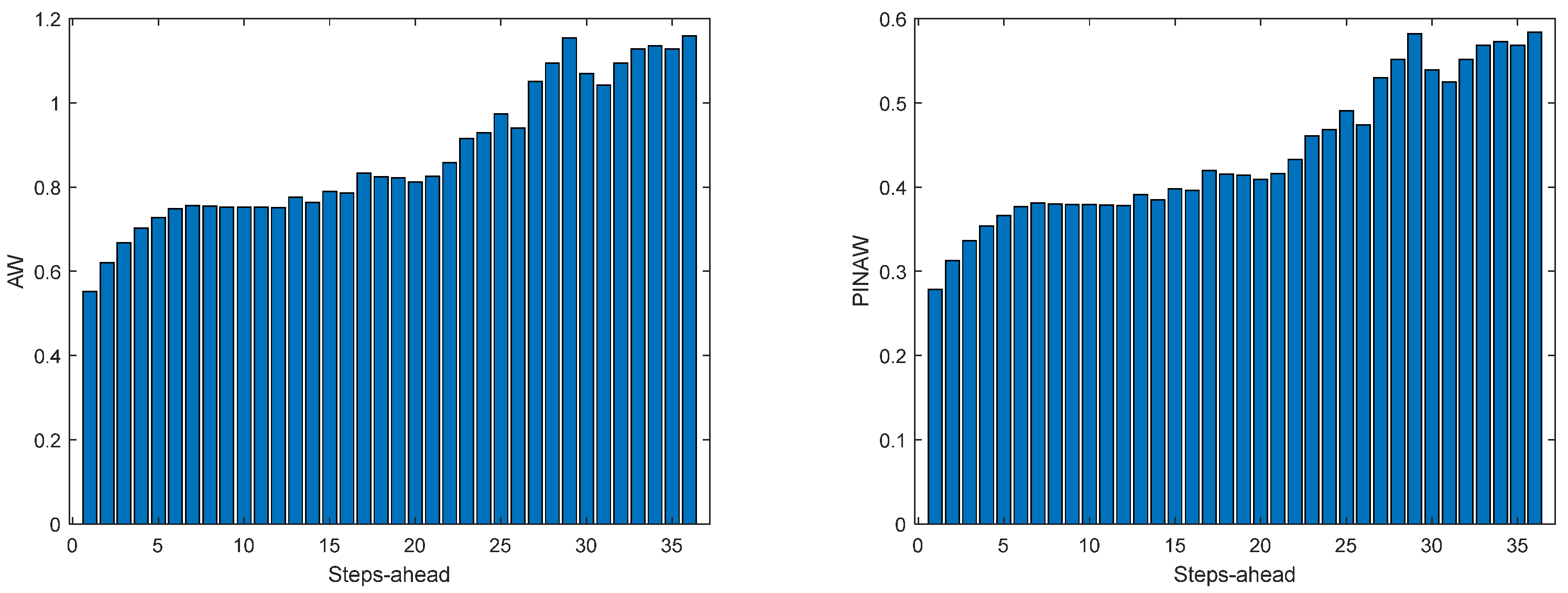
The evolutions of the performance criteria are shown in Figure 45, Figure 46, Figure 47, Figure 48 and Figure 49. Please notice that as the Net Load has a substantial number of values near 0, MAPE has very large values.
Relevant forecasts are shown in Figure 50 and Figure 51.
Please note that the number of upper (lower) violations is 35 (17) in a total of 1512 samples, which results in a PICP of 0.97.
There is one upper violation and two lower violations, resulting in a PICP of 0.98. As it can be seen, there is a particularly good fitting (R2 values above 0.9), and the P I N A W values are not so high, with an average value of 0.28, which is significantly smaller than the values obtained for the load demand of the individual houses. It is argued that for a larger energy community or for the union of different energy communities managed by the same aggregator, the results would be superior for the point forecast indices as well as the robustness indicators.

4. Discussion

Analyzing the results presented above, it can be concluded that the design procedure described in Section 2.2, together with the procedures described in Section 2.4 and Section 2.5, produce accurate models with a value of PICP almost constant throughout the prediction horizon. The average values presented in Table 1, Table 2, Table 3, Table 4, Table 5, Table 6, Table 7, Table 8, Table 9 and Table 10 are always higher than the desired confidence value of 0.9. For the evolution of the day-ahead net demand in the 7 days chosen, a PICP value of 0.98 is obtained, with an average PINAW value of 0.28. As there is a trade-off between PICP and AW, a smaller value of PINAW could be obtained by slightly decreasing PICP.
In what concerns the rest of the performance indices, in most cases, they increase with PH (except for R2, which decreases), as expected. But the increase (decrease) rate is not so high, which means that the forecasts are still useful for the day ahead. This behavior changes for the net load demand, as the performance indices are almost constant throughout the next day.
To assess the quality of the results, they should be compared with alternatives found in the literature. It is difficult to compare them quantitatively with rigor as, on the one hand, only one publication could be found for day-ahead net load demand, and, on the other hand, the contexts of the works in comparison are different between themselves and between this work. With those remarks in mind, we shall start with works that were briefly discussed in the introductory section on load demand and afterward on power generation.
Kychkin et al. [20] employ data from 4 houses located in Upper Austria, with data collected between 1 May 2016 to 31 August 2017. They compute at the end of one day the prediction for the next 24 h, with a 15 min sampling interval. Notice that in our case, we forecast the load demand for 36 h ahead, with a sampling interval of one hour. When the simulation period extends for several days, the models are retrained with data available until the end of each day. In our case, the models remain constant. For a simulation period of one week, which is equal to this paper, they obtained a normalized RMSE of 0.995 for the best single model and 0.96 for the best ensemble model. In our case, and using (48), a R M S E ¯ of 0.15 is obtained with scaled data. Assuming that the NRMSE is computed as (the paper does not clarify that):
N R M S E = R M S E y ¯
We obtain an NRMSE of 0.19. This value is smaller than the values obtained in the discussed paper even when, as pointed out, their model is retrained every day, and our forecasting horizon is larger.
Vilar and co-authors [9] employ probabilistic forecasting. As reported previously, they employed the whole Spanish load demand for the year 2012, not four houses as we did. They only employ the Average Width (AW) and the Winkler score as performance criteria. Using a confidence level of 95%, the yearly weekly average width is 5572 MW, and the Winkler Score is around 8872. The total demand value is omitted, but using Figure 1 of the paper, it should be around 20,000 MW. This way, the Prediction Interval Normalized Averaged Width (PINAW) should be around 28%, compared to 31% for our case. This way, similar PINAW are obtained for cases that are not comparable (4 households’ load demand against the whole Spanish load demand). In terms of WS, if we normalize the value shown in the paper by the total demand, a figure of 0.44 is obtained, which is the same value obtained in this paper.
Zhang and co-workers [12] use data from two cities and one region in China. The training set for Ottawa used data from 14 August 2019 to 28 August 2019 as a training set and from 29 August 2019 to 2 September 2019 for the test set. In the case of Baden-Württemberg, the training data was from 2 December 2019 to 16 December 2019, and the testing was set from 17 December 2019 to 21 December 2019. Finally, for the Chinese region, data from 11 December 2014 to 25 December 2014 were used for training, and data from 26 December 2014 to 30 December 2014 for testing. The best method (MCQRNNG) for the three sets of 5 days obtains MAPE values of 1.61, 1.74, and 1.47 for the cities of Ottawa, Baden-Württemberg, and the China region, respectively. In our case, a value of 0.87 is obtained for MAPE. Their measured PICP values were 0.88, 1, and 0.87. In our case, a value of 0.96 is obtained. Their PINAW values were 0.11, 0.14, and 0.08, while we obtained a higher value of 0.31. In the same way, as in the previous paper, we are comparing whole cities and regions with just four houses.
Addressing current PV generation forecasts, [26] used PV output power data acquired in a roof-mounted PV power generation system in China. The collected dataset includes a total of 364 days. The training set employed data from 1-300 days, the development set data from 301–332 days, and the test set data from days 333–364. The installation capacity is 2.8 MW. In our case, the capacity is only 6.9 kW. They used as performance indices the Normalized MAE, computed with (58), adapted to MAE, and the Winkler score, with a 90% confidence level. The average values computed for selected 6 days in the test set were 34.9% and 40.1. In our case, we obtain 24.9% and 1.9, respectively.
The work [22] uses data from 300 Australian houses. In each one of the houses, hourly load demand and PV generation values were recorded from 2010 to 2013. The dataset was partitioned into training (77%) and testing (23%). A prediction horizon of twenty-four steps is considered. Using the best model (Seq2Seq LSTM + GBRT), the average RMSE and MAE for the load demand were 4.53 and 3.39, respectively. The average load demand had to be estimated from Figure 10 of the paper, and it is roughly 35 kW. This is translated into normalized values of 0.13 and 0.11. Our figures are 0.19 and 0.15, with only four houses and a PH of 36 h. In terms of PV generation, the RMSE and MAE values are 2.5 and 1.19, respectively. Estimating the average value of 11 kW using Figure 11 of the paper, the normalized values obtained were 0.23 and 0.11. Our values are 0.25 and 0.13, which are similar.
Finally, as pointed out before, paper [27] is the only publication that has net load forecasting as its target. It uses meter data acquired, with a time interval resolution of 1 h, from a residential community with fifty-five houses in the IIT Bombay area. The only performance criterion that can be used is MAPE for load demand and PV generation. Assuming that the values shown in the paper are for the 24 h ahead and not for the one-step ahead, the MAPE values were 0.49 and 0.75 for one random day (15 May 2017). Our values are 0.87 and 0.54 for thirty-six forecasting steps for load demand and PV generation, respectively, for 7 days of testing. Therefore, the MAPE load demand for the fifty houses is better than ours for just four houses. In contrast, our results for PV generation are better than theirs.

5. Conclusions

We have proposed a simple method for producing both point estimates and prediction intervals for a one-day-ahead community net load demand. The prediction intervals obtained correspond to a very high confidence level (0.96) with a reasonable average Prediction Interval Normalized Averaged Width value of 0.28. As these values were obtained with a desired PICP value of 0.90, small PINAW values could be obtained by lowering the desired PICP value.
No direct comparison could be found in the literature. This way, comparisons were made indirectly by assessing the performance of load demand and PV generation forecasting alternatives. Regarding the former, for the only case with the same number of houses considered here, our proposal obtains much better point forecasting performance. All the other works employed a significantly large number of households, obtaining typically better results. As was demonstrated in the paper, there should be an improvement in results with an increase in the number of households. In relation to PV generation, our approach obtains similar or better results than the alternatives.
One point that should be stressed is that, in our approach, the forecasts are obtained by small, shallow artificial neural networks whose complexity is orders of magnitude smaller than the alternative models, which typically are deep models or ensembles of deep models. With the results obtained similar to or better than those of the competitors, it can be concluded that by employing parsimonious models designed with good data selection, feature selection, and parameter estimation algorithms, better results can be expected than by employing “brute force” deep models.
For all models described in this paper, the obtained PICP values were higher than the confidence level sought. This is obviously better than the opposite behavior, but in the future, we shall look at ways of obtaining PICP values more similar to the desired confidence level. Additionally, load demand model accuracy would be improved if estimations of controllable and monitored loads were available for the houses considered.

Author Contributions

The authors contributed equally to this work. Conceptualization, M.d.G.R. and A.R.; Software, A.R.; Validation, M.d.G.R.; Writing—original draft, M.d.G.R. and A.R.; Writing & editing, M.d.G.R. and A.R.; Funding acquisition, A.R. All authors have read and agreed to the published version of the manuscript.

Funding

The authors would like to acknowledge the support of Operational Program Portugal 2020 and Operational Program CRESC Algarve 2020, grant number 72581/2020. A.R. also acknowledges the support of Fundação para a Ciência e Tecnologia, grant UID/EMS/50022/2020, through IDMEC under LAETA. M.d.G.R. also acknowledges the support of the Foundation for Science and Technology, I.P./MCTES through national funds (PIDDAC), within the scope of CISUC R&D Unit—UIDB/00326/2020 or project code UIDP/00326/2020.

Data Availability Statement

Data employed in this work can be found in [41].

Conflicts of Interest

The authors declare no conflict of interest.

Appendix A

Appendix A.1. Atmospheric Air Temperature

Figure A1. Atmospheric Temperature AW (left) and PINAW (right) forecasts.
Energies 17 00696 g0a1
Figure A2. Atmospheric Temperature WS (left) and PINAD (right) forecasts.
Energies 17 00696 g0a2
Figure A3. Atmospheric Temperature PICP (left) and RMSE (right) forecasts.
Energies 17 00696 g0a3
Figure A4. Atmospheric Temperature MAE (left) and MAPE (right) forecasts.
Energies 17 00696 g0a4
Figure A5. Atmospheric Temperature R2 forecast.
Energies 17 00696 g0a5

Appendix A.2. Power Generation

Figure A6. Power Generation AW (left) and PINAW (right) forecasts.
Energies 17 00696 g0a6
Figure A7. Power Generation WS (left) and PINAD (right) forecasts.
Energies 17 00696 g0a7
Figure A8. Power Generation PICP (left) and RMSE (right) forecasts.
Energies 17 00696 g0a8
Figure A9. Power Generation MAE (left) and MAPE (right) forecasts.
Energies 17 00696 g0a9
Figure A10. Power Generation R2 forecast.
Energies 17 00696 g0a10

Appendix A.3. Monophasic House 1

Figure A11. MP1 Load Demand AW (left) and PINAW (right) evolutions.
Energies 17 00696 g0a11
Figure A12. MP1 Load Demand WS (left) and PINAD (right) evolutions.
Energies 17 00696 g0a12
Figure A13. MP1 Load Demand PICP (left) and RMSE (right) evolutions.
Energies 17 00696 g0a13
Figure A14. MP1 Load Demand MAE (left) and MAPE (right) evolutions.
Energies 17 00696 g0a14
Figure A15. MP1 Load Demand R2 evolution.
Energies 17 00696 g0a15

Appendix A.4. Monophasic House 2

Figure A16. MP2 Load Demand AW (left) and PINAW (right) evolutions.
Energies 17 00696 g0a16
Figure A17. MP2 Load Demand WS (left) and PINAD (right) evolutions.
Energies 17 00696 g0a17
Figure A18. MP2 Load Demand PICP (left) and RMSE (right) evolutions.
Energies 17 00696 g0a18
Figure A19. MP2 Load Demand MAE (left) and MAPE (right) evolutions.
Energies 17 00696 g0a19
Figure A20. MP2 Load Demand R2 evolution.
Energies 17 00696 g0a20

Appendix A.5. Triphasic House 1

Figure A21. TP1 Load Demand AW (left) and PINAW (right) evolutions.
Energies 17 00696 g0a21
Figure A22. TP1 Load Demand WS (left) and PINAD (right) evolutions.
Energies 17 00696 g0a22
Figure A23. TP1 Load Demand PICP (left) and RMSE (right) evolutions.
Energies 17 00696 g0a23
Figure A24. TP1 Load Demand MAE (left) and MAPE (right) evolutions.
Energies 17 00696 g0a24
Figure A25. TP1 R2 evolution.
Energies 17 00696 g0a25

Appendix A.6. Triphasic House 2

Figure A26. TP2 Load Demand AW (left) and PINAW (right) evolutions.
Energies 17 00696 g0a26
Figure A27. TP2 Load Demand WS (left) and PINAD (right) evolutions.
Energies 17 00696 g0a27
Figure A28. TP2 Load Demand PICP (left) and RMSE (right) evolutions.
Energies 17 00696 g0a28
Figure A29. TP2 Load Demand MAE (left) and MAPE (right) evolutions.
Energies 17 00696 g0a29
Figure A30. TP2 Load Demand R2 evolution.
Energies 17 00696 g0a30

Appendix A.7. Community Using (41)

Figure A31. Community Load Demand AW (left) and PINAW (right) evolutions.
Energies 17 00696 g0a31
Figure A32. Community Load Demand WS (left) and PINAD (right) evolutions.
Energies 17 00696 g0a32
Figure A33. Community Load Demand PICP (left) and RMSE (right) evolutions.
Energies 17 00696 g0a33
Figure A34. Community Load Demand MAE (left) and MAPE (right) evolutions.
Energies 17 00696 g0a34
Figure A35. Community Load Demand R2 evolution.
Energies 17 00696 g0a35

Appendix A.8. Community Using (42)

Figure A36. Community Load Demand AW (left) and PINAW (right) evolutions.
Energies 17 00696 g0a36
Figure A37. Community Load Demand WS (left) and PINAD (right) evolutions.
Energies 17 00696 g0a37
Figure A38. Community Load Demand PICP (left) and RMSE (right) evolutions.
Energies 17 00696 g0a38
Figure A39. Community Load Demand MAE (left) and MAPE (right) evolutions.
Energies 17 00696 g0a39
Figure A40. Community Load Demand R2 evolution.
Energies 17 00696 g0a40

References

  1. Gomes, I.L.R.; Ruano, M.G.; Ruano, A.E. From home energy management systems to communities energy managers: The use of an intelligent aggregator in a community in Algarve, Portugal. Energy Build. 2023, 298, 113588. [Google Scholar] [CrossRef]
  2. Yang, L.; Li, X.; Sun, M.; Sun, C. Hybrid Policy-Based Reinforcement Learning of Adaptive Energy Management for the Energy Transmission-Constrained Island Group. IEEE Trans. Ind. Inform. 2023, 19, 10751–10762. [Google Scholar] [CrossRef]
  3. Carriere, T.; Kariniotakis, G. An Integrated Approach for Value-Oriented Energy Forecasting and Data-Driven Decision-Making Application to Renewable Energy Trading. IEEE Trans. Smart Grid 2019, 10, 6933–6944. [Google Scholar] [CrossRef]
  4. Schreck, S.; Comble, I.P.d.L.; Thiem, S.; Niessen, S. A Methodological Framework to support Load Forecast Error Assessment in Local Energy Markets. IEEE Trans. Smart Grid 2020, 11, 3212–3220. [Google Scholar] [CrossRef]
  5. Suganthi, L.; Samuel, A.A. Energy models for demand forecasting—A review. Renew. Sustain. Energy Rev. 2012, 16, 1223–1240. [Google Scholar] [CrossRef]
  6. Hong, T.; Fan, S. Probabilistic electric load forecasting: A tutorial review. Int. J. Forecast. 2016, 32, 914–938. [Google Scholar] [CrossRef]
  7. Weron, R. Electricity price forecasting: A review of the state-of-the-art with a look into the future. Int. J. Forecast. 2014, 30, 1030–1081. [Google Scholar] [CrossRef]
  8. Nowotarski, J.; Weron, R. Recent advances in electricity price forecasting: A review of probabilistic forecasting. Renew. Sustain. Energy Rev. 2018, 81, 1548–1568. [Google Scholar] [CrossRef]
  9. Vilar, J.; Aneiros, G.; Raña, P. Prediction intervals for electricity demand and price using functional data. Int. J. Electr. Power Energy Syst. 2018, 96, 457–472. [Google Scholar] [CrossRef]
  10. Grothe, O.; Kächele, F.; Krüger, F. From point forecasts to multivariate probabilistic forecasts: The Schaake shuffle for day-ahead electricity price forecasting. Energy Econ. 2023, 120, 106602. [Google Scholar] [CrossRef]
  11. Ferreira, P.M.; Cuambe, I.D.; Ruano, A.E.; Pestana, R. Forecasting the Portuguese Electricity Consumption using Least-Squares Support Vector Machines. In Proceedings of the 3rd IFAC Conference on Intelligent Control and Automation Science ICONS 2013, Chengdu, China, 2–4 September 2013; Volume 46, pp. 411–416. [Google Scholar] [CrossRef]
  12. Zhang, W.; He, Y.; Yang, S. Day-ahead load probability density forecasting using monotone composite quantile regression neural network and kernel density estimation. Electr. Power Syst. Res. 2021, 201, 107551. [Google Scholar] [CrossRef]
  13. Bracale, A.; Caramia, P.; De Falco, P.; Hong, T. A Multivariate Approach to Probabilistic Industrial Load Forecasting. Electr. Power Syst. Res. 2020, 187, 106430. [Google Scholar] [CrossRef]
  14. Cartagena, O.; Parra, S.; Muñoz-Carpintero, D.; Marín, L.G.; Sáez, D. Review on Fuzzy and Neural Prediction Interval Modelling for Nonlinear Dynamical Systems. IEEE Access 2021, 9, 23357–23384. [Google Scholar] [CrossRef]
  15. Ungar, L.; De, R.; Rosengarten, V. Estimating Prediction Intervals for Artificial Neural Networks. In Proceedings of the 9th Yale Workshop on Adaptive and Learning Systems, New Haven, CT, USA, 10 May 1996; pp. 1–6. [Google Scholar]
  16. Hwang, J.T.G.; Ding, A.A. Prediction Intervals for Artificial Neural Networks. J. Am. Stat. Assoc. 1997, 92, 748–757. [Google Scholar] [CrossRef]
  17. Beyaztas, U.; Shang, H.L. Robust bootstrap prediction intervals for univariate and multivariate autoregressive time series models. J. Appl. Stat. 2022, 49, 1179–1202. [Google Scholar] [CrossRef]
  18. Nix, D.A.; Weigend, A.S. Estimating the mean and variance of the target probability distribution. In Proceedings of the 1994 IEEE International Conference on Neural Networks (ICNN’94), Orlando, FL, USA, 28 June–2 July 1994; Volume 51, pp. 55–60. [Google Scholar]
  19. Škrjanc, I. Fuzzy confidence interval for pH titration curve. Appl. Math. Model. 2011, 35, 4083–4090. [Google Scholar] [CrossRef]
  20. Kychkin, A.V.; Chasparis, G.C. Feature and model selection for day-ahead electricity-load forecasting in residential buildings. Energy Build. 2021, 249, 111200. [Google Scholar] [CrossRef]
  21. Kiprijanovska, I.; Stankoski, S.; Ilievski, I.; Jovanovski, S.; Gams, M.; Gjoreski, H. HousEEC: Day-Ahead Household Electrical Energy Consumption Forecasting Using Deep Learning. Energies 2020, 13, 2672. [Google Scholar] [CrossRef]
  22. Pirbazari, A.M.; Sharma, E.; Chakravorty, A.; Elmenreich, W.; Rong, C. An Ensemble Approach for Multi-Step Ahead Energy Forecasting of Household Communities. IEEE Access 2021, 9, 36218–36240. [Google Scholar] [CrossRef]
  23. Pecan Street Inc. Dataport. Available online: https://www.pecanstreet.org/dataport/ (accessed on 1 January 2024).
  24. Yang, T.; Li, B.; Xun, Q. LSTM-Attention-Embedding Model-Based Day-Ahead Prediction of Photovoltaic Power Output Using Bayesian Optimization. IEEE Access 2019, 7, 171471–171484. [Google Scholar] [CrossRef]
  25. Fonseca, J.G.D.; Ohtake, H.; Oozeki, T.; Ogimoto, K. Prediction Intervals for Day-Ahead Photovoltaic Power Forecasts with Non-Parametric and Parametric Distributions. J. Electr. Eng. Technol. 2018, 13, 1504–1514. [Google Scholar] [CrossRef]
  26. Mei, F.; Gu, J.; Lu, J.; Lu, J.; Zhang, J.; Jiang, Y.; Shi, T.; Zheng, J. Day-Ahead Nonparametric Probabilistic Forecasting of Photovoltaic Power Generation Based on the LSTM-QRA Ensemble Model. IEEE Access 2020, 8, 166138–166149. [Google Scholar] [CrossRef]
  27. Saini, V.K.; Al-Sumaiti, A.S.; Kumar, R. Data driven net load uncertainty quantification for cloud energy storage management in residential microgrid. Electr. Power Syst. Res. 2024, 226, 109920. [Google Scholar] [CrossRef]
  28. Ruano, A.; Ruano, M.d.G. Designing Robust Forecasting Ensembles of Data-Driven Models with a Multi-Objective Formulation: An Application to Home Energy Management Systems. Inventions 2023, 8, 96. [Google Scholar] [CrossRef]
  29. Khosravani, H.R.; Ruano, A.E.; Ferreira, P.M. A convex hull-based data selection method for data driven models. Appl. Soft Comput. 2016, 47, 515–533. [Google Scholar] [CrossRef]
  30. Ferreira, P.; Ruano, A. Evolutionary Multiobjective Neural Network Models Identification: Evolving Task-Optimised Models. In New Advances in Intelligent Signal Processing; Ruano, A., Várkonyi-Kóczy, A., Eds.; Studies in Computational Intelligence; Springer: Berlin/Heidelberg, Germany, 2011; Volume 372, pp. 21–53. [Google Scholar]
  31. Ruano, A.E.; Ferreira, P.M.; Cabrita, C.; Matos, S. Training Neural Networks and Neuro-Fuzzy Systems: A Unified View. IFAC Proc. Vol. 2002, 35, 415–420. [Google Scholar] [CrossRef]
  32. Ruano, A.E.B.; Jones, D.I.; Fleming, P.J. A New Formulation of the Learning Problem for a Neural Network Controller. In Proceedings of the 30th IEEE Conference on Decision and Control, Brighton, UK, 11–13 December 1991; pp. 865–866. [Google Scholar]
  33. Levenberg, M. A method for the solution of certain non-linear problems in least squares. Q. Appl. Math. 1964, 2, 164–168. [Google Scholar] [CrossRef]
  34. Marquardt, D.W. An Algorithm for Least-Squares Estimation of Nonlinear Parameters. J. Soc. Ind. Appl. Math. 1963, 11, 431–441. [Google Scholar] [CrossRef]
  35. Haykin, S. Neural Networks: A Comprehensive Foundation, 2nd ed.; Prentice Hall: Hoboken, NJ, USA, 1999. [Google Scholar]
  36. van der Meer, D.W.; Widen, J.; Munkhammar, J. Review on probabilistic forecasting of photovoltaic power production and electricity consumption. Renew. Sust. Energ. Rev. 2018, 81, 1484–1512. [Google Scholar] [CrossRef]
  37. Kath, C.; Ziel, F. Conformal prediction interval estimation and applications to day-ahead and intraday power markets. Int. J. Forecast. 2021, 37, 777–799. [Google Scholar] [CrossRef]
  38. Winkler, R.L. A Decision-Theoretic Approach to Interval Estimation. J. Am. Stat. Assoc. 1972, 67, 187–191. [Google Scholar] [CrossRef]
  39. Ruano, A.; Bot, K.; Ruano, M.G. Home Energy Management System in an Algarve residence. First results. In Proceedings of the 14th APCA International Conference on Automatic Control and Soft Computing, CONTROLO 2020, Bragança, Portugal, 1–3 June 2020; José, G., Manuel, B.-C., João Paulo, C., Eds.; Lecture Notes in Electrical Engineering; Springer Science and Business Media Deutschland GmbH: Bragança, Portugal, 2021; Volume 695, pp. 332–341. [Google Scholar]
  40. Gomes, I.L.R.; Ruano, M.G.; Ruano, A.E. MILP-based model predictive control for home energy management systems: A real case study in Algarve, Portugal. Energy Build. 2023, 281, 112774. [Google Scholar] [CrossRef]
  41. Ruano, A.; Ruano, M.G. HEMStoEC: Home Energy Management Systems to Energy Communities DataSet; Zenodo: Genève, Switzerland, 2023. [Google Scholar] [CrossRef]
  42. Ferreira, P.M.; Ruano, A.E.; Pestana, R.; Koczy, L.T. Evolving RBF predictive models to forecast the Portuguese electricity consumption. In Proceedings of the 2nd IFAC Conference on Intelligent Control Systems and Signal Processing, ICONS 2009, Istanbul, Turkey, 21–23 September 2009; Volume 42, pp. 414–419. [Google Scholar] [CrossRef]
  43. Chinrunngrueng, C.; Séquin, C.H. Optimal adaptive k-means algorithm with dynamic adjustment of learning rate. IEEE Trans. Neural Netw. 1995, 6, 157–169. [Google Scholar] [CrossRef] [PubMed]
Figure 1. Model design fluxogram.
Energies 17 00696 g001
Figure 2. Solar Radiation. Left: 1st period; Right: 2nd period.
Energies 17 00696 g002
Figure 3. Atmospheric Temperature. Left: 1st period; Right: 2nd period.
Energies 17 00696 g003
Figure 4. Day Code. Left: 1st period; Right: 2nd period.
Energies 17 00696 g004
Figure 5. Power Demand: House 1 (monophasic). Left: 1st period; Right: 2nd period.
Energies 17 00696 g005
Figure 6. Power Demand: House 2 (monophasic). Left: 1st period; Right: 2nd period.
Energies 17 00696 g006
Figure 7. Power Demand: House 3 (triphasic). Left: 1st period; Right: 2nd period.
Energies 17 00696 g007
Figure 8. Power Demand: House 4 (triphasic). Left: 1st period; Right: 2nd period.
Energies 17 00696 g008
Figure 9. Community Power Generated. Left: 1st period; Right: 2nd period.
Energies 17 00696 g009
Figure 10. Power delays and forecasts.
Energies 17 00696 g010
Figure 11. Solar Radiation AW (left) and PINAW (right) forecasts.
Energies 17 00696 g011
Figure 12. Solar Radiation WS (left) and PINAD (right) forecasts.
Energies 17 00696 g012
Figure 13. Solar Radiation PICP (left) and RMSE (right) forecasts.
Energies 17 00696 g013
Figure 14. Solar Radiation MAE (left) and MAPE (right) forecasts.
Energies 17 00696 g014
Figure 15. Solar Radiation R2 forecasts.
Energies 17 00696 g015
Figure 16. Solar Radiation 1-step-ahead. Left: One Day; Right: All days in the prediction time series. The ‘o’ symbols denote the target upper bound violations, and the symbols ‘*’ are the lower bound violations by the target. The x-axis label denotes the samples of the prediction time series.
Energies 17 00696 g016
Figure 17. Solar Radiation [1, 5, 11, …, 36]-steps-ahead. The same notation of Figure 16 right is used.
Energies 17 00696 g017
Figure 18. Solar Radiation next-day forecast is computed with data measured up to 12 h the day before. The same notation of Figure 15 right is used.
Energies 17 00696 g018
Figure 19. Air temperature snapshot.
Energies 17 00696 g019
Figure 20. Atmospheric Temperature 1-step-ahead. Left: One Day; Right: All days in the prediction time series.
Energies 17 00696 g020
Figure 21. Atmospheric Temperature [1, 5, 11, …, 36]-steps-ahead.
Energies 17 00696 g021
Figure 22. Atmospheric Temperature next-day forecast, with measured data until 12 h the day before.
Energies 17 00696 g022
Figure 23. Power Generation 1-step-ahead. Left: One Day; Right: All days in the prediction time series.
Energies 17 00696 g023
Figure 24. Power Generation [1, 5, 11, …, 36]-steps-ahead.
Energies 17 00696 g024
Figure 25. Power Generation next-day forecast, with measured data until 12 h the day before.
Energies 17 00696 g025
Figure 26. MP1 Load Demand 1-step-ahead. Left: One Day; Right: All days in the prediction time series.
Energies 17 00696 g026
Figure 27. MP1 Load Demand [1, 5, 11, …, 36]-steps-ahead.
Energies 17 00696 g027
Figure 28. MP1 Load Demand next-day forecast, with measured data until 12 h the day before.
Energies 17 00696 g028
Figure 29. MP2 Load Demand 1-step-ahead. Left: One Day; Right: All days in the prediction time series.
Energies 17 00696 g029
Figure 30. MP2 Load Demand [1, 5, 11, …, 36]-steps-ahead.
Energies 17 00696 g030
Figure 31. MP2 Load Demand next-day forecast, with measured data until 12 h the day before.
Energies 17 00696 g031
Figure 32. TP1 Load Demand 1-step-ahead. Left: One Day; Right: All days in the prediction time series.
Energies 17 00696 g032
Figure 33. TP1 Load Demand [1, 5, 11, …, 36]-steps-ahead.
Energies 17 00696 g033
Figure 34. TP1 Load Demand next-day forecast, with measured data until 12 h the day before.
Energies 17 00696 g034
Figure 35. TP2 Load Demand 1-step-ahead. Left: One Day; Right: All days in the prediction time series.
Energies 17 00696 g035
Figure 36. TP2 Load Demand [1, 5, 11, …, 36]-steps-ahead.
Energies 17 00696 g036
Figure 37. TP2 Load Demand next-day forecast, with measured data until 12 h the day before.
Energies 17 00696 g037
Figure 38. Community Load Demand 1-step-ahead. Left: One Day; Right: All days in the prediction time series.
Energies 17 00696 g038
Figure 39. Community Load Demand [1, 5, 11, …, 36]-steps-ahead.
Energies 17 00696 g039
Figure 40. Community Load Demand next-day forecast, with measured data until 12 h the day before.
Energies 17 00696 g040
Figure 41. Community Load Demand 1-step-ahead. Left: One Day; Right: All days in the prediction time series.
Energies 17 00696 g041
Figure 42. Community Load Demand [1, 5, 11, …, 36]-steps-ahead.
Energies 17 00696 g042
Figure 43. Community Load Demand next-day forecast, with measured data until 12 h the day before.
Energies 17 00696 g043
Figure 44. Community Load Demand, Power Generated, and Net Load Demand 1 step ahead of forecast.
Energies 17 00696 g044
Figure 45. Community Net Demand AW (left) and PINAW (right) evolutions.
Energies 17 00696 g045
Figure 46. Community Net Demand PINRW (left) and PINAD (right) evolutions.
Energies 17 00696 g046
Figure 47. Community Net Demand PICP (left) and RMSE (right) evolutions.
Energies 17 00696 g047
Figure 48. Community Net Demand MAE (left) and MAPE (right) evolutions.
Energies 17 00696 g048
Figure 49. Community Net Demand R2 evolution.
Energies 17 00696 g049
Figure 50. Community Net Demand [1, 4, 8, …, 24] hours in the day-ahead.
Energies 17 00696 g050
Figure 51. Community Net Demand next-day forecast, with measured data until 12 h the day before.
Energies 17 00696 g051
Table 1. Solar Radiation Ensemble Model statistics.
A W ¯ P I N A W ¯ W S ¯ P I N A D ¯ P I C P ¯ R M S E ¯ M A E ¯ M A P E ¯ R 2 ¯
0.300.260.730.020.920.080.04740.96
Table 2. Atmospheric Air Temperature Ensemble Model statistics.
A W ¯ P I N A W ¯ W S ¯ P I N A D ¯ P I C P ¯ R M S E ¯ M A E ¯ M A P E ¯ R 2 ¯
0.420.411.210.040.910.120.08142.360.77
Table 3. Power Generation Ensemble Model statistics.
A W ¯ P I N A W ¯ W S ¯ P I N A D ¯ P I C P ¯ R M S E ¯ M A E ¯ M R E ¯ M A P E ¯ R 2 ¯
0.360.230.660.010.940.080.042.6454.320.97
Table 4. Monophasic House 1 Load Demand Ensemble Model statistics.
A W ¯ P I N A W ¯ W S ¯ P I N A D ¯ P I C P ¯ R M S E ¯ M A E ¯ M A P E ¯ R 2 ¯
1.220.671.330.0030.960.260.21233.300.70
Table 5. Monophasic House 2 Load Demand Ensemble Model statistics.
A W ¯ P I N A W ¯ W S ¯ P I N A D ¯ P I C P ¯ R M S E ¯ M A E ¯ M A P E ¯ R 2 ¯
0.720.371.320.020.940.180.14140.260.86
Table 6. Triphasic House 1 Load Demand Ensemble Model statistics.
A W ¯ P I N A W ¯ W S ¯ P I N A D ¯ P I C P ¯ R M S E ¯ M A E ¯ M A P E ¯ R 2 ¯
0.710.541.170.020.940.170.12150.620.39
Table 7. Triphasic House 2 Load Demand Ensemble Model statistics.
A W ¯ P I N A W ¯ W S ¯ P I N A D ¯ P I C P ¯ R M S E ¯ M A E ¯ M A P E ¯ R 2 ¯
0.870.440.990.0030.960.170.1299.950.77
Table 8. Community Load Demand Ensemble Model statistics.
A W ¯ P I N A W ¯ W S ¯ P I N A D ¯ P I C P ¯ R M S E ¯ M A E ¯ M A P E ¯ R 2 ¯
0.870.440.990.0030.960.150.1185.010.84
Table 9. Community Load Demand Ensemble Model statistics.
A W ¯ P I N A W ¯ W S ¯ P I N A D ¯ P I C P ¯ R M S E ¯ M A E ¯ M A P E ¯ R 2 ¯
0.600.310.860.010.960.150.1287.770.84
Table 10. Net Load Demand Ensemble Model statistics (original scale, 13–36 steps ahead).
A W ¯ P I N A W ¯ W S ¯ P I N A D ¯ P I C P ¯ R M S E ¯ M A E ¯ M A P E ¯ R 2 ¯
3.950.284.070.00040.970.890.71473.170.91
Disclaimer/Publisher’s Note: The statements, opinions and data contained in all publications are solely those of the individual author(s) and contributor(s) and not of MDPI and/or the editor(s). MDPI and/or the editor(s) disclaim responsibility for any injury to people or property resulting from any ideas, methods, instructions or products referred to in the content.