Abstract
In industrial applications, rotating machines operate under real-time variable speed and load regimes. In the presence of faults, the degradation of critical components is accelerated significantly. Therefore, robust monitoring algorithms able to identify these faults become crucial. In the literature, it is hard to find comprehensive monitoring systems that include variable speed and load regimes with combined gearbox faults using electrical and vibration signals. For this purpose, a novel signal processing methodology including a geometric classification technique is proposed. This methodology is based on using different types of sensors such as current, voltage and vibration sensors with a regime normalization, which allows the grouping of different regimes belonging to the same health state. It consists of reducing dispersion between the class observations and separating other classes representing different health states including the variation in speed and load. Then, a peripheral threshold is proposed in our classifier to diagnose new health states. To verify the effectiveness of the methodology, current, voltage and vibration data from a gearbox system are collected under variable speed and load levels.
1. Introduction
Rotating machines are vital in most industrial applications [1,2]. The global industry size for these systems reached USD 32 billion in 2023 and is predicted to increase to approximately USD 53 billion by 2036. This increase is caused by the growing number of applications and the demand for electromechanical equipment. This equipment is composed of several parts such as the electrical motor and gearbox to ensure smooth and safe operation with low cost. The gearbox plays a crucial role in converting the motor’s high-speed, low-torque rotation, into the high-torque, low-speed rotation required by the machine. This conversion is used for heavy-duty applications through efficient and reliable transmission of power provided by these machines [3]. However, the appearance of faults badly impacts the efficiency and reliability, which can lead, over time, to total system failure. For this purpose, the monitoring of the critical components such as bearings and gears in these gearboxes becomes crucial [4,5]. One of the solutions would be to apply the principles of prognostics and health management (PHM) to prevent unexpected failures, particularly data-driven PHM [6,7]. In this latter process, sensors are placed on the system and raw monitoring data is collected. These data are then processed to construct health indicators (HI) to detect the different health states of the system, and then diagnose each health state [8,9]. In fact, the imperative need to develop a sophisticated monitoring system arises from the increasing complexity of electrical and mechanical equipment, particularly industrial equipment like gear motors, operating under variable regimes encompassing fluctuations in speed and load. Confronted with these dynamic conditions, the diagnosis of bearing and gear faults becomes a pivotal requirement to ensure the reliability, longevity, and operational safety of this equipment. Such a monitoring system, capable of real-time analysis of vibration and electrical signals, proves indispensable in not only identifying but also diagnosing faults in bearing elements and gears amidst the challenges posed by varying operational speeds and loads, thereby mitigating potential risks, minimizing downtime, and optimizing overall system performance [10,11]. Taking this into consideration, the implementation of fault detection and diagnostic techniques leads to statistical approaches, artificial intelligence (AI) or hybrid approaches between signal processing and AI. The choice is based on the amount of available data which can be very limited in some cases, as well as a comprehensive knowledge of the physics related to the machine to be able to use proper techniques to extract the required information on the different types of faults, which can be summarized as follows:
- Statistical approaches: These mainly group signal processing techniques such as time, frequency and time-frequency techniques. Time domain analysis uses statistical functions as health indicators (HI) such as kurtosis, variance, energy, root mean square, standard deviation [12,13] and is widely used in gearbox monitoring components [14,15]. On the other hand, frequency domain analysis involves the analysis of a system response to a range of frequencies, which can provide insights into the health of the system [16]. It consists of calculating the theoretical fault frequency and extracting this characteristic frequency through Fast Fourier Transform (FFT) techniques [17]. This analysis is widely applied for gear box systems [7,18] due to the availability of the mentioned theoretical frequencies. Also, as each fault has its own characteristic frequency, this analysis allows for the detection and localization of fault types. Finally, time-frequency domain analysis aims to analyse signals in both time and frequency, which allows for the identification of both transient and steady-state behaviour. Among the techniques used are Short-Time Fourier Transform (STFT) [19] and Hilbert Huang Transform (HHT) [20,21]. These approaches provide a comprehensive understanding and explain system behaviour; however, it is challenging to implement in certain applications where complex systems are investigated.
- Artificial intelligence (AI): Another method of fault detection and diagnostics (FDD) is AI techniques such as machine learning (ML) models. These latter models provide a significant contribution in classifying system health states by identifying classes through patter recognition algorithms [22]. There exist three groups of pattern recognition, namely supervised, non-supervised and semi-supervised learning.The supervised learning aims at using data from the different system health states with labels for classification. One example is the study in [23] where authors used vibration signals and Support Vector Machine (SVM) supervised machine learning to identify bearing anomalies. Moreover, these models are efficient in the case of abundant data concerning the different health states. Ultimately, to be able to generalize the results, they require large amounts of labelled data and understanding the inner workings of complex neural networks can be extremely difficult.Other models such as unsupervised learning aim at grouping similar observations without labels. This approach does not require a beforehand knowledge of every health state found in a system [24]. This method is effective in moderated and well-structured data after a manual feature extraction from raw signals, but can hit a limit as the diagnosis complexity increases. Therefore, a combination of supervised and unsupervised ML can be used which requires only the healthy state to be labelled; then, it can identify the other faulty states and group them into new clusters. This is a reflection of what can be found in real industrial applications where historical data with faults is created over time. After this, another approach is taken into consideration using Deep Learning models which can excel in complex tasks with the ability to discover patterns of health states without the need for explicit feature extraction [25].
- Hybrid: A hybrid approach consists of combining signal processing with AI models. This combination results in intelligent monitoring systems that are able to diagnose and identify faults such as gear and bearing faults or combined more efficiently and effectively [4,13]. Using signal processing techniques for feature extraction, combined with the ability of AI models for pattern recognition, allows powerful tools for predictive maintenance. These tools can take into account the type and amount of data available, the complexity of the machinery, and the specific requirements of the predictive maintenance [22,26].
However, the majority of these studies focus on data collected under constant or just variable speed conditions using only vibration signals, such as the study in [27] where the authors used instantaneous angular frequency estimation and time-frequency domain on vibration signals under speed fluctuating conditions for gear/bearing faults diagnosis. Another approach considers the use of angular signals to deal with variations in speed such as in [28] where faults are identified via demodulation and variational mode decomposition in the order spectrum. A different case study [29] is focused on the time-frequency domain using Stockwell transform to address the variable rotational speeds and transfer learning for diagnosis. The study in [30] focuses on the demodulation of amplitude and frequency generated by these variable speed conditions in gearbox vibration signals. In regards to the results of these methods, they require complex knowledge of the system, as well as expensive computation time and tend to be difficult to implement while being limited to speed fluctuations and neglect combined faults. These outcomes may not adequately reflect real-world expectations for a fast and robust gearbox condition monitoring system. Therefore, our research seeks to address a gap in the literature by providing a new comprehensible FDD methodology incorporating changes in both speed and load levels. Also, the monitoring in this situation is not only based on vibration signals but also on electrical signals of the motor to extract the maximum amount of information on combined gear and bearing faults in a non-invasive approach. Finally, thanks to the performance of the proposed methodology, a new classifier model named geometrical classification (GC) is proposed. Motivated by this above issue, the methodology can be grouped by three key contributions.
- Firstly, a data combination of current, voltage and vibration signals to build an efficient HI is performed. This step allows 3D visualisation of the system health state to highlight better the fault signatures, particularly combined faults with three different physical quantities, and thus minimizing uncertainty and increasing diagnostic reliability.
- Secondly, a regime normalization layer is proposed to address load and speed variability in real time. This step aims at grouping all regimes belonging to the same health state while minimizing the distance between each state’s observations. Also, it allows for avoiding false alarms caused by regime variability.
- The last contribution proposes a new geometric classification tool that relies on a peripheral threshold method to diagnose each new system health state with limited amounts of historical data. It allows online diagnostics of known and unknown classes, making it easier to auto-label new cases.
The remainder of the paper is structured as follows. Section 2 presents the proposed methodology for HI construction with regime normalization and geometric classification. Section 3 highlights the performance of the methodology using experimental data of a gearbox system. Finally, the conclusion and perspectives of this work will be presented in Section 4.
2. Proposed Methodology
This section introduces a novel methodology for detecting and diagnosing combined bearing and gear faults under variable speed and load conditions within a single time frame, reflecting the continuous real-life behaviour of the machine. This innovative process incorporates an updated robust health indicator (HI) along with a unique regime normalization method to address challenges associated with variable speed and load conditions from a signal processing perspective. The approach leverages information from diverse sensors (current, voltage, vibrations) to efficiently represent various health states, ensuring reliable monitoring of both electrical and mechanical faults, including combined mechanical faults between gears and bearings concurrently. Moreover, obtaining historical data in an industrial setting can be challenging and costly and the identification of different health states relies on the available data volume. Therefore, a new unsupervised geometric classification is proposed to recognize unprecedented health states and mitigate false diagnostics commonly encountered in supervised classifications, as illustrated in Figure 1. The subsequent subsections provide a detailed description of the required steps.
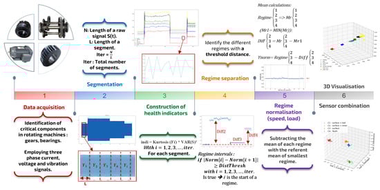
Figure 1.
Proposed methodology for fault detection and diagnostics under variable conditions.
2.1. Data Acquisition
In bearing and gear fault detection, several measurement types are used separately in the literature. Among them, vibration, current and voltage signals. In the case of gearbox monitoring, three-phase current and three-phase voltage signals carried out from the motor supply inverter are utilised. In addition to that, through experimentation analysis, voltage signals were found to be sensitive to speed variations while current signals are sensitive to both load and speed changes which gives the most amount of information about the system. In the case of variable regimes, they require a normalization in the health indicator to be able to work with these types of signals. Furthermore, the use of a vibration sensor placed in the proximity of the gearbox parts adds complexity but enables a better representation as it can evaluate the severity of the faults. This updated way of representing health states leads to a more accurate diagnostic.
2.2. Data Segmentation
In condition monitoring, segmentation is required to create data segments either through small data collection durations or by partitioning the full−length signal into segments for feature extraction. The goal is to extract one piece of useful information that represents the ensemble observations in the segment. Moreover, reducing the size of processed signals yields faster execution time as well as a simple representation of the system with negligible information loss. Thus, this step consists of taking the full length of a raw signal and transforming it into several segments with length L, as expressed in Equation (1).
where is the ith segment with represents the index of each segment. This latter variable can be calculated using Equation (2).
where N is the length of the total raw signal , and L is the length of the segment which is introduced manually after an empirical study. This length L impacts the amount of information extracted from the signal. In this study, choosing smaller L lengths results in more segments, which adds complexity to the process but increases the precision of this signal representation and is equal to 50,000 samples.
2.3. Health Indicator Construction
After signal segmentation, the next step consists of extracting statistical information from each segment, which allows the extraction of hidden information about the system’s health state. Then, the extracted features can be used as direct HI or combined to build a new one, enhancing fault detection performance. In this context, this paper uses powerful HI that combines two statistical features with high moment order. This HI is presented in Equation (3) uses kurtosis and variance [31].
Before the application of the HI product equation, the kurtosis function is first explored on some signals of a current phase belonging to different gearbox health states including gear, bearing and combined faults. It corresponds to estimating the extremity of deviations in each segment . In other terms, it measures the impulsive nature of a signal, as shown in Figure 2.
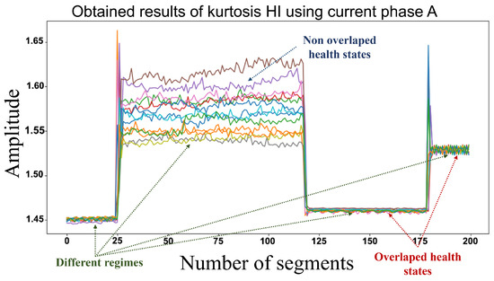
Figure 2.
Obtained results of kurtosis HI using current signal IA of different health states.
From this figure, the use of only kurtosis as HI shows that different regimes are highlighted, while the different system health states overlap in some regimes and do not overlap in others. Therefore, the variance function used in the HI generates a separation based on the amount of dispersion that exists in each health state. Hence, the product of kurtosis of each segment with the squared variance of the total signal allows separating each system state to its corresponding variation caused by faults while keeping regimes separation highlighted as shown in Figure 3.
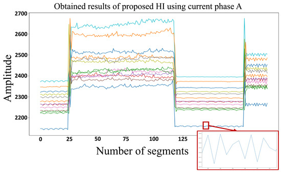
Figure 3.
Health indicator construction of a current phase.
Moreover, this HI will be applied not only on current phases but also on voltage and vibration signals with the same results.
2.4. Regime Separation and Normalization
2.4.1. Variable Regime Separation
The constructed HI in the previous subsection aims at separating the different health states, but overlapping in transient parts between regime change is always present. For this purpose, these regimes should be normalized, and first, pass through regime separation. This latter step implies a prior understanding of the intervals that represent each regime, i.e., identifying the exact time index where each regime starts and when it is finished. Therefore, this procedure begins by ranging the HI amplitude between zero and 1, which is only for the purpose of this index extraction using Equation (5):
Note that this range amplitude resizing allows only obtaining one threshold to identify regime index times. Then, through Equation (6) the starting index of each regime can be identified with respect to the threshold named DistThresh. Equation (6) expresses the absolute value of the difference between and to obtain a distance. When the result of this distance is greater than DistThresh, the index i is considered as a new regime start, and thus deduces the end of the previous regime. Hence, intervals of each regime can be identified and are marked as (, , , ,…) as in Figure 4.
with is the total number of segments.
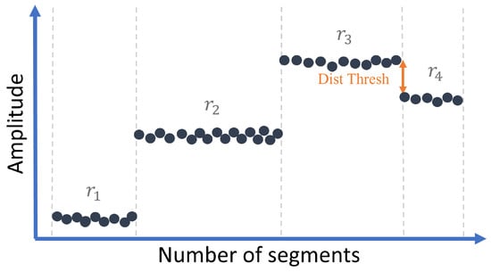
Figure 4.
Illustration of regime separation using a threshold.
The value is defined as the smallest distance between two consecutive regimes. For example, in the case of Figure 4, the threshold must be chosen as a value less than the value of the distance between and , which is the smallest distance between two consecutive regimes. Note that the existence of peaks before each regime is generated by the even window length of segmentation, and in this case it helps the regime separation function to distinguish the different regimes.
2.4.2. Regime Normalization
As shown in Figure 5, it can be observed that the HI belonging to the same health states presents different levels of amplitude due to the regime variation. In this subsection, and thanks to the identified regime indices, the regimes of each HI will be normalized.
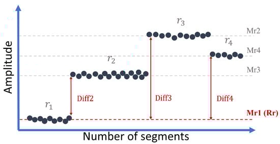
Figure 5.
Illustration of referent regime and mean calculation.
The normalization depends mainly on the manipulation of the average value of each regime. First, a referent value is calculated for the entire HI for normalization which is of the first regime. The choice of this regime is motivated by the fact that in theory, the starting regime of an induction motor starts with low speed knowing beforehand that the speed will increase over time. Also, current phases represent this behaviour change in speed better than voltage or vibration signals. As a result, based on current signals, the referent regime can be determined and applied to voltage and vibration HI for regime normalization.
In more detail, the manipulation of the mean values begins with Equation (7) by calculating the mean value of each regime in the health indicator, without the normalization between zero and one.
With and intervals acquired in the separation step. The result is the mean values of each regime , respectively.
To check the hypothesis of the referent regime. The lowest mean value in the health indicator needs to be the first mean value. In this case, is the lowest among the different regimes, which indicates that the referent regime () is the first variation in speed and load ().
The next step consists of using Equation (8) to calculate the difference between the referent regime and the mean values of the other regimes.
These differences in mean values are shown in Figure 5. To normalize these regimes, these differences (diffi) are subtracted from each corresponding regime (). Finally, normalized health indicators in current, voltage and vibration signals are obtained through a reconstruction with Ynorm:
As shown in Figure 6, the goal of regime normalization is to obtain a health indicator (Ynorm) as if data acquisition was conducted under constant operating conditions (constant speed and load).
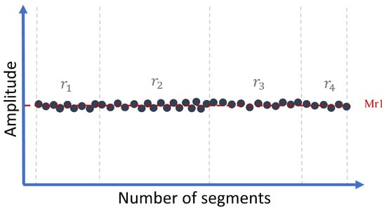
Figure 6.
Illustration of normalized regimes.
2.5. System Health State Signature
2.5.1. Three-Dimensional Visualisation
Figure 7, Figure 8, Figure 9 and Figure 10 shows a three-dimensional (3D) representation of the health indicators with normalized regimes (Equation (9)). Figure 7 is a representation of the three current phases (Ia, Ib, Ic). Figure 8 with voltage phases (Va, Vb, Vc). Figure 9 represents vibration signals with kurtosis, variance and root mean square functions. Lastly, Figure 10 shows combined current, voltage phases and vibration signals. These health indicators belong to four different health states, Gear surface damage (C1) and a Broken gear tooth (C2), as well as two combined faults (C3: Gear surface damage + Inner race bearing fault, C4: Gear surface damage + Outer race bearing fault). These results are obtained after the normalization of four different regimes (1500 rpm at 50% load for 50 s, 2800 rpm at 100% load for 3 min, 1500 rpm at 100% load for 2 min and 1000 rpm at 0% load for 1 min).
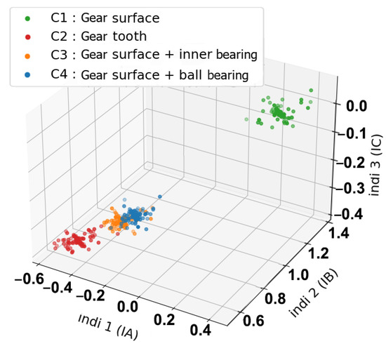
Figure 7.
Three-dimensional representation of health indicator using current signals.
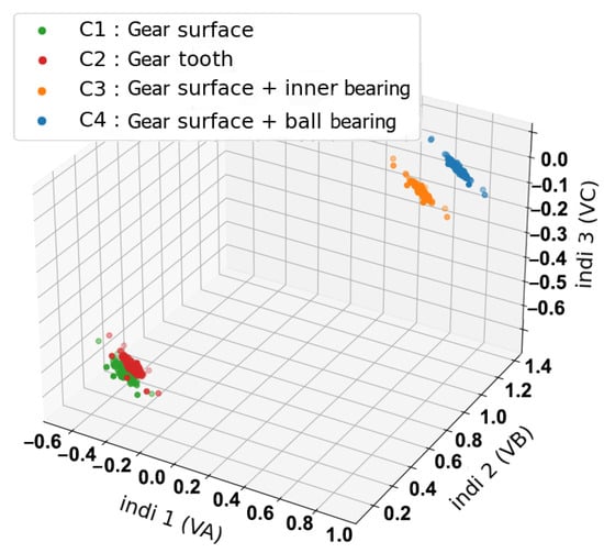
Figure 8.
Three-dimensional representation of health indicator using voltage signals.
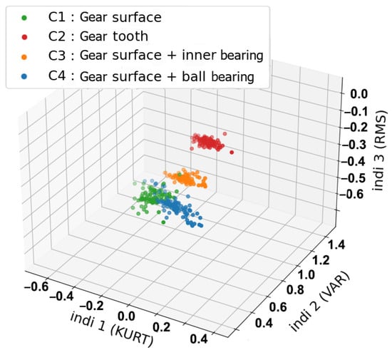
Figure 9.
Three-dimensional representation of vibrations health indicators using Kurt, Var and RMS values.
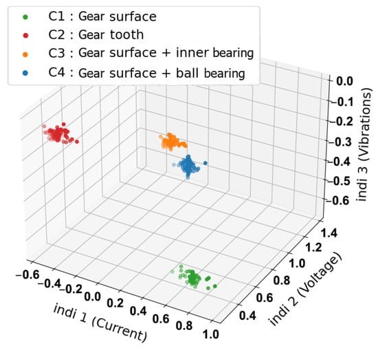
Figure 10.
Sensor combination of current, voltage and vibration signals.
2.5.2. Sensor Combination
As seen in Figure 7, Figure 8 and Figure 9, the use of separated sensors as in 3D representations with only current phases, voltage phases or vibration signals leads to confusion (overlapping) between the observations of different health states. In the current indicators (Figure 7), an overlapping is located between the combined faults C4, and combined faults C3. In the voltage indicators (Figure 8), an overlapping can be shown between C1 and C2. Even in Figure 9, we can see that a combination of the well-known statistical indicators (RMS, kurtosis and variance) in the vibration signals shows an overlapping between C1 and C4. This issue is present due to faults sharing similar properties and characteristics, which leads to observations with similar values. As a consequence, applying fault diagnosis with this amount of confusion will result in losing precision as well as misidentifying classes. To resolve this issue, a sensor combination is introduced. This combination includes merging three current phases into one representative signal, and voltage phases into one signal (Equation (10)). With the help of vibrations, each health state can then be represented with current, voltage and vibrations in the same representation space. This combination creates a representation without any visible overlapping even in the case of combined faults as shown in Figure 10.
2.6. Fault Classification
The objective of this step is to detect and diagnose faults in the system by employing a classification approach using the normalized regime HI [32]. The classification aims to determine the appropriate class of new HI observations from a set of historical HI classes (, etc.) such as healthy, faulty type 1, fault type 2, etc.
In the literature, there exist numerous techniques for classification. One can cite the most used ones, Support Vector Machine (SVM) [23], Random Forest (RF) [33], K-Nearest Neighbors (K-NN) [34], Naive Bayes (NB) [35]. In this study, a new geometrical classifier tool is proposed. However, before this latter step, the data should be prepared and structured. In general, the data are split into training and testing data sets. Hence, the normalized regime HI is split 50% for training and 50% for testing. The training set is organized by a matrix of n lines of HI observations of all health states after regime normalization. Four columns corresponding to combined current phases, combined voltage phases, vibration, and a last column that represents the health index of the system (Labels ), with m the number of classes. After that, as the current, voltage and vibration are heterogeneous measurements, they are normalized to their dispersion using Equation (11). The calculated and values of the training set are used to normalize the test set (Equation (12)). Finally, the train set is injected into classifiers for learning.
With , as the normalized data sets, the desired results for classification models are illustrated in Figure 11, which represents the impact of regime normalization on the dispersion of health states. Contrary to Figure 12, which represents the classification conditions without regimes normalization.
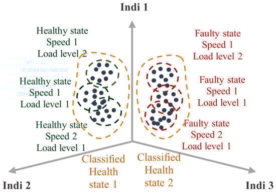
Figure 11.
Representation of the class classification desired without overlapping.
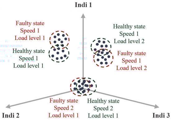
Figure 12.
Representation of the class classification obtained with overlapping.
In this paper, we propose a new statistical classifier named geometrical classification (GC) for robust fault diagnostics. This tool uses first a K-means clustering [24] to calculate the gravity centroid (G) that represents each health state. The purpose of these centroids is to determine an average distance between the observations of a class using Equation (13).
where is the number of segments in each class , and is the centroid of these classes. This average distance then is used to calculate the peripheral threshold of that class with Equation (14).
Using the calculated centroids and their average distances, peripheral thresholds are created for each class. It creates a 3D spherical space (see Figure 13) that helps decision making for the classification of new observations and is calculated using Equation (14).
where is the standard deviation of the classes. This peripheral threshold allows us to define the extremities of that class.
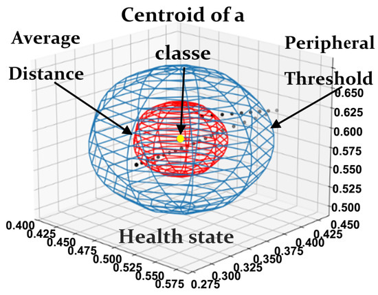
Figure 13.
Different parameters of a health state in geometrical classification.
According to this procedure, once new observations are acquired , their centroid is computed. Subsequently, the distance between this centroid and the existing historical centroids is assessed (Equation (15)).
where m and n are the number of classes. In such a scenario, if the distance value is below the peripheral threshold for a particular class, it indicates that the current health state of the system corresponds to that class.
For instance, let us assume that () is the healthy state of the system; if the distance between the centroid of a new case () is lower than the peripheral threshold of the class (), it is directly identified as a healthy state. If the calculated distance does not belong to any peripheral threshold, a new health state is detected as shown in Figure 14. Therefore, this approach can help to enhance the training data set and improve it by adding more classes, which represent unknown health states of this system, as shown in the following Algorithm 1.
| Algorithm 1: Proposed geometrical classification algorithm |
1: Load training data set in and it’s labels, train 2: Load testing data set in and it’s labels, test 3: Import K-means library 4: Determine centroids of train, and save in G 5: Set the number of classes in training set, m 6: Set the number of observations in a class, iter 7: for k = 1 to m do 8: for j = 1 to iter do 9: Calculate distance between and , save in 11: Calculate the average distance of , save in 12: Calculate the peripheral threshold of , save in 14: Set the number of classes in training set, n 15: Determine centroids of test, and save in 16: for i = 1 to n do 17: for j = 1 to m do 18: Calculate distance between and , save in 19: Look for the minimal distance in , and save in 20: if do 21: Label as the class in the train set 22: else Create new class N |
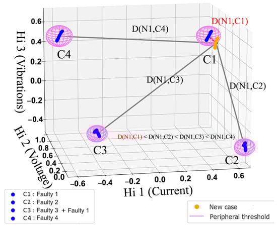
Figure 14.
A demonstration of the GC algorithm application.
3. Application and Results
This section presents the application used to verify the performance of the proposed methodology for bearing and gear fault detection and diagnostics under variable regimes. The application consists of a test bench installed in a laboratory (see Figure 15). The test bench used three-phase current, three-phase voltage and vibration data continuously recorded at different operating regimes (varying the speed and the load in each data acquisition). The latter data are processed separately and then combined after HI construction. Moreover, a comparison between classical techniques and the proposed methodology is investigated to highlight the limits of the traditional one and to emphasize the added value of the proposed methodology. Finally, the obtained results are evaluated through an accuracy diagnostic metric.
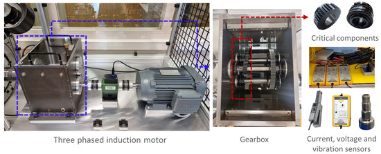
Figure 15.
Test bench installed at LASPI laboratory.
3.1. Case Study and Data Description
The test bench is dedicated to the study of fault detection and diagnosis of bearing and gear components and is installed at the LASPI laboratory in France. It is composed of an induction motor, which drives a gearbox of three shafts. Each shaft contains bearing and gear components. At the end of this gearbox, an electromagnetic powder brake is placed to apply a load level to the motor (Figure 16). National Instrument acquisition devices (NI9234) are used to collect the data. Three current and three voltage sensors are carried out from the inverter output while an accelerometer is placed on the gearbox side as close as possible to the rotating shaft. The acquired data parameters correspond to a duration of 6 min and 50 s per experiment with a sampling frequency of 25.6 KHz.
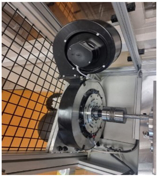
Figure 16.
Electromagnetic brake.
In total, 13 were experiments achieved, where each one presents four load levels and four speed variations, starting with 50% load at 1500 rpm for 50 s, 100% load at 2800 rpm for 3 min, 100% load at 1500 rpm for 2 min and 0% load at 1000 rpm for 1 minute. All these parameters are summarized in Table 1 and Figure 17.

Table 1.
Operational conditions of the tests applied in LASPI platform.
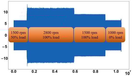
Figure 17.
Raw current phase signal.
From this table, each experiment presents a specified health state of a component. It is equipped with specific bearings and gears with healthy and different fault states such as outer-, inner- and ball-bearing faults and gears with half-tooth faults, tooth breaks and gear-surface damage. An overall scheme of the test bench is presented in Figure 18 which highlights the different parameters of the gearbox system.
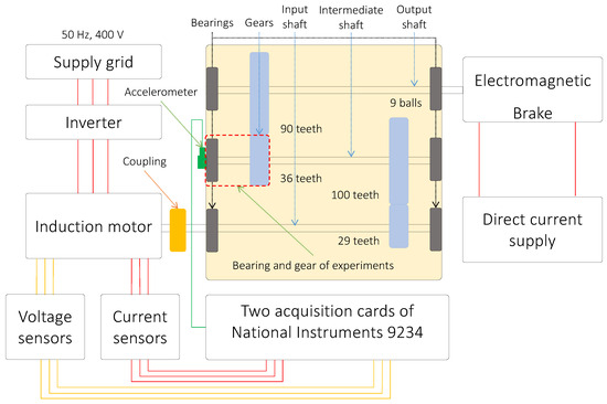
Figure 18.
Representation of the parameters in LASPI gearbox system.
The next subsection aims to present data prepossessing and the obtained results of the methodology steps with a comparison of the HI results with regime normalization and without regime normalization.
3.1.1. Segmentation
To process the acquired data, the first step is the segmentation to split every signal into a number of segments (iter) of length L. Each recorded signal is equal to 6 min and 50 s and is split into 205 segments of 2 s each (L = 2 s, iter = 205).
3.1.2. Health Indicator Construction
In this application, thirteen experimental tests where performed with different operating regimes in the same data acquisition of the three current and voltage phases as well as vibration signals. With these data, health indicators (HI) are then constructed to evaluate the performance and the robustness of the methodology proposed in Section 2.
3.2. Application and Results of the Classical and Proposed Approach
3.2.1. Classical Methods
The conventional method consists of constructing health indicators from signals using Equation (4) as shown in Figure 19, Figure 20, Figure 21 and Figure 22. This is a method that has proven to be robust for fault detection and diagnosis of bearing and gear faults under constant operating conditions. However, when introducing variable regimes, we can clearly see the overlap between the different health states where it is very difficult to distinguish classes. Even in traditional health indicators, such as kurtosis in Figure 23, RMS in Figure 24 and variance in Figure 25; when they are used frequently in condition monitoring, they exhibit even more overlapping between the health states. Due to the variable regimes, with different loads and speeds, these figures show a wide dispersion and an intersection of the different parts that represent the health states. Thus, one can conclude that their use is not sufficient and it is not possible to diagnose defects as it will be highlighted in the fault classification.
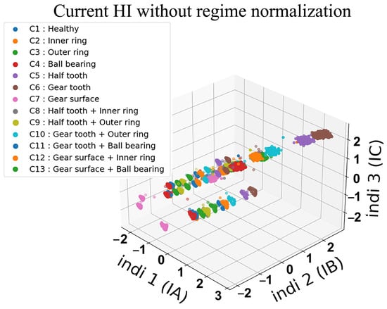
Figure 19.
Classical three-dimensional representation of HI with three current phases without regime normalization.
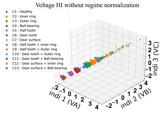
Figure 20.
Classical three-dimensional representation of HI with three voltage phases.
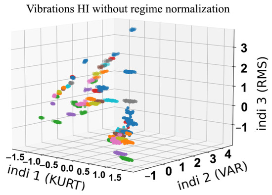
Figure 21.
Classical three-dimensional representation of HI with vibration signals.
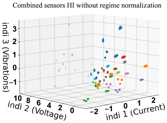
Figure 22.
Classical three-dimensional representation of HI with current, voltage and vibration.
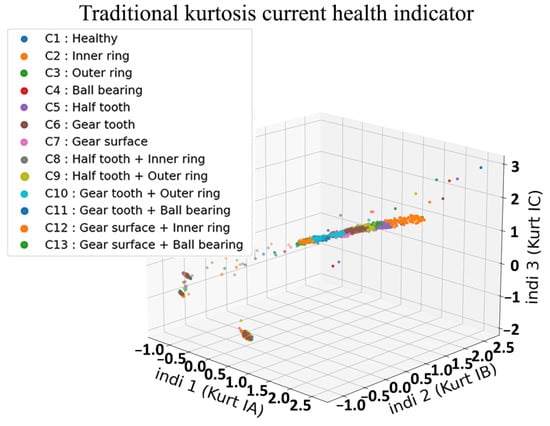
Figure 23.
Classical three-dimensional representation of kurtosis HI with three current phases.
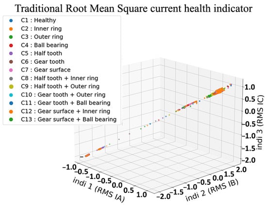
Figure 24.
Classical three-dimensional representation of RMS HI with three current phases.
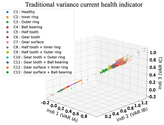
Figure 25.
Classical three-dimensional representation of variance HI with three current phases.
3.2.2. Proposed Method
The newly proposed method consists of constructing health indicators from current, voltage and vibration signals using Equation (4) in Section 2.3, similar to the classical method. Then, a separation step is applied using a threshold to identify the different regimes. A referent regime (Rr) is identified as having the lowest mean value in the data acquisition, and the regimes are normalised to the mean value of this Rr in the current, voltage and vibration signals as shown in Figure 26, Figure 27 and Figure 28. From Figure 29, Figure 30 and Figure 31, it can be seen that the proposed methodology can clearly separate thirteen classes corresponding to the different health states of our gearbox system.
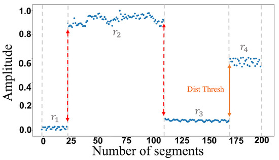
Figure 26.
Regime identification.
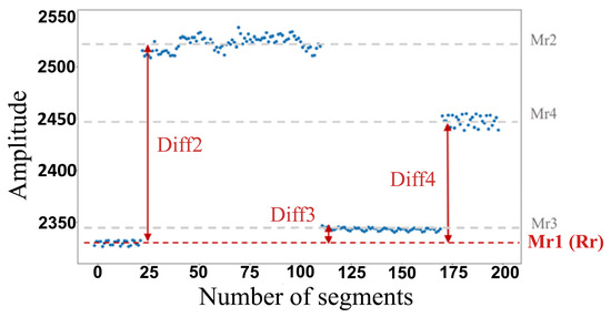
Figure 27.
Regime mean normalization.
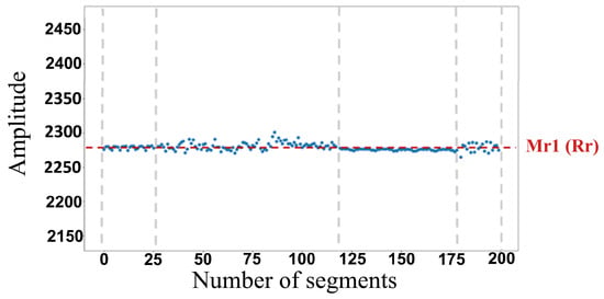
Figure 28.
Normalization results.
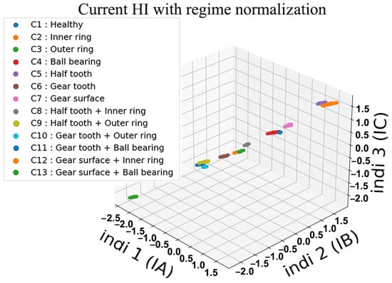
Figure 29.
Proposed three-dimensional representation of HI with three current phases.
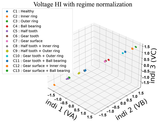
Figure 30.
Proposed three-dimensional representation of HI with three voltage phases.
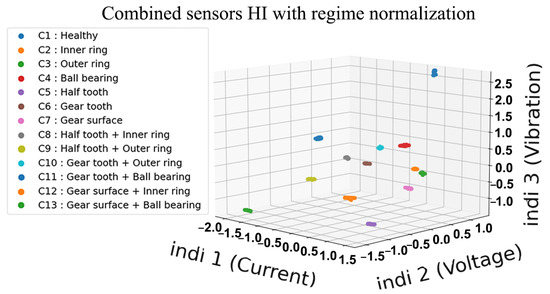
Figure 31.
Proposed three-dimensional representation of HI with current, voltage and vibrations.
This representation is not affected by the multiple changes in load and speed levels within the same data acquisition. Also, this class distinction can be seen in current as well as in voltage health indicators. Nonetheless, the true separation of these classes is a result of the three sensors combined in Figure 31. This combination makes it possible to identify not only the different classes but also the combined ones sharing a type of fault. In other terms, these combined classes tend to be very close and hard to distinguish because they have similar characteristics. Therefore, these results highlight the efficiency of the proposed regime normalization to solve the health states overlapping under variable operating regimes, even in the cases of combined bearing and gear faults.
3.3. Fault Classification
The health indicators extracted previously are used in this subsection for bearing and gear fault diagnosis. For this purpose, these health indicators are fed into the input of multiple ML models. Moreover, the data are divided into a training set and a testing set, both are composed of random parts of each regime from the total observations. In order to prove the efficiency of the method, both supervised and unsupervised ML were employed. The supervised classification includes models such as Support Vector Machine (SVM), Random Forest (RF), K-Nearest Neighbor (KNN) and Naive Bayes (NV). The classification was applied to health indicators from the classical method without regime normalization, and compared with indicators from the proposed method. Furthermore, this approach was applied to the thirteen different health states () which represent the majority of the faults which can be found in such systems. Therefore, it is necessary to be able to train a classifier that can diagnose not only bearing and gear faults but combined faults which can be harder to distinguish.
After all, Table 2 summarizes the results obtained from the supervised classification of the classical method. One can notice very low results with no classifier being able to identify one health state at 100% accuracy. SVM achieved a very low accuracy of 8%, with ten faults completely missed, and the most observations correctly classified in one class at 35%, which represents less than half the observations in a class. Similarly, Random Forest had the highest accuracy of 37%. Additionally, the combined faults were the classes with the lowest overall accuracy. In other terms, the fault diagnostics which solely rely on the accuracy of the classifiers will suffer from false health state identifications with these types of results.
Table 2.
Supervised classification with the proposed health indicators and non normalized regimes using 3D current, voltage and vibration representation.
By contrast, based on Table 3 which represents results obtained by classifying health indicators with normalized regimes, one can notice that three out of the four classifiers managed to achieve accuracy with every observation in all the different classes correctly classified. Expect the NF model which achieved an overall accuracy of 92%. Moreover, not only were the different heath states classified, but even combined faults, which tend to be harder to distinguish, were managed.
Table 3.
Supervised classification with the proposed health indicators and Normalized regimes using 3D current, voltage and vibration representation.
These results highlight the superiority of the proposed method in fault classification over the classical method using supervised ML and show that even with influence from variable regimes on the system, fault diagnosis can be performed with simple and fast tools. The only shortcoming of supervised ML is the need for relatively large data sets and it does not have the ability to update these data sets. For this purpose, a different approach is proposed called the geometrical classification (GC) algorithm. This approach includes an unsupervised ML model with geometrical techniques for fault diagnosis (Section 2.6).
When applying this approach to the classical methods of health indicator construction. The first step of determining the centroids of each class with a clustering model (K-means) failed. K-means clustering was not able to determine the classes that need to be clustered. This failure is a consequence of the amount of overlap between the health states induced by the variable regimes (Figure 22).
Alternatively, when applying the health indicators from the proposed method with normalized regimes, results were obtained and illustrated in Table 4. These results represent the accuracy between the labels generated by the model and the existing labels of the test sets. As it is clearly seen, the model successfully clustered and labelled the observations according to their respective classes and health states. This precision includes the ability to identify new health states to add to the existing data sets (Figure 32), with the mission of avoiding false diagnostics and increasing reliability.
Table 4.
Unsupervised geometrical classification with the proposed health indicators and normalized regimes using 3D current, voltage and vibration representation.
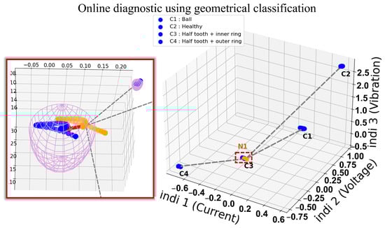
Figure 32.
New health state in geometrical classification.
According to the findings in Table 3 and Table 4, the proposed methodology has significantly enhanced the accuracy of class predictions under variable environmental conditions, outperforming state-of-the-art methods, particularly evident in the results of combined fault classes. This advancement is primarily attributed to integrating HI fusion and regime normalization. However, it is essential to acknowledge certain limitations:
- Computational resources and time: Implementing multiple processing steps for HI construction requires considerable computational resources, which may lead to longer durations for diagnostic analysis.
- Data quality and quantity: As with other supervised learning approaches, the effectiveness of model training hinges on the availability of ample high-quality data. Deficiencies in the data set can compromise the accuracy of the predictions.
- Variability of operating conditions between different failure modes: The proposed scenario, which includes several failure modes, poses a significant problem, particularly in cases where faults are combined and may lead to fault alarms. A potential improvement could be to introduce a probability function into the classification results, which can help separate the system state in cases where the class of a single fault is clustered with the class of a combined fault.
4. Conclusions
In this paper, a methodology based on electrical and vibration signals has been presented for the detection and diagnostics of bearings and gears under variable regimes. First, segmentation of the signals was performed to extract a set of relevant features. These features were combined to construct a health indicator based on the impulsive properties of segments, and the amount of dispersion that exists in each heath state. With the help of the proposed separation and normalization of regimes, each health state grouping multiple regimes was distinguished. Finally, the normalized regime’s health indicators were used by classifiers for the detection and diagnostics. The proposed methodology was tested on experimental data that highlighted the separability of different health states of the system including bearing, gear and combination of bearing and gear faults simultaneously. Among classifiers, a geometric classification method was proposed that could classify known and unknown classes. In future endeavours, we aim to explore advanced health indicator construction with automatic parameter definitions, such as data segmentation length, to enhance the methodology resilience across diverse operational conditions. We also intend to add a probability layer in the prediction such as fuzzy logic to enhance the clustering of new unknown health states that could be confused with historical ones. These efforts are directed towards continually advancing the predictive capabilities and applicability of the proposed methodology.
Author Contributions
Conceptualization, M.B. and M.S.; methodology, M.B.; software, M.B.; validation, M.S., A.S. and H.R.; formal analysis, M.S.; investigation, M.B.; resources, M.S., A.S. and H.R.; data curation, M.S.; writing—original draft preparation, M.B.; writing—review and editing, M.B., M.S., A.S. and H.R.; visualization, M.B.; supervision, M.S.; project administration, A.S. and H.R.; All authors have read and agreed to the published version of the manuscript.
Funding
This research received no external funding.
Data Availability Statement
The datasets presented in this article are not readily available because the data are part of an ongoing study.
Conflicts of Interest
The authors declare no conflicts of interest.
References
- Çınar, Z.M.; Abdussalam Nuhu, A.; Zeeshan, Q.; Korhan, O.; Asmael, M.; Safaei, B. Machine learning in predictive maintenance towards sustainable smart manufacturing in industry 4.0. Sustainability 2020, 12, 8211. [Google Scholar] [CrossRef]
- Castellani, F.; Garibaldi, L.; Daga, A.P.; Astolfi, D.; Natili, F. Diagnosis of faulty wind turbine bearings using tower vibration measurements. Energies 2020, 13, 1474. [Google Scholar] [CrossRef]
- Imani, M.B.; Heydarzadeh, M.; Khan, L.; Nourani, M. A scalable spark-based fault diagnosis platform for gearbox fault diagnosis in wind farms. In Proceedings of the 2017 IEEE International Conference on Information Reuse and Integration (IRI), San Diego, CA, USA, 4–6 August 2017; pp. 100–107. [Google Scholar]
- Kumar, A.; Gandhi, C.; Zhou, Y.; Kumar, R.; Xiang, J. Latest developments in gear defect diagnosis and prognosis: A review. Measurement 2020, 158, 107735. [Google Scholar] [CrossRef]
- Vasic, M.; Stojanovic, B.; Blagojevic, M. Fault analysis of gearboxes in open pit mine. Appl. Eng. Lett. J. Eng. Appl. Sci. 2020, 2, 50–61. [Google Scholar] [CrossRef]
- Jablonski, A.; Dworakowski, Z.; Dziedziech, K.; Chaari, F. Vibration-based diagnostics of epicyclic gearboxes–From classical to soft-computing methods. Measurement 2019, 147, 106811. [Google Scholar] [CrossRef]
- Kundu, P.; Darpe, A.K.; Kulkarni, M.S. A review on diagnostic and prognostic approaches for gears. Struct. Health Monit. 2021, 20, 2853–2893. [Google Scholar] [CrossRef]
- Vencl, A.; Gašić, V.; Stojanović, B. Fault tree analysis of most common rolling bearing tribological failures. In Proceedings of the IOP Conference Series: Materials Science and Engineering, Galati, Romania, 22–24 September 2016; IOP Publishing: Bristol, UK, 2017; Volume 174, p. 012048. [Google Scholar]
- Gougam, F.; Rahmoune, C.; Benazzouz, D.; Merainani, B. Bearing fault diagnosis based on feature extraction of empirical wavelet transform (EWT) and fuzzy logic system (FLS) under variable operating conditions. J. Vibroengineering 2019, 21, 1636–1650. [Google Scholar] [CrossRef]
- Helmi, H.; Forouzantabar, A. Rolling bearing fault detection of electric motor using time domain and frequency domain features extraction and ANFIS. IET Electr. Power Appl. 2019, 13, 662–669. [Google Scholar] [CrossRef]
- Kafeel, A.; Aziz, S.; Awais, M.; Khan, M.A.; Afaq, K.; Idris, S.A.; Alshazly, H.; Mostafa, S.M. An Expert System for Rotating Machine Fault Detection Using Vibration Signal Analysis. Sensors 2021, 21, 7587. [Google Scholar] [CrossRef] [PubMed]
- Soualhi, M.; Nguyen, K.T.; Soualhi, A.; Medjaher, K.; Hemsas, K.E. Health monitoring of bearing and gear faults by using a new health indicator extracted from current signals. Measurement 2019, 141, 37–51. [Google Scholar] [CrossRef]
- Soualhi, M.; Nguyen, K.T.; Medjaher, K. Pattern recognition method of fault diagnostics based on a new health indicator for smart manufacturing. Mech. Syst. Signal Process. 2020, 142, 106680. [Google Scholar] [CrossRef]
- Zamudio-Ramirez, I.; Saucedo-Dorantes, J.J.; Antonino-Daviu, J.; Osornio-Rios, R.A.; Dunai, L. Detection of Uniform Gearbox Wear in Induction Motors Based on the Analysis of Stray Flux Signals Through Statistical Time-Domain Features and Dimensionality Reduction Techniques. IEEE Trans. Ind. Appl. 2022, 58, 4648–4656. [Google Scholar] [CrossRef]
- Altaf, M.; Akram, T.; Khan, M.A.; Iqbal, M.; Ch, M.M.I.; Hsu, C.H. A new statistical features based approach for bearing fault diagnosis using vibration signals. Sensors 2022, 22, 2012. [Google Scholar] [CrossRef] [PubMed]
- Medjaher, K.; Zerhouni, N.; Gouriveau, R. From Prognostics and Health Systems Management to Predictive Maintenance 1: Monitoring and Prognostics; John Wiley & Sons: Hoboken, NJ, USA, 2016. [Google Scholar]
- Zhou, L.; Duan, F.; Mba, D.; Wang, W.; Ojolo, S. Using frequency domain analysis techniques for diagnosis of planetary bearing defect in a CH-46E helicopter aft gearbox. Eng. Fail. Anal. 2018, 92, 71–83. [Google Scholar] [CrossRef]
- Sharma, V.; Parey, A. A review of gear fault diagnosis using various condition indicators. Procedia Eng. 2016, 144, 253–263. [Google Scholar] [CrossRef]
- Dhamande, L.S.; Chaudhari, M.B. Compound gear-bearing fault feature extraction using statistical features based on time-frequency method. Measurement 2018, 125, 63–77. [Google Scholar] [CrossRef]
- Feng, Z.; Zhu, W.; Zhang, D. Time-Frequency demodulation analysis via Vold-Kalman filter for wind turbine planetary gearbox fault diagnosis under nonstationary speeds. Mech. Syst. Signal Process. 2019, 128, 93–109. [Google Scholar] [CrossRef]
- Damine, Y.; Bessous, N.; Pusca, R.; Megherbi, A.C.; Romary, R.; Sbaa, S. A New Bearing Fault Detection Strategy Based on Combined Modes Ensemble Empirical Mode Decomposition, KMAD, and an Enhanced Deconvolution Process. Energies 2023, 16, 2604. [Google Scholar] [CrossRef]
- Sarker, I.H. Machine learning: Algorithms, real-world applications and research directions. SN Comput. Sci. 2021, 2, 1–21. [Google Scholar] [CrossRef]
- Goyal, D.; Choudhary, A.; Pabla, B.; Dhami, S. Support vector machines based non-contact fault diagnosis system for bearings. J. Intell. Manuf. 2020, 31, 1275–1289. [Google Scholar] [CrossRef]
- Manikandan, S.; Duraivelu, K. Fault diagnosis of various rotating equipment using machine learning approaches–A review. Proc. Inst. Mech. Eng. Part J. Process. Mech. Eng. 2021, 235, 629–642. [Google Scholar] [CrossRef]
- Saufi, S.R.; Ahmad, Z.A.B.; Leong, M.S.; Lim, M.H. Challenges and opportunities of deep learning models for machinery fault detection and diagnosis: A review. IEEE Access 2019, 7, 122644–122662. [Google Scholar] [CrossRef]
- Tao, H.; Wang, P.; Chen, Y.; Stojanovic, V.; Yang, H. An unsupervised fault diagnosis method for rolling bearing using STFT and generative neural networks. J. Frankl. Inst. 2020, 357, 7286–7307. [Google Scholar] [CrossRef]
- Li, Y.; Geng, C.; Zuo, M.J.; Liang, X. Use of vibration signal to estimate instantaneous angular frequency under strong nonstationary regimes. Mech. Syst. Signal Process. 2023, 200, 110571. [Google Scholar] [CrossRef]
- Ma, Q.; Yang, J. Motor Bearing Fault Diagnosis in an Industrial Robot Under Complex Variable Speed Conditions. J. Comput. Nonlinear Dyn. 2024, 19, 021007-1. [Google Scholar]
- Hasan, M.J.; Kim, J.M. Bearing fault diagnosis under variable rotational speeds using stockwell transform-based vibration imaging and transfer learning. Appl. Sci. 2018, 8, 2357. [Google Scholar] [CrossRef]
- Yang, X.; Zhou, P.; Zuo, M.J.; Tian, Z. Normalization of gearbox vibration signal for tooth crack diagnosis under variable speed conditions. Qual. Reliab. Eng. Int. 2022, 38, 3072–3098. [Google Scholar] [CrossRef]
- Liu, Z.; Zhang, L. A review of failure modes, condition monitoring and fault diagnosis methods for large-scale wind turbine bearings. Measurement 2020, 149, 107002. [Google Scholar] [CrossRef]
- Zhang, J.; Zhang, Q.; Qin, X.; Sun, Y. A two-stage fault diagnosis methodology for rotating machinery combining optimized support vector data description and optimized support vector machine. Measurement 2022, 200, 111651. [Google Scholar] [CrossRef]
- Han, T.; Jiang, D.; Zhao, Q.; Wang, L.; Yin, K. Comparison of random forest, artificial neural networks and support vector machine for intelligent diagnosis of rotating machinery. Trans. Inst. Meas. Control. 2018, 40, 2681–2693. [Google Scholar] [CrossRef]
- Baraldi, P.; Cannarile, F.; Di Maio, F.; Zio, E. Hierarchical k-nearest neighbours classification and binary differential evolution for fault diagnostics of automotive bearings operating under variable conditions. Eng. Appl. Artif. Intell. 2016, 56, 1–13. [Google Scholar] [CrossRef]
- Wu, Y.; Fu, Z.; Fei, J. Fault diagnosis for industrial robots based on a combined approach of manifold learning, treelet transform and Naive Bayes. Rev. Sci. Instrum. 2020, 91, 015116. [Google Scholar] [CrossRef] [PubMed]
Disclaimer/Publisher’s Note: The statements, opinions and data contained in all publications are solely those of the individual author(s) and contributor(s) and not of MDPI and/or the editor(s). MDPI and/or the editor(s) disclaim responsibility for any injury to people or property resulting from any ideas, methods, instructions or products referred to in the content. |
© 2024 by the authors. Licensee MDPI, Basel, Switzerland. This article is an open access article distributed under the terms and conditions of the Creative Commons Attribution (CC BY) license (https://creativecommons.org/licenses/by/4.0/).