Driving Profile Optimization for Energy Management in the Formula Student Técnico Prototype

Abstract

This study addresses the challenge of optimizing energy management in the electric vehicle industry, specifically focusing on motorsport. It particularly targets optimizing energy management during an endurance event at the Formula Student competition. The research involves detailed simulation of a complete endurance event, including developing precise track and vehicle models and their application in real-time energy management of our motorsport vehicle. The primary objective is to develop an energy reference profile that optimizes point scoring following the event’s specific rules. The energy reference profile serves as a strategic guideline for energy consumption and its regeneration throughout the endurance event. What sets this study apart is its emphasis on the real-time feedback controller’s implementation in the Formula Student prototype, FST12, specifically during the endurance event. This controller dynamically regulates the inverter’s power output, ensuring the vehicle closely follows the pre-established energy reference profile. This real-time energy management approach enhances overall performance by optimizing energy utilization for maximum scoring potential. The developed distance estimation method presented an error of less than 0.7% compared to experimental measurements. The Formula Student prototype, FST12, underwent experimental validation on a real 20 km closed-loop track. Results showed that the optimized strategy can be implemented with less than 0.5% of error in energy consumption and 6.8% of error in the obtained competing points.

1. Introduction

Optimizing energy consumption is a significant challenge for both research and industrial communities. In electric vehicles, this challenge is aggravated due to the limited capacity of batteries, which ultimately limits the range and attractiveness of EVs [1]. Two current approaches to address this issue are the development of highly efficient powertrains and advancing energy use optimization techniques.

Regarding powertrains, one example is the use of multiple energy sources to reduce the limitation of the batteries [2]. Supercapacitors, flywheels, and fuel cells can be combined with batteries to improve the energy management of EVs [3,4]. The development of highly efficient electric motors [5] and powertrain optimization [6] are also other approaches to reducing energy consumption. In [7], for example, the authors presented the design optimization of an in-wheel permanent magnet synchronous motor to reduce the number of materials used and the weight compared to conventional motors, and in [8], the authors optimized a permanent magnet synchronous motor with a cobalt iron core.

The second issue addressed is energy management optimization algorithms, which offer a complementary approach to mitigating the limited capacity of batteries. In [9], an algorithm was proposed for intelligent transportation systems, utilizing an adaptive equivalent fuel consumption minimization strategy. This approach considers the battery’s state of charge and optimizes the vehicle’s start–stop function using NARX network-based velocity prediction. This method achieved fuel savings of up to 9%. In [10], the authors proposed a path and speed optimization strategy to extend the range of an electric unmanned marine vehicle (USV) powered by batteries and photovoltaic panels. Experimental tests demonstrated that the USV could be fully powered by PV panels under low speed and wave conditions, with path and speed optimizations increasing the range by up to 25%. In [11], an energy management strategy was proposed for hybrid electric buses considering thermal safety and degradation awareness for lithium-ion batteries, showing a mitigation of the battery aging by 34.8%. Real-time optimization techniques also play an important role in energy minimization, as shown in [12,13]. The authors showed that it is possible to use effective real-time cost-minimization power strategies based on model predictive control for hybrid electric vehicles.

Therefore, optimizing the driving profile is a crucial step in energy management. It must be tailored to the vehicle’s dynamics, weather, and road conditions to minimize energy consumption and maximize range while ensuring a minimum driving time. However, in a racing environment [14], the vehicle consumes significant energy to achieve maximum speed over the given track distance. In this critical context, this research focuses on developing energy management strategies for implementation in a racing Formula Student prototype.

Formula Student is Europe’s most established educational engineering competition, challenging engineering students from the best universities around the world to conceptualize, design, build, and test electric or combustion single-seater Formula race cars according to a specific set of rules [15]. FST Lisboa [16] was established in 2001 and is the Formula Student team from the University of Lisbon. Throughout its history, the team has strived to keep up with the industry’s ever-growing demands and advancements, first with the transition from combustion to electric in 2010 and then with the development of the team’s first autonomous car in 2021.

Formula Student competitions are divided into static and dynamic events. The static events assess each team’s knowledge and engineering processes. The dynamic events in the EV category include the following:

• Acceleration: a 75 m straight line to test the longitudinal acceleration capability.
• Skidpad: two pairs of concentric circles in a figure-eight pattern to test the lateral acceleration capability.
• Autocross: a single lap on a handling track with features such as hairpins, slaloms, and chicanes, approximately 1 km long.
• Endurance: a roughly 22 km closed-loop circuit with characteristics such as Autocross, including a driver change at the halfway point.
• Efficiency: evaluates the vehicle’s energy efficiency during the endurance event.

Endurance and efficiency events together account for 325 out of 1000 points, nearly a third of the total available points. During the testing season, the team has limited opportunities to simulate endurance events, as these tests can deplete an entire battery pack, or come close to it. Additionally, endurance events are the most challenging to perform consistently well in, requiring meticulous preparation in car reliability, driver training, and, most importantly, temperature and energy management. Being the most challenging event in last year’s FSG [17], only 13 EV teams successfully finished the endurance event (18% out of the 70 registered and 25% out of the 52 who started altogether).

The research began with the FST Lisboa team using a simple algorithm for energy management. Recognizing the lack of a robust controller to enhance overall performance in the endurance and efficiency events, the need for a more sophisticated system became evident, motivating this research. The ultimate objective is to develop methodologies to optimize energy use, increasing confidence in successfully completing the event and enhancing point-scoring opportunities. Regarding other solutions employed by different teams, there is very little official information due to competition purposes. However, during competitions, the students share information about their solutions. For example, the TU Munich team has devised a real-time strategy tool that predicts lap times and system temperatures during an endurance race, providing valuable information to the drivers. Also, the team from RWTH Aachen has developed a simulator that takes the track layout into account and conducts an endurance simulation. It identifies specific track segments where it is more advantageous for the driver to coast rather than continuously accelerate. This information is conveyed in real time by illuminating an LED on the dashboard, prompting the driver to ease off the throttle pedal to conserve energy. In [18], Formula Student Netherlands developed a convex optimization framework to compute the minimum-lap-time control strategy for their vehicle.

Following this topic, we propose a methodology to generate an optimized energy reference profile and implement it in real time. As such, a pre-event optimized plan is generated through a developed offline model and implemented into an energy management algorithm that adheres the actual energy deployment to what has been deemed optimal. The proposed methodology is validated on a real closed-loop track. Therefore, the core contribution of this paper is to develop a robust application of driving profile optimization to maximize the vehicle’s performance (in this case, defined by the score) during competitions in motorsport. This strategy presents two stages. First, it requires discretized detailed models of the vehicle and track, calibrated experimentally, to be used in energy optimization algorithms. Then, a real-time implementation is proposed, where the optimized driving profile is used to limit the output power from the motors while still providing the driver the control of the vehicle’s speed and maneuverability. To achieve real-time implementation, inertial measurement units and GPS measurements are used to estimate the vehicle’s real-time position. The proposed strategy is implemented in the FST12 prototype and tested and validated on a real competition track.

This work not only contributes to the Formula Student context but also resonates with the broader electric vehicle industry. As the industry continues its pursuit of energy-efficient solutions, this research underscores the importance of simulation-based optimization and real-time energy management.

2. Methods and Models

It was essential to first model the vehicle and track it to optimize energy consumption. This modeling would enable the prediction of energy usage. The methodology, summarized in Figure 1 as a flowchart, began with defining the vehicle and track models. This step allowed for an accurate estimation of the vehicle’s energy consumption under specific track conditions. Using these models, offline energy optimization was performed to refine the speed profile, aiming to maximize points in the endurance competition. Once the “optimal” speed profile was determined, it was converted to an equivalent “optimal” energy profile due to competition restrictions (remote speed control is not permitted). In real time, an energy management algorithm estimates the energy consumption and compares it with the reference profile at the current distance traveled by the vehicle, utilizing IMU and GPS signals. A PID controller uses this error to adjust the power limitations of the motor controllers in real time, ensuring the energy driver adheres to the optimized energy profile. Special attention is given to the distance traveled estimator, as accumulated deviations could lead to incorrect operations on the track (e.g., accelerating before a turn).

2.1. FST12 Prototype

The FST12, shown in Figure 2, is the twelfth prototype developed by FST Lisbon. This four-wheel-drive electric vehicle features a carbon-fiber-reinforced polymer monocoque chassis, a comprehensive aerodynamic package, and a custom-built 588 V high-voltage battery. Weighing 233 kg (without the driver), the prototype boasts a power-to-weight ratio of 0.757 kW/kg. It can reach a top speed of 116 km/h and accelerate from 0 to 100 km/h in under 2.5 s.

Regulations limit the total power output to 80 kW in official events [15]. The battery pack powers four 32.5 kW permanent magnet synchronous in-wheel motors, each capable of producing up to 21 Nm of torque at speeds of up to 20,000 rpm [19]. Upon a demanded maximum power value, P_max, the control unit automatically distributes individual power limitations to the forward ($P_{max}^F$) and rear ($P_{max}^R$) motors, as in (1). The division of the maximum available power between each motor (two on the front axis and two on the rear axis) is a variable that can be defined by each team while maintaining the maximum power. It was empirically decided to distribute the power as 2/3 to the rear axis and 1/3 to the front axis, based on experience from previous competitions. This distribution provided good driving and good ground adherence during accelerations:

$$\begin{gathered} P_{max}^F=0.16\overline{6}{P}_{max} \\ {P}_{max}^R=0.33\overline{3}{P}_{max} \end{gathered}$$

(1)

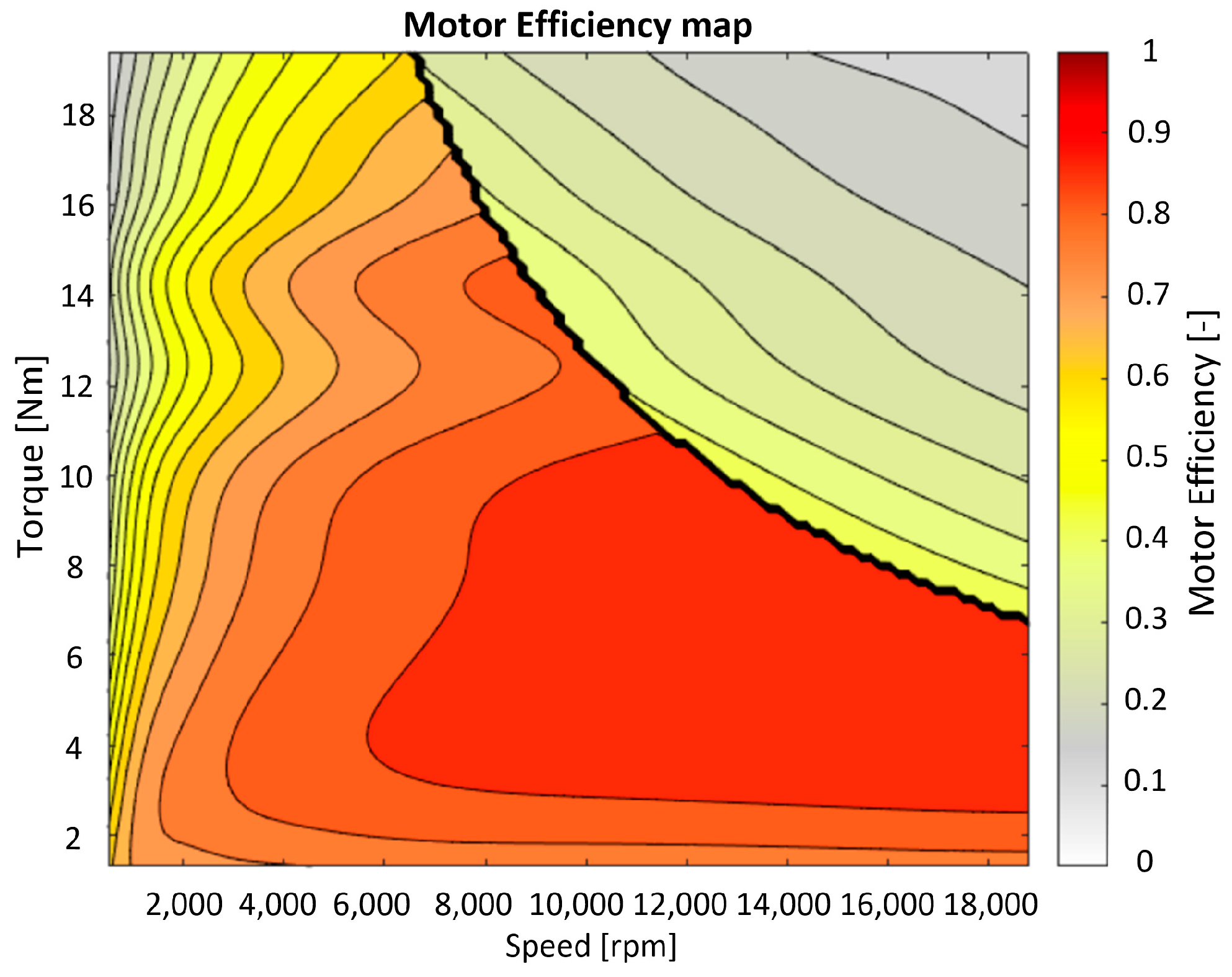
The e-motors’ manufacturer provided an efficiency map with field weakening for different operating conditions in terms of torque and speed. Figure 3 depicts the motor efficiency map for the case of a rear motor when P_max = 40 kW, and the maximum torque was $T_{max}^R$ = 21 Nm. The torque–speed–efficiency map presented in Figure 3 was used to obtain the energy power consumption from the batteries based on the required mechanical power. The motor manufacturer provided this map, and it was corrected to include the motor controller efficiency based on experimental results.

The battery pack comprised LiCO₂ cells, which individually had a nominal voltage of 3.7 V, a charged voltage condition of 4.2 V, and a typical capacity of 7.4 Ah. Assembled in a 140s2p (140 series and 2 parallel) configuration, the battery pack provided a maximum voltage of 588 V and a total theoretical energy capacity of 7.67 kWh. While the theoretical battery capacity was 7.67 kWh, the limiting value at which the vehicle can run was lower. Many factors decreased the available capacity, such as a continuous 600 W low-voltage supply for various systems.

Table 1. Deduction of total available battery pack capacity.

Theoretical capacity	7666 Wh
Low-voltage supply $(~$35 min)	350 Wh
Battery pack losses (3%)	230 Wh
Deviation losses (10%)	767 Wh
Available capacity	6319 Wh

lists the calculations one can perform to better estimate the energy that the fully charged battery pack can deploy.

The knowledge of the available capacity is critical for the optimization process because a small deviation can cause the energy to be drained before the track is complete. Therefore, data from previous endurance runs helped confirm this value, as shown in

Table 2. Maximum capacity extrapolation from endurance data.

Endurance Results	FSG23	FSS23
Initial SOC	98.6%	98.99%
Final SOC	15.2%	17.73%
Energy consumption	5.324 kWh	5.139 kWh
Available capacity	6.405 kWh	6.324 kWh

. With these results in mind, the maximum energy capacity was considered to be E_max = 6.3 kWh.

Furthermore, the prototype was equipped with a Kvaser Memorator Pro 5xHS (Kvaser, Mölndal, Sweden) data logger, which allowed for the post-processing of sensory data included in the CAN communication line. Using its sensor fusion algorithms, the Xsens MTi-670 GNSS/INS (Movella Inc., Henderson, NV, USA) estimates the position, velocity, acceleration, and orientation. Integrated into the battery pack, the Isabellenhutte IVT-S-300-U3-I-CAN2-12/24 (Isabellenhutte, Dillenburg, Germany) outputs voltage, current, power, and energy measurements in real time.

The prototype also incorporated a dedicated PC to handle data processing and generate torque requests directed to the inverters. This computing unit operates internal modules and communicates via a ROS (Robot Operating System)/CAN (Controller Area Network (CAN) Protocol) protocol.

2.2. Vehicle Dynamic Model

The vehicle model built on Newtonian mechanics was based on the dynamic bicycle, dynamic load transfer, and tire models described in [20], and using the models’ parameters previously obtained in Appendix A from [21]. Its geometry can be visualized in Figure 4. The model predicts the evolution of the vehicle state vector x = [X, Y, ψ, v_x, v_y, r]^T. Here, X and Y refer to the vehicle’s global position coordinates, ψ is the vehicle’s orientation, v_x and v_y correspond to the vehicle’s longitudinal and lateral velocities, respectively, and r is the time derivative of the vehicle’s orientation, also known as the yaw rate. The input vector contains the normalized pedal input, p, and the wheel steering angle, δ, described as u = [p, δ]^T.

The longitudinal propulsion force provided by each of the four electric motors is given by (2), where η_t represents the transmission’s efficiency, GR represents the transmission’s gear ratio, r_w is the wheel’s radius, p ∈ [−1, 1] is a normalized pedal input, and T_max is the programmable maximum torque value at a given motor. Additionally, the instantaneous mechanical power used to calculate energy consumption is given by the sum of all four motors (3), where T_i and ω_i are each motor’s operating torque and angular speed, respectively. On the right side of Equation (3), the wheel’s angular speed is converted into rotations per minute (rpm). Finally, η_pt denotes the powertrain system efficiency:

$$F_M={\eta }_t{\displaystyle \frac{\left(p{T}_{max}\right)GR}{r_w}}$$

(2)

$$P=\sum _{i=1}^4{\displaystyle \frac{T_i{\omega }_i}{{\eta }_{pt}}}=\sum _{i=1}^4{\displaystyle \frac{\pi T_i{n}_i}{30{\eta }_{pt}}}$$

(3)

Furthermore, the grip at each tire, F_T, was estimated through individual static loads, F_zstatic, dynamic load transfers, ∆F_{z(x or y)}, and downforce, F_DF, adding up to a given vertical tire load, F_z, which saturates the traction force if under the previously generated motor force ((4) and (5)). In (4), µ_x is a linear longitudinal tire coefficient and µ_xs is the non-linear slope factor. In (5), l_i is the tire’s axle distance to the center of gravity (CoG), and d_fi is the downforce distribution per axle:

$$F_T={\displaystyle \frac{1}{2}}{F}_z({\mu }_x-{\displaystyle \frac{{\mu }_{xs}1}{2}}{F}_z)$$

(4)

$$F_z^i={\displaystyle \frac{m\frac{l_i}{2}g+\frac{1}{2}\rho C_{L}A{v}_x^2{d}_{fi}}{2}}\pm \mathsf{\Delta }{F}_{zx}\pm \mathsf{\Delta }{F}_{zy}$$

(5)

The dynamic load transfer calculations for the longitudinal, ∆F_zx, and lateral directions, ∆F_zy, are described in (6), where m is the car’s total mass, h_cog is the height of the center of gravity, a_x and a_y are the longitudinal and lateral accelerations, respectively, L is the wheelbase, and l_w is the track dimension of the vehicle:

$$\mathsf{\Delta }{F}_{zx}=m{\displaystyle \frac{a_x{h}_{cog}}{L}}, \mathsf{\Delta }{F}_{zy}=m{\displaystyle \frac{a_y{h}_{cog}}{l_w}}$$

(6)

As such, the total longitudinal traction force of the front axle, denoted by $F_x^F$, is the sum of the longitudinal traction forces of both front tires. The same applies to the total longitudinal traction force of the rear axle, denoted by $F_x^R$. In Equation (7), F_x represents the longitudinal forces applied on the vehicle, modeled by the sum of forces around the vehicle’s CoG, such as the electric motor propulsion, rolling, and aerodynamic forces:

$$F_x=F_x^F\cos \left(\delta \right)+F_x^R-C_{R}mg-{\displaystyle \frac{1}{2}}\rho C_{D}A{v}_x^2$$

(7)

To define F_y, denoting the vehicle’s lateral force, one must employ the tire slip angle, ${\alpha }_i$, definition. This angle is defined as the difference between the wheel’s steering angle, ${\delta }_i$, and the wheel’s direction of travel in (8). With the tire slip angles computed and knowing the vertical loads applied on each tire, a simplified version of the model proposed in [22] was used to calculate the resultant lateral forces applied on each tire using (9). This application entails three coefficients to characterize the tire. Coefficient D represents the maximum value of the lateral force for one tire, C is a shape factor, and B is the stiffness factor of the tire:

$${\alpha }_i={\delta }_i-\arctan \left({\displaystyle \frac{v_y-r{l}_i}{v_x\pm \frac{r{l}_w}{2}}}\right)$$

(8)

$$F_y^i=F_z^{i}D \sin \left(C \mathrm{a}\mathrm{r}\mathrm{c}\mathrm{t}\mathrm{a}\mathrm{n}\left({\rm B}{\alpha }_i\right)\right)$$

(9)

As such, the total lateral traction force at the front axle, denoted by $F_y^F$, is the sum of the lateral traction forces of both front tires. The same applies to the total longitudinal traction force of the rear axle, denoted by $F_x^R$. The vehicle’s total lateral force, F_y, is given by (10). So, the continuous-time state–space equations of the dynamic bicycle model can be consulted in Equation (11):

$$F_y=F_y^F\cos \left(\delta \right)+F_y^R$$

(10)

$$\left[\begin{array}{c}\begin{array}{c}\dot{X}\\ \dot{Y}\\ \dot{\psi }\end{array}\\ \begin{array}{c}\dot{v_X}\\ \dot{v_y}\\ \dot{r}\end{array}\end{array}\right]=\left[\begin{array}{c}\begin{array}{c}{v}_x\cos \left(\psi \right)-v_y\sin \left(\psi \right)\\ v_x\sin \left(\psi \right)+v_y\cos \left(\psi \right)\\ r\end{array}\\ \begin{array}{c}{\displaystyle \frac{1}{m}}\left(F_x-F_y^F\mathrm{s}\mathrm{i}\mathrm{n}(\delta )\right)+v_{y}r\\ {\displaystyle \frac{1}{m}}\left(F_y+F_x^F\mathrm{s}\mathrm{i}\mathrm{n}(\delta )\right)-v_{x}r\\ {\displaystyle \frac{1}{I_z}}\left(\left(F_x^F\sin (\delta )+F_y^F\mathrm{c}\mathrm{o}\mathrm{s}(\delta )\right)l_f-F_y^R{l}_r\right)\end{array}\end{array}\right]$$

(11)

2.3. Track Model

Figure 5 illustrates the official FSG 2023 track layout (clockwise direction) obtained from GPS sensor data. The FSG competition track has a single-lap distance of 1220 m. So, the competition defines the total lap number as 18 laps to complete the endurance event, which is worth roughly 22 km.

In the optimization problem, each track segment is considered a variable to be optimized. As a result, the program divides each lap into different track sectors. Each is characterized by a start coordinate, P_i = (X_i, Y_i), and an end coordinate, P_i+1 = (X_i+1, Y_i+1), two arbitrary points in a two-dimensional Cartesian coordinate system. Derived from the Pythagorean theorem, one calculates the respective sector distance with the Euclidean formula (12). Figure 5 shows the track discretization points in blue dots.

$$S_i=\sqrt{{\left(X_{i+1}-X_i \right)}^2+{\left(Y_{i+1}-Y_i\right)}^2}$$

(12)

To avoid a uniform track discretization, which would lead to a drop in accuracy during curves, we performed the discretization based on the maximum possible velocity at curves, defined by (17), and a sampling time of 150 ms. This resulted in a finer section discretization round the curves. The velocity on each track section was then optimized by the optimization algorithm, with a velocity lower than or equal to (17).

By discretizing the track, the vehicle dynamics must be adapted accordingly. For each step, the longitudinal velocity of the vehicle at the following step can be determined based on the current velocity and the difference in kinetic energy, as shown in (13), where $V_i$ and $V_{i+1}$ are the velocities at two consecutive nodes of the track, i and i + 1, $S_i$ is the sector distance defined in (12), and $F_i$ is the total force applied to the vehicle [23]:

$${\displaystyle \frac{1}{2}}m (V_{i+1}^2-V_i^2)=S_i{F}_i$$

(13)

Assuming that the speed is constant while running through a single track sector, the vehicle’s velocity dynamic is defined by (14). Time t is iteratively incremented by each time interval needed for the car to cross each segment, $\mathsf{\Delta }t$, as shown in (15):

$$V_{i+1}=\sqrt{{\displaystyle \frac{2F_i{S}_i}{m}}+V_i^2}$$

(14)

$$t_{i+1}=t_i+\mathsf{\Delta }{t}_i=t_i+{\displaystyle \frac{S_i}{V_i}}$$

(15)

The vehicle’s lap time, T_team, relates to the last value of t_N, which is the accumulated run time after the total number of track sectors, N. Each segment’s energy is computed by multiplying the instantaneous mechanical power (3) with the sector time, $\mathsf{\Delta }{t}_i$. The sector time is variable along the track and is defined by $S_i/V_i.$ The vehicle’s total consumed energy, E_team, is calculated as (16) by accumulating all N sector values and converting to kWh:

$$E_{team}={\displaystyle \frac{{\sum }_{i=1}^N{P}_i\mathsf{\Delta }{t}_i}{3.6\times {10}^6}}$$

(16)

Physically, the car’s velocity at each sector is limited by its maximum velocity, v_top, or the maximum allowed centripetal force, $v_{max}$. This is expressed in (17), where v_top is the vehicle’s top speed, R is the turn radius, D is a tire coefficient that refers to the maximum lateral force in each tire, and m is the vehicle’s mass. This equation only limits the car’s velocity to avoid sliding during curves. The selection of the braking point is performed by the optimization problem, which optimizes the speed for each track section to maximize the endurance and efficiency scores. The braking performance was carried out by considering a drop in average efficiency of 10% of the electric motors when compared with their motor mode. This was calibrated experimentally, and the comparison between the experimental measured power and the simulation ones will be shown in Section 3.

$$v_{max}=\mathrm{m}\mathrm{i}\mathrm{n}\left(v_{top},\sqrt{R{\displaystyle \frac{4D}{m}}}\right)$$

(17)

Moreover, R can be obtained through an iterative implementation of the Menger curvature [24] formula. Given the Cartesian coordinates of three sequential points (x, y, and z), the curvature, C, and subsequent turn radius, R, were calculated as (18) and (19), where A denotes the area of the triangle spanned by x, y, and z:

$$C={\displaystyle \frac{4A}{\left|x-y\right|\left|y-z\right|\left|z-x\right|}}$$

(18)

$$R={\displaystyle \frac{1}{C}}$$

(19)

Note that when the track’s centerline was straight, the curvature (18) tended to zero and the radius (19) tended to infinity. In this case, the vehicle’s maximum achievable velocity, v_max (17), was its maximum straight-line velocity, v_top. Otherwise, its velocity would be limited by the maximum allowable lateral centripetal force, which depends on the vehicle’s mass and tire parameters. Figure 6 depicts the resultant velocity limit values along one lap of the track.

Lastly, the steering angle, δ, required for the vehicle to follow the track, can be determined using (20), where L and l_w are the vehicle’s wheelbase and track width, respectively:

$$\delta =\mathrm{a}\mathrm{r}\mathrm{c}\mathrm{t}\mathrm{a}\mathrm{n}({\displaystyle \frac{L}{R-0.5l_w}})$$

(20)

Note that the above steering angle obtained from GPS data does not necessarily correspond to the track’s centerline. Instead, it reflects the driver’s chosen racing line, known for being more efficient in terms of speed and energy saving.

2.4. Distance Estimation

To ensure that the energy reference setpoint is accurately aligned with the distance traveled, it is imperative to establish a dependable and precise method for odometry calculation. Given the available sensors and the preliminary results using offline simulations with logged data, the methodology chosen for continuous distance estimation during the endurance run was inertial odometry. This estimates a vehicle’s position based on measurements from inertial sensors, typically accelerometers and gyroscopes.

2.5. Optimization Problem

The ultimate goal of the optimization problem is to solve for the maximum points in the sum of the endurance and efficiency scoring. According to FSG’s rules [15], the score for the endurance event is calculated using (21), with 25 points for finishing, and a maximum of 225 points attributed to how fast the car finishes the event, normalized to the fastest car, where T_team is the team’s corrected elapsed time, and T_max is 1.333 times the corrected elapsed time of the fastest vehicle:

$$EN{D}_{score}=25+225\left({\displaystyle \frac{\frac{T_{max}}{T_{team}}-1}{0.333}}\right)$$

(21)

Moreover, the efficiency score is calculated using (22), where a maximum of 75 points is awarded to a team depending on its efficiency factor in comparison to other teams, where EF_min is the lowest (best) efficiency factor of all teams, EF_max is defined as 1.5EF_min, and EF_team is the team’s efficiency factor, given by Equation (23), where T is the uncorrected elapsed driving time, and E is the energy used:

$$EF{F}_{score}=75\left({\displaystyle \frac{E{F}_{max}-E{F}_{team}}{E{F}_{max}-E{F}_{min}}}\right)$$

(22)

$$EF=T^2·E$$

(23)

The results from the most recent competition, FSG23, published in [17], are listed in

Table 3. Resulting formula values from FSG 2023.

FSG2023	Value
Tmax	1.333 × 1396.84 = 1862 s
EFmin	$4.931\times 1490.52=10.955\times {10}^6 \mathrm{kWh}·{\mathrm{s}}^2$
EFmax	$1.5\times 10.955\times {10}^6=16.432\times {10}^6 \mathrm{kWh}·{\mathrm{s}}^2$

.

To maximize the score, considering the vehicle’s powertrain limitations to finish the event plus physical constraints, the cost function prioritizes point scoring according to (21) and (22), aiming to strike a balance between lap-time performance and energy consumption. The optimization problem is defined as follows (24), where the cost function is minimized concerning the pedal’s input state, u = p, and λ_i are soft constraints’ weights, allowing control over two crucial soft constraints:

$$\begin{gathered} \mathrm{m}\mathrm{i}\mathrm{n}\left(-\left(EN{D}_{SCORE}+EF{F}_{SCORE}\right)+{\lambda }_1{V}_{pen}+{\lambda }_2{E}_{pen}\right) \\ \mathrm{s}.\mathrm{t}. {\mathrm{A}}_{\mathrm{i}\mathrm{n}\mathrm{e}\mathrm{q}}u\le b_{ineq} \end{gathered}$$

(24)

At each sector, the vehicle cannot exceed a maximum velocity, which is either limited by the maximum allowed centripetal force or the vehicle’s maximum velocity (25). Also, the vehicle must not exceed the maximum energy capacity of the battery pack, as, in the real event, it would result in a DNF (Did Not Finish), scoring zero points (26):

$$V_{pen}=\sum _{i=1}^N\mathrm{m}\mathrm{a}\mathrm{x}(0, V_i-v_{{\mathrm{m}\mathrm{a}\mathrm{x}}_i})$$

(25)

$$E_{pen}=\mathrm{m}\mathrm{a}\mathrm{x}(0, E_{team}-E_{max})$$

(26)

Regarding the control input, u = p, there are two inequality constraints, which, algebraically written, are given by the following matrices:

$$A_{ineq}=\left[\begin{array}{cc}-1& 0\\ 1& 0\end{array}\right], b_{ineq}=\left[\begin{array}{c}1\\ 1\end{array}\right]$$

(27)

A simulator was developed in MATLAB 2023b to run the optimization environment (Figure 7). It starts by initializing an app interface that asks the user to input the track layout, vehicle’s physical and powertrain parameters, and optimization parameters. After discretizing the track environment, the program simulates multiple iterations of the endurance event using the appropriate vehicle model, while optimizing the control vector with the cost function (24) to maximize the scores in both endurance and efficiency events. For this purpose, the MATLAB optimizing function fmincon is used to find the optimal solution given the constraints or a limit of iterations. After reaching the optimal solution, an output file containing the optimized energy reference line in function of the distance is generated.

2.6. Controller Implementation

2.6.1. Endurance Energy Manager

The system takes an optimal energy reference line in function of distance as its input and continually adapts the vehicle’s maximum power constraint, denoted as P_max. Given the endurance distance status, this adjustment depends on whether the current energy level exceeds or falls short of the expected energy level. An error (28) is computed between the current energy level and the referenced setpoint. This depends on continuous distance estimation, d, along the endurance event:

$$E_{error}=E_{ref}\left(d\right)-E_{real}$$

(28)

Then, the new vehicle’s maximum power (29), P_max, is computed using a simple PI controller on the error resultant from (28) to compute the power limit adjustment, which is then added to/subtracted from the initial power-limiting value, P_init. In (29), K_p and K_i are controller gains, proportional and integral, respectively. These gains are used to tune the aggressiveness of the power limit adjustments:

$$P_{max}=P_{init}+(K_p{E}_{error}+K_i{\int }_0^t{E}_{error}dt)$$

(29)

2.6.2. Distance Estimation Methodology

The results of running offline simulations with this measure on different endurance log samples are shown in

Table 4. Different odometry methodologies’ results.

Log Run	Inertial Odometry	Actual Distance
Alverca	21,250 m	21,378 m
FSG23	22,070 m	21,924 m
FSS23	20,760 m	20,900 m

. As can be seen, the differences between the estimated distances and the actual ones were very close, with a deviation of less than 0.7%.

However precise, the methodology above remains susceptible to error accumulation throughout the lengthy endurance event. To address this challenge, a new system was introduced. The position validator operates by continuously monitoring distance estimates derived from inertial odometry, aligning them with expected positions on the track layout. It then validates the distance estimate by performing real-time cross-validation with the GPS outputs. The algorithm compares the expected track position with the actual GPS-derived position, computing the Euclidean distance (12) and checking if it falls within an acceptable threshold. The threshold is expressed as a maximum radius around the expected point, R_max. In cases where the distance discrepancy exceeds this threshold (∆d > R_max), indicating error accumulation over what is deemed acceptable, the system dynamically corrects the distance using GPS data and adjusts for the elapsed number of laps.

Using logged data from the most recent endurance event (FSG23), with the maximum acceptable discrepancy defined at R_max = 5 m, the position validator eliminated the accumulated residual error of the inertial odometry worth over 140 m, as seen in Figure 8.

2.6.3. Pipeline Implementation

The controller now implemented relates to the Endurance Energy Manager, who dynamically adjusts the vehicle’s power limitation to ensure that the vehicle closely adheres to the pre-established optimal energy reference line, Figure 9. Similar to the rest of the pipeline, the module was programmed in its own SIMULINK 2023b model, incorporating MATLAB functions. After being tested offline, the code was generated in C++ using the SIMULINK Coder built-in feature, and the target file was set appropriately. A working frequency of 10 Hz was chosen for the Endurance Energy Manager module. Finally, the C++-generated code was implemented on the team’s ROS/CAN communication pipeline. New signals were added to the CAN line, and the appropriate signal/module connections were made in the ROS communication pipeline. The module’s inputs are as follows:

• IMU: 3 × 1 vector containing IMU readings (v_x, v_y, and ψ).
• GPS: 2 × 1 vector containing GPS readings (latitude and longitude).
• isa_energy: accumulated energy value, in Wh.
• EM_enable: turns the controller module “on/off”.
• max_pwr: limits total power as a safety measure, in W.
• init_PL: algorithm’s initial power-limiting value, in W.
• EM_kp: controller’s proportional gain.
• EM_ki: controller’s integral gain.
• d_prev: discretely accumulated distance value, in m.

The outputs are as follows:

• EM_pwrlimit: Energy Manager algorithm P_max computation, in W.
• pwr_limit: sent to the power limiter.
• $pw{r}_{limit}=\left\{\begin{array}{c}E{M}_{pwrlimit}, \mathrm{i}\mathrm{f} E{M}_{enable}=1\\ {max}_{pwr}, \mathrm{o}\mathrm{t}\mathrm{h}\mathrm{e}\mathrm{r}\mathrm{w}\mathrm{i}\mathrm{s}\mathrm{e}\end{array}\right.$
• d: accumulated distance run by the vehicle.
• e_ref: current energy reference setpoint, E_ref(d).

3. Results

3.1. Model Mismatch

Prior to the optimization, it was important to test the developed models and compare the outputs to real measurements, using the same inputs to try and validate the outputs. Thus, the models were developed in SIMULINK and fed with real logged driving data regarding the fastest FSG endurance event lap as input.

Table 5. Velocity and energy mean-squared error model mismatch.

Mean-Squared Error	Velocity (m/s)	Energy (Wh)
Point mass vehicle model	2.96	33.92
Dynamic bicycle model	0.48	2.26

shows the mean-squared error results for velocity and energy outputs obtained by sensors compared to their reference.

In light of these results, due to its closer representation of the real prototype in racing conditions, the chosen model was the dynamic bicycle model. Additionally, the optimization process entailed multiple iterations, each characterized by its runtime, influenced by model complexity and the number of variables (sectors). Due to extended runtimes in SIMULINK for each iteration, it was necessary to discretize the process in MATLAB. This was executed, and

Table 6. Velocity and energy mean-squared error simulation mismatch.

Mean-Squared Error	Velocity (m/s)	Energy (Wh)
Continuous lap simulation	0.48	2.26
Discretized lap simulation	0.57	3.47

lists the results.

To observe where the model was lacking the most, Figure 10 represents a velocity mismatch percentage factor along the track layout, given by V/V_real. This computes values over 1 when the model estimates the vehicle driving faster than in reality, and values under 1 when estimating a lower velocity. The same can be seen in Figure 11, where the comparison between the real measured power and the continuous and discrete simulation models’ results are presented, for a single lap.

Predominantly, there was a slight overestimation (yellow) of the vehicle’s velocity in straights and an underestimation (blue) in most tight corners. The effectiveness of the multivariable optimization process was significantly impacted by the number of variables represented by track partitions in this context. This influence extended to both model accuracy and computational speed.

To evaluate the influence of the number of track sectors on the velocity mismatch and computational time, a study was conducted by changing the number of track sectors and comparing the final results with the continuous model. Figure 12 shows the evolution of the velocity mean-squared error and the computational time as a function of the number of track sectors. Beyond 3000 lap sectors, there was marginal improvement in terms of model accuracy, while the single iteration time steadily increased linearly. This had substantial implications for the optimization time, particularly when the process involved computing thousands of iterations to identify the optimal solution. Thus, the number of track sectors was defined as 3000.

3.2. Optimization Results

In the endurance event, the focus was on lap time optimization and energy consumption. The balance was modeled in the cost function (24). The objective was to achieve the highest joint score while ensuring the car completed the 22 km distance within its maximum energy capacity and physical limitations. Running the optimization of the FST12 prototype around an 18-lap endurance event on the official 2023 FSG track layout (see Figure 5), the resulting velocity profile along time is shown in Figure 13. Additionally, it was compared to the maximum velocity in each track section, as defined in Equation (17), and with the real track data obtained from the competition in 2023 (FST12, FSG23) without the energy optimization algorithm. Figure 14 shows the resulting power deployment along the lap.

As one can observe, the optimization saw the vehicle matching maximum corner speeds for lap time reduction and managed energy in the two main straights (especially), easing off the throttle and even regenerating slightly (see Figure 14).

In summary, the optimized profile of the FST12 completed the simulated FSG endurance event with a total elapsed time of 1520 s, consuming a total energy of 5.985 kWh (out of 6.3 kWh), showing that it is not optimal to consume all available energy for maximum points. As a result, the average lap time was 84.44 s, with an energy consumption of 0.333 kWh per lap, which would result in 177 points and an additional 35.7 points for efficiency, bringing the total to 212.7 points out of 325, as illustrated in Figure 15. Also, this figure shows the real points obtained by the FST team in the competitions of 2022 (FST11, FSG22) and 2023 (FST12, FSG23, data in Figure 13) without energy optimization. This optimization process can achieve a high increase without changing the vehicle’s performance and structure.

3.3. On-Track Results

For the test run, the routine expected in competitions was performed on a real track in Alverca, Portugal. The practical plan for using the system involved first optimizing the endurance profile based on the track data gathered during the Autocross event (held a day before the endurance event). Afterward, the optimized plan was uploaded to the car’s control unit, and the energy monitoring system was enabled to run throughout the event. Given the absence of other teams for competitive benchmarks on the final test run day and the inability to fully recreate one of the already existing layouts, a better team was assumed to be 5% faster and 15% more efficient than a representative Autocross lap set by the FST12 around the track in question. So, the driver performed a total of 4 laps, and the average lap time was 72 s, with an average energy consumption of 0.26 kWh per lap. The chosen track had a lap distance of 884 m, adhering to FS layout regulations [17], and the run programmed in this test consisted of 22 laps around the circuit.

After the initial Autocross runs, the battery pack was charged back up to nearly 95%. In the meantime, the track data were extracted, and the offline optimization was performed. The result for the velocity profile around the layout can be consulted in Figure 16.

Overall, the FST12 completed the simulated event with a total elapsed time of 1522.1 s, consuming a total energy of 5.355 kWh. The average lap time was 70.55 s, with an energy consumption of 0.243 kWh per lap, resulting in 222.6 points for the endurance event and an additional 49.2 points for efficiency, bringing the total to 271.8 points out of 325. Having concluded the optimization, the resulting energy plan was uploaded to the car’s control unit’s energy management system and the endurance run began.

In reality, the FST12 completed the full Alverca endurance run in 1574.6 s, consuming a total energy of 5.383 kWh. An onboard video of one of the endurance laps can be found in https://youtu.be/jT0GfjM5nTc?si=CtbzNcQ4KxO0plLC (accessed on 12 December 2024). Compared to the optimization-based simulation, the results are presented in

Table 7. Final run results in comparison to the optimization.

Results	Time (s)	Energy (kWh)	Points
Optimization	1522.1	5.355	271.8
Final run	1574.6	5.383	253.1
Deviation	1.4%	0.5%	6.8%

, with each respective deviation. Furthermore, the power limit adjustments over time compared to the real power output are shown in Figure 17, and one can see that over the run, it allowed for proper adherence to the energy reference line, as shown in Figure 18. The run’s total distance estimation resulted in 19,894 m, which deviated from the expected measured 19,448 m (22 laps of 884 m each) by 2%. The deviation between the simulation and experimental results may originate from several sources: deviation of the model’s parameters, discretization of the models, and the errors associated with the distance estimation methodology to determine the real position of the car throughout the track. However, it should be noted that the discretization of the model and the calibration of the tire model should have a higher impact for this deviation. These assumptions were required to allow for a good trade-off between accuracy and computational time, which is required for the score optimization problem.

It is important to acknowledge that while the achievements of a well-optimized offline simulation provide a strong foundation, they may not entirely capture the complexities of an actual endurance event. In the dynamic context of an endurance event with multiple participating cars, various factors come into play that can significantly impact the optimization process. These include unforeseen events, such as yellow flags resulting from vehicle breakdowns or blue flags to inform slower-moving cars that they must temporarily pull over to a designated area to allow a faster car to overtake, both of which request unaccounted-for driver responses. Such occurrences disrupt the anticipated optimization outcomes.

Additionally, the driver change halfway through the endurance event introduces additional challenges. Penalties are not accounted for in the optimization yet occur occasionally and have the potential to push the vehicle beyond the boundaries of the efficiency scoring window. Consequently, there may come a point where prioritizing pure speed over efficiency becomes more advantageous for the point-scoring tally.

These aspects highlight the need for future research to delve deeper into the intricacies of real-world scenarios and refine optimization strategies to adapt to the event-evolving dynamics of Formula Student endurance events.

4. Conclusions

This work proposed a methodology to optimize the energy use of competitive electric vehicles and implement it in a real case study. The Formula Student competition was used as an implementation case to evaluate this methodology.

The methodology first required complete vehicle characterization, involving the development of models grounded in the principles of vehicle dynamics. These models were validated, utilizing a data-driven approach to define powertrain efficiency and the battery pack’s capacity. The employed vehicle model provided a mismatch to reality of under 5% for both velocity and energy model outputs during a full racing lap around the FSG track.

An optimization-based simulation framework was established to simulate endurance runs, with the flexibility to configure key parameters, such as powertrain characteristics and the starting conditions of the run. The overall goal was to maximize the points scored according to the regulations based on the driving profile and subsequent optimal energy deployment over distance. Following this, we developed an energy management system capable of employing a low-level controller that periodically dynamically adjusts the prototype’s maximum power limitation along the run. This involved continuously monitoring the real-time error, calculated as the difference between the reference and actual energy consumed, as measured by an appropriate sensor.

The proposed methodology was validated in a real endurance run at a test track. The developed energy management control system was implemented, guided by a previously simulated optimal reference. This reference was tailored to maximize endurance and efficiency points in the new track layout relative to a normalized best score. In summary, compared to the optimal simulation, a 20 km endurance run had a total time mismatch of 1.4% and a total energy mismatch of 0.5%, leading to a discrepancy of 6.8% from the simulated and actual points prospect.

This approach, merging theoretical modeling with a data-driven perspective and testing the prototype, proved to be an efficient energy optimization method for electric vehicle applications, particularly the Formula Student endurance competitions.