Sliding Mode Control and Immersion & Invariance Observer for Grid-Tied Inverters in Photovoltaic Applications: Continuous Operation for Power Quality Enhancement

Abstract

This work proposes a model-based control scheme using a sliding mode controller (SMC) and an immersion and invariant (I&I) observer. The objective of the proposed control scheme is to be applied to a three-phase grid-tied inverter, which could operate as a shunt active power filter when the photovoltaic array is not generating power (night-time operation). The grid-tied inverter always remains operational, ensuring continuous support of the power quality improvement, as well as current harmonic compensation due to nonlinear loads and power factor correction. An external control loop is included to keep the voltage of the DC-link capacitor regulated. As can be explained in detail along with the work, a battery stack is avoided in this proposed research. Thus, a decision stage is added to the control scheme to select the night or day operation. Simulation results are carried out using Altair-PSIM© to demonstrate the effectiveness of the proposed control scheme in several scenarios.

1. Introduction

Solar energy is one of the most widely embraced alternative energy sources globally [1]. Thanks to technological advancements and cost reductions, rooftop photovoltaic systems have experienced significant growth in recent years. With the increasing adoption of distributed renewable energy, the number of inverters connected to the grid has risen. These inverters are an important power stage and are crucial to enabling photovoltaic panels to inject current into the grid. However, their nonlinear characteristics introduce harmonics to the grid, causing negative effects on grid operations and connected devices [2].

The repercussions of harmonic pollution range from diminished power generation efficiency to potential damage to sensitive equipment, such as computers, due to distorted waveforms caused by harmonics. On the one hand, a reduction in efficiency is presented; on the other hand, it also requires suppliers to provide additional power to compensate for distortion losses [3]. In [4], standards are outlined, detailing requirements and recommended practices for interconnection with distributed generation to the grid to address harmonic pollution. The Electric Research Power Institute has also released photovoltaic grid integration protocols that include methods for harmonic compensation and control modes [5].

Inverter hardware is frequently idle during periods of diminished solar intensity when the photovoltaic (PV) system does not generate sufficient voltage to inject power into the grid. During such periods, there is an opportunity to take advantage of the inverter by re-purposing its hardware as an active power filter (APF). Active power filters (APFs) act as a harmonic source to mitigate harmonic effects on the electrical grid, as discussed in [6,7].

Several studies have addressed power quality issues by integrating renewable energy conversion systems into the grid, avoiding the need for an additional power compensation system. In [8], the associated challenges to the integration of renewable resources into the electrical grid, including requirements for power quality, are thoroughly detailed. Another study, presented in [9], offers information that could help industrial researchers improve the quality of the power of electrical grids by utilizing renewable energy.

The work mentioned in [9] involves controlling the PV inverter to maintain a synchronized sinusoidal current in the grid that is in phase with the AC-mains. This approach achieves a unitary power factor and regulates the DC-link voltage. Additionally, ref. [10] employs an inverter as an APF to eliminate total harmonic distortion (THD) generated by nonlinear loads on end users in various operational scenarios. In all cases, the reduction in THD serves as a clear indicator of the improvement in the quality of the power supply.

As mentioned above and in alignment with [11], during daylight hours when there is ample sunlight, the PV inverter channels the active power produced by the photovoltaic cells into the grid. Consequently, the functions assigned to this inverter include harmonic reduction, reactive power compensation, and inclusive phase balancing, as described in [12]. Regardless of the inverter’s technology, the choice of a control scheme is crucial for its proper functionality [12].

As discussed in [13], various control techniques have been reported; the most used are proportional–integral (PI), repetitive, hysteresis, linear quadratic regulator (LQR), and fuzzy logic control (FLC). Additional work explores less commonly cited techniques such as passivity-based control (PBC) [14] and sliding mode control (SMC) [15]. Scientists in the former Soviet Union mainly studied the SMC technique. The SMC scheme is a well-established discontinuous feedback control method extensively explored in the literature [16]. This technique is especially well-suited for regulating switched-controlled systems, including power electronics devices. Hence, studies such as that presented in [17] strongly recommend applying this controller to power inverters.

In [18,19], a seven-level inverter is controlled using SMC, demonstrating high dynamic performance and robustness against disturbances and parameter mismatches. SMC is also applied to a single-phase PV grid-connected voltage source inverter (VSI) with an L filter in [20], revealing a quick response time of less than one grid frequency cycle and no overshoot. Another instance is reported in [21], focusing on a sliding mode controller for single-phase quasi-Z source inverters, where experiments show fast dynamic response, robustness, and simplicity in implementation. The feasibility and performance of the proposed control approach are further validated through experimental results under both linear and nonlinear load conditions. Furthermore, [22] details the application of SMC for a voltage source inverter under distorted grid voltage. In this reference, simulation and experimental results are dedicated to showing the reduction of total harmonic distortion (THD) in currents, which is consistent with the IEEE standard for harmonic control in electrical power systems.

This paper examines the effectiveness of the control strategy suggested when implemented in a PV grid-tied inverter, which operates continuously as an APF, day and night. This involves reactive power compensation and minimizing total harmonic distortion (THD). The subsequent section describes the grid-tied inverter and presents its mathematical model. Additionally, the proposed control system is thoroughly outlined. The system’s performance is assessed through simulation tests, and concluding remarks are addressed in the final sections.

2. Power System Description

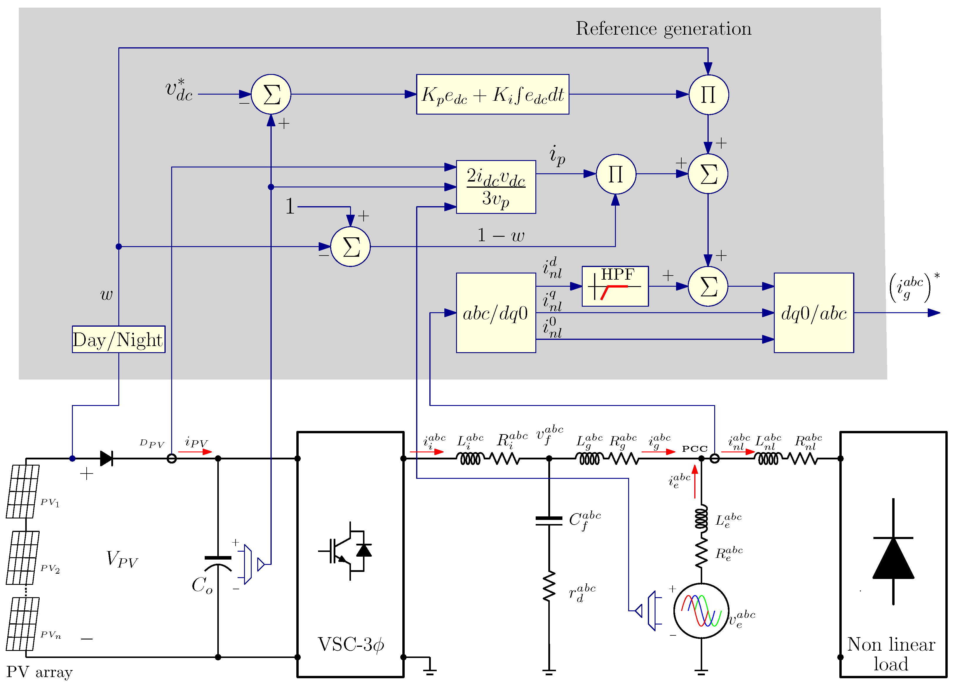
The schematic representation of a three-phase grid-tied inverter that supplies power to a set of loads connected to the point of common coupling (PCC) under investigation is illustrated in Figure 1. This configuration closely resembles the one depicted in [23], in which the dynamics of the circuit are explained, treating it as a three-phase balanced system, as outlined below:

$$\begin{array}{c}{\displaystyle \frac{d{v}_f^{abc}}{dt}}={\displaystyle \frac{i_i^{abc}-i_g^{abc}}{C_f^{abc}}}\\ {\displaystyle \frac{d{i}_g^{abc}}{dt}}={\displaystyle \frac{v_e^{abc}-v_f^{abc}}{L_g^{abc}}}\\ {\displaystyle \frac{d{i}_i^{abc}}{dt}}={\displaystyle \frac{v_f^{abc}}{L_i^{abc}}}+{\displaystyle \frac{v_{CD}}{3L_i^{abc}}}\Gamma u\end{array}$$

(1)

with:

$i_i^{abc}={\left[i_i^a{i}_i^b{i}_i^c\right]}^T$ are the inverter side inductor currents;

$i_g^{abc}={\left[i_g^a{i}_g^b{i}_g^c\right]}^T$ are the grid side inductor currents;

$v_e^{abc}={\left[v_e^a{v}_e^b{v}_e^c\right]}^T$ are the grid voltages;

$u^{abc}={\left[u^a{u}^b{u}^c\right]}^T$ are the control signals;

$v_f^{abc}={\left[v_f^a{v}_f^b{v}_f^c\right]}^T$ are the LCL capacitor voltages;

$\Gamma =\left[\begin{array}{ccc}-2& 1& 1\\ 1& -2& 1\\ 1& 1& -2\end{array}\right]$;

$C_f^{abc}=C_{fa}=C_{fb}=C_{fc}$ are the LCL filter capacitors;

$L_g^{abc}=L_{ga}=L_{gb}=L_{gc}$ are the grid side LCL filter inductors;

$L_i^{abc}=L_{ia}=L_{ib}=L_{ic}$ are the inverter side LCL filter inductors.

In Figure 1, it is important to note the inclusion of a diode ($D_{PV}$) placed between the photovoltaic array and the DC capacitor $C_o$. In this context, the power diode acts as an isolator to prevent the photovoltaic array from acting as a load on the system when the power converter works as an APF. Consequently, the mathematical model differs from the one previously presented in [23] by the authors due to the voltage decoupling between the DC capacitor and the PV array. This decoupling increases the overall order of the system, as the DC input voltage of the inverter $v_{DC}$ is now equivalent to the voltage of the capacitor $C_o$ rather than the voltage of the photovoltaic array. With this consideration, the DC input voltage of the inverter $v_{DC}$ can be defined as

$$\begin{array}{c}{\displaystyle \frac{d{v}_{DC}}{dt}}={\displaystyle \frac{i_i^a{u}^a+i_i^b{u}^b+i_i^c{u}^c}{C_o}}w\end{array}$$

(2)

where w is the flag that indicates the operation mode of the system as follows:

$$w=\left\{\begin{array}{cc}\begin{array}{c}0\\ 1\end{array}\hfill & \begin{array}{c}\mathrm{during}\mathrm{power}\mathrm{generation}.\\ \mathrm{without}\mathrm{power}\mathrm{generation}.\end{array}\hfill \end{array}\right.$$

(3)

Finally, the complete representation of the three-phase grid-tied inverter that supplies power to a set of loads connected to the PCC is formulated as follows:

$$\begin{array}{c}{\displaystyle \frac{d{v}_f^{abc}}{dt}}={\displaystyle \frac{i_i^{abc}-i_g^{abc}}{C_f^{abc}}}\\ {\displaystyle \frac{d{i}_g^{abc}}{dt}}={\displaystyle \frac{v_e^{abc}-v_f^{abc}}{L_g^{abc}}}\\ {\displaystyle \frac{d{i}_i^{abc}}{dt}}={\displaystyle \frac{v_f^{abc}}{L_i^{abc}}}+{\displaystyle \frac{v_{CD}}{3L_i^{abc}}}\Gamma u\\ {\displaystyle \frac{d{v}_{DC}}{dt}}={\displaystyle \frac{{\left(i_i^{abc}\right)}^T{u}^{abc}w}{C_o}}\end{array}$$

(4)

3. Control Description

The proposed control strategy is designed to enable a PV inverter to act as an active power filter. To achieve this, several tasks need to be performed:

• Inject active power during power generation;
• Regulate the DC voltage during non-generation periods;
• Improve the low power factor caused by inductive loads;
• Minimize the harmonic distortion introduced by nonlinear loads.

The control scheme proposed in this research consists of three main stages: (1) the control scheme, (2) the estimation stage, and (3) the reference calculation stage. Each of these stages is described in detail in the following subsections.

3.1. Control Stage

Given the nonlinear nature of the system, a discontinuous sliding mode controller was selected. This controller operates on a sliding surface defined as [24,25]

$$\sigma =L_i^{abc}\left(i_i^{abc}-{\left(i_i^{abc}\right)}^{*}\right)=0$$

(5)

where ${\left(i_i^{abc}\right)}^{*}={\left[{\left(i_i^a\right)}^{*}{\left(i_i^b\right)}^{*}{\left(i_i^c\right)}^{*}\right]}^T$ represents the reference current vector for the inverter side inductor. The time derivative of the sliding surface is given by

$${\displaystyle \frac{d\sigma }{dt}}=L_i^{abc}\left({\displaystyle \frac{d{i}_i^{abc}}{dt}}-{\displaystyle \frac{d{\left(i_i^{abc}\right)}^{*}}{dt}}\right)=0$$

(6)

The above controller ensures that the system trajectories remain on the sliding surface; however, additional control is required to drive the trajectories toward the surface. This additional control signal is derived from the following candidate Lyapunov function:

$$W\left(\sigma \right)={\displaystyle \frac{1}{2}}{\sigma }^2\ge 0$$

(7)

with a time derivative given by

$${\displaystyle \frac{dW\left(\sigma \right)}{dt}}={\sigma }^T{\displaystyle \frac{d\sigma }{dt}}.$$

(8)

The attractiveness of the sliding surface is guaranteed when ${\displaystyle \frac{dW\left(\sigma \right)}{dt}}\le 0$. Therefore, it is necessary that

$${\displaystyle \frac{dW\left(\sigma \right)}{dt}}=-\kappa \left|\begin{array}{c}\sigma \end{array}\right|.$$

(9)

where $\kappa$ is a positive constant.

By matching the derivatives (8) and (9) we obtain

$${\sigma }^T{\displaystyle \frac{d\sigma }{dt}}=-\kappa \left|\begin{array}{c}\sigma \end{array}\right|.$$

(10)

By substituting Equations (5) and (6) into (10) we have

$$\begin{array}{c}{\left(L_i^{abc}\right)}^2{\left(i_i^{abc}-{\left(i_i^{abc}\right)}^{*}\right)}^T\left({\displaystyle \frac{d{i}_i^{abc}}{dt}}-{\displaystyle \frac{d{\left(i_i^{abc}\right)}^{*}}{dt}}\right)\hfill \\ =-\kappa \left|\begin{array}{c}{L}_i^{abc}\left(i_i^{abc}-{\left(i_i^{abc}\right)}^{*}\right)\end{array}\right|.\hfill \end{array}$$

(11)

Applying the definition of the absolute value ($\left|x\right|=x\mathrm{sign}\left(x\right)$) in Equation (11), we obtain the following:

$$\begin{array}{c}{L}_i^{abc}\left({\displaystyle \frac{d{i}_i^{abc}}{dt}}-{\displaystyle \frac{d{\left(i_i^{abc}\right)}^{*}}{dt}}\right)=-\kappa \mathrm{sign}\left(i_i^{abc}-{\left(i_i^{abc}\right)}^{*}\right).\hfill \end{array}$$

(12)

Now, by taking ${\displaystyle \frac{d{i}_i}{dt}}$ from Equation (4) and substituting it into Equation (12), we obtain

$$v_f^{abc}+{\displaystyle \frac{v_{DC}}{3}}\Gamma u^{abc}-L_i^{abc}{\displaystyle \frac{d{\left(i_i^{abc}\right)}^{*}}{dt}}=-\kappa \mathrm{sign}\left(i_i^{abc}-{\left(i_i^{abc}\right)}^{*}\right).$$

(13)

The control law that drives the system toward the sliding surface is given by

$$u^{abc}=3{\Gamma }^{-1}{\displaystyle \frac{-v_f^{abc}+L_i^{abc}\frac{d{\left(i_i^{abc}\right)}^{*}}{dt}-\kappa \mathrm{sign}\left(i_i^{abc}-{\left(i_i^{abc}\right)}^{*}\right)}{v_{DC}}}.$$

(14)

This control strategy guarantees stability in the vicinity of the sliding surface defined by $\sigma =0$.

3.2. Inductor Current Estimator

In power converter control, conventional methods typically rely on measured signals, such as current and voltage, from components such as inductors, capacitors, diodes, and others. However, with the advent of microcontrollers, DSPs, and other digital platforms, it is now straightforward to implement observers that estimate electrical variables without compromising accuracy, thereby enhancing reliability. This approach is particularly advantageous, as physical sensors can introduce noise into the measurements. Furthermore, an advantage of using observers is the reduction in the cost of the control system by eliminating the need for physical sensors [26].

The proposed control strategy employs an immersion and invariance (I&I)-based observer to estimate the inductor currents from the voltage measured across the LCL filter capacitors. The selection of the I&I technique is supported by its proven robustness and fast convergence rate [27].

The design of the observer begins by defining the estimation error as

$$z=x_i-{\widehat{x}}_i+C_f^{abc}\chi \left(v_f^{abc}\right),$$

(15)

where $x_i={\left[\begin{array}{cccccc}{i}_g^a& i_g^b& i_g^c& i_i^a& i_i^b& i_i^c\end{array}\right]}^T$, ${\widehat{x}}_i={\left[\begin{array}{cccccc}{\widehat{i}}_g^a& {\widehat{i}}_g^b& {\widehat{i}}_g^c& {\widehat{i}}_i^a& {\widehat{i}}_i^b& {\widehat{i}}_i^c\end{array}\right]}^T$ represent the estimated inductor currents, and $\chi$ is a function of $v_f^{abc}$ designed to drive the estimation error to zero.

The dynamics of the estimation error are driven to converge to zero by taking the time derivative of Equation (15) as follows:

$${\displaystyle \frac{dz}{dt}}={\displaystyle \frac{d{x}_i}{dt}}-{\displaystyle \frac{d{\widehat{x}}_i}{dt}}+C_f^{abc}{\displaystyle \frac{\partial \chi }{\partial v_f^{abc}}}{\displaystyle \frac{d{v}_f^{abc}}{dt}}.$$

(16)

In this case, it is proposed to use the following:

$$L{\displaystyle \frac{dz}{dt}}=L{\displaystyle \frac{d{x}_i}{dt}}-L{\displaystyle \frac{d{\widehat{x}}_i}{dt}}+L{C}_f^{abc}{\displaystyle \frac{\partial \chi }{\partial v_f^{abc}}}{\displaystyle \frac{d{v}_f^{abc}}{dt}},$$

(17)

where $L=\left[\begin{array}{cc}{L}_g^{abc}M& N\\ N& L_i^{abc}M\end{array}\right]$, with $M=I_3$ and $N=0_{3,3}$.

Now, by substituting the time derivatives into the observation error dynamics in Equation (17), we obtain

$$\begin{array}{cc}\hfill L{\displaystyle \frac{dz}{dt}}=& \left[\begin{array}{c}{v}_e^{abc}-v_f^{abc}\\ v_f^{abc}+{\displaystyle \frac{\Gamma u^{abc}{v}_{CD}}{3}}\end{array}\right]-L{\displaystyle \frac{d{\widehat{x}}_i}{dt}}\hfill \\ \hfill & +L{\displaystyle \frac{\partial \chi }{\partial v_f^{abc}}}\left[\begin{array}{cc}M& -M\end{array}\right]x_i.\hfill \end{array}$$

(18)

To eliminate the measured currents from the error dynamics equation, $x_i$ is extracted from the definition of the estimation error in Equation (15) and substituted into Equation (18). The observer error dynamics is then formulated as follows:

$$\begin{array}{c}L{\displaystyle \frac{dz}{dt}}=\left[\begin{array}{c}{v}_e^{abc}-v_f^{abc}\\ v_f^{abc}+{\displaystyle \frac{\Gamma u^{abc}{v}_{CD}}{3}}\end{array}\right]-L{\displaystyle \frac{d{\widehat{x}}_i}{dt}}\\ +L{\displaystyle \frac{\partial \chi }{\partial v_f^{abc}}}\left[\begin{array}{cc}M& -M\end{array}\right]\left[z+{\widehat{x}}_i-C_f^{abc}\chi \left(v_f^{abc}\right)\right].\end{array}$$

(19)

Defining the observer as

$$\begin{array}{c}L{\displaystyle \frac{d{\widehat{x}}_i}{dt}}=\left[\begin{array}{c}{v}_e^{abc}-v_f^{abc}\\ v_f^{abc}+{\displaystyle \frac{\Gamma u^{abc}{v}_{CD}}{3}}\end{array}\right]\\ +L{\displaystyle \frac{\partial \chi }{\partial v_f^{abc}}}\left[\begin{array}{cc}M& -M\end{array}\right]\left[{\widehat{x}}_i-C_f^{abc}\chi \left(v_f^{abc}\right)\right],\end{array}$$

(20)

the observer error dynamics (19) simplifies to

$$L{\displaystyle \frac{dz}{dt}}={\displaystyle \frac{\partial \chi }{\partial v_f}}\left[\begin{array}{cc}M& -M\end{array}\right]\left[z\right];$$

(21)

it is evident that the stability of the observer error dynamics is guaranteed if the matrix ${\displaystyle \frac{\partial \chi }{\partial v_f^{abc}}}\left[\begin{array}{cc}M& -M\end{array}\right]$ is at least semi-definite negative. This condition is satisfied by defining $\chi \left(v_f^{abc}\right)=K\left[\begin{array}{c}-M\\ M\end{array}\right]v_f^{abc}$, with $K>100$.

It should be noted that the definition of $\chi \left(v_f^{abc}\right)$ is not unique.

Finally, the dynamics of the observer error is given by

$$L{\displaystyle \frac{d{\widehat{x}}_i}{dt}}=\left[\begin{array}{c}{v}_e^{abc}-v_f^{abc}\\ v_f^{abc}+{\displaystyle \frac{\Gamma u^{abc}{v}_{CD}}{3}}\end{array}\right]+K\left[\begin{array}{cc}-M& M\\ M& -M\end{array}\right]\left[{\widehat{x}}_i\right].$$

(22)

The following quadratic Lyapunov candidate function is proposed to verify the stability of the whole system:

$$V(\sigma ,z)={\displaystyle \frac{1}{2}}\left[\begin{array}{cc}{\sigma }^T& z^T\end{array}\right]\left[\begin{array}{cc}I& 0\\ 0& L\end{array}\right]\left[\begin{array}{c}\sigma \\ z\end{array}\right]>0\forall \{\sigma ,z\}\ne 0,$$

(23)

where $\sigma$, z, and the matrix L were previously defined in Equations (5), (15), and (17). The derivative of Equation (23), along with the system trajectories, is expressed as

$$\dot{V}(\sigma ,z)=\left[\begin{array}{cc}{\sigma }^T& z^T\end{array}\right]\left[\begin{array}{cc}I& 0\\ 0& L\end{array}\right]\left[\begin{array}{c}\dot{\sigma }\\ \dot{z}\end{array}\right],$$

(24)

Considering Equations (10) and (21), the derivative of $V(\sigma ,z)$ is given by

$$\dot{V}(\sigma ,z)=-\kappa \left|\begin{array}{c}\sigma \end{array}\right|+z^T\left[\begin{array}{cc}-M& M\\ M& -M\end{array}\right]z<0\forall \{\sigma ,z\}\ne 0.$$

(25)

This result proves the global stability of the system.

3.3. References Calculation

The current references for the load are derived in the synchronously rotating reference frame using the DQ transformation. This method enables the separation of a three-phase electrical variable into components in phase, in quadrature, and zero sequences [28]. The fundamental grid frequency, necessary for the DQ transformation, is obtained through a phase-locked loop. The load currents are represented as

$$i_{nl}^{dq0}=T{i}_{nl}^{abc}$$

(26)

where

$i_{nl}^{abc}={\left[i_{nl}^a{i}_{nl}^b{i}_{nl}^c\right]}^T$ are the nonlinear load currents;

$i_{nl}^{dq0}={\left[i_{nl}^d{i}_{nl}^q{i}_{nl}^0\right]}^T$ are the DQ transformed nonlinear load currents;

$T=\left[\begin{array}{ccc}cos\left(\omega t\right)& cos\left(\omega t-{\displaystyle \frac{2\pi }{3}}\right)& cos\left(\omega t+{\displaystyle \frac{2\pi }{3}}\right)\\ -sin\left(\omega t\right)& -sin\left(\omega t-{\displaystyle \frac{2\pi }{3}}\right)& -sin\left(\omega t+{\displaystyle \frac{2\pi }{3}}\right)\\ {\displaystyle \frac{1}{2}}& {\displaystyle \frac{1}{2}}& {\displaystyle \frac{1}{2}}\end{array}\right]$;

$\omega$ is the fundamental frequency of the grid.

Current references ${\left(i_i^{abc}\right)}^{*}={\left[\begin{array}{ccc}{\left(i_i^a\right)}^{*}& {\left(i_i^b\right)}^{*}& {\left(i_i^c\right)}^{*}\end{array}\right]}^T$ must include compensation information, which accounts for the harmonic content and reactive power generated by the load, as well as the voltage of the DC source capacitor $v_{DC}$ in the active filter mode. The fundamental frequency is removed from the $i_{nl}^d$ component using a high-pass filter, isolating the harmonic components ${\left(i_{nl}^d\right)}^{*}$ that occur at frequencies higher than the fundamental frequency. This process generates the reference signal for harmonic compensation.

An important consideration is maintaining the voltage of the DC-link capacitor at a constant level to ensure proper functionality of the APF when the photovoltaic array is inactive. By applying the Laplace transform, the differential equation for the capacitor in Equation (2) can be expressed as

$$s{C}_o{v}_{DC}=F(i_i^{abc},u^{abc},w)$$

(27)

$${\displaystyle \frac{v_{DC}}{F(i_i^{abc},u^{abc},w)}}={\displaystyle \frac{1}{s{C}_o}}$$

(28)

Since Equation (28) represents a first-order system, a proportional–integral (PI) controller can be used to regulate $v_n$ to a desired value, as demonstrated in [29].

It is important to note that during the transition between operation modes with and without energy generation, a decision rule is established based on a threshold determined by the system specifications. In addition, current references incorporate information related to active power, which is particularly relevant when the photovoltaic system is operating. The maximum current injected into the grid $i_p$ can be determined by

$$i_p={\displaystyle \frac{2i_{DC}{v}_{DC}}{3v_p}},$$

(29)

where $i_{DC}$ represents the current from the PV array, and $v_p$ denotes the peak grid voltage.

The reference ${\left(i_g^{abc}\right)}^{*}={\left[\begin{array}{ccc}{\left(i_g^a\right)}^{*}& {\left(i_g^b\right)}^{*}& {\left(i_g^c\right)}^{*}\end{array}\right]}^T$ is obtained with the inverse DQ transformation as

$${\left(i_g^{abc}\right)}^{*}=T^{-1}\left[\begin{array}{c}{\left(i_{nl}^d\right)}^{*}+i_p(1-w)+(K_P{e}_{DC}+K_I\eta )w\\ i_{nl}^q\\ i_{nl}^0\end{array}\right],$$

(30)

where

$e_{DC}=v_{DC}-v_{DC}^{*}$;

$\eta =\int e_{DC}dt$;

$K_P$ is the proportional gain;

$K_I$ is the integral gain;

$v_{DC}^{*}$ is the desired capacitor voltage;

$T^{-1}=\left[\begin{array}{ccc}cos\left(\omega t\right)& -sin\left(\omega t\right)& 1\\ cos\left(\omega t-{\displaystyle \frac{2\pi }{3}}\right)& -sin\left(\omega t-{\displaystyle \frac{2\pi }{3}}\right)& 1\\ cos\left(\omega t+{\displaystyle \frac{2\pi }{3}}\right)& -sin\left(\omega t+{\displaystyle \frac{2\pi }{3}}\right)& 1\end{array}\right]$;

w alternates between 1 and 0 based on the established threshold, as defined in Equation (3).

Finally, the reference $i_i^{*}$ is obtained with

$${\left(i_i^{abc}\right)}^{*}={\left(i_g^{abc}\right)}^{*}-C_f^{abc}{\displaystyle \frac{d{v}_f^{abc}}{dt}},$$

(31)

where

$$v_f^{abc}=v_e^{abc}-L_g^{abc}{\displaystyle \frac{d{\left(i_g^{abc}\right)}^{*}}{dt}}.$$

(32)

By substituting the derivative from Equation (32) into Equation (31), the reference $i_i^{*}$ is defined as

$${\left(i_i^{abc}\right)}^{*}={\left(i_g^{abc}\right)}^{*}-C_f^{abc}{\displaystyle \frac{d{v}_e^{abc}}{dt}}+L_g^{abc}{C}_f^{abc}{\displaystyle \frac{d^2{\left(i_g^{abc}\right)}^{*}}{d{t}^2}}.$$

(33)

Finally, Figure 2 illustrates the complete control scheme.

4. Simulations and Results

This section presents simulation results. Figure 2 shows the simplified power electronics scheme that can be seen in detail in Figure 1. It should be noted that, in the power stage in Figure 2, the reactive load (linear load) is omitted. However, Figure 2 shows, in fact, the proposed control scheme and how the reference current signals are obtained. The test bed defined in the same figure consists of a two-level three-phase inverter. As explained in the initial study of the manuscript, the DC source is a photovoltaic array, sized to feed linear and nonlinear loads using a voltage source inverter. However, since this study does not include a battery storage system, the voltage source inverter acts only as a shunt active filter at night. The simulation results demonstrate the effectiveness of the proposed control scheme in managing the inverter performance. Key issues of this performance include the decision on whether the operation of the converter acts during the night or day (when the active power filter is working in the day, the photovoltaic array is used to feed active power to the loads), regulation of the DC-link capacitor voltage, total harmonic distortion in the AC-mains currents, and improving the power factor. The simulations were carried out using Altair–PSIM©. The total simulation time varies with the acquisition behavior of different scenarios, and the time step is chosen 100 times faster than the sampling period because the control scheme is implemented using a dynamic link library (DLL). The other simulation parameters are described in detail in

Table 1. Simulation parameters.

Description	Symbol	Value
AC-mains	$v_e^{abc}$	127 V
DC-link	$v_{DC}$	1000 V
Grid frequency	$f_o$	60 Hz
Frequency modulation index	$m_f$	200
Power load	$P_o$	10 kW
Filter inductance (VSC-side)	$L_i^{abc}$	32 mH
Filter inductance (grid-side)	$L_g^{abc}$	1.9 mH
Parasitic resistances (inductor)	$R_i$,$R_g$	100 mΩ
Damping filter resistance	$r_d^{abc}$	139 Ω
Filter capacitor	$C_f^{abc}$	137.01 nF
Capacitor load	$C_L^{abc}$	264 μF
Resistance load	$R_L^{abc}$	11.5 μF
DC-link capacitor	$C_o$	2400 μF
Observer gain	$K_1$	${10}^6$
Sliding mode controller gain	$K_2$	0.65

.

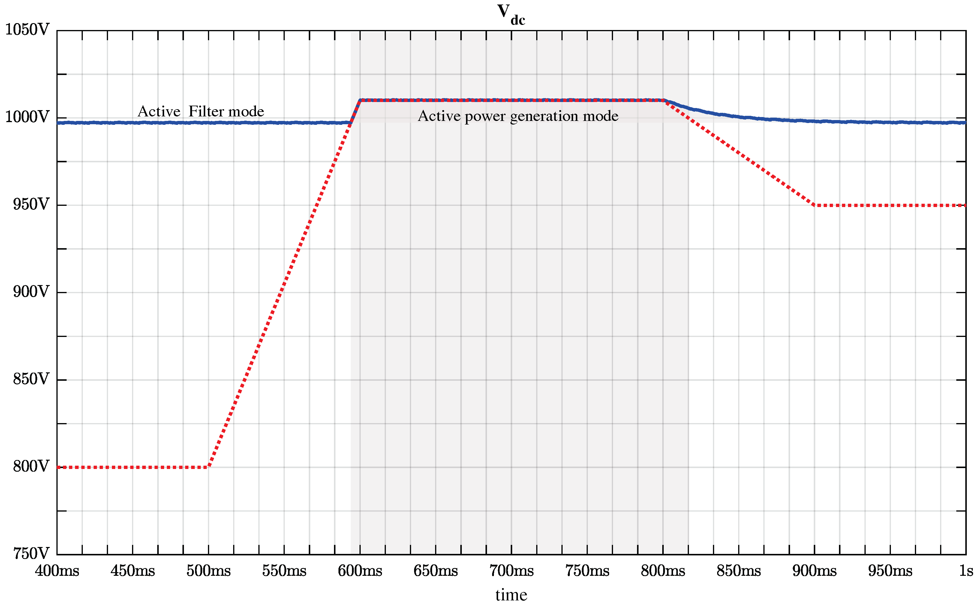
A piecewise linear source is used to represent the behavior of a photovoltaic bench; it is worth mentioning that a maximum power point tracking algorithm is not used in this investigation. The pattern of the source is selected to allow the performance of soft solar radiance. The boundary values are chosen around the operation point imposed by the control scheme. Figure 3 shows the waveform (red color) PV voltage pattern. The lower voltage value is set at 800 V for 100 ms (400 ms to 500 ms); from 500 ms to 600 ms, the voltage gradually increases to reach the upper value, settling at 1010 V. The upper voltage value is maintained for 200 ms (from 600 ms to 800 ms), and, ultimately, the voltage gradually decreases to achieve 950 V, from the time period of 800 ms to 900 ms. The voltage is fixed at 950 V until the end of the simulation.

As noted above, regulating the voltage of the DC-link capacitor is essential for the inverter to operate in active filter mode when it is impossible to transfer active power from the photovoltaic array to the electrical grid (the outside of the gray area in Figure 3). The results of this regulation, as the output power of the photovoltaic array varies, are shown in Figure 3. When the voltage of the photovoltaic array is below 1000 V (threshold voltage), the inverter acts as an active filter and maintains the voltage of the DC-link capacitor at 998 V (the set point is defined as 1000 V). Then, when the photovoltaic array voltage exceeds the threshold voltage (gray area in Figure 3), the DC-link capacitor voltage reaches the threshold voltage. Finally, when the photovoltaic array voltage falls below the threshold voltage, the voltage of the DC-link capacitor is regulated back to 1000 V. It can be said that the regulation is correct because no oscillations cause the voltage of the DC-link capacitor to drop below 1000 V, which allows the active filter function to work effectively.

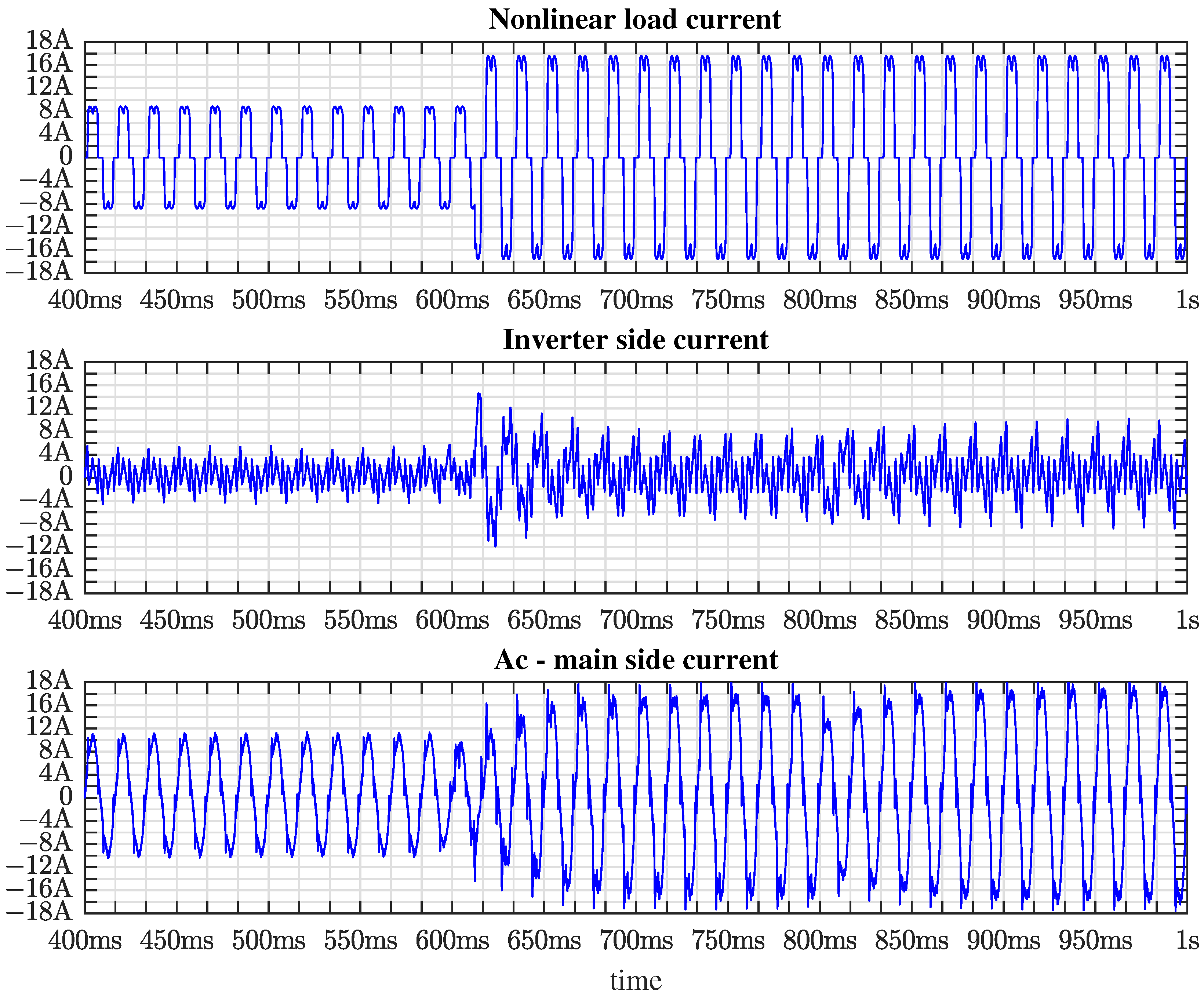
Figure 4 shows the current waveform for both inverter operating modes, that is, on the one hand, as an active filter and, on the other hand, in the injection of active power into the electrical grid, as well as the transition between them. Notice that this simulation presents a sudden load change at t = 612.97 ms to demonstrate the ability to compensate for harmonics, inject active power, and support load changes. Figure 4 shows a simulation window starting at t = 400 ms, showing the active power filter mode at approximately t = 600 ms, the inverter that supplies power to the grid, with a transient observed for 20 ms. At t = 812 ms, the inverter returns to its active filter operation, and a transient of three AC-mains cycles (≈50 ms) is also observed. These transients occur because the voltage of the DC-link capacitor changes smoothly, as seen in Figure 3. Furthermore, it is noticeable that throughout the duration covered by Figure 4, the compensated current is less distorted than the load current, indicating that the active filter function achieves its objective.

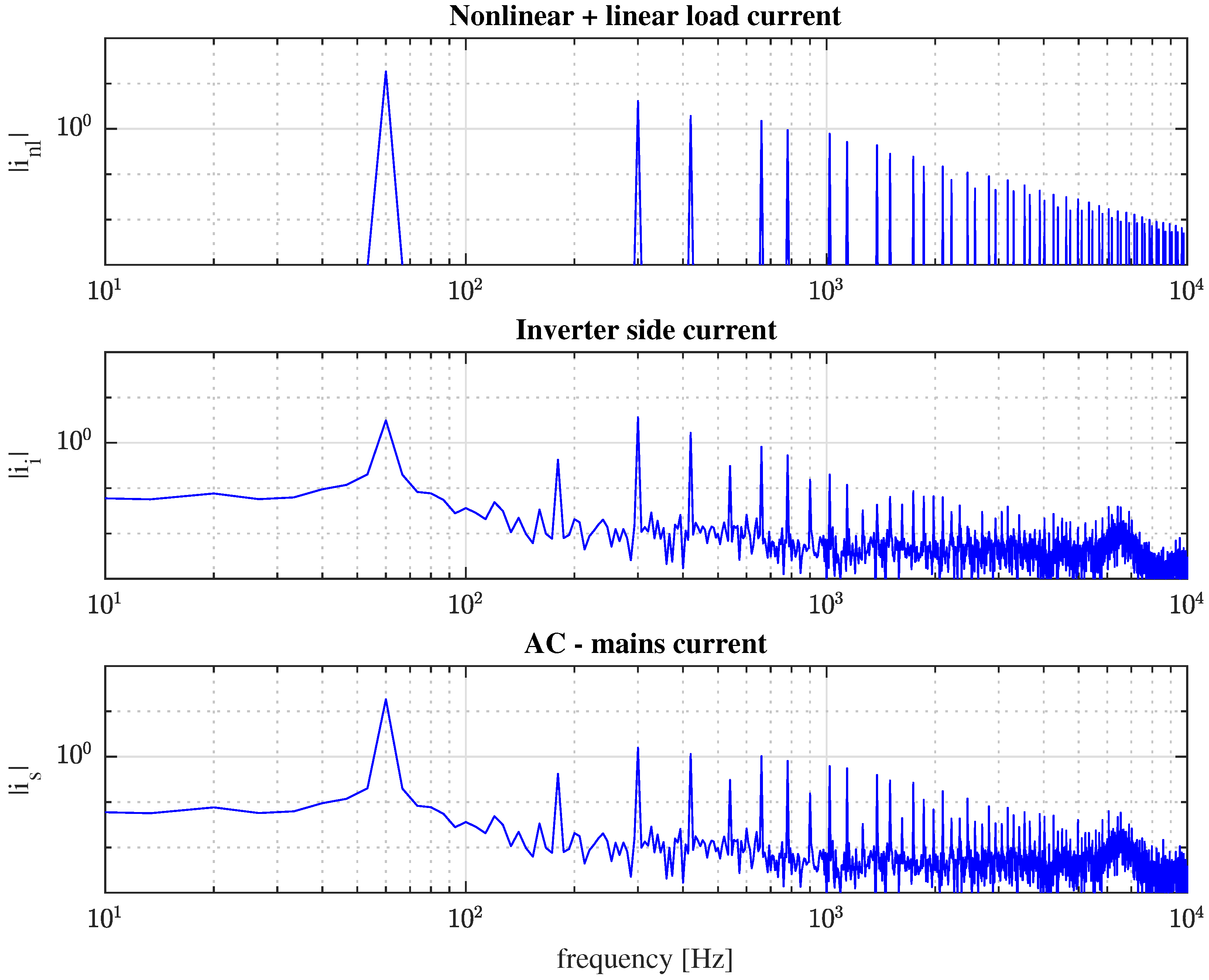
Since this work highlights the operation of the inverter as an active filter, Figure 5 shows the frequency spectrum of currents in the power converter in this mode of operation. In the upper part of Figure 5, the frequency spectrum of the nonlinear load current is shown, and it can be seen that the harmonic components have a large amplitude. A three-phase diode rectifier acts as a nonlinear load. The middle of Figure 5 shows the spectrum frequency of the compensation current generated by the inverter in its function as a current active power filter, which is used to reduce the amplitude of the harmonic components present in the load current. Finally, the current frequency spectrum injected into the AC-mains is at the bottom of Figure 5. A decreased magnitude of the harmonic components can be observed in the figure and in the following table.

Table 2. Performance results.

Harmonic	${\mathit{i}}_{\mathit{e}}^{\mathit{a}}$	${\mathit{i}}_{\mathit{e}}^{\mathit{b}}$	${\mathit{i}}_{\mathit{e}}^{\mathit{c}}$
1	$16.344$	$16.504$	$16.447$
5	$0.517$	$0.525$	$0.587$
7	$0.404$	$0.417$	$0.394$
11	$0.318$	$0.355$	$0.297$
13	$0.309$	$0.317$	$0.262$
17	$0.049$	$0.092$	$0.083$
23	$0.035$	$0.040$	$0.051$
25	$0.024$	$0.027$	$0.034$
THD	$4.86\%$	$5.02\%$	$4.96\%$

presents the FFT results related to the THD of each phase leg when the voltage source inverter acts as a current active power filter. Notice that in the results provided in the same table, each phase-leg current of the AC-mains exhibits a similar behavior. A small deviation is presented among the phase-leg currents; the deviation is due to the modeling strategy. However, it is important to note that the THD is less than 6% and is achieved according to IEEE 519-2014 [30].

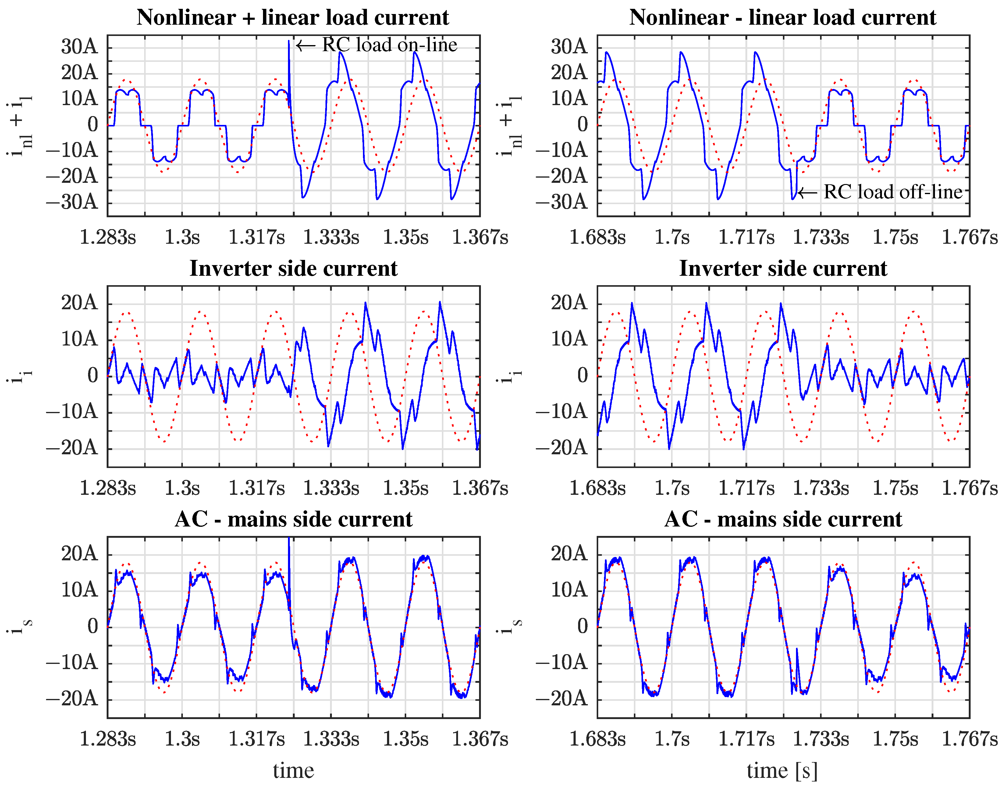
The second set of simulation results was carried out with a nonlinear load added to the RC load. In this case, a sudden load change was applied to test reactive power compensation (PFC at the fundamental frequency). Therefore, polluted current signals contain harmonics and fundamental delays associated with RC-load (high capacitive load). In Figure 6, a nonlinear load is connected to the PCC, the THD before the reactive load is approximately 4.9%, and the power factor PF = 0.991. At t = 1.324 s, an RC load is connected, the THD is 4.2%, and the power factor is ≈0.995. For a few milliseconds, the load is the sum of a nonlinear and a linear load. At t = 1.728, the linear load is offline and the power converter operation begins. In Figure 6, from top to bottom, the oscillograph shows the nonlinear load in blue, and the superimposed dotted red line is the AC-mains voltage ten times downscale. Both sides represent when the linear load is connected in parallel and disconnected from a nonlinear load. At the center of the same figure, the current generated by the inverter is shown. A superimposed sinusoidal waveform shows the phase shift between the current and the AC-mains voltage. Finally, at the bottom, the compensated current is shown. As can be seen, the power factor is close to 1 and confirms the purpose of the investigation.

5. Conclusions

This paper presents the development of a model-based control scheme. The switching function is integrated into the model to preserve nonlinearity, enabling a sliding mode controller to be involved. In addition, an observer based on the methodology of immersion and invariance is used. An external control loop is introduced to regulate the DC-link voltage in the power electronic converter. Beyond its function as an active power filter, the converter is also designed to deliver active power generated by a PV array. The control scheme includes a decision loop that manages operations based on solar irradiance availability. During the day, the inverter is powered by PV panels, which directly use energy from the array. At night, the control scheme disconnects the PV panels, and the inverter operates exclusively as an active power filter, providing reactive power compensation (at the fundamental frequency) and power factor correction. The simulation results demonstrate effective regulation, reducing the harmonic distortion in the current injected into the electrical grid from $27.5\%$ to $5.02\%$. These results confirm the efficacy of the proposed control scheme in achieving the desired system performance. In both modes of operation, the high total harmonic distortion (THD) caused by nonlinear load connections is effectively mitigated, ensuring that the current injected into the grid is significantly less distorted than the load current. Furthermore, simulations carried out with an RC load combined with a nonlinear load show that the power factor remains close to unity, reinforcing the research objectives of harmonic compensation and power factor correction.