Article

Stability Boundary Characterization and Power Quality Improvement for Distribution Networks

1
College of Electrical Engineering, Zhejiang University, Hangzhou 310027, China
2
State Grid Shanxi Electric Power Research Institute, Taiyuan 030001, China
*
Author to whom correspondence should be addressed.
Energies 2024, 17(24), 6215; https://doi.org/10.3390/en17246215
Submission received: 30 September 2024 / Revised: 15 November 2024 / Accepted: 21 November 2024 / Published: 10 December 2024
(This article belongs to the Section F: Electrical Engineering)

Abstract

:
With the increasing proportion of distributed generators (DGs), distribution networks usually include grid forming (GFM) and grid following (GFL) converters. However, the incompatibility of dynamic performance caused by different control methods of the GFM and GFL converters may bring instability problems and power quality risks to the distribution network. To solve this issue, the models of the GFM and GFL converters are established first to lay a good foundation for stability analysis and power quality improvement control. On this basis, an inner loop parameters design scheme is developed for GFM converters based on the D-Partition method, which facilitates the stability boundary characterization. Meanwhile, a current injection strategy is proposed to enhance the voltage support capacity of the GFL converter during grid faults. Moreover, for the distribution network with multi-converters, a compensation current control based on the analytic hierarchy process and coefficient of variation is proposed to ensure a balance between minimal capacity and optimal power quality. In this manner, DGs can be plug-and-play without considering stability and power quality issues. Finally, the effectiveness of the proposed strategy is validated with simulation results.

1. Introduction

The growing penetration of renewable energy has led to the widespread application of grid-connected converters in power systems, which are divided into grid forming (GFM) and grid following (GFL) converters [1,2,3]. GFM converters need to control the frequency and voltage of the islanding system [4], while GFL converters can deliver constant power to the system to maximize the use of renewable energy generation [5,6]. However, due to the different control schemes of the GFM converter and GFL converter, their dynamic performance is usually incompatible. As a result, the cascade system easily loses stability and decreases the power quality under disturbances.
The inner loop of GFM converters typically employs dual-loop control for voltage and current. Improper parameter settings in the inner loop are a primary cause of output oscillations in GFM converters. Common methods for designing inner loop parameters include the traditional system tuning method, pole-zero configuration method, and symmetrical optimal method [7,8,9]. Then, the performance of the converter is typically evaluated using the Routh criterion, Nyquist plot, and Bode plot. This process is complicated and often requires repeated adjustments [10,11,12]. Therefore, the instability issue of the GFM converter needs to be further addressed.
GFL converters are not only required to remain connected to the grid during fault conditions but also to autonomously support the voltage at the point of common coupling (PCC) by controlling the dual-sequence reactive current [13,14]. During grid faults, the injected current reference can be generated from multiple optimization objectives, including minimizing power oscillations, reducing converter fault currents, and ensuring compliance with phase voltage limits. A current injection strategy is proposed [15] to mitigate the overcurrent risk by introducing a predefined constraint. Taking the current constraint into consideration, an algorithm is proposed [16] to maximize the converter output capability during faults, which effectively avoids active power oscillations. Furthermore, a current reference optimization method based on second-order cone programming is introduced to deal with the unbalanced voltage under asymmetrical faults [14]. However, these methods are only suitable for asymmetric faults, and the voltage support capacity of the converter remains unclear.
The stability and reliability of power systems are primarily associated with factors such as reactive power compensation, harmonic pollution, three-phase imbalance, voltage fluctuations, and network security [17]. Among these challenges, we specifically focus on the first three most typical issues [18]. Due to the location and capacity limitations of power quality management devices, the management effect of only one device is limited. Thus, it is necessary to study the coordinated control of multiple inverters to improve the power quality in distribution networks. A comparative analysis of key metrics-adaptability, computational efficiency, and robustness—enables a clearer comparison between the proposed model and other methods like predictive modeling and multivariate techniques. This broader analysis aims to better understand the strengths and limitations of different approaches in managing distributed systems effectively to explore resource distribution and structural changes in distributed systems [19]. A centralized control scheme is proposed in [20], where a control center dispatches commands to all inverters to adjust their power factor and harmonic compensation, but this method would increase the number of controllers and sensors [21]. To solve this problem, converters need to balance the importance of different indicators adaptively. In [22], some problems of the contemporary economy associated with decision-making under uncertainty are analyzed based on the theory of approximations. This theory may be applied to power quality management because the compensation of converters depends on various factors, and the overall demand for compensation in power quality issues is uncertain. However, it requires the use of complex mathematical calculations and models and is not suitable for direct application in the power system. For this, hybrid weighting is proposed to balance the importance of different indicators in a much simpler and more acceptable way. Nevertheless, allocating the excess compensable capacity also brings great challenges to the multi-inverter system [23].
This paper focuses on the stability-oriented design of controller parameters and power quality improvement for distribution networks. The main contributions of this paper are summarized as follows.
  • A D-Partition-based controller parameter design method is proposed for GFM converters, which can determine the Proportional Integral (PI) parameter stability domain that meets the requirements of phase margin, gain margin, and short circuit ratio.
  • A current reference generation strategy is proposed to generate positive-sequence and negative-sequence reactive current commands considering the capacity limitations of the GFL converter and switch devices, which effectively achieves adaptive current limitations.
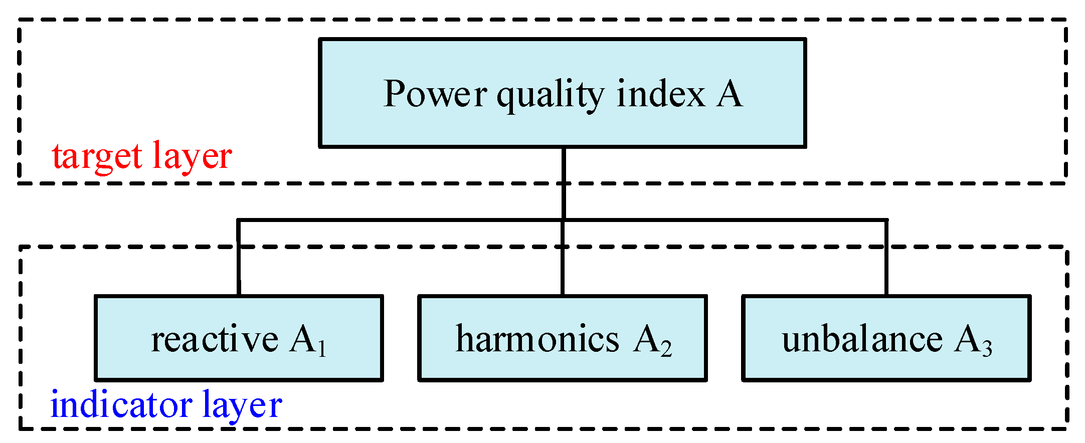
  • In a multi-converter system, a compensation current control based on the analytic hierarchy process (AHP) and the coefficient of variation (CV) is proposed to achieve the balance between minimum capacity and optimal power quality.
The rest of this paper is organized as follows. A brief description of a distribution network and the modeling of the GFM converter and GFL converter are given in Section 2. The stability boundary of the GFM converter is characterized based on the D-Partition method in Section 3. The proposed current reference generation method and compensation current control are highlighted in Section 4 and Section 5. Section 6 presents the case validations in MATLAB/Simulink (MathWorks, Natick, MA, USA). Finally, Section 7 presents the conclusions.

2. System Description and Modeling

A classical structure diagram with multiple distributed generators (DGs) is first introduced in this section. Then, the detailed model of the GFM converter and GFL converter is established, which lays a good foundation for the system stability analysis and power quality improvement.

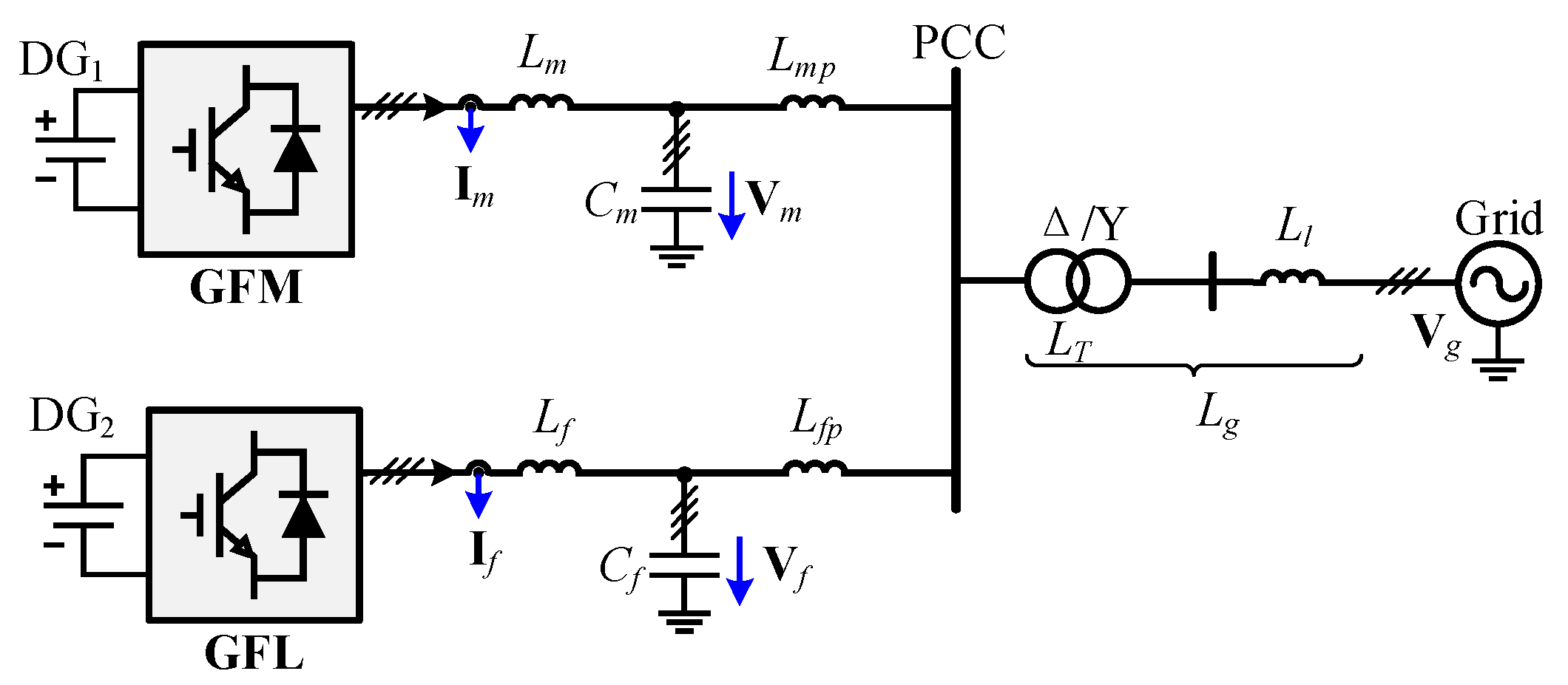
2.1. System Description

A typical diagram of a grid-connected power conversion system is shown in Figure 1 [24,25,26], where the grid is simplified as an ideal AC voltage source Vg in series with an equivalent grid inductance Lg, and Lg is composed of transformer inductance LT and transmission line inductance Ll. The transformer used is a Δ/Y transformer, which effectively eliminates the zero-sequence component in the three-phase system. According to the different control targets, the converters in the grid-connected system can be divided into GFM converter and GFL converter.
The terminal voltage of GFM converters typically uses an inner dual-loop control structure, which includes an outer voltage loop and an inner current loop, as shown in Figure 2 [27]. udref and uqref represent the d-axis and q-axis components of the voltage loop reference, respectively. θc is the phase derived from the droop control for power synchronization, which is determined by the output power Pe and the reference power P0.
The control unit of the GFL converter is mainly composed of four components, including a double second-order generalized integrator phase-locked loop (DSOGI PLL), a current reference generator, and an inner current loop, as presented in Figure 3. The DSOGI PLL is utilized to obtain the phase angle θ of the PCC voltage Vf. The current reference generator block generates current reference (iaref and ibref) in the ab frame according to θ of PCC, active power reference P* and AC voltage command Vf*. The inner current control is implemented in the ab frame, utilizing proportional-resonant (PR) controllers to realize zero-error current reference tracking.

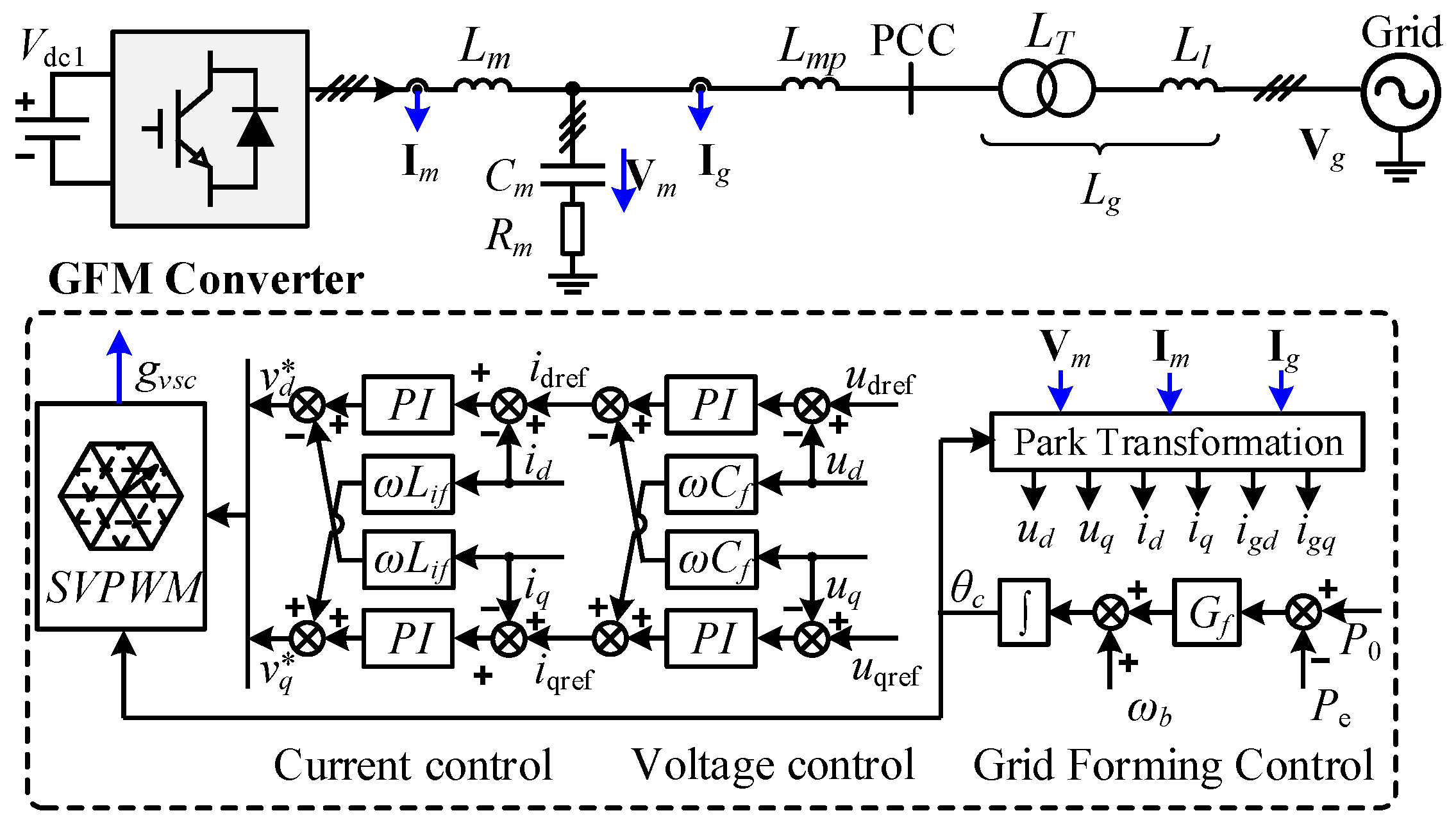
2.2. Modeling of GFM Converter

Currently, the main types of GFM control technologies include droop control, virtual synchronous generator (VSG), and virtual oscillator control (VOC). The traditional droop control equation is shown in Equation (1). This control equation mimics the power transmission characteristics in power systems, where active power has a linear relationship with frequency, and reactive power has a linear relationship with voltage.
{ ω = ω r e f + K p ( P r e f P ) U = U r e f + K q ( Q r e f Q ) θ = ω d t
where Pref is the reference value for the active power output of the converter, P is the actual active power output of the converter, ωref is the reference angular frequency for the converter output, ω is the actual output angular frequency of the droop-controlled converter, θ is the output phase angle of the droop-controlled converter (obtained by integrating the actual angular frequency), Kp is the active power droop coefficient, Qref is the reference reactive power output of the converter, Q is the actual reactive power output, Uref is the reference output voltage magnitude, U is the output voltage magnitude of the droop-controlled converter, and Kq is the reactive power droop coefficient.
By measuring the converter output voltage and current, the active power P and reactive power Q are calculated, which serve as inputs to the droop control loop. Through the droop characteristics, the phase angle θ and voltage magnitude U are determined, which are then used as the reference voltage for the outer voltage loop in the subsequent dual-loop voltage and current control. The block diagram for droop control is shown in Figure 4.
The frequency of security incidents in modern power systems has risen due to low grid inertia. Traditional synchronous generators provide inertia for frequency stability, a function VSGs now emulate by converting DC to AC while offering inertia support. Voltage-controlled VSGs are better suited for weak grids, microgrid islanding, and renewable integration than current-controlled types.
The active power control loop equation for VSG can be expressed as
{ P m P ref = K ω ( ω ω ref ) P m ω ref P e ω ref D ( ω ω ref ) = J d ω d t θ = ω d t
where Pm is the mechanical power output of the virtual rotor, Pref is the reference active power, Pe is the electromagnetic power, Kω is the droop coefficient, ω is the output angular frequency of the virtual synchronous machine, ωref is the reference angular frequency, and θ is the output phase angle of the virtual synchronous machine.
The reactive power control loop of VSG can adopt a similar form to droop control. The active power control loop outputs the phase angle θ, while the reactive power control loop outputs the voltage magnitude U. θ and U provide the reference voltage for the outer voltage loop in the dual-loop voltage and current control, as shown in Figure 5.
In droop control and VSG control, the reference voltage for the dual-loop voltage and current control is computed by the outer power controller based on the power sampling results. In contrast, in VOC, the reference voltage is generated by a virtual oscillator. The oscillator is a physical resonant circuit, while the virtual oscillator is modeled through differential equations and discretized into a virtual circuit via programming. VOC-based parallel converters can achieve synchronization without communication between converters, thanks to their self-synchronizing properties. However, voltage magnitude and phase angle mismatches in parallel systems can cause circulating currents.
The virtual oscillator comprises an LC oscillating circuit, a controlled current source combined with a controlled resistance module (SRM), and a current-controlled current source. The control block diagram of the VOC strategy is shown in Figure 6.
As summarized in Table 1, the three grid-forming control techniques exhibit distinct characteristics, making them suitable for different operating conditions. Droop control, while functional in both grid-connected and islanded modes, lacks inertia support and damping mechanisms. This absence of inertia results in fast adjustment responses under power or frequency fluctuations, which, although beneficial in certain scenarios, can increase the risk of frequency instability, particularly during disturbances. Despite its simplicity and quick response, droop control’s moderate current-sharing capabilities may limit its effectiveness in systems with varying load demands.
VSG addresses many of the shortcomings of droop control by introducing inertia and damping support, mimicking the dynamic behavior of traditional synchronous generators. These features significantly enhance system stability during dynamic adjustments, making VSG more robust under both grid-connected and islanded conditions. However, the added complexity of simulating virtual inertia results in slower response times compared to droop control, and its current-sharing capability, while stable, remains moderate and comparable to droop control.
VOC stands out for its self-synchronizing property, which enables seamless synchronization among parallel converters without requiring communication between units. This feature enhances current sharing significantly, making VOC highly effective for multi-converter parallel operations. Additionally, its fast response time is comparable to droop control, making it well-suited for systems that demand rapid adjustments. However, VOC’s tendency to produce higher harmonics during grid-connected operation can impact power quality, which limits its applicability in purely grid-tied scenarios.
In summary, droop control offers simplicity and quick response but lacks the robustness required for dynamic grid stability. VSG provides improved stability and damping, making it ideal for systems requiring strong inertia support, albeit at the cost of slower response. VOC, with its superior current-sharing capabilities and fast response, is particularly suitable for decentralized and multi-converter systems, though its harmonic output must be considered in grid-tied applications. Each technique offers unique advantages, and their selection should be tailored to the specific requirements of the system.
The outer loop of the GFM control achieves power regulation and grid synchronization by emulating the active power frequency and reactive power-voltage droop characteristics of a synchronous generator. Considering that the control bandwidth of the outer loop is much smaller than the inner loop, the dynamics of the outer control loop can be neglected in this study.
Using the harmonic linearization method, the three-phase system is decomposed into positive and negative sequence subsystems. According to the impedance stability criterion [28,29,30,31], the stability of the positive sequence subsystem is essential for the overall stability of a GFM converter. Thus, the control block diagram of the positive sequence subsystem for a GFM converter is illustrated in Figure 7.
Based on Figure 7, the output voltage can be expressed as
u f ( s ) = T ( s ) 1 + T ( s ) u r e f ( s ) Z o ( s ) i g ( s )   = Φ ( s ) u r e f ( s ) Z o ( s ) i g ( s )
where T(s), Φ(s) and Zo(s) are the open-loop transfer function, closed-loop transfer function, and output impedance of the GFM converter, respectively. They are expressed as
T ( s ) = G v ( s j ω 0 ) K p i G d ( s ) + G d ( s ) 1 + s 2 L m C + s C K p i G d ( s ) G d ( s )
Φ ( s ) = G v ( s j ω 0 ) K p i G d ( s ) + G d ( s ) 1 + s 2 L m C + s C K p i G d ( s ) + G v ( s j ω 0 ) K p i G d ( s )
Z o ( s ) = s L m + K p i G d ( s ) 1 + s 2 L m C + s C K p i G d ( s ) + G v ( s j ω 0 ) K p i G d ( s ) + s L g
In Equations (4)–(6), Gv(s) = Kpv + Kiv/s represents the PI regulator of the outer voltage loop. C = Cm /(sCmRm + 1) represents the equivalent capacitance. Kpi is the proportional gain of the inner current control loop. Gd(s) = e−sTs(1−e−sTs)/(sTs) represents the digital control delay [32], where Ts is the sampling period of the GFM converter.

2.3. Modeling of GFL Converter

Under normal conditions, the GFL converter always delivers active power to the grid. However, during grid fault conditions, such as the three-phase short circuit fault or single-phase short circuit fault, the converter must inject appropriate reactive power to support the PCC voltage. The relationship between the PCC voltage and the grid voltage is given as follows.
V f = V g + L g d I f d t
Since symmetrical faults in the grid can be considered as a specific case of asymmetrical fault, only the modeling of asymmetrical fault is required. Under asymmetrical fault conditions, PCC voltage (Vf) and the grid current (If) become asymmetrical, containing both positive and negative sequence components. To facilitate analysis, only the fundamental frequency components of the voltage and current are considered; thus, the dual-sequence components are shown in Equations (8) and (9), where superscripts “+” and “−” denote the positive and negative sequence components, respectively; φu+ and φu are the initial phase angles of the positive and negative sequences of voltage Vf; φi+ and φi are the initial phase angles of the positive and negative sequence of If; ω is the angular velocity of the grid.
V f = V f + e j ( ω t + φ u + ) + V f e j ( ω t + φ u )
I f = I f + e j ( ω t + φ i + ) + I f e j ( ω t + φ i )
According to Equations (8) and (9), (7) can be decomposed into two components as follows.
{ V f + = V g + + j ω L g I f + V f = V g j ω L g I f
According to Equation (10), the relative position between the PCC voltage vector (Vf+, Vf) and grid voltage vector (Vg+, Vg) is determined by the current vector (If) location, as shown in Figure 8.
As illustrated in Figure 8a, the positive sequence current vector (If+) located in the orange region can enhance the positive sequence PCC voltage vector (Vf+) while decreasing the PCC voltage when the current vector is located in the blue region. Similarly, as shown in Figure 8b, the negative sequence current vector (If) located in the orange region can decrease the negative sequence PCC voltage vector (Vf) while increasing the PCC voltage when the current vector is located in the blue region.
Thus, to realize optimal support performance of PCC voltage, the positive sequence current should lag the positive sequence vector of PCC voltage by 90°, as shown in Figure 9a. On the contrary, the negative sequence current should lead the PCC voltage negative sequence vector by 90°, as depicted in Figure 9b.

2.4. Comparison Between GFL and GFM Converter

GFL and GFM converters, though sharing similar topologies by converting DC power to AC through power electronics, differ significantly in their control strategies, affecting their roles within the power grid. The primary goal of GFL converter control is to inject power into the grid, while grid support is a secondary function. GFL converters operate by following the existing grid’s voltage and frequency, effectively behaving as controlled current sources. This approach limits their capacity to provide dynamic support for grid stability, particularly in systems where the grid is weak or faces high levels of renewable energy integration.
In contrast, GFM converters are designed not only to inject power but also to actively support and stabilize grid parameters such as frequency and voltage. This function becomes particularly valuable in modern power systems, which face both high renewable penetration and high power demand. Grid stability and immunity to disturbances are critical, and the ability of GFM converters to regulate and stabilize the grid provides a key advantage, making it an increasingly important choice for modern power systems.
A key distinction between GFL and GFM converters lies in their control variables. GFL converters control current by employing PLL to align with the grid voltage phase angle. This approach enables GFL converters to function as current-controlled sources in parallel with the grid. However, under weak grid conditions, the dependence on PLL can introduce stability issues, with oscillations and harmonics affecting system stability. On the other hand, GFM converters manage the voltage phase angle and amplitude directly without requiring a PLL for synchronization. This absence of PLL improves their stability, especially under weak grid conditions, as GFM converters can independently establish their reference phase angle. This feature makes GFM converters more resilient to grid disturbances, reducing harmonic oscillations and enhancing overall system stability.
In essence, while GFL and GFM converters share structural similarities, their control differences lead to distinct functional roles. GFL converters are suited for applications prioritizing power injection, though they offer limited support in weak grid conditions. GFM converters, however, stand out for their robust support in grid-forming applications, providing the resilience and stability crucial to modern power systems with high renewable energy integration [33].

3. Stability Boundary Characterization Based on D-Partition Method

In this section, the principle of the D-Partition method is introduced first. On this basis, the inner loop controller of the GFM converter is designed based on the D-Partition method, which makes the system stability meet multiple performance criteria such as phase margin (PM), gain margin (GM), and short-circuit ratio (SCR). This method allows for the quick and accurate determination of inner loop control parameters through graphical visualization, thus eliminating the need for repetitive trial-and-error adjustments.

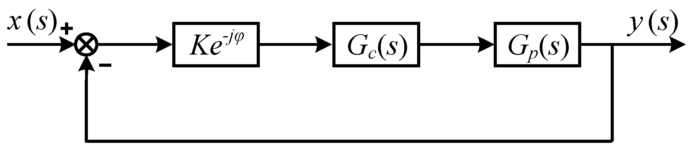
3.1. Principle of D-Partition Method

The core principle of the D-Partition method is to establish a direct relationship between the variable parameters of the closed-loop characteristic equation and the stability region of the controller [34]. As ω varies from −∞ to +∞, the D-Partition boundaries in the controller parameter space are constructed by mapping the (−1, j0) to the parameter space. By clearly defining these stability boundaries, this method facilitates the accurate design of inner loop controllers to maintain system stability [35].
To address the importance of system stability and performance analysis, the D-Partition method is used to characterize stable regions for the controller parameters in GFM converters. This method ensures that key criteria such as phase margin (PM), gain margin (GM), and short-circuit ratio (SCR) are met, enabling a comprehensive evaluation of both dynamic and steady-state performance. The D-Partition method provides a quick and accurate determination of inner loop control parameters without requiring extensive iterative adjustments, significantly enhancing the robustness and reliability of the system under varying operating conditions.
Figure 10 illustrates a unity feedback system with a PI controller, where x(s) and y(s) represent the reference signal and the actual output of the system, respectively. Gc(s) represents the PI controller, and Gp(s) represents the controlled plant. The expressions for these components are given by
{ G c ( s ) = K p + K i s G p ( s ) = a n s n + a n 1 s n 1 + + a 1 s 1 + a 0 b m s m + b m 1 s m 1 + + b 1 s 1 + b 0
where Kp and Ki represent the proportional and integral items of the PI controller, respectively. The coefficients ai for i = 0, 1, 2, …, n and bj for j = 0, 1, 2, …, m correspond to the numerator and denominator polynomials of Gp(s). Thus, the closed-loop characteristic equation of the system is expressed as
D ( s , K p , K i ) = s ( b m s m + b m 1 s m 1 + + b 1 s 1 + b 0 ) + ( s K p + K i ) ( a n s n + a n 1 s n 1 + + a 0 )
Based on the principles of the D-Partition method, the boundaries of the D-Partition can be expressed as
{ D ( 0 , K p , K i ) = 0 D ( , K p , K i ) = 0 D ( ± j ω , K p , K i ) = 0
where ω is the rated angular frequency of the system, and D represents the closed-loop characteristic equation of the system.
In a control system, a phase-gain margin tester Ke−jφ is added for flexible adjustments to obtain the corresponding PM and GM, as shown in Figure 11. K represents the GM of the system, with GM = 20 lgK, and φ represents the PM of the system, with φ = PM.

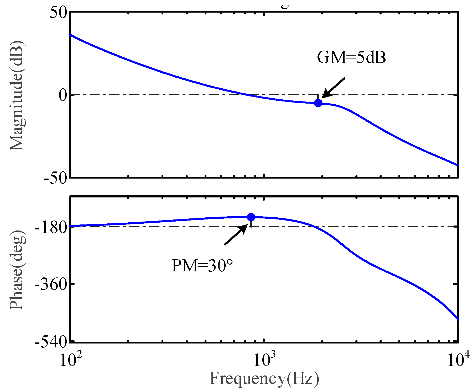
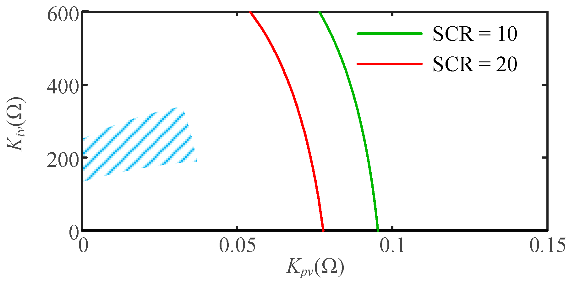
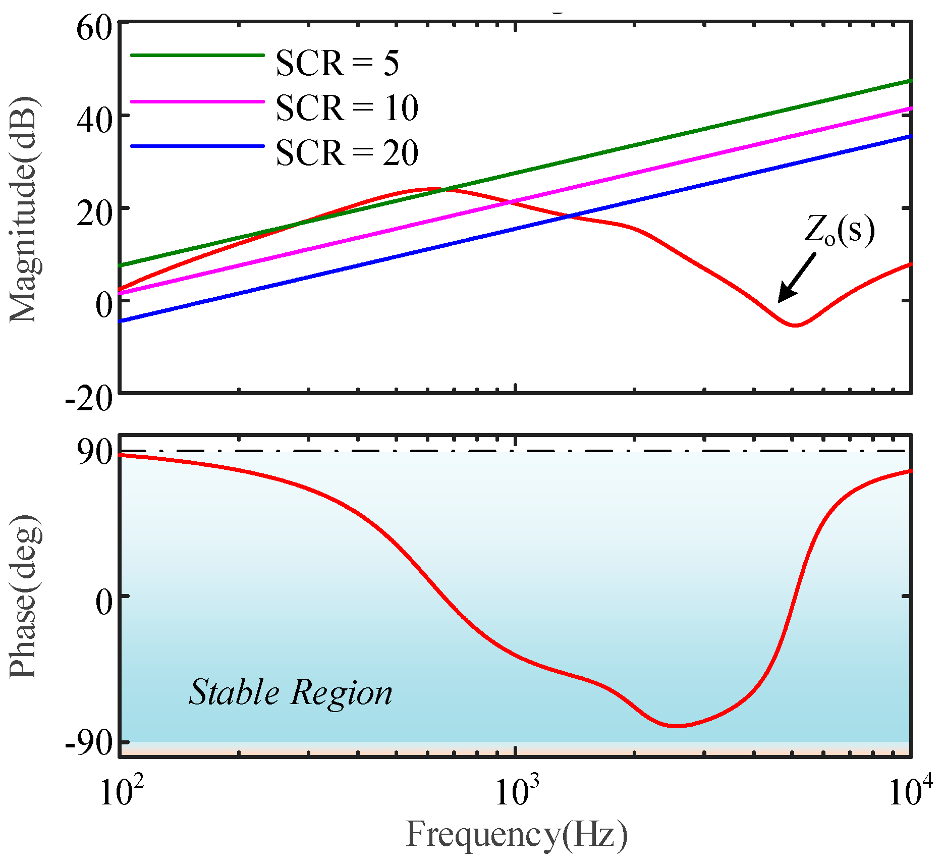
3.2. Stability Boundary Characteristics of GFM Converter

To design the feasible region for the inner loop parameters of the GFM converters, the closed-loop characteristic equation is derived first as Equation (14) according to Equation (5).
D ( s ) = [ K p v ( s j ω 0 ) + K i v ] ( 1 e ( s T s ) ) e ( s T s ) K p i                                                             + ( s j ω 0 ) [ s T s + s 3 L m T s C + s C ( 1 e ( s T s ) ) e ( s T s ) K p i ] )
Substitute s = ± into the closed-loop characteristic equation and solve for the PI parameters as a function of ω. By varying ω from −∞ to +∞, the calculated Kpv and Kiv values can be described in Figure 12. Utilize a phase-gain margin tester to determine the stable region that satisfies the gain margin GM ≥ 5dB and phase margin 30° ≤ PM ≤ 45°, as shown in the shaded area in Figure 12. This means that the dynamic and steady-state performance of the GFM converter under ideal grid conditions can be ensured as long as the PI parameters are selected within this shaded area, regardless of the grid impedance.
Selecting any point on the curve, such as (0.0322,334) in Figure 12, and substituting it into Equation (4). Then, the Bode plot of the corresponding open-loop transfer function can be obtained, as shown in Figure 13. It can be seen that the GFM converter achieves a PM of 30° and a GM of 5 dB, which validates the accuracy of the D-Partition method.
When the grid impedance is considered, the GFM converter and the grid can be modeled as a cascaded system, and the impedance stability criterion is used to evaluate its stability. Based on Equation (6), the PI parameter domains corresponding to SCR values of 10 and 20 are obtained, as shown in Figure 14. As the SCR decreases, the stable domain of the PI parameters gradually shrinks, which indicates that the stability boundary of the GFM converter becomes narrower as the grid strength decreases.
As shown in Figure 14, the PI parameters selected within this shaded region can ensure that the GFM converter maintains impedance stability when the SCR value is less than 20. To validate the impedance stability of the parameters, the Bode diagram of Zo(s) is obtained with the PI set to (0.02, 250), as shown in Figure 15.
In summary, under weak grid conditions, as long as the parameters of the PI of the GFM converter are within the shaded area shown in Figure 14, the inner loop control parameters can meet multiple performance constraints, including GM ≥ 5dB, 30° ≤ PM ≤ 45°, and SCR < 20. This approach effectively ensures that the converter can maintain dynamic and steady-state performance even under challenging grid conditions.

4. Positive and Negative Current Reference Generator

In this section, a current injection strategy based on a voltage droop control method is proposed to realize flexible and dynamic allocation of positive and negative sequence currents. It is worth noting that the proposed current injection strategy takes the inherent constraints of the converter into consideration and incorporates adaptive current limitation capabilities.

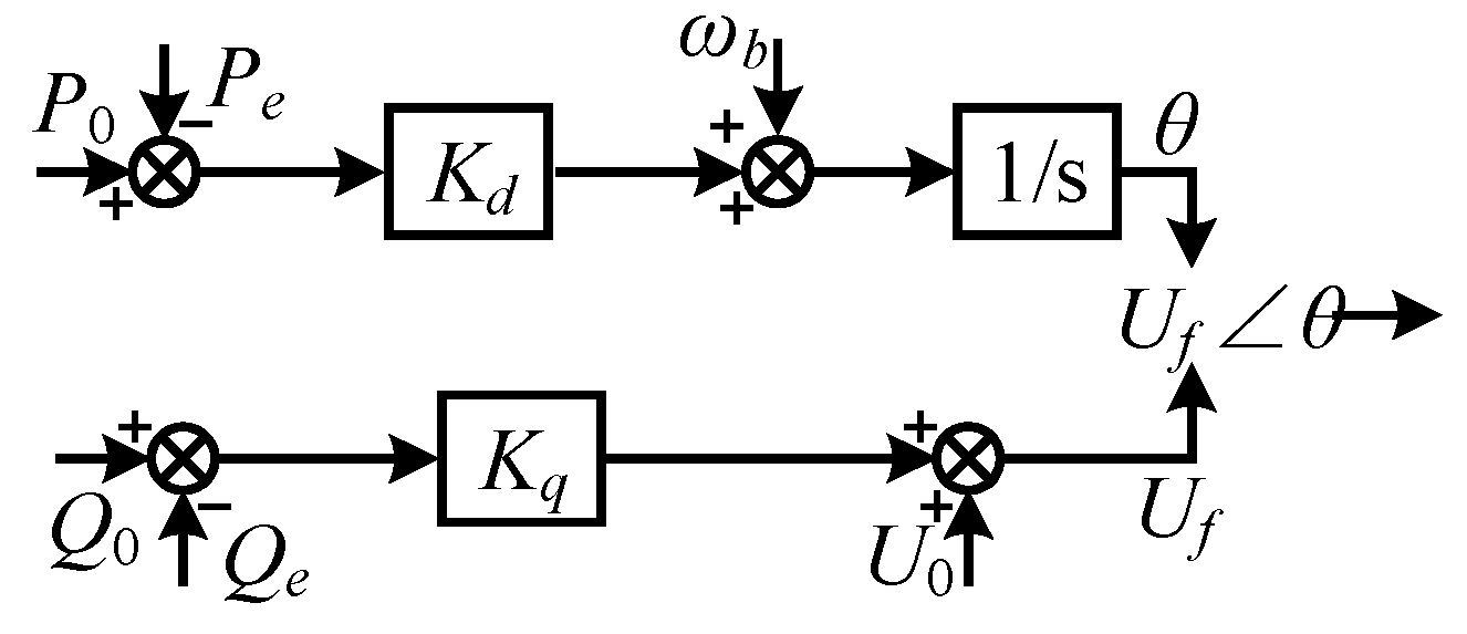
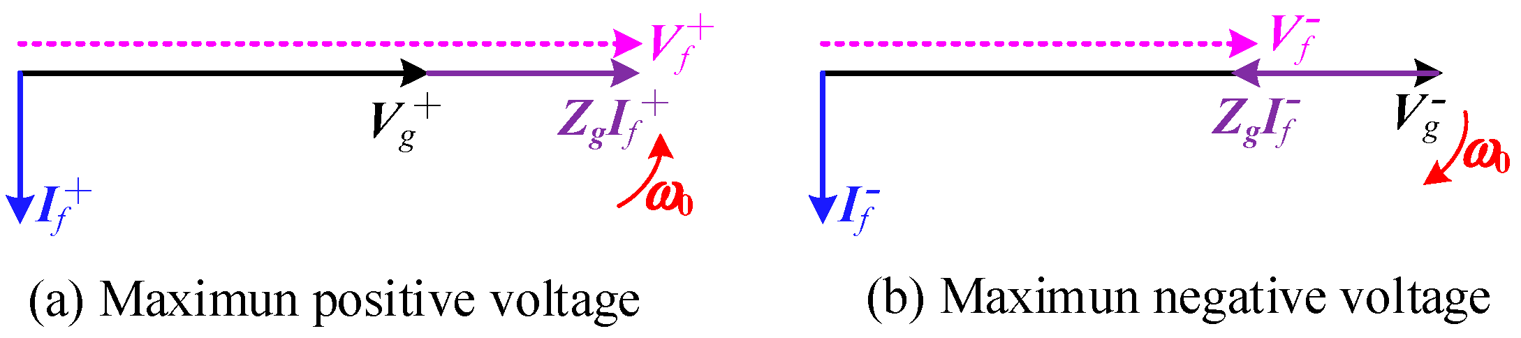
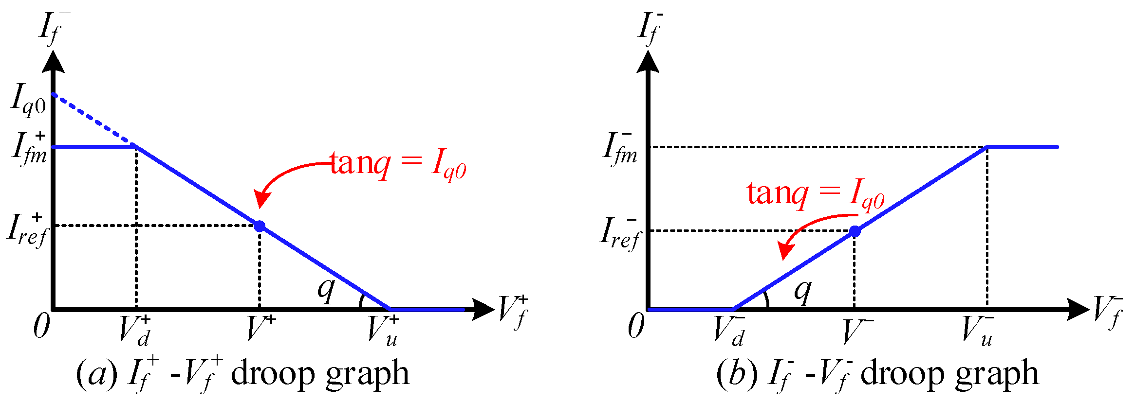
4.1. Current Generator Based on Voltage Droop Control

The GFL converter is designed according to the specific grid system so the normal value of the PCC voltage can be confirmed. Simultaneously, the line impedance can be obtained through online estimation. To support the PCC voltage within the normal range, the droop curve of the positive sequence reactive current Iref+ and the positive sequence voltage V+ can be constructed based on Equation (10), as present in Figure 16a. Similarly, the droop curve of the negative sequence reactive current Iref and the negative sequence voltage V is also depicted in Figure 16b. These droop curves can be used to generate corresponding positive and negative sequence reactive current references during grid faults.
In Figure 16, Iq0 represents the reactive current required to support the PCC voltage at its rated value during the three-phase-to-ground fault. Vu+ is the minimum positive sequence component, and Vd is the maximum negative sequence component of the PCC voltage within normal boundaries. Considering the constraints of the GFL converter, Vd+ and Vu represent the minimum positive sequence voltage and the maximum negative sequence grid voltage that the converter can stand the PCC voltage in the normal range, respectively. V+ and V represent the positive and negative sequence components of the voltage during a grid fault. Based on Figure 16a and Figure 16b, the expressions of the positive and negative sequences of the reactive current references are given as follows.
I r e f + = { 0 , V + > V u + ( V u + V + ) I q 0 , V d + V + V u + I f n + , V + < V d +
I r e f = { 0 , V < V d ( V V d ) I q 0 , V d V V u I f n , V > V u
where the short-circuit current Iq0 is expressed as
I q 0 = V N / ω L g
Thus, when a grid fault occurs, the GFL converter can realize the PCC voltage support by generating corresponding positive and negative sequence reactive current according to the strategy depicted in Figure 16.

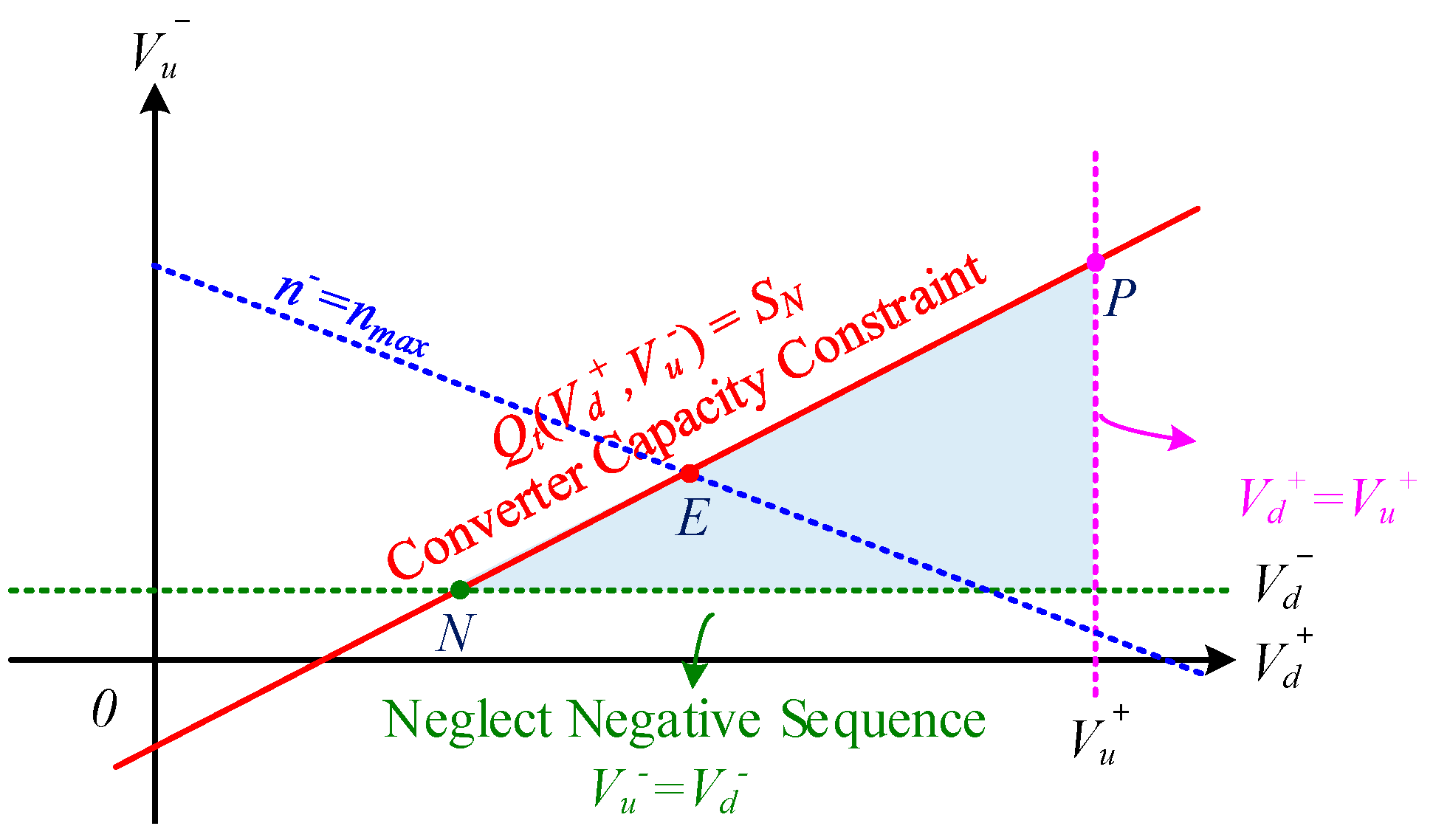
4.2. Limits of Converter Capacity

The power electronic-based converters have limited overcurrent output capacity due to the vulnerability of semiconductor devices. When the grid voltage drop is light, the positive and negative sequence reactive current commands generated by Equation (10) do not reach the operational boundaries of the GFL converter. However, in cases of severe voltage drop or severe asymmetry faults, the three-phase currents may reach the safety operation boundaries of the device. As a result, the current references must be limited according to the constraints of the converter; otherwise, the device may be damaged. Thus, the converter needs to support the PCC voltage with its maximum capacity.
The strategy for limiting the positive and negative sequence reactive current is elaborated as follows. Firstly, with the relationship between the output current and the PCC voltage derived in Equation (10), the current limitation is expressed by the relationship between the PCC voltage and the grid voltage.
Considering the capacity limitation to support the PCC voltage, it is essential to delineate the grid fault boundaries. According to Equations (15) and (16), (Vd+, Ifm+) and (Vu, Ifm) characterize the fault boundary values corresponding to the capacity to support the PCC voltage and determine the total reactive capacity Qt. Qt should not exceed the rated capacity (SN), which is expressed as follows.
Q t ( V d + , V u ) S N
According to the theory of instantaneous power, the expressions of active power and reactive power injected into the grid can be expressed as Equations (19) and (20), respectively. Under asymmetric faults, both the active power P and reactive power Q contain the average component and the power oscillation component.
P ( t ) = V f I f
Q ( t ) = V f I f
Given that (Vd+ Vu) represents the boundary points, the positive and negative sequence components of the PCC voltage can still be restored to their normal values. Neglecting the influence of power oscillations, Qt can be expressed as
Q t = 3 2 ( V u + I f m + + V d I f m ) V N
Combining Equations (18) and (21), Equation (18) can be further simplified as
V d V u V u + V d + Q N 3 V N I q 0 / 2 ( V u + 2 V d 2 ) M
Obviously, Vu+ is higher than Vd+, and Vd is lower than Vu. This relationship depicts the feasible region characterized by (Vd+, Vu). The functional expression of the feasible region is provided in Equation (23). Accordingly, the feasible region of (Vd+, Vu) can be described in Figure 17.
{ V d V u V u + V d + M 0 V d + V u + V u V d 0
It can be seen from Figure 17 that when the coordinate point (Vd+, Vu) lies on the line Vu= Vd, the converter injects only positive sequence reactive currents to enhance Vf+. Similarly, when the coordinate point (Vd+, Vu) lies on the line Vu+=Vd+, the converter injects only the negative sequence reactive current to suppress the imbalance voltage component Vf, and the converter does not react to the positive component of PCC voltage under this circumstance. Besides, the curve Qt (Vd+, Vu) = SN indicates that the reactive power output by the converter reaches the capacity constraint. Thus, when the point is within the triangular area enclosed by the above three curves, the target reactive power will not reach the capacity limit of the converter. Among them, point N represents the allocation of all reactive capacity, which increases the positive sequence component of PCC voltage with the maximum capacity; on the contrary, the intersection P represents the allocation of all reactive capacity, which suppresses the negative sequence component of PCC voltage with the maximum capacity.
In typical scenarios, when the reactive power capacity Qt is required to deal with the severe voltage sag and voltage imbalance at the PCC and the ideal injected current exceeds the rated capacity SN, the ratio of injected positive and negative sequence reactive currents is designed to match the ratio of the positive and negative sequence voltage components at the PCC during the fault. Thus, the optimal combination point (Vd+, Vu) is the intersection E in Figure 17 of the ratio curve n = nmax, and the capacity constraint curve, and the corresponding (Vd+, Vu) is given by
{ V d V u V u + V d + = M n = V u V d V u + V d + = V V d V + V d + n max
Solving Equation (24), the values of (VdE+, VuE) and (Ifm+, Ifm) can be obtained as follows.
{ V d E + = V d ( V d + n 0 V u + ) M n 0 V d + V u + V u E = V u + V d + n 0 V u + 2 + n 0 M n 0 V d + V u +
{ I f m + = ( V u + 2 V d 2 + M n 0 V d + V u + ) I q 0 I f m = n 0 ( V u + 2 V d 2 + M n 0 V d + V u + ) I q 0

4.3. Limits of Switch Current

When an asymmetric fault occurs in the grid, the three-phase current components injected into the grid by the converter are highly unbalanced. Figure 18 shows the voltage vector at the PCC and the corresponding injected reactive current vector during symmetrical and asymmetric faults. It can be seen that even if the injected reactive power does not reach the capacity limit of the converter, the phase current may exceed the limit of the switching device, which may damage the converter. Hence, the injected positive and negative sequence reactive currents should also be limited according to the maximum current limit of the switching device.
In this case, the current vector If can be expressed as
I f = I f m + [ cos ( ω t + φ i + ) cos ( ω t 2 π / 3 + φ i + ) cos ( ω t + 2 π / 3 + φ i + ) ] + I f m [ cos ( ω t + φ i ) cos ( ω t 2 π / 3 + φ i ) cos ( ω t + 2 π / 3 + φ i ) ]
The amplitude of the three-phase current can be obtained from the extremum of the three-phase coordinate component, which can be expressed as Equation (28). Accordingly, the maximum current of Iam, Ibm and Icm can be expressed as Equation (29).
[ I a m I b m I c m ] = [ I f m + 2 + I f m 2 2 I f m + I f m cos φ I f m + 2 + I f m 2 2 I f m + I f m cos ( φ + 2 π / 3 ) I f m + 2 + I f m 2 2 I f m + I f m cos ( φ 2 π / 3 ) ]
I m = max { I a m , I b m , I c m }
Therefore, the maximum value Im should not exceed the safe operating boundary In of the device. When the maximum Im of the three-phase current exceeds the maximum phase current limitation, the targeted current generated by Equations (15), (16) and (26) should be compensated by the coefficient k0. On this basis, the values of (Vdc+, Vuc) and (Ifmc+, Ifmc) corresponding to the compensated critical point Ec are given as Equation (31).
{ I f m c + = k 0 I f m + I f m c = k 0 I f m , k 0 = { 1 , I m I n I n / I m , I m > I n
{ V d c + = V u + I f m c + / I q 0 V u c = V d + I f m c / I q 0

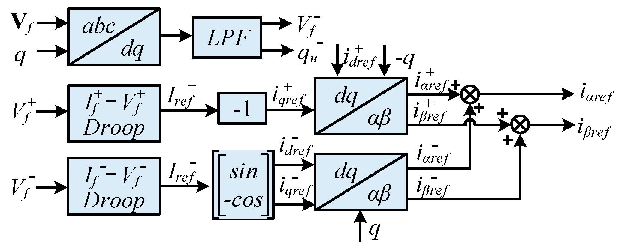
4.4. Structure of Current Reference Generator

During grid voltage sag faults, the corresponding positive and negative sequence current commands If+ and If can be derived using the current reference generation strategy mentioned above. As illustrated in Figure 18, both the current vectors If+ and If rotate at an angular velocity of ω but in opposite directions. The phase and angular frequency information for the positive sequence dq axis system are provided by the DSOGI-PLL, while the phase of the negative sequence coordinate system is opposite to that of the positive sequence coordinate system. In the dq axis system, the reference current values idref+, iqref+,idref, and iqref for the positive and negative sequence dq axis are given as
{ i d r e f + = 0 i q r e f + = I f + i d r e f = I f sin φ u i q r e f = I f cos φ u
where ju is the initial angle of the vector Vf in negative sequence dq axis. Then, the four current references are converted into the values in the ab axis to obtain iaref and ibref. Thus, the structure of the current reference generator is shown in Figure 19.

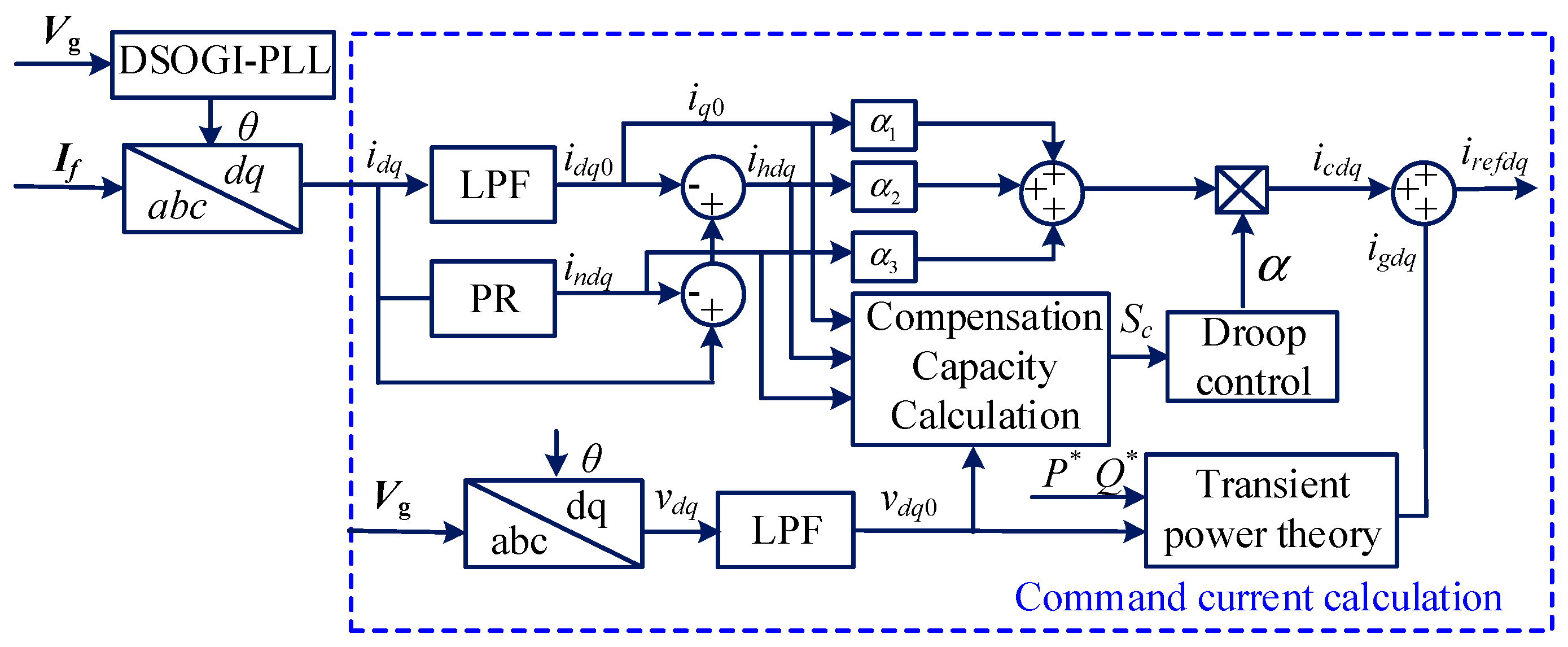
5. Enhanced Power Quality Control

To enhance the power quality in distributed networks with multiple converters, the analytic hierarchy process (AHP) and the coefficient of variation (CV) method are employed to evaluate the power quality in this section. Then, a weighted averaging method is proposed to inject the compensation current. In this manner, the balance between minimal capacity and optimal power quality can be guaranteed in a multi-converter system.

5.1. Injected Current Calculation

Since the inverter has a dual role in integrating DGs and managing power quality, the command current irefdq consists of the grid-connected current igdq and the compensation current icdq. Traditional converters use PQ control to achieve a stable power grid connection. Based on the theory of instantaneous power, igdq can be expressed as
[ i g d i g q ] = 1 u d 0 2 + u q 0 2 [ P * Q * Q * P * ] [ u d 0 u q 0 ]
To calculate icdq, the phase information of the PCC voltage is first obtained using the DSOGI-PLL, as shown in Figure 20, which ensures accurate and robust phase detection even under grid imbalance and harmonic distortion conditions. Following the Park transformation, the fundamental component idq0 and the negative sequence component indq of idq are distinguished as the direct and double-frequency terms, respectively. Then, a low-pass filter (LPF) and a second-order notch filter can be employed to effectively isolate them. Furthermore, by subtracting idq0 and indq from idq, the harmonic component ihdq can be extracted. Due to the limitation of the remaining capacity, each component is multiplied by the evaluation factors α1, α2 and α3 to achieve optimal management. Subsequently, the compensation factor α, derived from the droop curve, is applied to determine the final icdq. Therefore, the selection of the assessment and compensation factors is crucial for the effectiveness of the system.

5.2. Compensation Current Analysis

As illustrated in Figure 21, this paper proposes a comprehensive assessment method integrating the AHP and CV approaches. AHP is based on the subjective experience of decision-makers and can meet the actual needs of the electricity user side. The CV method is based on actual data, which makes the evaluation results objective. Finally, the weighted average method is used to combine the subjective and objective coefficients to obtain the final evaluation factor. The specific steps are as follows.
Firstly, it is necessary to establish an assessment model for power quality. Each inductor in the hierarchy shown in Figure 22 they are compared with each other to construct the importance matrix M as
M = A 1 A 2 A 3 | μ 11 μ 12 μ 13 μ 21 μ 22 μ 23 μ 31 μ 32 μ 33 |   A 1         A 2         A 3
where
μ i j = { 1 ,   equally   important 3 ,   moderately   important 5 ,   very   important reciprocal ,   represents   the   degree   of   unimportance
Since the matrix is derived from subjective judgments, a consistency check is required to verify its rationality. The consistency index (CI) is calculated as
C I = λ max n n 1
where λmax represents the maximum eigenvalue of the judgment matrix M and n is the number of the inductors.
Then, the consistency ratio (CR) is calculated as
C R = C I R I
where RI is the random index that is related to n, and it can be obtained from a standard RI table. Only if CR < 0.1 the consistency of the importance matrix is acceptable, indicating logical and reasonable evaluations. Finally, the subjective weights can be expressed as
β i = j = 1 3 μ i j 3 / i = 1 3 j = 1 3 μ i j 3
where βi represents the corresponding weight of elements in the indicator layer.
Using the CV method can help identify which parameters fluctuate more and may have a greater impact on power quality. It is the ratio of the standard deviation to the mean, allowing indicators of different units to be compared on the same scale. Firstly, the array of indicators is defined as Yj = [y1j,y2j,y3j], where y1j, y2j, and y3j represent the reactive, harmonic and negative sequence currents, respectively.
y i j = { 1 k + max | Y i | + y i j     positive - oriented   inductor y i j   negative - oriented   inductor
where yij represents the jth indicator of the ith period and a total of n periods of data are sampled. Meanwhile, all selected indicators are negative-oriented, meaning that a smaller value indicates a better condition.
Then Vi can be calculated as
V i = s i / y i ¯ = 1 n i = 1 n ( y i j y i j ¯ ) 2 / y i ¯
where
y j ¯ = 1 n i = 1 n y i j
Thus, the objective weights can be expressed as
γ i = V i / j = 1 3 V i
A higher CV indicates lower reliability of the data-driven results, and thus, more subjective weight needs to be added to the evaluation. The process of the weighted average is given as
τ i = β i γ i β 1 γ 1 + β 2 γ 2 + β 3 γ 3
The final evaluation factor is related to the compensation capacity required to solve various power quality problems and is expressed as
α i = τ i S j τ 1 S q + τ 2 S h + τ 3 S n   ( j = q , h , n )
where Sq, Sh, and Sn represent the required capacities for reactive, harmonic and unbalanced issues, respectively.
Ideally, the PLL is correctly locked to the frequency and the phase of the PCC voltage, then the resulting voltage at the q-axis will be close to zero. Thus, the total required compensation capacity is simplified as
S c = S q 2 + S h 2 + S n 2 =   3 U d 2 I q 0 2 + ( U d 2 I h d 2 + U d 2 I h q 2 ) + ( U d 2 I n d 2 + U d 2 I n q 2 )
The compensation factor α and Sc satisfy the droop curve shown in Figure 23, and their relationship can be expressed as
α = { 1       S c S c 0 1 k ( S c S c 0 ) S c > S c 0  
where Scmax indicates the equipment limit of the compensator; Sc0 is related to the minimum required compensation capacity.

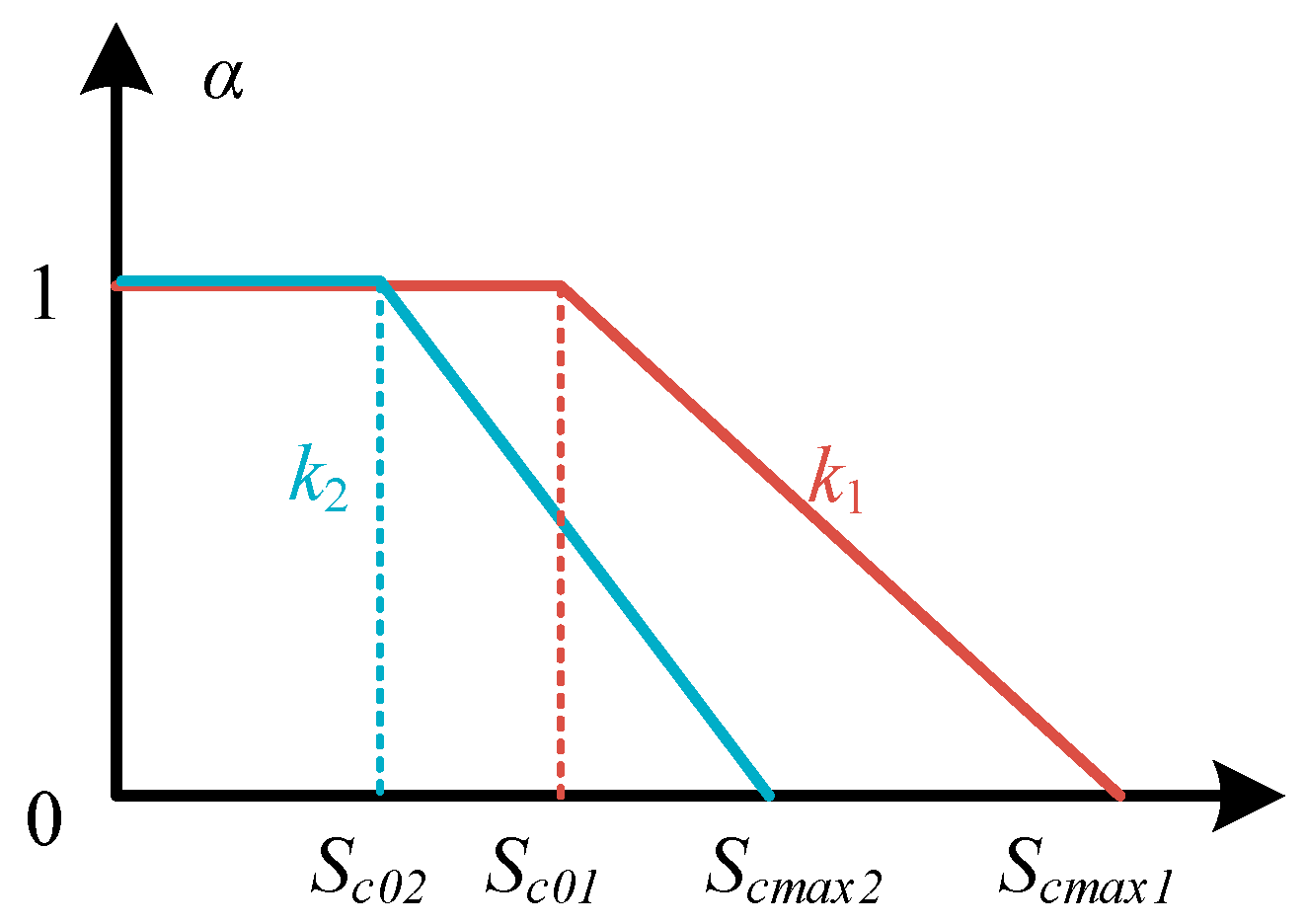
5.3. Controller Design

Typically, in the synchronous rotating dq reference frame, a PI controller can be employed to track commands at zero steady-state error. A multi-resonant PR controller is integrated to control a broader range of harmonic frequencies. As depicted in Figure 24, the controller is expressed as
G c ( s ) = K p + K i s + h = 2 , 6 , 12 , 18 2 K r h ω c h s s 2 + 2 ω c h s + ω h 2
where Kp, Ki and Kr are the proportional and integral gains of the PI and PR controller; ωh and ωc are the angular frequencies of the hth harmonic and the filter cutoff frequency. Since harmonic currents in the power grid-primarily originate from nonlinear loads, the harmonic frequency on the dq axis is 6k times the fundamental frequency (k = 1, 2, 3, …) after Fourier expansion. In addition, the frequency of the negative sequence current is twice the fundamental frequency after transformation. Hence, h is mainly composed of frequencies 2, 6, 12 and 18.

6. Simulation Validation

To validate the effectiveness of the proposed scheme, several simulations are conducted in MATLAB/Simulink environment and a multi-core CPU with 32 GB RAM, which aims to enhance the clarity and replicability of the simulation. The key parameters are listed in Table 2 and Table 3. Firstly, the stability boundary of the GFM converter is validated. Then, the voltage support capacity of the GFL converter during symmetrical faults and asymmetrical faults is tested. Finally, the proposed power quality improvement method is tested in a multi-converter system.

6.1. Stability Boundary Test of GFM Converter

According to Table 1, the GFM converter was configured with parameters within the stability boundary range of (0.04, 255). Experiments were conducted at SCR values of 2 and 4 while keeping the control parameters unchanged. The waveforms of the capacitor voltage Uf and the grid-side current Ig are shown in Figure 25 and Figure 26. It can be seen that the designed inner loop control parameters successfully maintained system stability across the tested SCR range, demonstrating strong robustness.
To further verify the accuracy of the proposed inner loop parameter stability boundaries, experiments were conducted using a stable boundary point (0.04, 255) and an unstable boundary point (0.14, 500) as case studies, as shown in Figure 27. At time t1, the control parameters were switched from (0.04, 255) to (0.14, 500), resulting in oscillations in the capacitor voltage Uf of the GFM converter, which confirms the effectiveness of the designed inner loop control parameter boundaries.

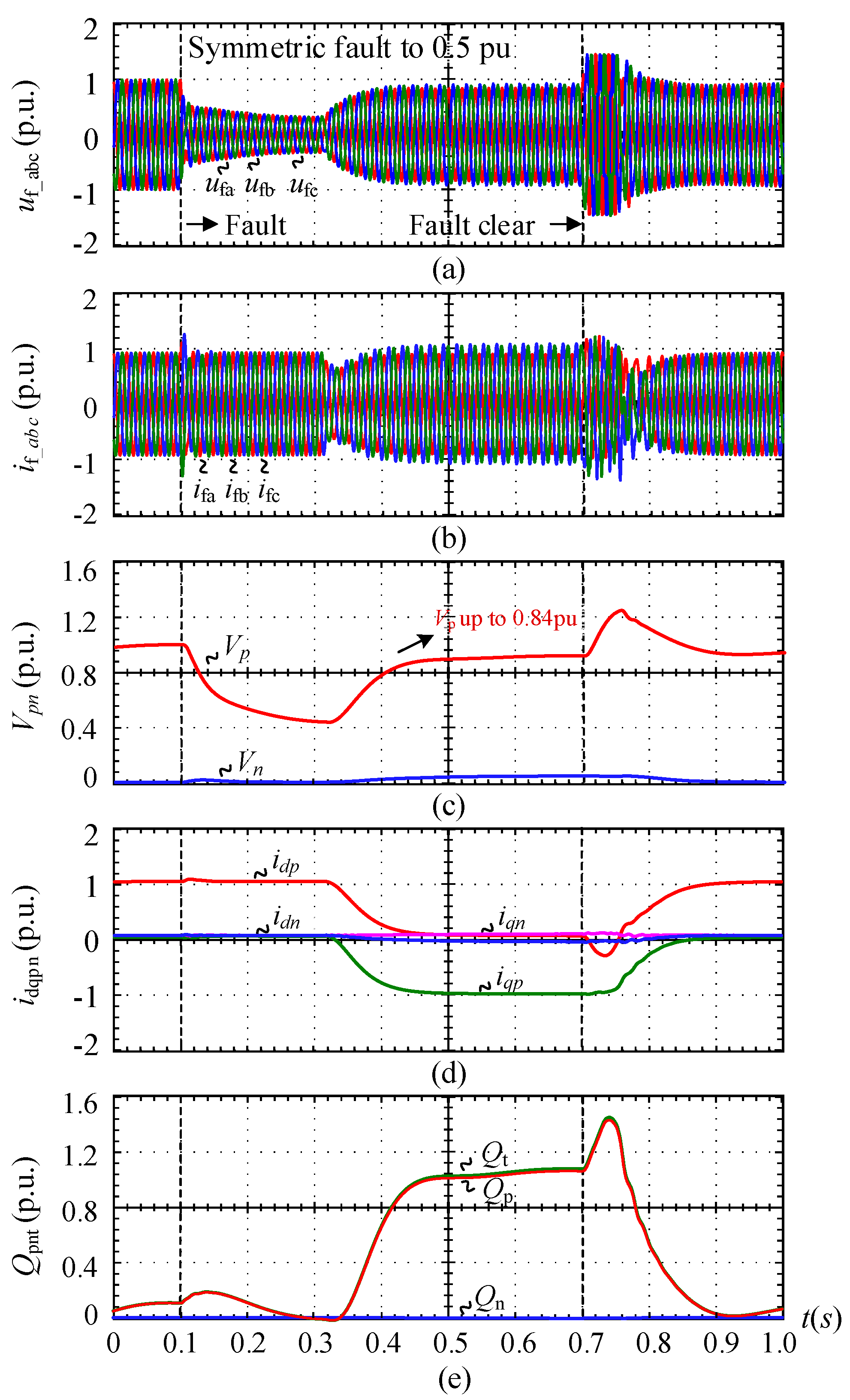
6.2. Symmetrical Grid Faults Test of GFL Converter

This case is conducted to test the PCC voltage support capability under symmetrical faults. Before the occurrence of a fault, the GFL converter delivers a rated active power of 1.0 p.u. to the grid. At 0.1 s, the grid experiences a voltage sag fault. The GFL converter responds to the grid fault 100 ms later by injecting the maximum positive and negative sequence reactive power into the grid. At 0.7 s, the grid voltage returns to normal; the variation process of the PCC voltage before and after the symmetrical fault is shown in Figure 28a. Figure 28b illustrates the waveform of the converter’s three-phase currents before and after the fault. Figure 28c displays the changes in the positive and negative sequence components of the PCC voltage before and after the fault. Figure 28d presents the variation of the positive and negative sequence dq currents before and after the fault. Figure 28e shows the change in the converter’s reactive current before and after the fault. During the symmetrical voltage sag of the grid to 0.5 p.u., the converter injects 1.2 p.u. of possible sequence reactive power into the grid, as shown in Figure 28e. This maximizes the support of the PCC voltage to 0.84 p.u. at the same time, injecting a positive sequence reactive current of 1.0 p.u. into the grid, as shown in Figure 28b,c, which reaches the boundary of the converter’s capacity constraint.

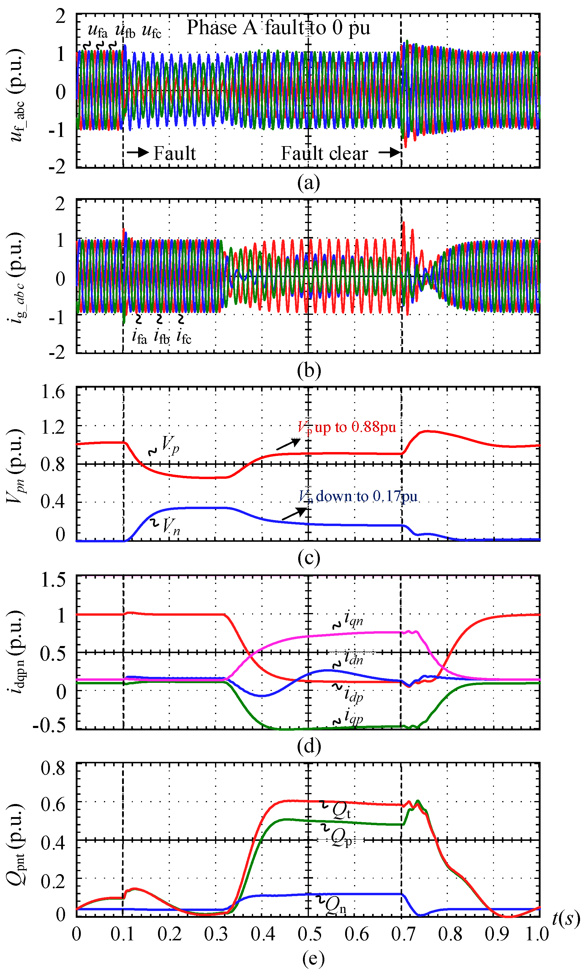
6.3. Asymmetrical Grid Faults Test of GFL Converter

In this case, an asymmetric fault is simulated to verify the PCC voltage support capability. Figure 29a shows the variation process of the PCC voltage before and after the symmetrical fault. Figure 29b illustrates the waveform of the converter’s three-phase currents before and after the fault. Figure 29c displays the changes in the positive and negative sequence components of the PCC voltage before and after the fault. Figure 29d presents the variation of the positive and negative sequence dq currents before and after the fault. Figure 29e shows the change in the converter’s reactive current before and after the fault. As illustrated in Figure 29a, when the grid voltage of phase A experiences a short circuit to zero, the positive sequence component of the PCC voltage drops to 0.67 p.u., concurrently generating a negative sequence voltage of 0.33 p.u. At 0.2 s, the converter responds to the asymmetrical fault by injecting −0.65 p.u. of positive sequence reactive current and 0.65 p.u. of negative sequence reactive current into the grid. This action elevates the positive sequence component of the PCC voltage to 0.88 p.u. at the same time, reducing the negative sequence component to 0.17 p.u. At this point, the converter injects a total reactive power of 0.73 p.u. into the grid, comprising 0.61 p.u. of positive sequence reactive power and 0.12 p.u. of negative sequence reactive power. The converter does not inject its full capacity of reactive power because the asymmetrical nature of the three-phase currents, resulting from the phase A to ground short circuit, causes the phase A current to exceed the currents of phases B and C significantly. Consequently, the converter is constrained by its maximum current limit, preventing it from outputting the rated capacity of reactive current. This test result is consistent with the theoretical analysis presented earlier.

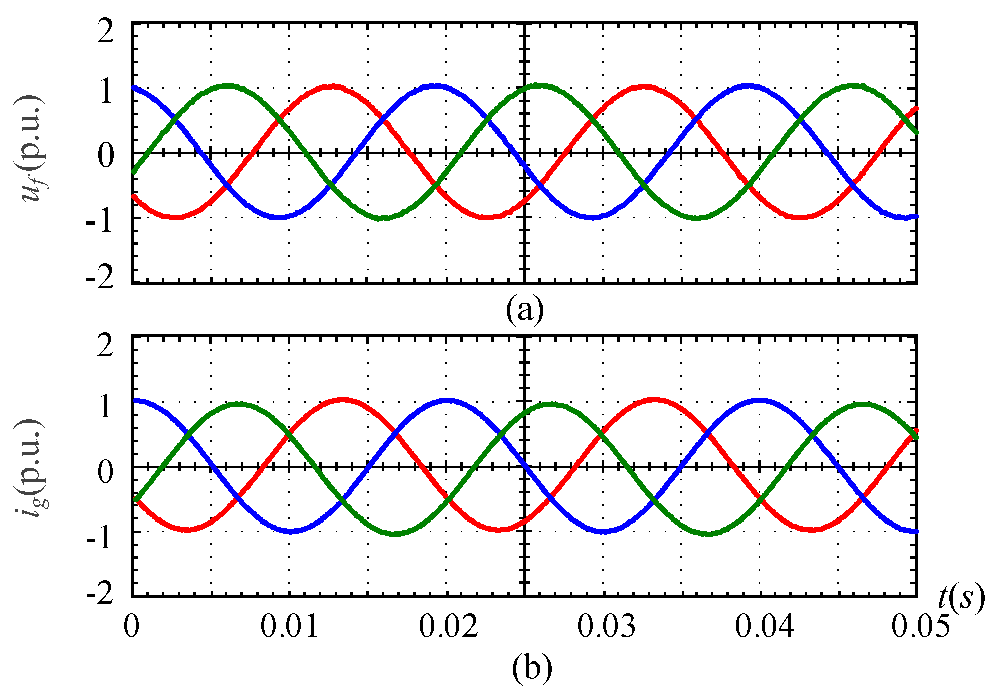
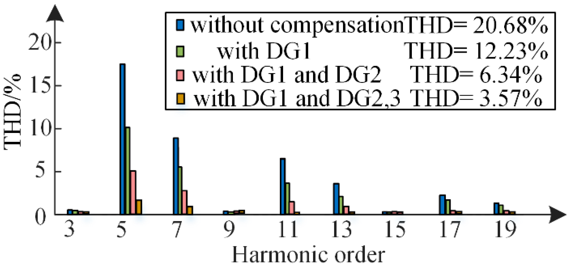
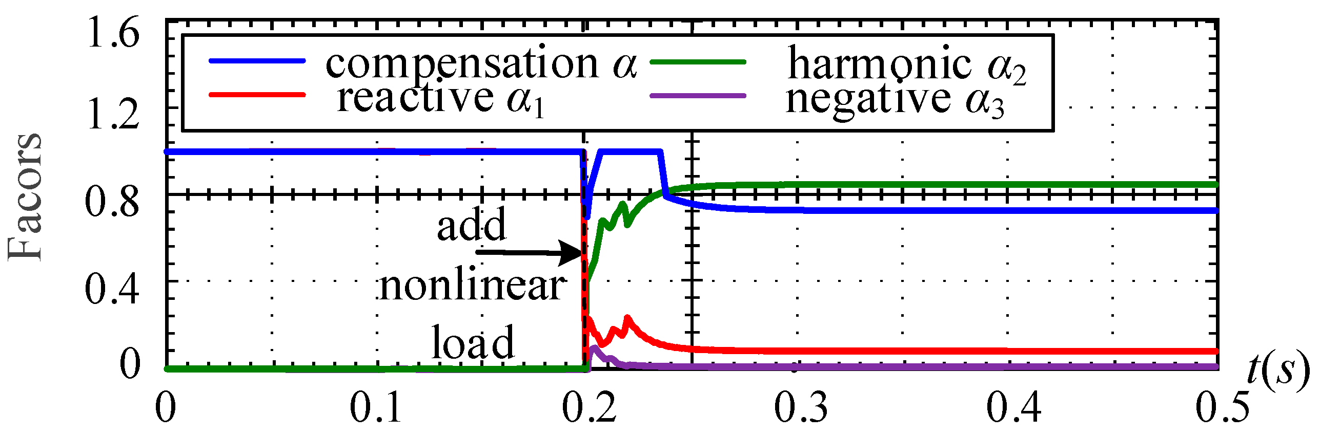
6.4. Cooperative Management of Multi-Converters

In a three-DG system, the nonlinear load is added at 0.2 s. Figure 30 illustrates that the grid current igabc predominantly contains 5th, 7th, and 11th harmonics, resulting in an initial total harmonic distortion (THD) of 20.68%. Because DG1 is closer to the load, the compensation is started first, as shown in Figure 31. However, its limited capacity restricts full harmonic compensation, reducing THD to 12.23%, which is inadequate. At 0.5 s, DG2 engages in the compensation, as depicted in Figure 32. The collaborative management of DG1 and DG2 significantly only lowers THD to 6.36%. At 0.7 s, the reactive load is added. Since the reactive coefficient has the greatest weight, the reactive power coefficient rises suddenly, as shown in Figure 32. In order to better manage the current, at 0.5 s, DG3 engages in the compensation, reducing THD to 3.57%, with each odd harmonic below 5%, aligning with national standards. Finally, at 1.2 s, the unbalanced load is added. Since the unbalanced current has the lowest weight, it can be seen from Figure 33 that it has little effect on other coefficients. More importantly, the droop curve entirely depends on equipment capacity, ensuring that DGs do not interfere with each other, thus maintaining the stability of the electrical system.

7. Conclusions

In this paper, the stability-oriented design of controller parameters and power quality improvement method for the distribution network is proposed. Firstly, the model of the grid forming and grid following converters are established. Then, a D-Partition-based inner loop parameters design method is proposed for grid forming converters to make its stability meet phase margin, gain margin, and short circuit ratio. Meanwhile, an adaptive positive and negative sequence reactive current command generation strategy is developed to realize voltage support capacity enhancement during symmetrical and asymmetrical faults, which can increase the PCC voltage by up to 0.3 p.u. within the converter capacity limit, thereby assisting in the restoration of a grid fault. Moreover, an enhanced power quality control strategy is proposed based on the AHP and CV methods. This approach not only considers subjective and objective factors but also combines the capacity limitations of the equipment. In this manner, a precise determination of the compensation task prioritization and resource allocation can be achieved, which decreases the THD from 20% to less than 5% to effectively enhance the power quality. The application of the proposed method ensures the plug-and-play of distributed generators and the system’s good power quality. Finally, the effectiveness of the proposed method is verified by simulations.

Author Contributions

Conceptualization, M.Z. and T.S.; methodology, M.Z.; software, M.Z.; validation, M.Z., Y.L. and S.G.; formal analysis, Z.X.; investigation, R.F.; resources, T.S. and X.X.; data curation, T.S.; writing—original draft preparation, M.Z.; writing—review and editing, T.S. and X.X.; visualization, T.S.; supervision, T.S.; project administration, M.Z. and T.S.; funding acquisition, X.X. All authors have read and agreed to the published version of the manuscript.

Funding

This research was funded by State Grid Shanxi Electric Power Company Science and Technology Project Research (52053023001L).

Data Availability Statement

The original contributions presented in the study are included in the article, further inquiries can be directed to the corresponding author.

Conflicts of Interest

The authors declare no conflicts of interest.

References

  1. Liu, T.; Wang, X.; Liu, F.; Xin, K.; Liu, Y. A current limiting method for single-loop voltage-magnitude controlled grid-forming converters during symmetrical faults. IEEE Trans. Power Electron. 2022, 37, 4751–4763. [Google Scholar] [CrossRef]
  2. Shen, C.; Shuai, Z.; Shen, Y.; Peng, Y.; Liu, X.; Li, Z.; Shen, Z. Transient stability and current injection design of paralleled current-controlled vscs and virtual synchronous generators. IEEE Trans. Smart Grid 2021, 12, 1118–1134. [Google Scholar] [CrossRef]
  3. Rosso, R.; Wang, X.; Liserre, M.; Lu, X.; Engelken, S. Grid-forming converters: Control approaches, grid synchronization, and future trends–A review. IEEE Open J. Ind. Appl. 2021, 2, 93–109. [Google Scholar] [CrossRef]
  4. Afshari, A.; Davari, M.; Karrari, M.; Gao, W.; Blaabjerg, F. A multivariable, adaptive, robust, primary control enforcing predetermined dynamics of interest in islanded microgrids based on grid-forming inverter-based resources. IEEE Trans. Automat. Sci. Eng. 2024, 21, 2494–2506. [Google Scholar] [CrossRef]
  5. Brito, M.A.G.D.; Galotto, L., Jr.; Sampaio, L.P.; Melo, G.D.A.E.; Canesin, G.A. Evaluation of the main MPPT techniques for photovoltaic applications. IEEE Trans. Ind. Electron. 2013, 60, 1156–1167. [Google Scholar] [CrossRef]
  6. Zarei, S.F.; Mokhtari, H.; Ghasemi, M.A.; Peyghami, S.; Davari, P.; Blaabjerg, F. Control of grid-following inverters under unbalanced grid conditions. IEEE Trans. Energy Convers. 2020, 35, 184–192. [Google Scholar] [CrossRef]
  7. Tang, Y.; Loh, P.C.; Wang, P.; Choo, F.H.; Gao, F.; Blaabjerg, F. Generalized design of high-performance shunt active power filter with output LCL filter. IEEE Trans. Ind. Electron. 2012, 59, 1443–1452. [Google Scholar] [CrossRef]
  8. Zhang, S.; Qiao, W.; Qu, L.; Wang, J. Analysis and synchronization controller design of dual-port grid-forming voltage-source converters for different operation modes. iEnergy 2024, 3, 46–58. [Google Scholar] [CrossRef]
  9. Dannehl, J.; Wessels, C.; Fuchs, F.W. Limitations of voltage-oriented PI current control of grid-connected PWM rectifiers with LCL filters. IEEE Trans. Ind. Electron. 2009, 56, 380–388. [Google Scholar] [CrossRef]
  10. Twining, E.; Holmes, D.G. Grid current regulation of a three-phase voltage source inverter with an LCL input filter. IEEE Trans. Power Electron. 2003, 18, 888–895. [Google Scholar] [CrossRef]
  11. Zhang, X.; Yu, C.; Liu, F.; Li, F.; Xu, H. Overview on resonance characteristics and resonance suppression strategy of multi-parallel photovoltaic inverters. Chin. J. Elect. Eng. 2016, 2, 40–51. [Google Scholar]
  12. Hušek, P. Decentralized PI controller design based on phase margin specifications. IEEE Trans. Control Syst. Technol. 2014, 22, 346–351. [Google Scholar] [CrossRef]
  13. Hasan, S.; Agarwal, V. A voltage support scheme for distributed generation with minimal phase current under asymmetrical grid faults. IEEE Trans. Ind. Electron. 2023, 70, 10261–10270. [Google Scholar] [CrossRef]
  14. Zhao, C.; Sun, D.; Duan, X.; Nian, H. Current reference optimization for inverter-based resources to mitigate grid voltage vnbalance factor. IEEE Trans. Power Syst. 2024, 39, 6103–6106. [Google Scholar] [CrossRef]
  15. Lee, C.T.; Hsu, C.W.; Cheng, P.T. A low-voltage ride-through technique for grid-connected converters of distributed energy resources. IEEE Trans. Ind. Appl. 2011, 47, 1821–1832. [Google Scholar] [CrossRef]
  16. López, M.A.G.; de Vicuña, J.L.G.; Miret, J.; Castilla, M.; Guzmán, R. Control strategy for grid-connected three-phase inverters during voltage sags to meet grid codes and to maximize power delivery capability. IEEE Trans. Power Electron. 2018, 33, 9360–9374. [Google Scholar] [CrossRef]
  17. Pleshakova, E.; Osipov, A.; Gataullin, S.; Gataullin, T.; Vasilakos, A. Next gen cybersecurity paradigm towards artificial general intelligence: Russian market challenges and future global technological trends. J. Comput. Virol. Hack. Tech. 2024, 20, 429–440. [Google Scholar] [CrossRef]
  18. Zhao, X.; Bian, D. Currents’-physical-component-based reactive power compensation optimization in three-phase, four-wire systems. Appl. Sci. 2024, 14, 5043. [Google Scholar] [CrossRef]
  19. Zelenina, A.; Petrosov, D.; Pleshakova, E.; Osipov, A.; Ivanov, M.N.; Choporov, O.; Preobrazhenskiy, Y.; Petrsova, N.; Roga, S.; Lopatnuk, L.; et al. Modeling of management processes in distributed organizational systems. Proc. Comput. Sci. 2022, 213, 377–384. [Google Scholar] [CrossRef]
  20. Mousavi, S.Y.M.; Jalilian, A.; Savaghebi, M.; Guerrero, J.M. Coordinated control of multifunctional inverters for voltage support and harmonic compensation in a grid-connected microgrid. Electr. Power Syst. Res. 2018, 155, 254–264. [Google Scholar] [CrossRef]
  21. Wang, L.; Zhang, D.; Wang, Y.; Wu, B.; Athab, H.S. Power and voltage balance control of a novel three-phase solid-state transformer using multilevel cascaded H-bridge inverters for microgrid applications. IEEE Trans. Power Electron. 2016, 31, 3289–3301. [Google Scholar] [CrossRef]
  22. Gataullin, T.M.; Gataullin, S.T. Best economic approaches under conditions of uncertainty. In Proceedings of the 2018 Eleventh International Conference on Management of Large-Scale System Development (MLSD), Moscow, Russia, 1–3 October 2018. [Google Scholar]
  23. Sharma, A.; Rajpurohit, B.S.; Singh, S.N. A review on economics of power quality: Impact, assessment and mitigation. Renew. Sustain. Energy Rev. 2018, 88, 363–372. [Google Scholar] [CrossRef]
  24. Sun, H.; Lin, X.; Chen, S.; Ji, X.; Liu, D.; Jiang, K. Transient stability analysis of the standalone solar-storage AC supply system based on grid-forming and grid-following converters during sudden load variation. IET Renew. Power Gener. 2022, 17, 1286–1302. [Google Scholar] [CrossRef]
  25. Shao, W.; Wu, R.; Ran, L.; Jiang, H.; Mawby, P.A.; Rogers, D.J.; Green, T.C.; Coombs, T.; Yardley, K.; Kastha, D.; et al. Apower module for grid inverter with in-built short-circuit fault current capability. IEEE Trans. Power Electron. 2020, 35, 10567–10579. [Google Scholar] [CrossRef]
  26. Qoria, T.; Gruson, F.; Colas, F.; Denis, G.; Prevost, T.; Guillaud, X. Critical clearing time determination and enhancement of grid-forming converters embedding virtual impedance as current limitation algorithm. IEEE J. Emerg. Sel. Topics Power Electron. 2020, 8, 1050–1061. [Google Scholar] [CrossRef]
  27. Lei, J.; Xiang, X.; Liu, B.; Li, W.; He, X. Transient stability analysis of grid forming converters based on damping energy visualization and geometry approximation. IEEE Trans. Ind. Electron. 2024, 71, 2510–2521. [Google Scholar] [CrossRef]
  28. Sun, J. Impedance-Based Stability Criterion for Grid-Connected Inverters. IEEE Trans. Power Electron. 2011, 26, 3075–3078. [Google Scholar] [CrossRef]
  29. Xie, Z.; Wu, W.; Chen, Y.; Gong, W. Admittance-based stability comparative analysis of grid-connected inverters with direct power control and closed-loop current control. IEEE Trans. Ind. Electron. 2021, 66, 8333–8344. [Google Scholar] [CrossRef]
  30. Zhou, L.; Wu, W.; Chen, Y.; He, Z.; Zhou, X.; Huang, X.; Yang, L.; Luo, A.; Guerrero, J.M. Virtual positive-damping reshaped impedance stability control method for the offshore MVDC system. IEEE Trans. Power Electron. 2019, 34, 4951–4966. [Google Scholar] [CrossRef]
  31. Zhang, X.; Zhong, Q.-C.; Ming, W. Stabilization of cascaded dc/dc converters via adaptive series-virtual-impedance control of the load converter. IEEE Trans. Power Electron. 2016, 31, 6057–6063. [Google Scholar] [CrossRef]
  32. Jalili, K.; Bernet, S. Design of LCL filters of active-front-end two-level voltage-source converters. IEEE Trans. Ind. Electron. 2009, 56, 1674–1689. [Google Scholar] [CrossRef]
  33. Qu, Z.; Peng, J.C.-H.; Yang, H.; Srinivasan, D. Modeling and analysis of inner controls effects on damping and synchronizing torque components in VSG-controlled converter. IEEE Trans. Energy Convers. 2021, 36, 488–499. [Google Scholar] [CrossRef]
  34. Lanzkron, R.; Higgins, T. D-decomposition analysis of automatic control systems. IRE Trans. Autom. Control 1959, 4, 150–171. [Google Scholar] [CrossRef]
  35. Li, M.; Zhang, X.; Guo, Z.; Pan, H.; Ma, M.; Zhao, W. Impedance adaptive dual-mode control of grid-connected inverters with large fluctuation of SCR and its stability analysis based on D-Partition method. IEEE Trans. Power Electron. 2021, 36, 14420–14435. [Google Scholar] [CrossRef]
Figure 1. A typical structure of a grid-connected power conversion system.
Energies 17 06215 g001
Figure 2. Main circuit and control structure of a GFM converter.
Energies 17 06215 g002
Figure 3. Main circuit and control structure of a GFL converter.
Energies 17 06215 g003
Figure 4. Block Diagram of Droop Control Strategy.
Energies 17 06215 g004
Figure 5. Block Diagram of VSG Control Strategy.
Energies 17 06215 g005
Figure 6. Block Diagram of VOC Control Strategy.
Energies 17 06215 g006
Figure 7. Voltage dynamics for the GFM converter.
Energies 17 06215 g007
Figure 8. Vector diagram of PCC voltage, current, and grid voltage.
Energies 17 06215 g008
Figure 9. A typical relationship diagram of the current vector on the injection side, the voltage vector of the grid, and the voltage vector on the PCC.
Energies 17 06215 g009
Figure 10. Block diagram of a unity feedback system with a PI controller.
Energies 17 06215 g010
Figure 11. Controller block diagram including phase gain margin tester.
Energies 17 06215 g011
Figure 12. The feasible region for inner loop parameters is optimized with PM and GM constraints.
Energies 17 06215 g012
Figure 13. The Bode diagram of the open-loop transfer function with PI parameters set to (0.0322,334).
Energies 17 06215 g013
Figure 14. Feasible region for inner loop parameters optimized with SCR constraints.
Energies 17 06215 g014
Figure 15. The Bode diagram of the output impedance of the GFM converter with PI set to (0.05, 250).
Energies 17 06215 g015
Figure 16. Droop curves of positive and negative sequence components of PCC voltage with positive and negative sequence reactive currents.
Energies 17 06215 g016
Figure 17. Feasible region of (Vd+, Vu).
Energies 17 06215 g017
Figure 18. Voltage and current vector diagram at PCC for symmetric and asymmetric faults.
Energies 17 06215 g018
Figure 19. Control diagram of the positive-sequence and negative-sequence reference current generator.
Energies 17 06215 g019
Figure 20. Process of command current calculation.
Energies 17 06215 g020
Figure 21. Calculation process of comprehensive weight.
Energies 17 06215 g021
Figure 22. Evaluation index system for power quality.
Energies 17 06215 g022
Figure 23. Droop curves of α with compensation capacity.
Energies 17 06215 g023
Figure 24. The current tracking strategy uses PI and multi-resonant PR control.
Energies 17 06215 g024
Figure 25. Experimental Waveforms for SCR Values of 2.
Energies 17 06215 g025
Figure 26. Experimental Waveforms for SCR Values of 4.
Energies 17 06215 g026
Figure 27. Experimental Waveforms Under Control Parameter Switching.
Energies 17 06215 g027
Figure 28. Simulation results under symmetrical faults.
Energies 17 06215 g028
Figure 29. Simulation results under asymmetrical faults.
Energies 17 06215 g029
Figure 30. FFT analysis of grid-connected currents.
Energies 17 06215 g030
Figure 31. The assessment and compensation factors of DG1.
Energies 17 06215 g031
Figure 32. The assessment and compensation factors of DG2.
Energies 17 06215 g032
Figure 33. The assessment and compensation factors of DG3.
Energies 17 06215 g033
Table 1. Summary of GFM control technology characteristics.
Performance AreaDroop ControlVSGVOC
Inertia SupportNonePresentPresent
Response SpeedFastSlowFast
Current SharingModerateModerateGood
Output OscillationNonePresentPresent
Power RegulationAvailableAvailableAvailable
Table 2. System and control parameter of GFM.
ParametersValueParametersValue
Grid voltage ugN380 VConverter-side inductance Lm1.6 mH
Rated angular frequency ω050 HzFilter capacitance Cm20 μF
Switching frequency16 kHzPassive damping resistance Rm0.5 Ω
Table 3. System and control parameter of GFL.
ParametersValueParametersValue
Nominal Power150 kVADC-bus capacitor Cbus375 μF
AC frequency fac50 HzSwitch frequency20 kHz
Filter inductance Lf100 μHLine inductance Lg3 mH
Disclaimer/Publisher’s Note: The statements, opinions and data contained in all publications are solely those of the individual author(s) and contributor(s) and not of MDPI and/or the editor(s). MDPI and/or the editor(s) disclaim responsibility for any injury to people or property resulting from any ideas, methods, instructions or products referred to in the content.

