Experimental Investigation of Wall Confluent Jets on Transparent Large-Space Building Envelopes: Part 1—Application in Heating Greenhouses

Abstract

Insulating building envelopes is crucial for maintaining indoor thermal comfort, particularly in large-space enclosures like greenhouses having transparent envelopes. Transparent envelopes allow natural light but challenge temperature regulation due to their low thermal mass and high U-values, which enable significant heat transfer between indoor and outdoor environments. This field study aims to experimentally investigate whether warm wall confluent jets (WCJs) can maintain the required indoor climate conditions in a greenhouse exposed to dynamic meteorological conditions in winter. It analyzed the impact of the airflow rate, number of nozzle rows, and room air temperature setpoint on WCJ heating performance on the ceiling, external wall, and room air. Measurements were performed with thermocouples and constant current anemometers, and the response surface methodology evaluated the effect of design variables on WCJ flow, thermal behavior, and the indoor environment. The results show that WCJs provided recommended air velocities and temperatures indoors, with the airflow rate having the strongest effect on flow and thermal behavior, while the number of nozzle rows had a moderate effect. This study developed response surface models related to room air temperature, ceiling surface temperature, external wall temperature, and supply air temperature. Supply temperatures between 27 °C and 40 °C suggest using low-exergy heat sources, like industrial waste heat, to sustain greenhouse operations during winter.

1. Introduction

The building envelope, encompassing components such as foundations, roofs, walls, outside doors, and windows, serves as the protective barrier between indoor and outdoor environments [1,2]. Its design is influenced by factors like the size, purpose, and architectural aesthetics of the building. In large-space enclosures—such as railway stations, airport terminals [3,4], sports facilities [5], shopping centers [6], and greenhouses [7,8]—significant portions of the envelope often consist of transparent materials. These transparent elements, including expansive windows and skylights, allow natural light to enhance visual comfort, promote social interactions, and contribute to the building’s aesthetic appeal in modern architecture. For greenhouses specifically, transparent glass or plastic envelopes are essential to transmit the solar radiation and natural light necessary for crop growth [9,10].

However, transparent building envelopes present challenges in controlling heat transfer between indoor and outdoor environments, significantly affecting building energy performance [11,12,13]. Transparent materials typically have low thermal mass and high thermal transmittance (U-value), making indoor environments susceptible to temperature fluctuations due to weather changes in the outdoor environment. Low thermal mass reduces the building envelopes’ ability to store sensible or latent heat, adversely impacting building energy utilization, indoor temperatures, and occupant comfort [14,15,16].

Globally, the building sector uses about 40% of primary energy and contributes to approximately 36% of greenhouse gas emissions [17,18,19]. The heating, ventilation, and air conditioning (HVAC) systems represent a significant portion of this energy use, especially in large-space enclosures, where they can account for 40–80% of the total energy supply [20,21,22,23]. The energy use is even higher in cold regions, as heat loss through building envelopes alone accounts for approximately 40% of the total energy supplied by HVAC systems due to the significant temperature difference between indoor and outdoor environments [16,24].

Various strategies are employed to minimize heat transfer through building envelopes, including installing opaque or transparent insulation materials [25]. Insulation lowers the thermal transmittance of building envelopes [26], reducing energy costs [11,25], enhancing thermal climate [27], and protecting the building and its contents. It helps regulate indoor temperatures by minimizing heat loss in winter and heat gain in summer. These energy-saving measures are crucial for large-space enclosures with significant heating and cooling costs. Additionally, insulation prevents condensation by keeping surfaces warm and reducing moisture buildup, thereby avoiding mold and structural damage [28].

However, conventional opaque insulation is often unsuitable for some large-space enclosures because it interferes with aesthetics, visual comfort, and social interactions. In greenhouses, for example, opaque insulation would obstruct natural daylight, leading to increased use of artificial lighting and potentially poor crop growth. Despite this, greenhouses still require strategies to buffer against rapid temperature changes in the outdoor environment.

Greenhouses play a critical role in protected food production systems within the circular economy [29,30,31], aiding in a transition to more economic, ecological, and socially sustainable food production [32]. They provide optimally controlled environments to increase crop yield and ensure cost-effective production [33,34] in regions or under conditions where open-field agricultural practices are untenable. In Sweden, for example, greenhouses afford extended growing seasons in transition months but are shut down during winter due to high operational costs [35].

We propose a strategy that utilizes wall confluent jets (WCJs) for large-space enclosures with transparent building envelopes that neither obstruct natural light nor alter building aesthetics. Using the greenhouse as a case study, this study investigates the use of warm wall confluent jets (WCJs) to create a protective layer on the building’s transparent envelope, aiming to create optimal indoor air temperatures against transient meteorological conditions. Therefore, this study aims to test whether WCJs can maintain the required operational indoor climate conditions for greenhouses during winter by utilizing low-grade waste heat. This would allow the year-round operation of greenhouses, consequently increasing productivity, revenue generation, and food security.

A WCJ is a unified jet formed by confluent jets (CJs)—multiple circular air jets flowing in parallel and merging into a single air jet, which develops and attaches to the proximal wall as it moves downstream [36,37].

Confluent jets have applications in environmental engineering (e.g., pollution dispersion, wastewater treatment), meteorology, ventilation systems, combustion systems, and fluid dynamics research [38]. Research on confluent jets has focused on their behavior in the near field [39], particularly on the influence of array size, jet spacing, and intra-jet interactions and the flow fields [38,40]. Experimental and numerical studies have investigated the design and performance of confluent jet supply devices in various ventilation settings, including in classrooms [41,42], conference rooms, offices, and industrial spaces [38,43].

This study investigates the potential of using WCJs in greenhouses by optimizing the insulation properties of the boundary layer formed on the attached surface (building envelope) by delivering and controlling the required operational indoor environment. The layer acts as transparent insulation, isolating the indoor environment from the colder outdoor conditions while allowing sunlight to reach the crops. The wall-attaching flow behavior controls indoor air temperatures, and the heated supply jet prevents moisture condensation on the cold boundary surfaces. Figure 1 illustrates the characteristic velocity and temperature of a WCJ supplied with bulk velocity (U_b) and temperature (T_in) from a diffuser placed parallel and close to a vertical cold wall, propagating towards the floor. The velocity and temperature profiles vary across three major regions of the WCJ: the merging region, wall core zone, and impinging wall zone [43,44].

WCJs are suitable for spaces with complex geometry because they have lower entrainment rates, better energy performance, reduced velocity decay rates, and better momentum conservation [43,46,47]. Wall confluent jet ventilation (WCJV) systems create better indoor air quality and thermal comfort than mixing and displacement ventilation systems [44,48,49]. Due to their higher momentum, WCJs are less sensitive to obstructions, enabling them to penetrate deeper into indoor spaces [49]—a feature beneficial for larger areas like greenhouse applications.

In this study, we examine the potential application in a greenhouse by focusing on the influence of the number of nozzle rows (n) on the confluent jet diffuser, the supply airflow rate ($\dot{V}$), and the room air temperature setpoint (T_spt). We assess the performance and characteristics of the system on an inclined transparent plastic ceiling envelope and the external wall under heating mode conditions. The field studies are an extension of the laboratory experimental studies reported in [45]. This study explores the potential of WCJs as an innovative insulating mechanism for greenhouse envelopes. By utilizing low-grade waste heat, we seek to determine whether WCJs can maintain the required operational indoor climate conditions during winter, thereby improving energy efficiency without compromising the greenhouse’s functionality or aesthetics.

2. Materials and Methods

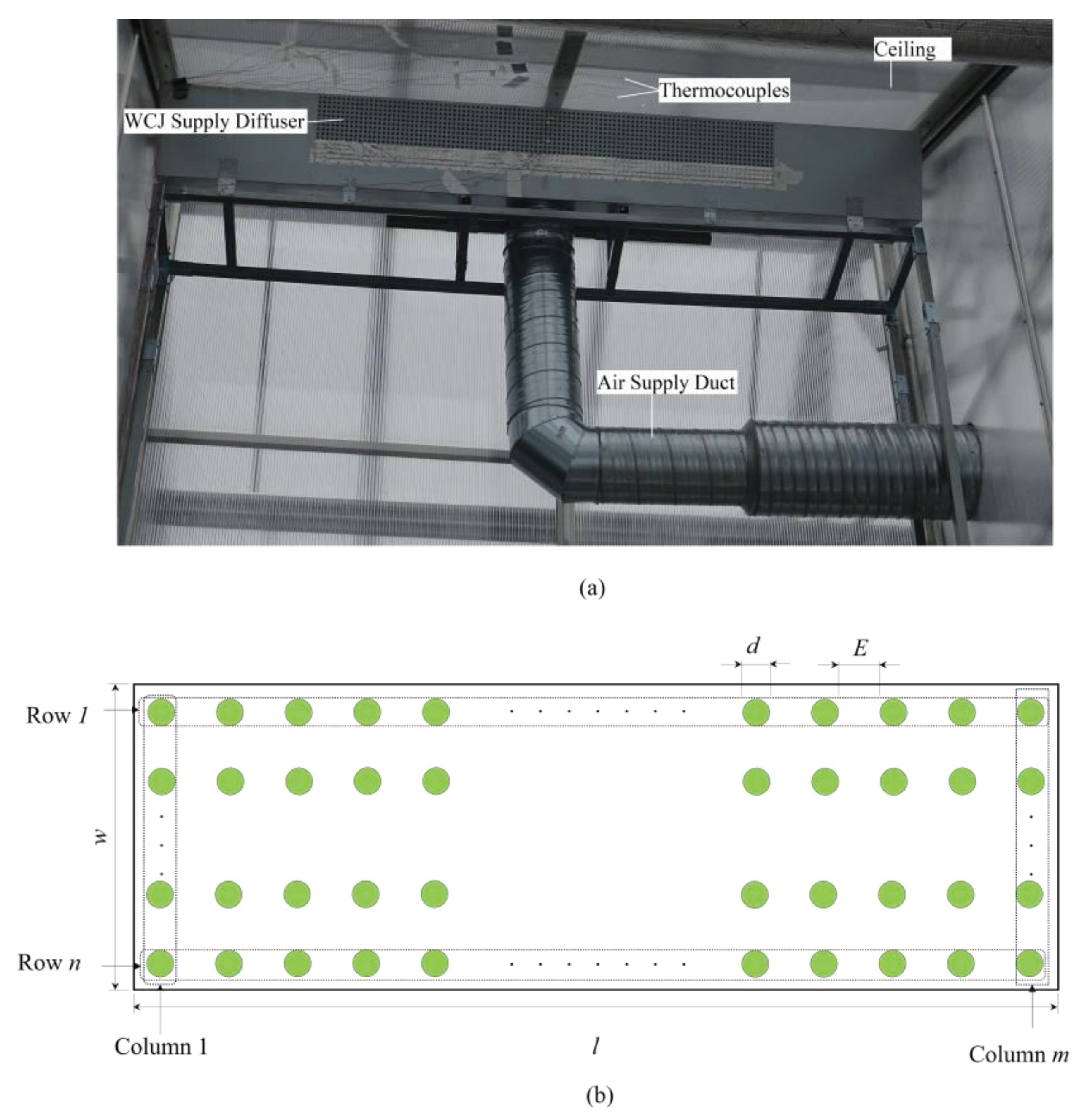
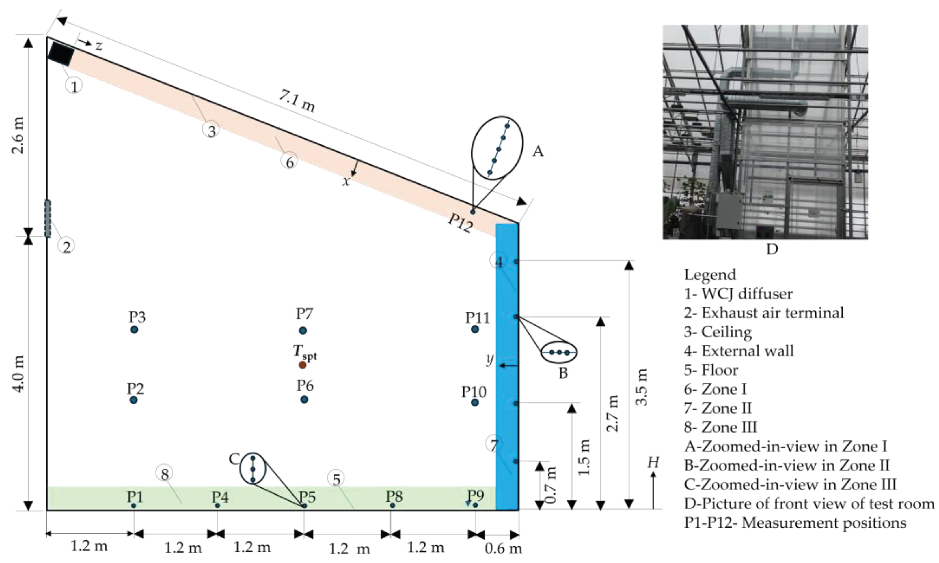
2.1. Research and Measurement Facility

This study was conducted in Hofors, a town in mid-Sweden, in a typical greenhouse. The test room was a partition with three side walls enclosed in the main greenhouse, while the roof and external wall were directly exposed to the outdoor environment with transient meteorological conditions. The field experiments were conducted in winter conditions from December 2023 to March 2024. According to the Swedish Meteorological and Hydrological Institute (SMHI), the average winter temperature in Sweden is −6 °C [50]. But during the field studies, the lowest measured outdoor air temperatures in Hofors ranged from −20.5 °C in December to −12.7 °C in March [51].

The greenhouse test room had a height of 6.6 m (on the wall where the WCJ diffuser was mounted), an eave height of 4.0 m (on the external wall), a length of 6.6 m, a width of 2.8 m, and a slanted ceiling of length 7.1 m. The test room represents typical gable greenhouse dimensions in eave height and roof, but the width can be increased, and the WCJ supply diffusers cascaded to cover the whole width [52]. The greenhouse structure envelopes were 0.016 m thick transparent thermoplastic honeycomb polycarbonate, with a U-value of 1.95 W/m² °C. The exhaust air terminal was a 0.4 m diameter ventilation duct installed at 4.0 m on the same wall on which the diffuser was mounted.

The WCJ diffuser had a length (l) = 1.62 m and a total width (w) = 0.3 m, and it contained nozzles with a diameter (d) = 0.0058 m and spacing (E) = 1.82 d. Figure 2a shows a picture of the WCJ supply diffuser mounted at a height of 6.57 m with a 0.03 m air gap from the ceiling. The nozzle plate width, w, varied the number of nozzle rows, n, while the length, l, and number of nozzle columns, m, remained constant at m = 98, as shown in Figure 2b. Three nozzle array configurations were studied: n = 8, n = 10, and n = 12.

The WCJ diffuser was aligned with nozzles parallel to the ceiling.

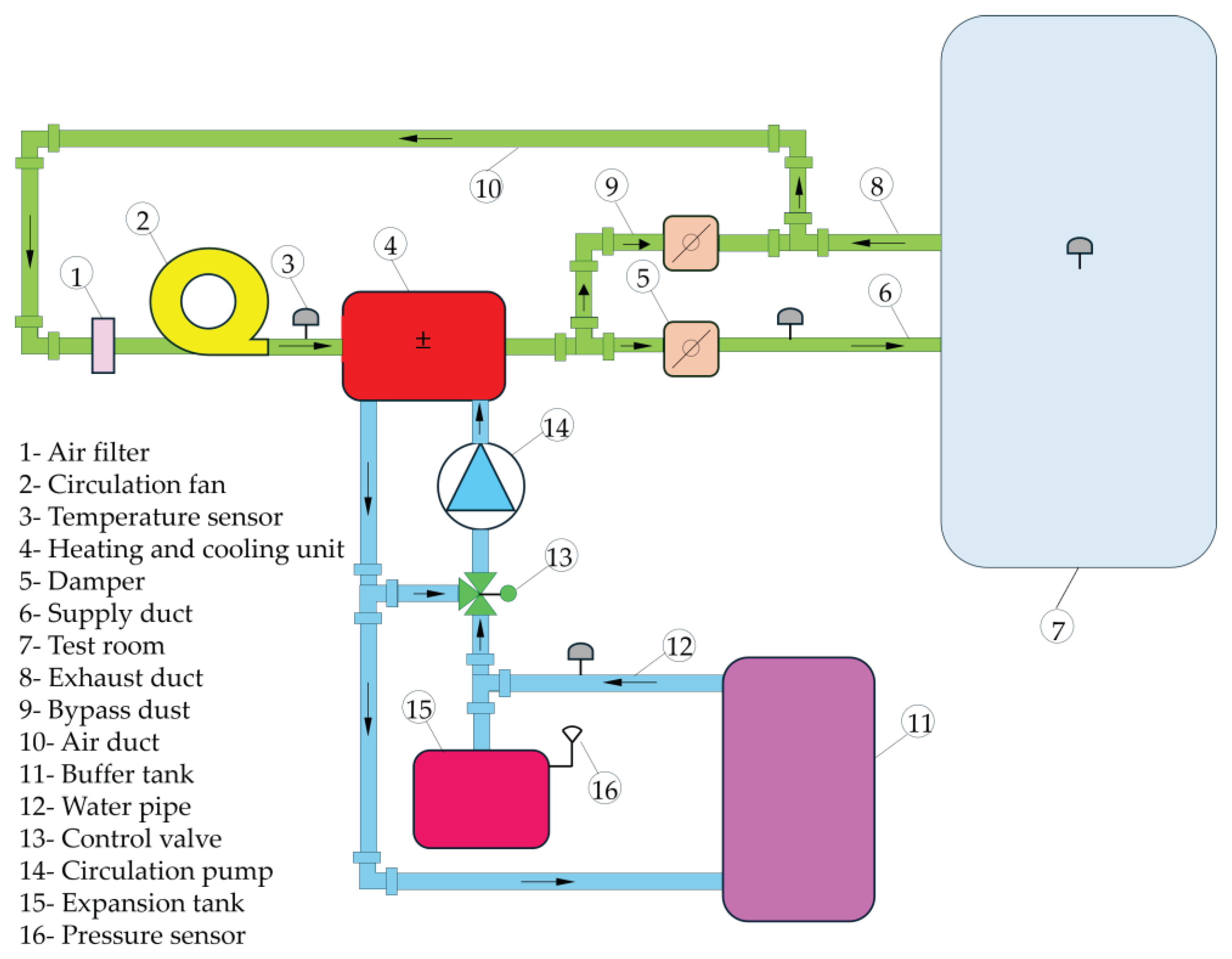
2.2. HVAC System for the Test Room

The HVAC system was a closed loop with an air handling unit (AHU) regulating the supply temperature. The conditions for heating were controlled by the feedback temperature measurement (T_spt) in the test room, which dictated whether more heating was needed whenever the temperature diverted from the set room temperature. Figure 3 shows the schematic diagram of the HVAC system used in this study.

The AHU system provided maximum airflow rates of 0.5 m³/s measured by a flow meter with an accuracy of ±5%. The flow dampers regulated the 0.5 m³/s airflow, distributing it between the bypass and supply air ducts, depending on the required airflow rate. An air filter was fitted on the ventilation duct connected to the intake air duct to remove particulate matter. A circulation fan with a maximum pressure of 0.88 kPa was placed after the air filter, and it sucked air from the test room through the air exhaust duct and air filter and discharged it into the heat exchanger for onward supply into the test room. The fan drew in the air and was the driving force for the AHU. Its high capacity made it ideal for large commercial spaces, ensuring efficient air movement through a 0.25 m diameter ventilation supply duct into the WCJ supply diffuser. The fan also sucked the air from the test room air through the air exhaust terminal and filter. The heating element in the heat exchanger had a capacity of 10 kW and heated the air to the required supply air temperature.

The supply air temperature (T_sat) depended on the designated T_spt and the outdoor air temperature (T_out). PT100 temperature sensors measured the air temperature at different positions in the AHU. A PT100, 100 Ω/0 °C, Class B temperature sensor with accuracy of ±(0.3 °C + 0.005 × |t|), where |t| is the absolute temperature [°C] and stability over a temperature range of 0 °C to +50 °C, was used for the room air temperature setpoint. The T_spt temperature sensor was integrated into the AHU, and it regulated the heating element to maintain the room air temperature setpoint despite temperature variations in the outdoor environment. The temperature sensors in the remaining parts of the AHU were PT100 EN 60751 [53] Class B with an accuracy of ± (0.3 °C + 0.005 × |t|) and a temperature range of 0 °C to 150 °C. The PT100 temperature sensors were manufactured by Produal Sverige AB, Stockholm, Sweden. The temperature measuring range enables the sensors to be used for various HVAC applications, including heating and cooling environments.

To enhance supply air heating efficiency, the AHU featured a hot water circulation circuit with a buffer tank, a circulation pump, an expansion tank, a heat exchanger, control and relief valves, pressure switches, temperature sensors, and associated piping. The heating element in the heat exchanger raised the temperature of the water in the recirculation circuit and the air in the AHU. A 0.15 m³ buffer tank temporarily stored the heated water and periodically supplied it to the heat exchanger to heat the supply air. The buffer tank optimized the heating system, improved the energy efficiency, balanced the heating load, and managed peak demand. The circulation pump, with a maximum flow rate of 0.02 m³/s, a maximum head of 18 m, a maximum pressure of 1.6 MPa, and a liquid temperature range of −10 °C to 110 °C, circulated the hot water between the heat exchanger and the buffer tank. The 0.03 m³ expansion volume tank prevented excessive pressure in the buffer tank due to the thermal expansion of water at higher temperatures.

2.3. Experimental Design

The Box–Behnken design (BBD), a response surface methodology (RSM), optimizes systems with multiple variables by efficiently organizing design variables into runs [54]. This study defines a run as a distinct combination of the number of nozzle rows (n), room air temperature setpoint (T_spt), and airflow rate ($\dot{V}$). Box–Behnken works by systematically varying the levels of the design variables in a specific pattern. Each variable is assigned three levels: low (−1), medium (0), and high (1). The center point (0) is used multiple times to estimate variability and ensure accurate quadratic modeling. These runs are randomized, and experiments are conducted according to the sequence established by the design to minimize systematic biases caused by uncontrollable factors (e.g., environmental conditions). A randomized BBD offers high efficiency with fewer runs than full factorial designs while avoiding extreme factor combinations but ensuring reliability. It provides accurate error estimates, reduces experimental bias, supports quadratic model fitting, and enhances response surface approximation, making it a robust tool for estimating first- and second-order coefficients [55,56]. The BBD is applied in many fields, including academic research [57,58].

The current experimental design included three independent variables, n, T_spt, and $\dot{V}$, each at three levels: n = 8, 10, and 12; T_spt = 18 °C, 20 °C, and 22 °C; and $\dot{V}$ = 0.3 m³/s, 0.35 m³/s, and 0.4 m³/s. This BBD resulted in 13 runs for a single center point design.

Table 1. Box–Behnken-based design of experiment showing coded and actual values of the design variables. n is the number of nozzle rows, T_spt is the room air temperature set point, and $\dot{V}$ is the flow rate.

Run	Coded Values			Actual Values
	n [-]	Tspt [°C]	$\dot{\mathit{V}}$ [m3/s]	n [-]	Tspt [°C]	$\dot{\mathit{V}}$ [m3/s]
1	1	−1	0	12	18	0.35
2	0	0	0	10	20	0.35
3	−1	−1	0	8	18	0.35
4	−1	0	−1	8	20	0.30
5	0	−1	1	10	18	0.40
6	−1	0	1	8	20	0.40
7	1	1	0	12	22	0.35
8	1	0	1	12	20	0.40
9	0	1	1	10	22	0.40
10	0	1	−1	10	22	0.30
11	1	0	−1	12	20	0.30
12	−1	1	0	8	22	0.35
13	0	−1	−1	10	18	0.30

shows randomized experimental runs obtained by the BBD method, which show coded values and actual combinations of the design variables.

Although there were no plants in the greenhouse, we selected the three T_spt values as they fell within the recommended day and night temperature range (16–24 °C) for various greenhouse crops [59,60].

2.4. Response Surface Methodology (RSM)

Response surface methodology (RSM) combines mathematical and statistical techniques to develop, improve, and optimize processes with multiple input variables. It models and predicts relationships between dependent (Y) and independent (X) variables, aiding in process optimization [54,61,62]. RSM is widely applied in fields like agriculture [63], energy systems [64], and research [57,58,65]. The methodology states that the dependent variable (Y) is related to k number of independent variables (X) according to Equation (1).

$$Y=f\left(X_1,X_2,X_3,\dots \dots ,X_k\right)+\epsilon$$

(1)

where f is an unknown response function, k is the number of independent variables, and ε is the error term due to measurement error. In this study, k = 3.

The current study used RSM to analyze the individual and combined effect of the three design variables on WCJ performance. The RSM assessed how the three design variables affect the capacity of the WCJ to heat the ceiling, external wall, and room air, as well as the WCJ supply temperature. We developed dependent (response) variables to estimate the effect of WCJ on the room air temperature (T_RAT^*), ceiling surface temperature (T_CST^*), the inner surface temperature of the external wall (T_EWT^*), and supply air temperature (T_SAT^*). The four dependent variables are dimensionless to facilitate comparisons and reveal fundamental insights across the runs. The function f represents a general response surface (RS) model, the second-order polynomial function fitted to demonstrate the correlation between the three independent variables and the respective dependent variable. The response surface (RS) model takes the form of Equation (2).

$$Y={\alpha }_0+{\sum }_{i=1}^k{\alpha }_i{X}_i+{\sum }_{i=1}^k{\alpha }_{ii}{X}_i{X}_i+{\sum }_{i=1}^k{\sum }_{j\ge 1}^k{a}_{ij}{X}_i{X}_j+\epsilon$$

(2)

where $Y$ is the dependent variable, $X_i$ and $X_j$ are the independent variables, ${\alpha }_0$ is the intercept (constant) term, ${\alpha }_i$ are the coefficients for the linear terms, ${\alpha }_{ii}$ are the coefficients for the quadratic terms, and $a_{ij}$ are the coefficients for the two-way interaction terms [54].

Equation (2) includes a constant term and three linear, three quadratic, and three two-way interaction terms with unknown coefficients. Once the dependent values are known, these coefficients are determined through least squares approximation.

RSM analysis was performed using MINITAB 2021, a statistical software widely used for data analysis, quality improvement, and process optimization. MINITAB supports diverse analyses, including statistics, predictive analytics, and experimental design, benefiting fields like quality control [66], engineering, and research [67,68,69].

2.5. Air Velocity and Temperature Measurement

Thermocouples measured the room air and surface temperatures in the research facility. Constant current anemometers (CCAs) measured the WCJ velocity and temperature in the test room. The total duration of each measurement was two days. For each run, the system was first stabilized for 12 h, followed by a 24 h measurement period with a measuring interval of 60 s. This approach ensured that the data reflected the system’s behavior under stable conditions, thereby increasing the reliability and accuracy of the results.

2.5.1. Measurements with Constant Current Anemometers (CCAs)

CCAs measured the WCJ velocity and temperature in the designated zones in the test room. CCAs were selected due to their simple design, high sensitivity, and quick response. CCAs are extensively used in meteorology, aerodynamics, HVAC optimization, and research [70,71].

Thirty-two (32) custom-fabricated CCAs with velocity and temperature sensors to measure air velocity and temperature simultaneously were installed in various zones of the test room. Each CCA probe included a 0.3 mm diameter Honeywell 111-202CAK-H02 velocity sensor. The velocity sensors were manufactured by Digi-Key Electronics from Thief River Falls, MN, USA. The Sensors were calibrated for velocities up to 20 m/s, achieving an accuracy of ±5% with a time constant of 0.5 s at 0.5 m/s and 0.1 s at 20 m/s.

Each CCA probe also featured a thermometric B43-K-5 temperature sensor calibrated up to 40 °C with ±0.05 °C accuracy. The temperature sensors were manufactured by the Thermometrics Corporation, Northridge, CA, USA. The sensors were calibrated as temperature-sensitive resistors to establish the temperature–resistance relationship with digital calibration data. The CCAs were calibrated in a controlled environment using an open-circuit wind tunnel. The CCAs were integrated into a 32-channel anemometer logger system using LabVIEW 2017. A detailed description of the operation principle of the CCAs is contained in a prior study [45].

The CCAs measured the WCJ velocity and temperature in three zones. Figure 4 shows Zone I along the ceiling, Zone II along the inner surface of the external wall, and Zone III along the floor.

In Zone I, the CCAs measured the WCJ local velocity and temperature within the boundary layer along the ceiling surface up to a band of 0.19 m. The distance from the WCJ diffuser is designated as z, and the perpendicular distance from the ceiling surface into the room is denoted by x. Five (5) CCAs were positioned at position P12 at z = 6.0 m, with x, ranging from 0.03 m to 0.19 m, and sensors spaced 0.04 m apart. The CCAs measured WCJ velocity and temperature to gain insights into WCJ attachment to the ceiling. Figure 4 shows the configuration of the CCAs at P12 in zoomed-in view A.

In Zone II, the CCAs measured WCJ local velocity and temperature within the boundary layer formed along the inner surface of the external wall. The CCAs were installed at heights designated as H = 0.7 m, H = 1.5 m, H = 2.7 m, and H = 3.5 m. Three CCAs were installed at each height with a 0.02 m spacing between adjacent sensors, and the perpendicular from the inner surface of the external wall was denoted by y, ranging from 0.02 m to 0.06 m. Figure 4 shows the orientation of the CCA sensors at each measurement height in zoomed-in view B.

In Zone III, the CCAs measured the WCJ local velocity and temperature within the boundary layer along the floor surface. Measurements were conducted at positions P1, P4, P5, P8, and P9 depicted in Figure 4. The perpendicular distance from the floor surface, denoted as H, extended to 0.13 m, with adjacent sensors spaced at 0.04 m; the closest to the floor was at 0.05. Figure 4 shows the configuration of CCA sensors at each measurement position in Zone III in zoomed-in view C.

2.5.2. Measurements with Thermocouples

Air and surface temperatures within and outside the test room were measured by T-type (copper–constantan) thermocouples, with a measuring range from −200 °C to 350 °C and an accuracy of ±0.5 °C [72]. This thermocouple type was selected due to its good stability, reasonable accuracy, and versatile operating range suitable for low to moderate temperatures. The thermocouples were connected to a 34972A LXI Data Acquisition Agilent unit and interfaced with LabVIEW Version 2017 to facilitate data acquisition. The Agilent logger was manufactured by Keysight Technologies, Inc., Santa Clara, CA, USA.

Thermocouples measured room air temperatures at positions P2, P3, P6, P7, P10, and P11 in the test room shown in Figure 4. The temperature sensor used for the room air temperature setpoint (T_spt) was positioned at a height of 2 m in the center of the test room, as shown in Figure 4. One thermocouple in the WCJ diffuser measured the supply air temperature, while another in the exhaust air terminal measured the exhaust air temperature. Additionally, one thermocouple on the greenhouse roof measured the outdoor air temperature.

Thermocouples also measured the surface temperatures for the walls, ceiling, roof, and floor. A thermocouple was placed at H = 1.5 m and H = 2.5 m on each side of the wall to measure the surface temperatures of the walls. Nineteen thermocouples measured the ceiling surface temperatures at varying distances from the WCJ diffuser, with 0.1 m spacing up to z = 1.0 m and 0.5 m spacing from z = 1.0 m to z = 6.0 m. One thermocouple was installed on the floor at 3.0 m from the external wall to measure the surface temperature. Moreover, one thermocouple was placed on the roof at z = 6.0 m to measure the roof surface temperature.

2.6. Approach and Analysis

To compare the WCJ heating performance, the temperatures on the ceiling, external wall, supply air, and room air across runs are non-dimensioned. The effect of the outdoor air temperature on the room air temperature, ceiling surface temperature, inner surface temperature of the external wall, and WCJ supply air temperature is incorporated in the analysis by using the dimensionless variables. These dimensionless parameters became the dependent (response) variables in the RSM analysis.

2.6.1. The Dimensionless Ceiling Surface Temperature (T_CST^*)

To investigate how the three design variables influence the heating effect of the WCJ on the ceiling surface, the ceiling surface temperature is non-dimensioned using Equation (3).

$${T_{\mathrm{C}\mathrm{S}\mathrm{T}}}^{*}={\displaystyle \frac{\left(T_{\mathrm{c}\mathrm{s}\mathrm{t}}-T_{\mathrm{o}\mathrm{u}\mathrm{t}}\right)}{\left(T_{\mathrm{s}\mathrm{p}\mathrm{t}}-T_{\mathrm{o}\mathrm{u}\mathrm{t}}\right)}}$$

(3)

where (T_cst) is the ceiling surface temperature [°C], (T_out) is the outdoor air temperature [°C], (T_spt) is the room air temperature setpoint [°C], and (T_out) is the outdoor air temperature [°C].

The dimensionless ceiling surface temperature indicates the relative magnitude of the ceiling’s temperature compared to the desired indoor conditions. A higher value suggests a better insulating effect the WCJ provides on the ceiling surface.

2.6.2. The Dimensionless Inner Surface Temperature of the External Wall (T_EWT^*)

Similarly, to assess the heating effect of the WCJ on the inner surface of the external wall, the dimensionless inner surface temperature was defined as:

$${T_{\mathrm{E}\mathrm{W}\mathrm{T}}}^{*}={\displaystyle \frac{\left(T_{\mathrm{e}\mathrm{w}\mathrm{t}}-T_{\mathrm{o}\mathrm{u}\mathrm{t}}\right)}{\left(T_{\mathrm{s}\mathrm{p}\mathrm{t}}-T_{\mathrm{o}\mathrm{u}\mathrm{t}}\right)}}$$

(4)

where (T_ewt) is the inner surface temperature of the external wall [°C].

T_EWT^* reflects how effectively the WCJ insulates the inner wall surface from the colder outdoor environment.

2.6.3. The Dimensionless Supply Air Temperature (T_SAT^*)

To maintain the specified operational room air temperature setpoint, the AHU control system adjusts the supply air temperature to compensate for heat losses through the building envelope due to variations in outdoor conditions. The T_SAT^* value represents the relative supply air temperature (T_sat) increase required to achieve the operational indoor setpoint temperature, accounting for outdoor temperature variations. The dimensionless supply air temperature is calculated as:

$${T_{\mathrm{S}\mathrm{A}\mathrm{T}}}^{*}={\displaystyle \frac{\left(T_{\mathrm{s}\mathrm{a}\mathrm{t}}-T_{\mathrm{o}\mathrm{u}\mathrm{t}}\right)}{\left(T_{\mathrm{s}\mathrm{p}\mathrm{t}}-T_{\mathrm{o}\mathrm{u}\mathrm{t}}\right)}}$$

(5)

2.6.4. The Dimensionless Room Air Temperature (T_RAT^*)

The main objective of using a warm WCJ is to create an air boundary layer with an insulating effect along the envelope surfaces (ceiling and external wall) to create and maintain the required indoor air temperature (T_rat) at the desired setpoint. To evaluate the WCJ’s effectiveness in achieving this goal, we defined the dimensionless room air temperature (T_RAT^*) as:

$${T_{\mathrm{R}\mathrm{A}\mathrm{T}}}^{*}={\displaystyle \frac{\left(T_{\mathrm{r}\mathrm{a}\mathrm{t}}-T_{\mathrm{o}\mathrm{u}\mathrm{t}}\right)}{\left(T_{\mathrm{s}\mathrm{p}\mathrm{t}}-T_{\mathrm{o}\mathrm{u}\mathrm{t}}\right)}}$$

(6)

3. Results and Discussion

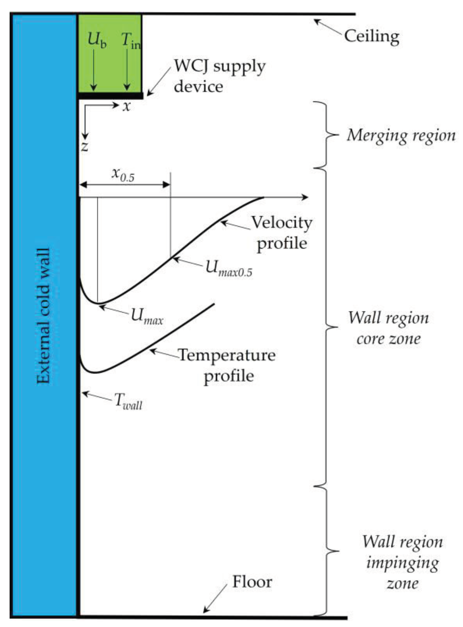
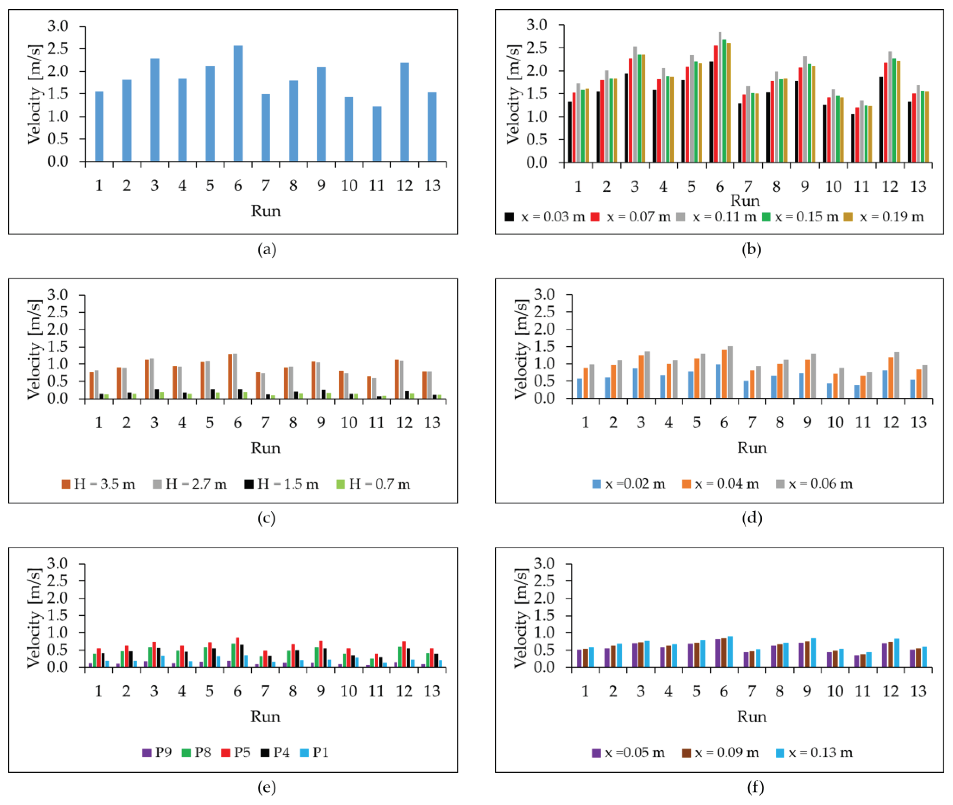
This section presents the results of an experimental investigation on the potential of the warm WCJ to climatize a greenhouse exposed to transient weather conditions. This section is divided into multiple subsections, presenting results, discussing their implications, and revealing the warm WCJ’s capacity to create optimum indoor airflow and a thermal environment relative to the setpoint. However, any analysis related to heat transfer quantities between the WCJ and the external wall and the ceiling to combat the heat loss through these external surfaces is postponed and will be reported in a future article focusing on the energy performance of the WCJ heating system.

3.1. WCJ Velocity

In the current study, the warm WCJ flowed attached to the ceiling, onto the external wall, and, finally, along the floor before being exhausted from the test room. The path of the WCJ was traced by measuring the local air velocity and temperature in the boundary layer that it created along the ceiling surface (Zone I), the inner surface of the external wall (Zone II), and the floor (Zone III). Figure 5a shows the average WCJ velocity at P12 in Zone I. Figure 5b shows the distribution of the WCJ velocity in the band of x = 0.19 m at P12 in Zone I. Figure 5c shows the average WCJ velocity at different heights along the inner surface of the external wall in Zone II. Figure 5d shows a representative WCJ velocity distribution in the band y = 0.6 m at H = 2.7 m to demonstrate the WCJ velocity distribution at various heights along the inner surface of the external wall in Zone II. Figure 5e shows the average WCJ velocity at different points along the floor in Zone III of the test room. Figure 5f displays the WCJ velocity distribution in the band H = 0.13 m at P5 to represent the velocity distribution along the floor in Zone III.

Figure 5a shows that the WCJ velocity differed based on the airflow rate and number of nozzle rows. Run 6 shows the highest velocity with the highest airflow rate and lowest n, while Run 11 shows the opposite.

Figure 5b shows the WCJ velocity magnitude that indicates that the jet flow remains attached to the ceiling, forming a boundary layer and reaching the end of the ceiling with sufficient momentum across all runs. This is evident in run 11, which has the highest number of nozzles and the lowest airflow rate yet still maintains a velocity greater than 1.2 m/s at x = 0.03 m. The flow behavior along the ceiling indicates the WCJ characteristic flow behavior and thus confirms the results obtained in prior laboratory studies [45,73].

Figure 5c shows that the average WCJ velocity decreases as it propagates towards the floor, being highest at H = 3.5 m and lowest at H = 0.7 m. As expected, the magnitude of the WCJ velocity decreased with an increase in distance from the WCJ supply diffuser, with the highest values at H = 3.5 m and the lowest at H = 0.7 m. The velocity at H = 1.5 m is unusually low because of the obstruction imposed by a support channel to the greenhouse’s external wall. Moreover, the WCJ velocity reduces as the jet approaches the floor due to the obstruction and compressive effect of the floor, as illustrated at H = 0.7. Run 6 shows the velocity of 1.5 m/s at H = 3.5 m and 0.2 m/s at H = 0.7 m.

Figure 5d shows the WCJ flow behavior in the boundary layer in Zone II at H = 2.7 m, where the velocity is measured away from disturbances after the jet regains momentum lost at the ceiling external wall corner. The WCJ velocity increases with distance from the external wall, i.e., the WCJ velocity is highest at x = 0.06 m.

Figure 5e shows that the WCJ retains sufficient momentum to continue propagating along the floor, as indicated by high velocities at all points except P9, which is closest to the external wall. A lower velocity was measured at P9 because of its location in a recirculation bubble, which is expected to be created at the external wall–floor corner. However, the WCJ regains its momentum and accelerates into the room. The highest velocity was recorded at P5, a point that benefits from its central location and minimal interference from surrounding walls. The WCJ velocity at P5 represents the airflow in the room. For the studied runs, the near-floor air velocities ranged between 0.2 m/s and 0.7 m/s, representing an optimal range for diverse crops at various growth stages.

Figure 5f shows a similar trend as that observed in Zone III, in which the velocity increases with the distance from the surface. Velocities of about 0.3 m/s to 0.5 m/s are measured in Zone III. The results illustrate that the air distribution system operated according to the stated design variables can deliver a WCJ with a velocity that meets the recommended air movements for several greenhouse crops. Previous studies recommend that velocities below 0.5 m/s suit germinating seeds, seedlings, and delicate crops sensitive to excessive airflow. Velocities ranging from 0.5 m/s to 1.0 m/s are suitable for most greenhouse crops, including tomatoes, peppers, lettuce, and herbs, during their vegetative growth phase [60,74]. This knowledge aids ventilation and air distribution system manufacturers in designing suitable air supply diffusers for greenhouses and other large-space buildings. It also helps greenhouse crop farmers and operators select the correct airflow rates for crop-specific air movement needs. However, further studies in greenhouses with live plants are necessary to assess how plants affect airflow patterns and temperature distribution in the test room.

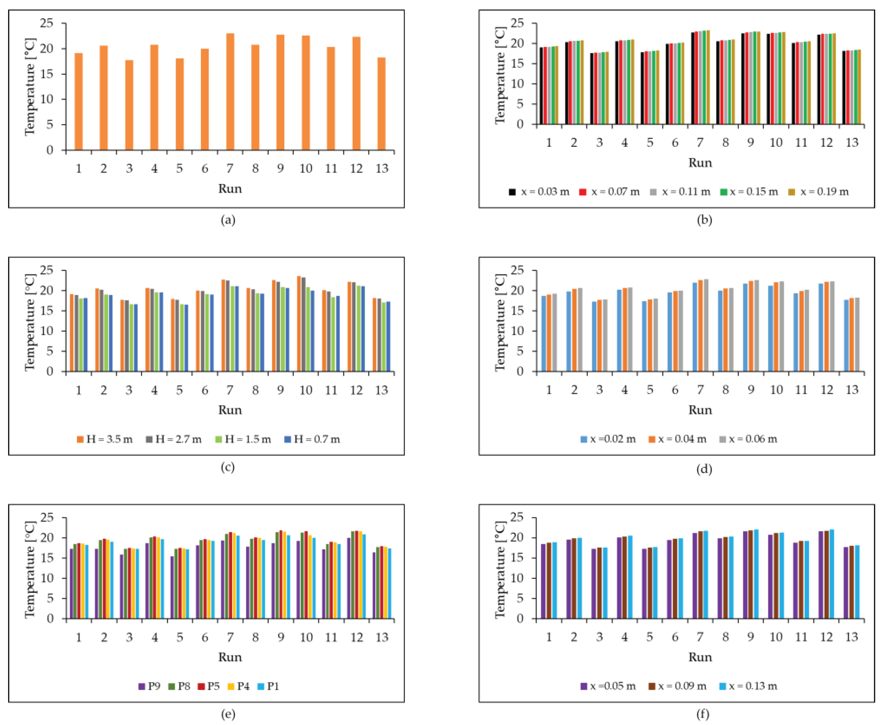
3.2. WCJ Temperature

Figure 6 shows the CCA-measured WCJ temperature in the three zones. Figure 6a shows the average WCJ temperature at P12 in Zone I. Figure 6b shows the distribution of the WCJ temperature along the ceiling at P12 in Zone I. Figure 6c shows the average WCJ temperature at different heights along the inner surface of the external wall in Zone II. Figure 6d shows representative WCJ temperature distribution at H = 2.7 m to demonstrate the WCJ temperature at various heights along the inner surface of the external wall in Zone II. Figure 6e shows the average WCJ temperature at different points along the floor in Zone III of the test room. Figure 6f displays the WCJ temperature distribution profile at P5 to present the temperature along the floor in Zone III.

Figure 6a indicates that T_spt strongly influenced the WCJ temperature along the ceiling, as shown by the higher values in runs 7, 9,10, and 12, which have T_spt = 22 °C, compared to runs 3, 5, and 13 with T_spt = 18 °C.

Figure 6b shows the WCJ temperature distribution with the temperature increasing slightly away from the ceiling, with the highest at x = 0.19. This follows the trend observed in the WCJ velocity distribution because velocity is the heat transport mechanism. However, the temperature difference between adjacent measurement points is marginal. The WCJ temperature is lower closer to the ceiling surface because of the influence of the cold outdoor environment. A combination of higher room air temperature setpoints and lower airflow rates causes a higher WCJ temperature along the ceiling, as shown by run 10. Conversely, run 5 shows that a lower T_spt and a higher $\dot{V}$ cause a lower WCJ temperature along the ceiling. At P12, the WCJ temperature exceeds T_spt, as evidenced in runs 1 and 7. The band of warm WCJ shields the room air by isolating the indoor and external environments. This shielding layer of the WCJ provides an insulating effect on the ceiling surface by limiting the influence of the lower winter outdoor air temperatures by transferring heat to the ceiling. The flow behavior illustrates that the WCJ transfers heat to the ceiling and the ambient room air, raising their temperatures. The heating of the ceiling would prevent condensation of the moisture-laden indoor air on the surface due to the lower outdoor air temperature. Condensation due to evapotranspiration and irrigation causes fungal diseases in greenhouses [60,75].

Figure 6c shows that the WCJ loses heat as it flows along the ceiling; it further loses heat along the external wall as indicated by the higher temperature at H = 3.5 m and lowest at H = 0.7 m, with a temperature difference of between 0.9 °C and 2 °C depending on T_spt and the outdoor air temperature.

Figure 6d shows a similar trend where the lowest temperature lies closest to the inner surface of the external wall; however, the difference between adjacent points is negligible.

Figure 6e shows that the WCJ temperature in Zone III closely approximates the setpoint for the room air temperature. The WCJ temperature remained uniform throughout the room, except at P9, which was slightly lower due to being situated in the recirculation bubble. This illustrates that the jet transfers heat to the relatively cooler room air, thus raising its temperature.

Figure 6f indicates that the WCJ temperature increases slightly with an increase in H. The near-floor air temperature at P5 consistently matched T_spt, illustrating that the WCJ transferred heat to elevate the room air temperature.

3.3. Effect of Warm WCJ on the Ceiling Surface

To estimate the heating effect of the WCJ, the dimensionless ceiling surface temperature (T_CST^*) in Equation (3) was used. The WCJ insulation capacity was estimated by equating it to the ceiling surface temperature due to the heat transfer between the warm WCJ and the cold ceiling. The insulation capacity is a function of the room air temperature setpoint and outdoor air temperature and is represented by T_CST^*. Thus, a higher ceiling surface temperature denotes higher insulating capacity, and vice versa.

3.3.1. Dynamic Dimensionless Ceiling Surface Temperature (T_CST^*) Profiles

The measured ceiling surface temperature at different distances from the WCJ diffuser is non-dimensioned and presented in Figure 7. Figure 7a–c show the effect of the design variables on the insulating effect of the WCJ on the ceiling surface under a variable outdoor air temperature (T_out). In Figure 7a, the impact of $\dot{V}$ and n on T_CST^* is shown while maintaining T_spt at 20 °C. Figure 7b explores the effect of T_spt and the number of nozzle rows (n) on T_CST^* with $\dot{V}$ held constant at 0.35 m³/s. Figure 7c demonstrates the influence of $\dot{V}$ and T_spt on T_CST^* while keeping n at 10.

Figure 7a shows that T_CST^* reduces as the airflow rate increases and n decreases. T_CST^* reduces due to decreased convective heat transfer within the boundary layer because the WCJ spends less time in contact with the ceiling surface, as seen by the difference in runs 4 and 6. This shorter residence time limits heat exchange between the WCJ and the colder ceiling. Moreover, a higher $\dot{V}$ results in less heating of the supply air by the air distribution system to meet T_spt, further contributing to reduced T_CST^*. In contrast, the WCJ heating effect is higher at a higher airflow rate and number of nozzle rows, as shown in the differences between runs 6 and 8. This is attributed to the increased shielding effect for higher n, the jet’s contact time, and the contact surface area for a lower $\dot{V}$, enhancing convective heat transfer through thicker boundary layers and the ceiling.

Figure 7b illustrates that an increase in n correlates with an increase in T_CST^*, attributed to the formation of a boundary layer by the warm WCJ, thereby enhancing heat transfer from the jet to the ceiling surface. Additionally, the velocity and momentum of the WCJ are conserved, resulting in a higher mass flow rate reaching the ceiling and augmenting heat transfer. A higher $\dot{V}$ and fewer n contribute to thin boundary layers that promote direct contact between the warm WCJ and the cold ceiling surface, further enhancing the heating effect. Furthermore, T_CST^* is enhanced by increased T_spt because the corresponding WCJ is supplied at higher temperatures, as demonstrated by runs 3 and 12.

Figure 7c demonstrates a positive correlation between T_CST^* and T_spt, as shown by runs 5 and 9. T_CST^* tends to increase with a reduction in $\dot{V}$, as illustrated by runs 10 and 13. Under the stated conditions, the increase in T_CST^* is attributed to the higher supply temperatures.

The heating effect is lower closer to the WCJ diffuser at z = 0.0 m and z = 0.1 m because the WCJ is not yet attached to the ceiling surface. T_CST^* is highest at about z = 0.5 m, indicating that the warm WCJ attaches to the ceiling surface and transfers heat to the surface. The heating effect reduces as the distance from the WCJ diffuser increases. A T_CST^* value between 0.95 and 1.1 is adequate to insulate the ceiling surface to maintain the required indoor air temperature.

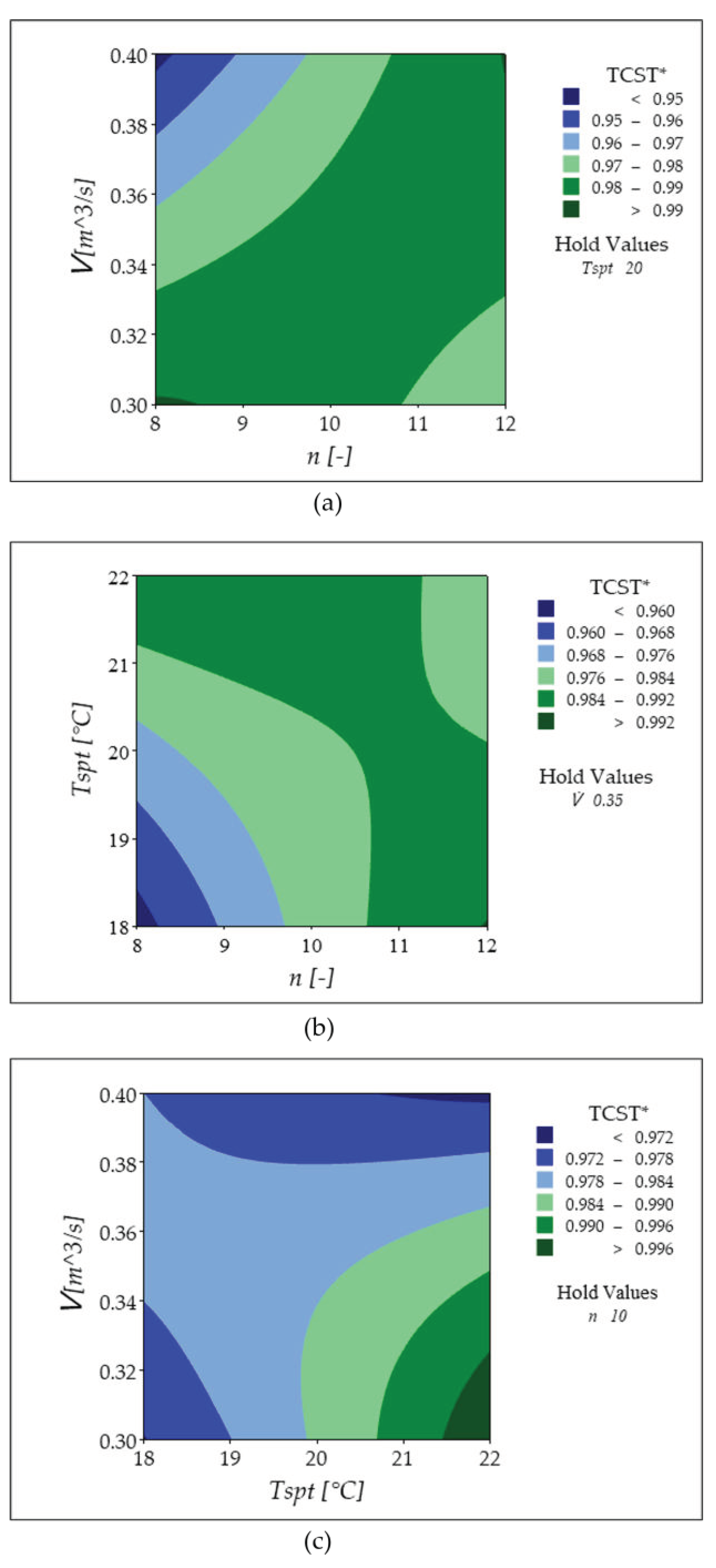
3.3.2. Contour Plots of Dimensionless Ceiling Surface Temperatures

Contour plots show the effects of the interaction between two independent design variables on the dependent variables, keeping the third design variable constant at its mid-level value. Color-coded regions highlight different value ranges, with darker blue indicating lower values and darker green indicating higher values. In Figure 8a, the impact of $\dot{V}$ and n on T_CST^* is shown while maintaining T_spt at 20 °C. Figure 8b explores the effect of T_spt and n on T_CST^* with $\dot{V}$ held constant at 0.35 m³/s. Figure 8c demonstrates the influence of $\dot{V}$ and T_spt on T_CST^* while keeping n at 10.

Figure 8a shows that T_CST^* increases as $\dot{V}$ decreases, and the effect is more pronounced at a lower n. While both a higher n and a higher $\dot{V}$ contribute to a rise in T_CST^*, a lower $\dot{V}$ combined with a higher n leads to a decrease in T_CST^*. The heating effect intensifies as n increases up to a certain threshold, beyond which it starts to decline unless accompanied by a rise in $\dot{V}$. This suggests that the WCJ supply diffuser design should have an optimal range for n to maximize heating efficiency.

Figure 8b shows that T_CST^* increases with an increase in T_spt and n. The influence of n on T_CST^* is more significant at a higher T_spt. This thermal behavior is due to higher supply air temperatures, which cause the warm WCJ to supply more heat to the ceiling.

Figure 8c shows that T_CST^* increases with T_spt but decreases with an increase in $\dot{V}$. This indicates an inverse relationship between $\dot{V}$ and T_CST^*. The potential of the WCJ’s heating effect on the ceiling surface increases as T_spt increases but decreases as $\dot{V}$ increases. Increasing $\dot{V}$ outweighs positively impacting T_CST^* when interacting with n but can have a negative effect when interacting with T_spt.

3.3.3. Response Surface Model for Dimensionless Ceiling Surface Temperature (T_CST^*)

Equation (7) is the regression equation of the response surface (RS) model, which estimates the effects of linear terms, quadratic terms, and two-way interaction terms on T_CST^*.

$$\begin{gathered} {T_{\mathrm{C}\mathrm{S}\mathrm{T}}}^{*}=0.09+0.029n+0.051T_{\mathrm{s}\mathrm{p}\mathrm{t}}+1.22\dot{V}-0.00107n\times n+0.00034T_{\mathrm{s}\mathrm{p}\mathrm{t}}\times T_{\mathrm{s}\mathrm{p}\mathrm{t}}-1.58\dot{V}\times \dot{V} \\ -0.00301 n\times T_{\mathrm{s}\mathrm{p}\mathrm{t}}+0.159n\times \dot{V}-0.091T_{\mathrm{s}\mathrm{p}\mathrm{t}}\times \dot{V} \end{gathered}$$

(7)

The R² for RS Equation (7) is 57%, indicating a moderate correlation. Equation (7) suggests that increasing $\dot{V}$ initially raises T_CST^* but reduces it beyond a certain point due to the negative quadratic term. For n, more jets increase T_CST^*, though with diminishing returns as n rises. The positive interaction between n and $\dot{V}$ boosts T_CST^*. Increasing T_spt also raises T_CST^*, though its quadratic effect is minor. However, the negative interaction between T_spt and $\dot{V}$ suggests that raising both will lower T_CST^*.

3.4. Effect of the Warm WCJ on the External Wall

To estimate the heating capacity of the WCJ, the dimensionless inner surface temperature of the external wall (T_EWT^*) in Equation (4) was used. The higher the T_EWT^* value, the higher the insulation the WCJ offers.

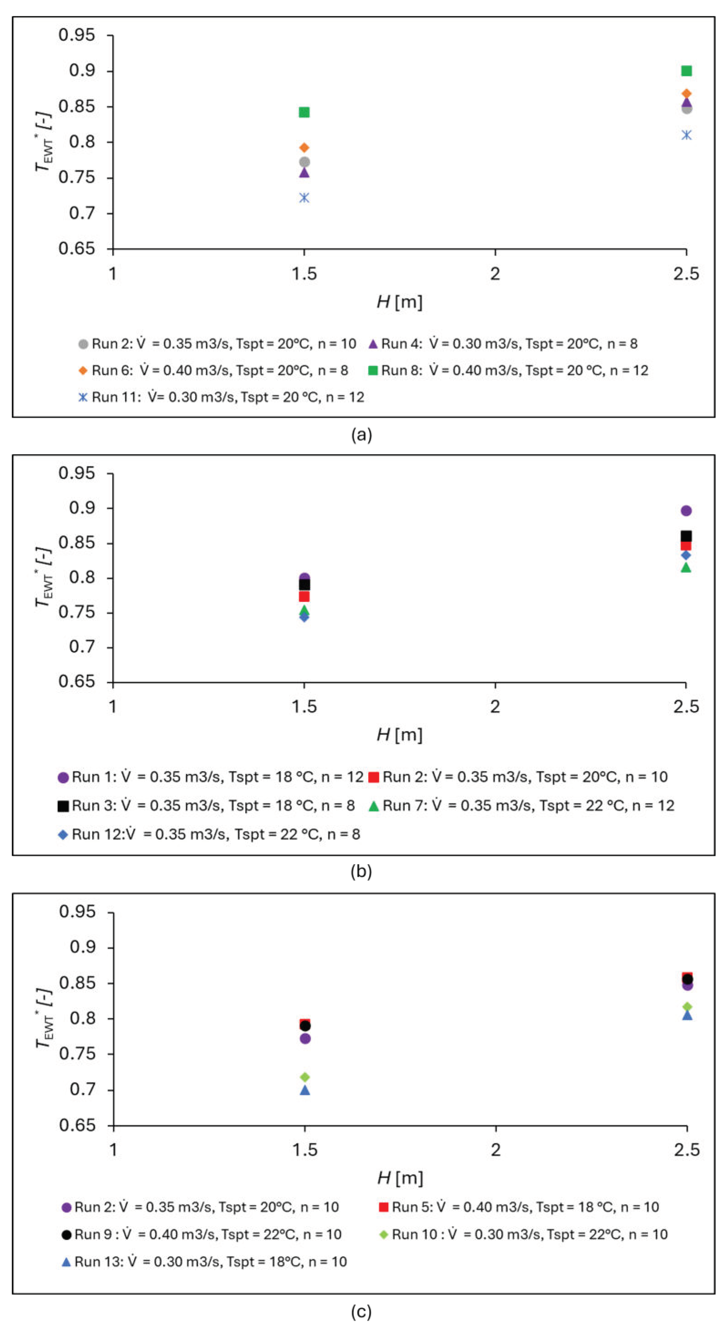
3.4.1. The Dynamic Dimensionless Inner Surface Temperature of the External Wall (T_EWT^*)

Figure 9a–c illustrate the variation in T_EWT^* over 24 h, depending on the interaction of three independent variables and the outdoor air temperature. Figure 9a depicts the impact of $\dot{V}$ and n on T_EWT^* while maintaining T_spt at 20 °C. Figure 9b shows the effect of T_spt and n on T_EWT^* with $\dot{V}$ fixed at 0.35 m³/s. Figure 9c illustrates the influence of $\dot{V}$ and T_spt on T_EWT^* with n held constant at 10.

Figure 9a illustrates that at a constant T_spt, T_EWT^* rises with increasing $\dot{V}$ and n, as shown by runs 6 and 8. T_EWT^* increases with an increase in $\dot{V}$ because of the higher mass flow rate that raises the heat transfer rates from the jet to the cold external surface. WCJs supplied at a lower $\dot{V}$ and a higher n have a reduced mass flow rate and momentum by the time they flow along the inner surface of the external wall due to the elongated propagation distance from the WCJ diffuser, as shown by run 11.

Figure 9b indicates that at a designated $\dot{V}$, T_EWT^* increases as n decreases due to the higher jet velocity and momentum, which creates a thin boundary layer, enhancing heat transfer to the cold external wall, as shown in run 3. Run 1 indicates that T_EWT^* increases with a higher n at a lower T_spt due to enhanced shielding effect. T_EWT^* rises as T_spt decreases because of the higher mass flow rate which enhances heat transfer, as demonstrated by run 12.

Figure 9c shows that T_EWT^* increases with the rise in $\dot{V}$ and T_spt. Higher $\dot{V}$ values enhance the heating capacity due to a higher supply velocity and mass flow rate, as illustrated by runs 5 and 9. Increased T_spt values lead to a more significant temperature difference between the WCJ and the cold surface, facilitating heat transfer to the surface. Elevated supply air temperatures enhance convective heat transfer, accelerating surface temperature rise. The airflow patterns created by the WCJ air distribution strategy maintain adequate jet momentum across all airflow rates to effectively heat the cold external wall, albeit to varying extents.

The WCJ insulating effect on the external wall is lower than that of the ceiling because the jet loses its heat as the distance from the diffuser increases due to heat transmission through the ceiling and mixing with ambient room air. A T_EWT^* value between 0.75 and 0.95 is adequate to heat the external wall to maintain the required indoor thermal environment.

3.4.2. Contour Plots for the Dimensionless Inner Surface Temperature of the External Wall (T_EWT^*)

Figure 10a–c demonstrate how n, $\dot{V}$, and T_spt affect the heating effect of the WCJ on the inner surface of the external wall.

Figure 10a shows that T_EWT^* increases as both $\dot{V}$ and n increase. T_EWT^* increases with n up to a certain point, after which it slightly decreases, only to increase again as the increase in n continues.

Figure 10b indicates that T_EWT^* is higher at a lower T_spt. T_EWT^* increases with n with a portion of decline between n = 9 and n = 11. The impact of n on T_EWT^* is more significant at lower T_spt values.

Figure 10c indicates that T_EWT^* is higher at a lower T_spt and a higher $\dot{V}$. This is attributed to the high thermal energy content due to the high WCJ velocity and mass flow rate reaching the external wall after a long distance. The interaction between T_spt and $\dot{V}$ indicates that increasing both variables has a counteractive effect on T_EWT^*. A lower $\dot{V}$ and higher T_spt lead to lower T_EWT^*, which is attributed to a low mass flow rate.

3.4.3. Response Surface for the Dimensionless Inner Surface Temperature of the External Wall (T_EWT^*)

Equation (8) provides the regression equation of the response surface (RS) model, estimating the effects of linear terms, quadratic terms, and two-way interaction terms on T_EWT^*.

$$\begin{gathered} {T_{\mathrm{E}\mathrm{W}\mathrm{T}}}^{*}=-0.28-0.071n+0.073T_{\mathrm{s}\mathrm{p}\mathrm{t}}+3.84\dot{V}+0.00258n\times n-0.00139T_{\mathrm{s}\mathrm{p}\mathrm{t}}\times T_{\mathrm{s}\mathrm{p}\mathrm{t}}-4.98\dot{V}\times \dot{V} \\ -0.00079 n\times T_{\mathrm{s}\mathrm{p}\mathrm{t}}+0.098n\times \dot{V}-0.040T_{\mathrm{s}\mathrm{p}\mathrm{t}}\times \dot{V} \end{gathered}$$

(8)

Equation (8) has an R² value of 78%, indicating a strong correlation. It shows that increasing $\dot{V}$ initially raises T_EWT^*, but further a increase, reduces it due to the negative quadratic term. Increasing n decreases T_EWT^* at first, but after a threshold, it raises it. The interaction between n and $\dot{V}$ positively boosts T_EWT^*. While a higher T_spt increases T_EWT^*, its effect diminishes at higher values. The negative interaction between T_spt and $\dot{V}$ suggests that increasing both lowers T_EWT^*.

3.5. WCJ Supply Temperature

The AHU adjusted the WCJ supply temperature to compensate for the ceiling and external wall heat loss due to the cold outdoor air temperature (T_out) to create the required room air temperature dictated by design T_spt. Equation (5) provided a non-dimensional supply air temperature (T_SAT^*) formulation to compare across the runs.

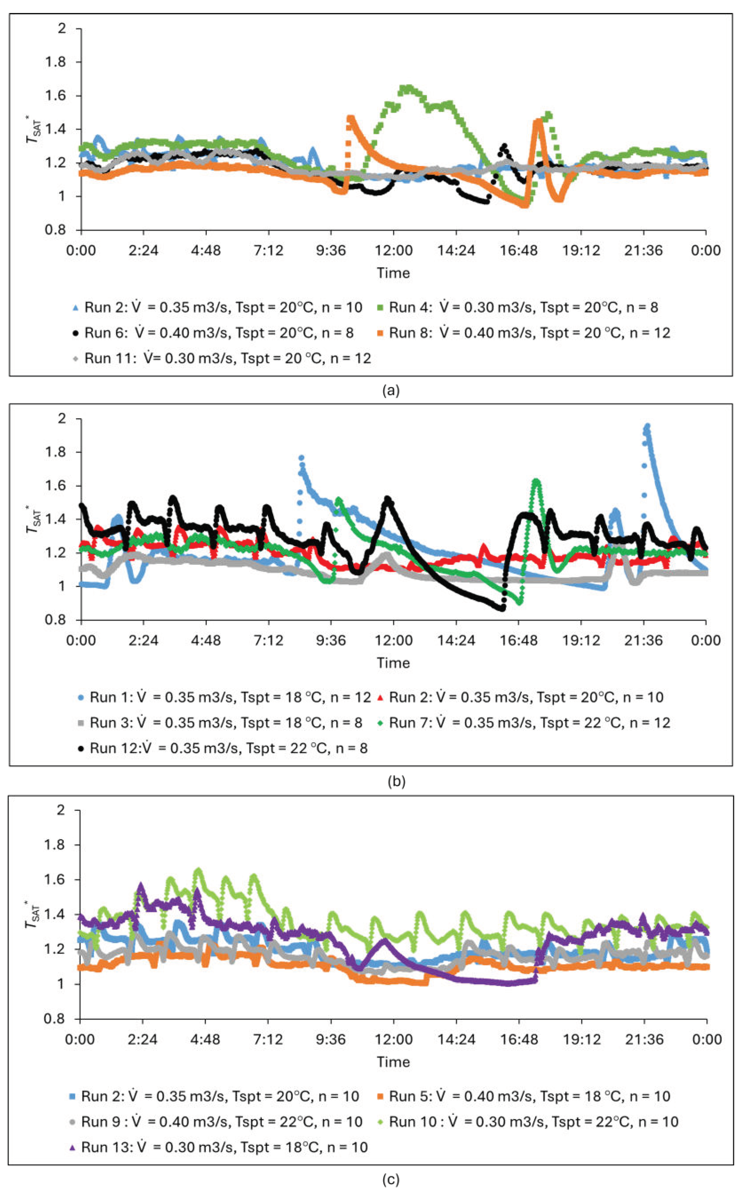
3.5.1. Dynamic Dimensionless Supply Air Temperature (T_SAT^*)

Figure 11a–c show the T_SAT^* profiles over 24 h. Figure 11a shows the impact of $\dot{V}$ and n on T_SAT^* while keeping T_spt at 20 °C. Figure 11b shows the effect of T_spt and n on T_SAT^* with $\dot{V}$ fixed at 0.35 m³/s. Figure 11c shows the influence of $\dot{V}$ and T_spt on T_SAT^* while keeping n at 10.

Figure 11a illustrates that as $\dot{V}$ decreases, T_SAT^* increases, as demonstrated by runs 4 and 11. Runs 6 and 8 demonstrate opposing trends: in run 6, increasing $\dot{V}$ while reducing the n raises the supply temperature, whereas in run 8, increasing both $\dot{V}$ and n lowers it.

Figure 11b shows that increasing T_spt and lowering n leads to a rise in T_SAT^*, as seen in runs 7 and 12, although T_SAT^* increases as n increases at a lower T_spt, as indicated by runs 1 and 3.

Figure 11c demonstrates that reducing $\dot{V}$ and increasing T_spt both raise T_SAT^*, as illustrated in runs 10 and 13. An increase in T_SAT^* parallels a decrease in $\dot{V}$, whereas a rise in T_spt correlates positively with an increase in T_SAT^*. An elevated supply air temperature enhances convective heat transfer, thereby increasing thermal energy exchange between the WCJ and ceiling surface, WCJ and external wall surface, and the warm WCJ and room air. The results indicate that a T_SAT^* value of about 1.2 is adequate to compensate for the heat loss across the building envelope exposed to varying winter temperatures. The bulging in profiles seen in runs 1, 4, 7, 8, and 12 in Figure 11a,b during the afternoon can be attributed to sunlight exposure. The air distribution system was configured primarily for heating and did not provide immediate cooling when temperatures exceeded the setpoint.

A negative correlation exists between outdoor and supply air temperatures: as outdoor temperatures drop, higher supply air temperatures are needed to maintain T_spt. A large temperature difference between the indoor surfaces of the ceiling and external wall and the cold outdoor air increases heat loss, which the system offsets by raising the supply air temperature. This study showed that the maximum supply air temperatures ranged from 27 °C to 40 °C, showing that low-temperature heating systems can effectively heat greenhouses with WCJ supply diffusers. The field studies took place in a greenhouse near a steel industry producing excess waste heat, aiming to utilize low-exergy energy (under 50 °C), which is generally unsuitable for industrial use but ideal for mild heating needs, like space heating in greenhouses.

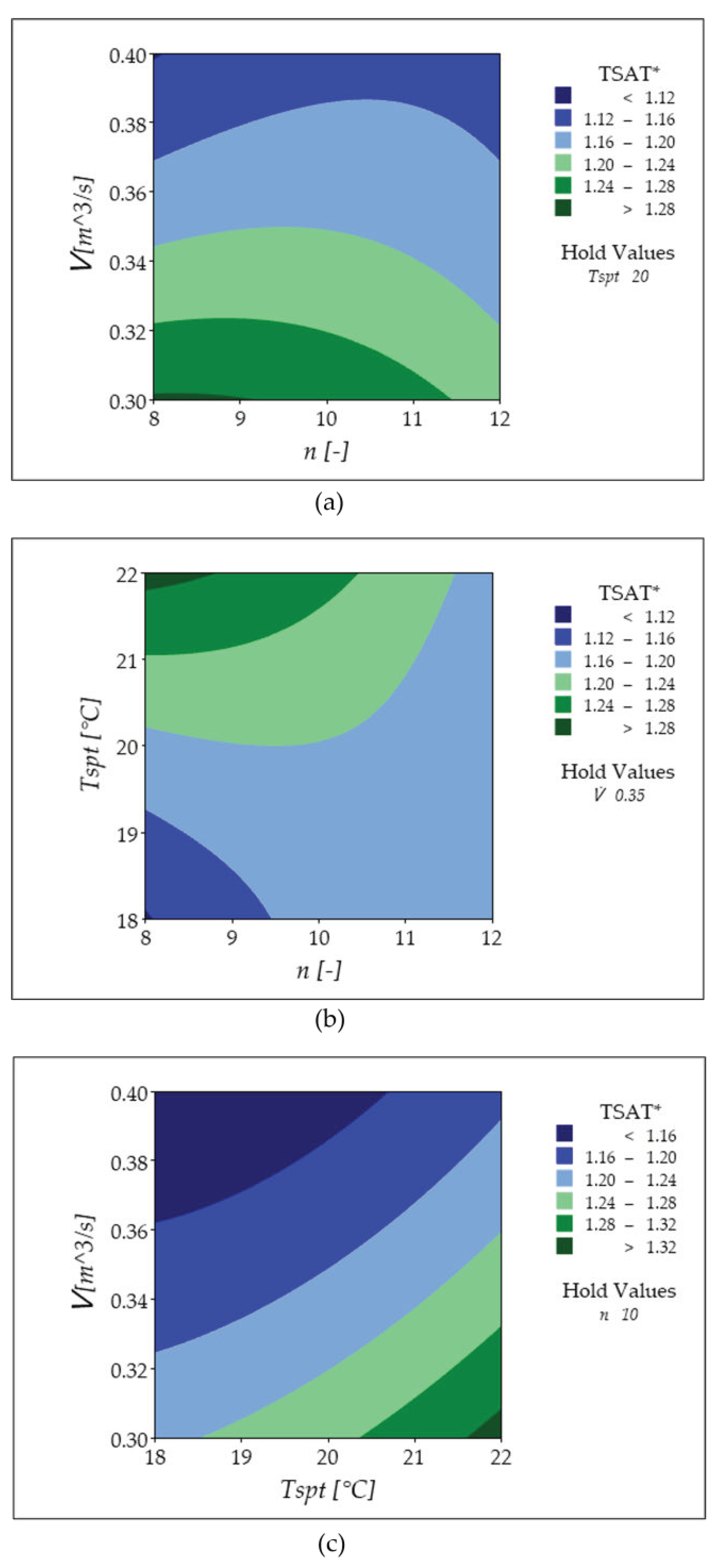
3.5.2. Contour Plots for Supply Air Temperature (T_SAT^*)

Figure 12a–c demonstrate how n, $\dot{V}$, and T_spt affect the WCJ supply temperature, represented by the dimensionless supply air temperature (T_SAT^*). Figure 12a shows the impact of $\dot{V}$ and n on T_SAT^* while keeping T_spt at 20 °C. Figure 12b shows the effect of T_spt and n on T_SAT^* with $\dot{V}$ fixed at 0.35 m³/s. Figure 12c shows the influence of $\dot{V}$ and T_spt on T_SAT^* while keeping n at 10.

Figure 12a shows that T_SAT^* increases as $\dot{V}$ and n decreases. To reach T_spt, the air distribution system raised the supply temperature at a lower $\dot{V}$ and n to offset the reduced heat-carrying capacity of the velocity because of the low mass flow rate. An inverse relationship exists between T_SAT^* and the interaction of $\dot{V}$ and n. Figure 12b illustrates that T_SAT^* increases with a rise in T_spt at a lower n. This is caused by the high supply air temperature at which the WCJ would have to be supplied to create and maintain the indoor room air temperature at the corresponding high T_spt. Figure 12c demonstrates that T_SAT^* increases as $\dot{V}$ decreases and T_spt increases.

3.5.3. Response Surface for Dimensionless Supply Air Temperature (T_SAT^*)

Equation (9) provides the regression equation of the response surface (RS) model, which estimates the effects of linear terms, quadratic terms, and two-way interaction terms of the three design variables on T_SAT^*.

$$\begin{gathered} {T_{\mathrm{S}\mathrm{A}\mathrm{T}}}^{*}=0.42+0.236n+0.036T_{\mathrm{s}\mathrm{p}\mathrm{t}}-4.2\dot{V}-0.00423n\times n+0.00344T_{\mathrm{s}\mathrm{p}\mathrm{t}}\times T_{\mathrm{s}\mathrm{p}\mathrm{t}}+4.1\dot{V}\times \dot{V} \\ -0.01163 n\times T_{\mathrm{s}\mathrm{p}\mathrm{t}}+0.218n\times \dot{V}-0.105T_{\mathrm{s}\mathrm{p}\mathrm{t}}\times \dot{V} \end{gathered}$$

(9)

Equation (9) has an R² value of 88%, indicating a very strong correlation. The negative linear term for $\dot{V}$ shows that increasing $\dot{V}$ decreases T_SAT^*, but the positive quadratic term suggests that beyond a point, further increases raise T_SAT^*. A higher n increases T_SAT^*, though with diminishing returns. The interaction between n and $\dot{V}$ also boosts T_SAT^*. Increasing T_spt raises T_SAT^*, with a minor increase at higher levels. However, the interaction between T_spt and $\dot{V}$ is negative; increasing both lowers T_SAT^*.

3.6. Room Air Temperature

The warm WCJ provided space heating in the test room. It achieved this purpose by shielding the indoor space from the cold outdoor environment through a warm boundary layer on the ceiling, external wall, and floor of the test room. The room air temperature (T_rat) values are non-dimensioned to T_RAT^* using Equation (6) to facilitate comparisons across the runs because of the different outdoor air temperatures.

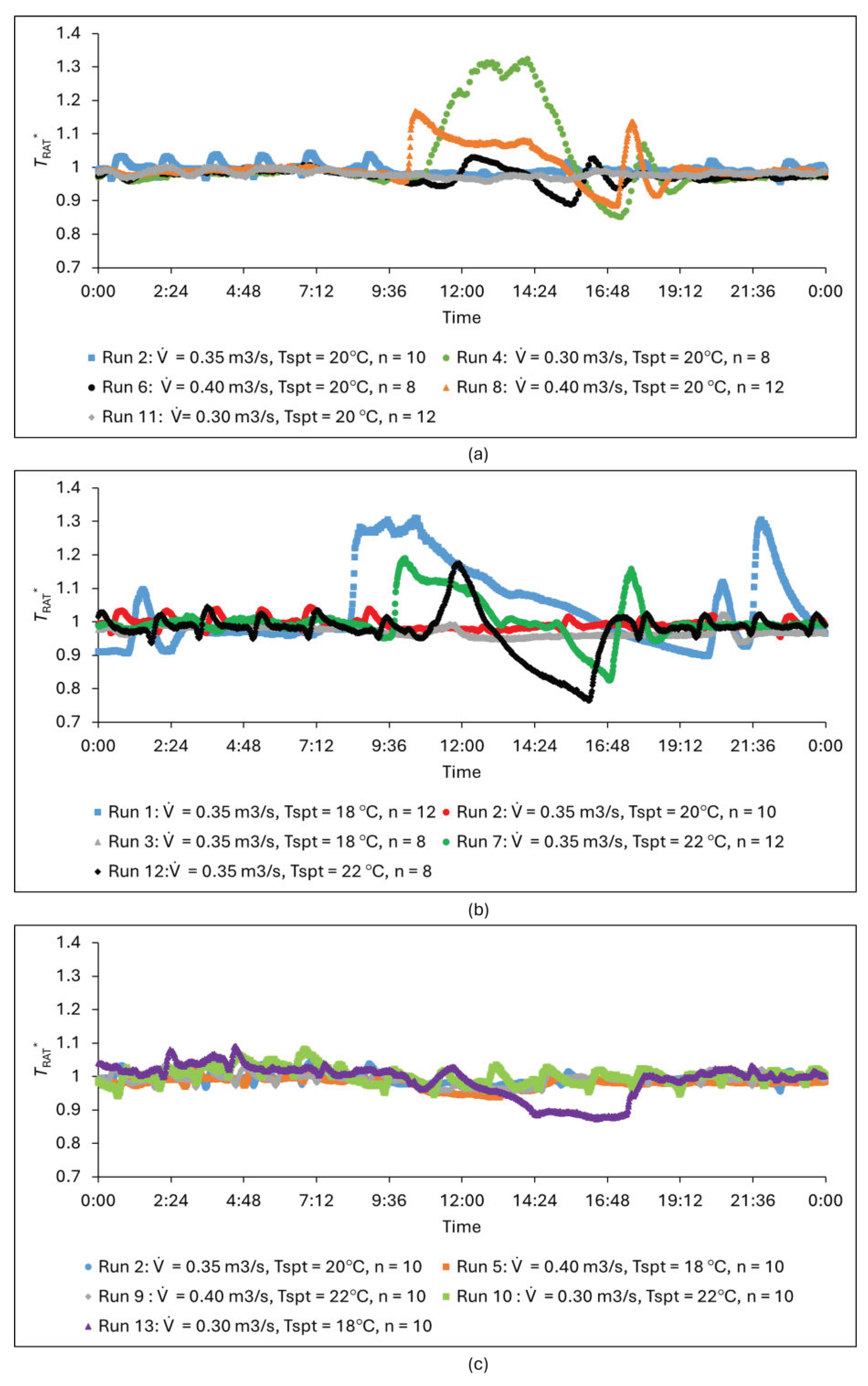
3.6.1. Dynamic Dimensionless Room Air Temperature (T_RAT^*) Profiles

Figure 13a–c show T_RAT^* the impact of three independent variables and the outdoor air temperature on the warm WCJ indoor air temperature within a greenhouse. Figure 13a shows the impact of $\dot{V}$ and n on T_RAT^*, with T_spt held constant at 20 °C. Figure 13b shows the effect of T_spt and n on T_RAT^* while maintaining $\dot{V}$ at 0.35 m³/s. Figure 13c shows the impact of $\dot{V}$ and T_spt on T_RAT^* with n at 10.

Figure 13a shows that at a given T_spt, T_RAT^* increases as n and $\dot{V}$ increase, as indicated by run 8. Runs 8 and 11 illustrate that a higher n results in a more uniform temperature. The stable indoor environment is associated with the increased shielding effect as n increases, allowing the WCJ to retain higher momentum and heat by limiting entrainment in Zones I and II. The warm WCJ supplied into the room induces a temperature rise by mixing with the cooler surrounding air, thus fostering a more homogeneous thermal environment. This effect is evident at a higher $\dot{V}$, as shown in run 8, and can be attributed to the turbulent nature of the WCJ, which enhances mixing and heat transfer with the surrounding air.

Figure 13b shows that at a specified $\dot{V}$, T_RAT^* rises with a higher T_spt, as illustrated by runs 7 and 12, but achieves a more stable indoor thermal environment at a lower T_spt, as shown in run 3. A lower T_spt leads to a denser WCJ, increasing the mass flow rate and enhancing the WCJ velocity and room air temperature uniformity. The T_RAT^* for run 3 is higher than run 1, demonstrating that decreasing n also raises T_RAT^* due to higher WCJ velocities, improving heat transfer and mixing with room air.

Figure 13c shows that a lower $\dot{V}$ and a higher T_spt, as seen in run 10, lead to non-uniform indoor air temperatures. Higher WCJ supply temperatures reduce jet density and mass flow rates, while larger temperature differences increase buoyancy effects. As a result, the WCJ mass flow and momentum of the WCJ decrease before reaching the occupied zone, limiting its ability to regulate room temperature. In contrast, decreasing T_spt at a lower $\dot{V}$ improves the air density and mass flow rate, enhancing WCJ performance and raising T_RAT^*, as demonstrated in run 13. This result confirms the result of a previous study [26].

Figure 13a–c demonstrate that the WCJ can meet any T_spt in heating mode, as T_RAT^* remains around 1. A T_RAT^* value below 1 indicates insufficient heating, while values above 1 suggest overheating, leading to potential energy waste. Due to solar radiation, runs 1, 4, 7, 8, and 12 show overheating (bulging profiles) between 10:00 AM and 15:00 PM. This is because of the solar irradiance, but the system was primarily configured for heating. So, switching to cooling mode was delayed, as the hot water in the buffer tank delayed reaching the required threshold for the supply air temperature. In Nordic climates, heating is needed even during the day, except when solar irradiance spikes. Therefore, active greenhouse heating occurs between 15:00 and 10:00 AM on days with sunny periods.

3.6.2. Contour Plots for Dimensionless Room Air Temperature (T_RAT^*)

The contour plots of T_RAT^* further illustrate the effect of the design variables on the indoor air temperature. Figure 14a shows the impact of $\dot{V}$ and n on T_RAT^*, with T_spt held constant at 20 °C. Figure 14b shows the effect of T_spt and n on T_RAT^* while maintaining $\dot{V}$ at 0.35 m³/s. Figure 14c shows the impact of $\dot{V}$ and T_spt on T_RAT^* with n at 10.

Figure 14a displays an increase in T_RAT^* as $\dot{V}$ and n rise due to the enhanced shielding effect of the inner jets of the confluent jet with a higher n. This flow behavior means the WCJ conserves and retains more thermal energy, impacting the room air temperature. At a lower $\dot{V}$, T_RAT^* tends to increase as n reduces.

Figure 14b shows T_RAT^* increasing with n at a lower T_spt, indicating that the thermal environment is affected by the jets’ shielding effect and the increased mass flow rate due to higher air densities.

Figure 14c shows that T_RAT^* rises as $\dot{V}$ and T_spt decrease, attributed to the higher air temperature supply at a lower $\dot{V}$, which influences the test room’s indoor thermal environment. To save energy, the WCJ can be supplied at low temperatures and $\dot{V}$ but still meet the required room air temperature. To optimize the influence of the WCJ on the room air temperature, a balance is required between $\dot{V}$ and T_spt since higher $\dot{V}$ and T_spt reduce T_RAT^*.

3.6.3. Response Surface Model for Dimensionless Room Air Temperature Correlations (T_RAT^*)

Equation (10) provides the regression equation of the response surface (RS) model, estimating the effects of the linear terms, quadratic terms, and two-way interaction terms of the design variables on T_RAT^*.

$$\begin{gathered} {T_{\mathrm{R}\mathrm{A}\mathrm{T}}}^{*}=1.17-0.023n+0.012T_{\mathrm{s}\mathrm{p}\mathrm{t}}-0.99\dot{V}+0.00089n\times n+0.00031T_{\mathrm{s}\mathrm{p}\mathrm{t}}\times T_{\mathrm{s}\mathrm{p}\mathrm{t}}-1.12\dot{V}\times \dot{V} \\ -0.00246 n\times T_{\mathrm{s}\mathrm{p}\mathrm{t}}+0.17n\times \dot{V}-0.002T_{\mathrm{s}\mathrm{p}\mathrm{t}}\times \dot{V} \end{gathered}$$

(10)

Equation (10) has an R² value of 60.5%, indicating a relatively good correlation. It shows that increasing $\dot{V}$ significantly decreases T_RAT^*, both linearly and quadratically. Increasing n also reduces T_RAT^* linearly, with a slight positive quadratic effect. The positive interaction between n and $\dot{V}$ suggests that a higher n can offset the negative impact of a higher $\dot{V}$. T_spt has a minor linear and quadratic effect, slightly increasing T_RAT^*, but its influence is less significant compared to $\dot{V}$.

Equations (7)–(10) are regression equations generated using MINITAB to represent the response surface model. These are second-order polynomials (quadratic model) that capture the influence of the interactions of n, T_spt, and $\dot{V}$, both individually and interactively, on the predicted dependent (response) variables. The sign (+ or -) and the value of the coefficients indicate the direction and magnitude of these effects, respectively. The R² values reflect the strengths of the correlations between the three design variables and each of the dependent variables (T_CST^*, T_EWT^*, T_SAT^*, and T_RAT^*), ranging from moderate to very strong. Moderate correlations are likely due to external factors like wind, solar radiation, and humidity, which were not accounted for in this study but can affect field measurements.

The response surface methodology gave the strengths of the influence of the three design variables on the WCJ with respect to T_CST^*, T_EWT^*, T_SAT^* and T_RAT^*.

Table 2. Strength of the effect of independent variables on the respective dependent variables.

Term	TCST*	TEWT*	TSAT*	TRAT*
Linear terms
n	V	IX	VI	II
Tspt	VI	II	II	V
$\dot{V}$	IV	I	I	IV
Quadratic terms
n × n	VII	V	V	VI
Tspt × Tspt	IX	VI	VIII	VIII
$\dot{V}$ × $\dot{V}$	VIII	IV	IX	VII
Two-way interactions terms
n × Tspt	II	VIII	III	III
n ×$\dot{V}$	I	III	IV	I
Tspt × $\dot{V}$	III	VII	VII	IX

shows the strength of the effects of the three design variables on the heating capacity of the WCJ on the ceiling, external wall, supply temperature, and room air temperature. The strength of influence is indicated by Roman numerals ranging from I, indicating a term with the strongest effect, to IX, for the term with the weakest influence.

The two-way interaction term between n and $\dot{V}$ exerts the strongest effect, whereas the quadratic term of T_spt has the least heating effect on T_CST^*. $\dot{V}$ had the highest effect, while n had the least effect on T_EWT^*. The linear term of $\dot{V}$ has the strongest effect, while the quadratic term of $\dot{V}$ has the least effect on T_SAT^*. The two-way interaction term between n and $\dot{V}$ had the most significant impact on T_RAT^*, while the interaction between T_spt and $\dot{V}$ had the least effect.

The airflow rate has the strongest effect on the capacity of the WCJ to heat the ceiling, external wall, and room air. Lowering the airflow rate boosted the WCJ heating effect on the ceiling but increased the supply temperature. Increasing the airflow rate improved the heating on the external wall and increased heat transfer into the room air when coupled with a higher number of nozzle rows. Lower airflow rates caused unstable room air temperature distribution. This result confirms the findings of a previous study that numerically investigated the airflow pattern and performance of wall confluent jet ventilation for heating in a typical office space. The study concluded that the WCJ supply velocity had a stronger effect on the jet velocity profile than the supply air temperature [76]. The number of nozzle rows had the moderate effect on the WCJ heating effect on the ceiling, external wall, and supply temperature.

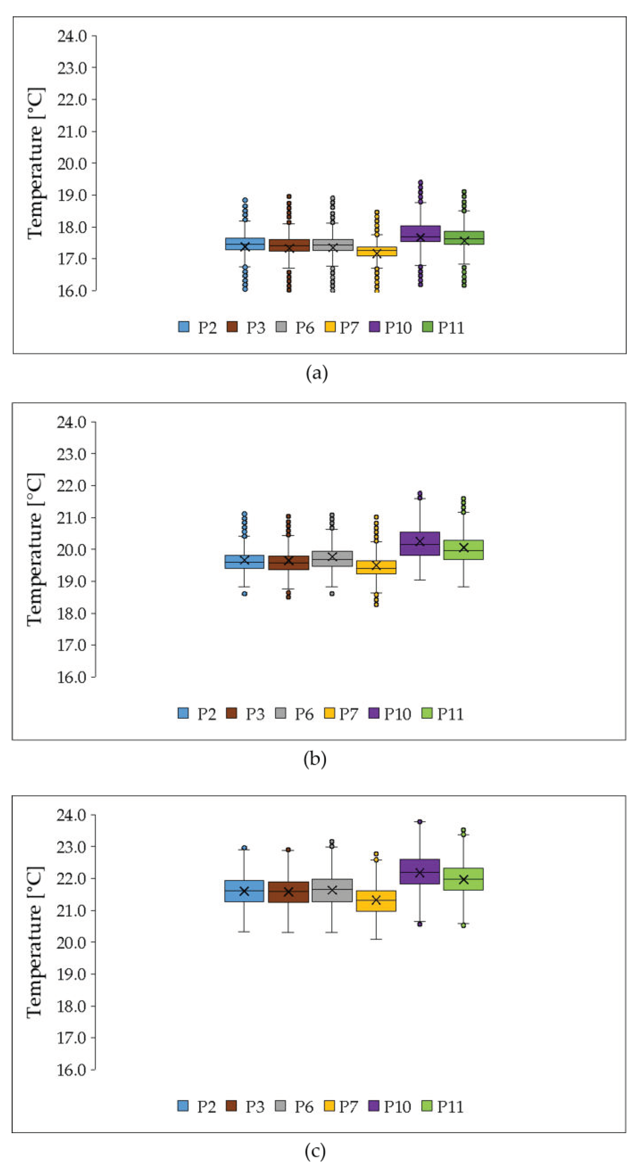
3.6.4. Room Air Temperature Distribution

The WCJ heats the cold ambient air, raising the room temperature to match T_spt. Figure 15 shows variations in the room air at various positions and heights in the test room. Representative runs 2, 5, and 9 have different room air setpoints and are selected for illustrative purposes. Figure 15a shows the air temperature distribution in the test room during run 5. Figure 15b shows the air temperature distribution in the test room during run 2. Figure 15c shows the air temperature distribution in the test room during run 9.

Figure 15a shows that the average room air temperature at 17.5 °C closely aligns with T_spt = 18 °C. The minimum and maximum temperatures were about 16.5 °C and 18.5 °C, respectively.

Figure 15b shows the air temperature in the test room is closer to 20 °C, which is the setpoint temperature for run 2. The air temperature varied between 19 °C and 20.5 °C, showing a marginal variability.

Figure 15c indicates the influence of the WCJ on raising the room air temperature to about 21.7 °C, closely matching the setpoint at 22 °C in run 9. This was despite the outdoor air temperature being −16.5 °C.

Figure 15 shows that the AHU system with the WCJ provided uniform temperatures close to each setpoint across runs, even with outdoor temperatures as low as −16.5 °C. Runs 2, 5, and 9 highlight stable temperature control (17° C to 24 °C) for various outdoor air temperatures that ranged from −16.5 °C to 3.1 °C. Although the difference is negligible, P6, P7, P10, and P11 indicate that temperatures at a height of 1.5 m are slightly higher than at 2.5 m due to the proximity of the WCJ, which flows closer to the floor. P10 and P11 record higher temperatures because they are placed near the external wall, where the WCJ first makes contact before moving to the floor. Positions P2 and P3 record slightly lower temperatures since they are farthest from the external wall, and the WCJ reaches them after losing significant heat. Lower room air temperature setpoints, such as run 5, are advantageous because they can save heating energy while providing the recommended air temperature. Across all the runs, the variation in room air temperature at different positions was negligible, indicating stable and uniform temperature distribution in the room. The minor variations indicate an effective, stable temperature distribution across the room, while occasional outliers reflect the heating system’s slower response to rapid outdoor air temperature changes. The results show that a WCJ diffuser with a total number of nozzle rows of n = 10, supplying a moderate airflow rate of 0.35 m³/s, provides adequate heating on a 7 m long ceiling adjoining to a 4 m high external wall and can create and maintain the room air temperature setpoint in a 6.6 m long room.

4. Further Discussion

The results of this study demonstrate that a warm WCJ can be used to climatize any greenhouse in a region that experiences outdoor air temperatures that fall within the range in this study.

The WCJ provides a strategy to provide space heating in greenhouses by applying a warm layer on the inner surfaces of the building envelope facades exposed to varying winter outdoor air temperature conditions. WCJ heating systems reduce primary energy demand in two ways. Firstly, the characteristic flow patterns enable the WCJ to retain the heat energy with which it is supplied into the occupied zone due to the shielding effect of the outer nozzles in the nozzle array. Although there are no comparative field studies to compare the WCJ heating capacity with other ventilation-based heating systems, prior studies show that WCJs have better energy efficiency than either displacement or mixing ventilation [44,47,76]. Secondly, to cost-effectively implement this strategy for space heating, the heating system should be connected to low-exergy heat sources (low-grade energy). This study recommends using cheaper heat sources such as industrial waste heat, heat from restaurants, and data centers, which would otherwise be released into the environment as waste heat. Low-exergy heat sources have temperatures near ambient (usually below 50 °C) and are hard to convert into other forms of energy (electricity) yet work well for applications requiring mild heating such as space heating. By harnessing low-exergy heat sources, greenhouse heating with wall confluent jet technology can reduce the demand for high-grade energy, conserve energy, and lower greenhouse gas emissions. Low-exergy energy sources serve as alternative heat sources that reduce the demand for primary energy generation, mitigating environmental pollution in the case of fossil fuel energy sources. The results of this study support and implement the findings from prior studies promoting low-exergy energy for space heating [77], enhanced energy efficiency, and sustainability in buildings and communities [78,79]. The results of this study present additional evidence of the possibility of using low-exergy heat sources to provide space heating in greenhouses, adding to a previous study that relied on exergy to operate heat pumps for heating greenhouses [80]. Additionally, the proposed heating method adds to the array of existing greenhouse heating technologies like water storage, phase change material storage, rock bed storage [81], and renewable energy sources [82]. The proposed WCJ heating system can be implemented in other large-space enclosures such as shopping and sports centers, airports, and railway stations in cold climates.

The results of this study benefit various stakeholders. They give greenhouse farmers knowledge of improved heating systems that reduce energy costs, enhance crop yields, and ensure stable temperatures for better plant growth, disease control, and extended growing seasons. HVAC engineers and manufacturers can leverage new data to develop more efficient air distribution systems for academic and agricultural research. Energy companies, environmental groups, governments, and policymakers can lobby for the design of energy-efficient diffusers and heating systems that promote sustainable development and reduce greenhouse gas emissions. Universities and research institutions can benefit from the insights for further studies, while governments and agricultural agencies can support policies aligning with energy-saving and food security goals. Agricultural researchers can apply the findings to optimize temperature control for increased productivity and sustainability in protected farming systems.

Further studies are required to assess the airflow patterns and temperature distribution in a greenhouse populated with live plants. More extended studies are needed to evaluate whether the heating system based on a WCJ can create a consistent indoor thermal environment to support plant growth through the growing stages of the plants in a stand-alone greenhouse. Further studies are required to connect excess industrial waste heat to greenhouse heating systems incorporating WCJ supply diffusers.

5. Conclusions

This study investigated the capacity of a warm wall confluent jet (WCJ) to regulate the climate in a greenhouse under dynamic meteorological conditions in winter. This study analyzed the effect of the airflow rate, number of nozzle rows, and room air temperature setpoint on the WCJ to heat the ceiling, external wall, and room air. The results show that the air distribution systems supplied the WCJ, which provided recommended air velocities and temperatures across all runs.

This study developed response surface models to correlate the independent design variables (n, $\dot{V}$, T_spt) with dependent variables like the room air temperature (T_RAT^*), the ceiling surface temperature (T_CST^*), the inner surface temperature of the external wall (T_EWT*), and the supply air temperature (T_SAT^*). These models provide practical insights for optimizing the performance of the WCJ heating system in greenhouses. A combination of a T_CST^* ranging from 0.95 to 1.1, a T_EWT^* of 0.8 to 0.95, and a T_SAT^* of 1.2 would give a T_RAT^* of about 1, indicating an optimum set indoor air temperature. The supply air temperature during the experiments ranged from 27 °C to 40 °C, indicating that low-exergy heat sources, such as industrial waste heat, can be effectively utilized in low-temperature heating systems integrated with WCJ supply diffusers to provide efficient heating for greenhouses.

The airflow rate has the strongest effect on the WCJ flow and thermal behavior along the ceiling, external wall, and room air. The number of nozzle rows had a moderate effect on the WCJ heating effect on the ceiling, external wall, and supply temperature. This study shows the potential application of WCJs in providing and sustaining recommended operational thermal conditions of greenhouses in winter. The results give insights into operational parameters to satisfy the conditions for greenhouses under varied winter meteorological conditions. To effectively heat the ceiling and external wall, an increase in the airflow rate should be accompanied by a corresponding increase in the number of nozzle rows. A WCJ diffuser with several nozzle rows supplying a moderate airflow rate provides adequate heating on the ceiling and external wall and can create and maintain the room air temperature setpoint. The WCJ supplied at lower airflow rates adequately heats the ceiling surface but provides insufficient heating on the external wall and room air. However, lowering both the airflow rates and room air temperature setpoints produces a WCJ that creates the required thermal environment coupled with some potential energy-saving benefits. This study shows that increasing the number of nozzles enhances the shielding effect, consequently augmenting the thermal sustenance of the insulation characteristics of the jet on building envelopes, especially the external wall, contributing to the required indoor thermal environment.

References

1. Oral, G.K.; Yilmaz, Z. Building form for cold climatic zones related to building envelope from heating energy conservation point of view. Energy Build. 2003, 35, 383–388. [Google Scholar] [CrossRef]
2. Pacheco, R.; Ordóñez, J.; Martínez, G. Energy efficient design of building: A review. Renew. Sustain. Energy Rev. 2012, 16, 3559–3573. [Google Scholar] [CrossRef]
3. Liu, X.; Lin, L.; Liu, X.; Zhang, T.; Rong, X.; Yang, L.; Xiong, D. Evaluation of air infiltration in a hub airport terminal: On-site measurement and numerical simulation. Build. Environ. 2018, 143, 163–177. [Google Scholar] [CrossRef]
4. Balaras, C.A.; Dascalaki, E.; Gaglia, A.; Droutsa, K. Energy conservation potential, HVAC installations and operational issues in Hellenic airports. Energy Build. 2003, 35, 1105–1120. [Google Scholar] [CrossRef]
5. Caruso, G.; De Santoli, L.; Mariotti, M. Ventilation Design in Large Enclosures for Sports Events using CFD: The Halls of the “Città dello Sport” in Rome. In Proceedings of the Clima 2007 WellBeing Indoors, Helsinki, Finland, 10–14 June 2007; pp. 1–10. [Google Scholar]
6. Calay, R.K.; Borresen, B.A.; Holdø, A.E. Selective ventilation in large enclosures. Energy Build. 2000, 32, 281–289. [Google Scholar] [CrossRef]
7. Von Elsner, B.; Briassoulis, D.; Waaijenberg, D.; Mistriotis, A.; Von Zabeltitz, C.; Gratraud, J.; Russo, G.; Suay-Cortes, R. Review of structural and functional characteristics of greenhouses in European Union countries: Part I, design requirements. J. Agric. Eng. Res. 2000, 75, 1–16. [Google Scholar] [CrossRef]
8. Briassoulis, D.; Waaijenberg, D.; Gratraud, J.; Von Eslner, B. Mechanical properties of covering materials for greenhouses: Part 1, general overview. J. Agric. Eng. Res. 1997, 67, 81–96. [Google Scholar] [CrossRef]
9. Badji, A.; Benseddik, A.; Bensaha, H.; Boukhelifa, A.; Hasrane, I. Design, technology, and management of greenhouse: A review. J. Clean. Prod. 2022, 373, 133753. [Google Scholar] [CrossRef]
10. Von Elsner, B.; Briassoulis, D.; Waaijenberg, D.; Mistriotis, A.; Von Zabeltitz, C.; Gratraud, J.; Russo, G.; Suay-Cortes, R. Review of structural and functional characteristics of greenhouses in European Union countries, part II: Typical designs. J. Agric. Eng. Res. 2000, 75, 111–126. [Google Scholar] [CrossRef]
11. Jeon, J.; Lee, J.; Ham, Y. Quantifying the impact of building envelope condition on energy use. Build. Res. Inf. 2019, 47, 404–420. [Google Scholar] [CrossRef]
12. Sozer, H. Improving energy efficiency through the design of the building envelope. Build. Environ. 2010, 45, 2581–2593. [Google Scholar] [CrossRef]
13. Manioğlu, G.; Yılmaz, Z. Economic evaluation of the building envelope and operation period of heating system in terms of thermal comfort. Energy Build. 2006, 38, 266–272. [Google Scholar] [CrossRef]
14. Al-Sanea, S.A.; Zedan, M.F.; Al-Hussain, S.N. Effect of thermal mass on performance of insulated building walls and the concept of energy savings potential. Appl. Energy 2012, 89, 430–442. [Google Scholar] [CrossRef]
15. Reilly, A.; Kinnane, O. The impact of thermal mass on building energy consumption. Appl. Energy 2017, 198, 108–121. [Google Scholar] [CrossRef]
16. Feng, G.; Sha, S.; Xu, X. Analysis of the building envelope influence to building energy consumption in the cold regions. Procedia Eng. 2016, 146, 244–250. [Google Scholar] [CrossRef]
17. Soytas, U.; Sari, R. Energy consumption, economic growth, and carbon emissions: Challenges faced by an EU candidate member. Ecol. Econ. 2009, 68, 1667–1675. [Google Scholar] [CrossRef]
18. Pérez-Lombard, L.; Ortiz, J.; Pout, C. A review on buildings energy consumption information. Energy Build. 2008, 40, 394–398. [Google Scholar] [CrossRef]
19. Yang, L.; Yan, H.; Lam, J.C. Thermal comfort and building energy consumption implications—A review. Appl. Energy 2014, 115, 164–173. [Google Scholar] [CrossRef]
20. Ortega Alba, S.; Manana, M. Energy research in airports: A review. Energies 2016, 9, 349. [Google Scholar] [CrossRef]
21. Lu, Y.; Dong, J.; Liu, J. Zonal modelling for thermal and energy performance of large space buildings: A review. Renew. Sustain. Energy Rev. 2020, 133, 110241. [Google Scholar] [CrossRef]
22. Palmowska, A.; Miczka, G. Research on the thermal conditions in ventilated large space building. ACEE J. 2018, 11, 169–178. [Google Scholar] [CrossRef]
23. Pérez-Lombard, L.; Ortiz, J.; Coronel, J.F.; Maestre, I.R. A review of HVAC systems requirements in building energy regulations. Energy Build. 2011, 43, 255–268. [Google Scholar] [CrossRef]
24. Barozzi, M.; Lienhard, J.; Zanelli, A.; Monticelli, C. The sustainability of adaptive envelopes: Developments of kinetic architecture. Procedia Eng. 2016, 155, 275–284. [Google Scholar] [CrossRef]
25. Kim, J.-J.; Moon, J.W. Impact of Insulation on Building Energy Consumption. In Proceedings of the Building Simulation, Glasgow, UK, 27–30 July 2009; Available online: https://www.aivc.org/resource/impact-insulation-building-energy-consumption (accessed on 13 October 2024).
26. Oral, G.K.; Yilmaz, Z. The limit U values for building envelope related to building form in temperate and cold climatic zones. Build. Environ. 2002, 37, 1173–1180. [Google Scholar] [CrossRef]
27. Elghamry, R.; Hassan, H. Impact of window parameters on the building envelope on the thermal comfort, energy consumption and cost and environment. Int. J. Vent. 2020, 19, 233–259. [Google Scholar] [CrossRef]
28. Asphaug, S.K.; Kvande, T.; Time, B.; Peuhkuri, R.H.; Kalamees, T.; Johansson, P.; Berardi, U.; Lohne, J. Moisture control strategies of habitable basements in cold climates. Build. Environ. 2020, 169, 106572. [Google Scholar] [CrossRef]
29. Ngirubiu, I.I. Circular Economy and Its Governance in Dutch Agri-Food Greenhouse Horticulture. Master’s Thesis, University of Twente, Enschede, The Netherlands, 2023. Available online: https://essay.utwente.nl/96769/ (accessed on 12 May 2024).
30. Aznar-Sánchez, J.A.; Velasco-Muñoz, J.F.; García-Arca, D.; López-Felices, B. Identification of opportunities for applying the circular economy to intensive agriculture in Almería (South-East Spain). Agronomy 2020, 10, 1499. [Google Scholar] [CrossRef]
31. Van Tuyll, A.; Boedijn, A.; Brunsting, M.; Barbagli, T.; Blok, C.; Stanghellini, C. Quantification of material flows: A first step towards integrating tomato greenhouse horticulture into a circular economy. J. Clean. Prod. 2022, 379, 134665. [Google Scholar] [CrossRef]
32. Torrellas, M.; Antón, A.; Ruijs, M.; Victoria, N.G.; Stanghellini, C.; Montero, J.I. Environmental and economic assessment of protected crops in four European scenarios. J. Clean. Prod. 2012, 28, 45–55. [Google Scholar] [CrossRef]
33. Martin, M.; Brandão, M. Evaluating the environmental consequences of Swedish food consumption and dietary choices. Sustainability 2017, 9, 2227. [Google Scholar] [CrossRef]
34. Critten, D.L.; Bailey, B.J. A review of greenhouse engineering developments during the 1990s. Agric. For. Meteorol. 2002, 112, 1–22. [Google Scholar] [CrossRef]
35. Vadiee, A.; Martin, V. Energy management strategies for commercial greenhouses. Appl. Energy 2014, 114, 880–888. [Google Scholar] [CrossRef]
36. Janbakhsh, S.; Moshfegh, B. Experimental investigation of a ventilation system based on wall confluent jets. Build. Environ. 2014, 80, 18–31. [Google Scholar] [CrossRef]
37. Awbi, H.B. Ventilation of Buildings; Routledge: London, UK, 2002. [Google Scholar]
38. Svensson, K. Experimental and Numerical Investigations of Confluent Round Jets; Linköping University Electronic Press: Linköping, Sweden, 2015; Available online: https://www.diva-portal.org/smash/record.jsf?dswid=667&pid=diva2%3A805327 (accessed on 24 January 2020).
39. Svensson, K.; Rohdin, P.; Moshfegh, B.; Tummers, M.J. Numerical and experimental investigation of the near zone flow field in an array of confluent round jets. Int. J. Heat Fluid Flow 2014, 46, 127–146. [Google Scholar] [CrossRef]
40. Ghahremanian, S. A Near-Field Study of Multiple Interacting Jets: Confluent Jets; Linkopings Universitet (Sweden): Linköping, Sweden, 2014. [Google Scholar] [CrossRef]
41. Karimipanah, T.; Awbi, H.B.; Blomqvist, C.; Sandberg, M.; Fresh, A.B. Effectiveness of confluent jets ventilation system for classrooms. In Proceedings of the 10th International Conference in Indoor Air Quality and Climate-Indoor Air, Beijing, China, 4–9 September 2005; Volume 5, pp. 3271–3277. [Google Scholar]
42. Andersson, H. Optimization of Confluent Jets Ventilation with Variable Airflow; Gävle University Press: Gävle, Sweden, 2022; Available online: https://www.diva-portal.org/smash/record.jsf?dswid=667&pid=diva2%3A1702356 (accessed on 3 June 2023).
43. Janbakhsh, S. A Ventilation Strategy Based on Confluent Jets: An Experimental and Numerical Study; Linköping University Electronic Press: Linköping, Sweden, 2015; Available online: https://www.diva-portal.org/smash/get/diva2:808188/FULLTEXT02.pdf (accessed on 23 September 2021).
44. Chen, H.; Janbakhsh, S.; Larsson, U.; Moshfegh, B. Numerical investigation of ventilation performance of different air supply devices in an office environment. Build. Environ. 2015, 90, 37–50. [Google Scholar] [CrossRef]
45. Choonya, G.; Larsson, U.; Moshfegh, B. Experimental investigations of flow and thermal behavior of wall confluent jets as a heating device for large-space enclosures. Build. Environ. 2023, 236, 110282. [Google Scholar] [CrossRef]
46. Arghand, T.; Karimipanah, T.; Awbi, H.B.; Cehlin, M.; Larsson, U.; Linden, E. An experimental investigation of the flow and comfort parameters forunder-floor, confluent jets and mixing ventilation systems in an open-plan office. Build. Environ. 2015, 92, 48–60. [Google Scholar] [CrossRef]
47. Karimipanah, T.; HB, A.; Moshfegh, B. The air distribution index as an indicator for energy consumption and performance of ventilation systems. J. Hum.-Environ. Syst. 2008, 11, 77–84. [Google Scholar] [CrossRef]
48. Janbakhsh, S.; Moshfegh, B. Numerical study of a ventilation system based on wall confluent jets. HVAC&R Res. 2014, 20, 846–861. [Google Scholar]
49. Cho, Y.; Awbi, H.B.; Karimipanah, T. Theoretical and experimental investigation of wall confluent jets ventilation and comparison with wall displacement ventilation. Build. Environ. 2008, 43, 1091–1100. [Google Scholar] [CrossRef]
50. Swedish Meteorological and Hydrological Institute. Climate Indicator-Temperature|SMHI. SMHI. Available online: https://www.smhi.se/en/climate/climate-indicators/climate-indicators-temperature-1.91472 (accessed on 5 December 2024).
51. Hoforsbacken, D.; Observation, S. LÄGSTA UPPMÄTTA TEMPERATURER, HOFORS. Available online: https://www.vackertvader.se/väderstation/hoforsbacken (accessed on 4 December 2024).
52. Fatnassi, H.; Boulard, T.; Benamara, H.; Roy, J.C.; Suay, R.; Poncet, C. Increasing the height and multiplying the number of spans of greenhouse: How far can we go? Acta Hortic. 2017, 1170, 137–143. [Google Scholar] [CrossRef]
53. EN 60751; Industrial Platinum Resistance Thermometers and Platinum Temperature Sensors. European Committee for Standardization (CEN)/CENELEC: Brussels, Belgium, 2008.
54. Montgomery, D.C. Design and Analysis of Experiments; John Wiley & Sons: Hoboken, NJ, USA, 2017. [Google Scholar]
55. Box, G.E.P.; Behnken, D.W. Some new three level designs for the study of quantitative variables. Technometrics 1960, 2, 455–475. [Google Scholar] [CrossRef]
56. Box, G.E.P.; Behnken, D.W. Simplex-sum designs: A class of second order rotatable designs derivable from those of first order. Ann. Math. Stat. 1960, 31, 838–864. [Google Scholar] [CrossRef]
57. Svensson, K.; Rohdin, P.; Moshfegh, B. A computational parametric study on the development of confluent round jet arrays. Eur. J. Mech. 2015, 53, 129–147. [Google Scholar] [CrossRef]
58. Andersson, H.; Cehlin, M.; Moshfegh, B. An investigation concerning optimal design of confluent jets ventilation with variable air volume. Int. J. Vent. 2023, 23, 183–203. [Google Scholar] [CrossRef]
59. Abad, M.; Monteiro, A.A. The use of auxins for the production of greenhouse tomatoes in mild-winter conditions: A review. Sci. Hortic. 1989, 38, 167–192. [Google Scholar] [CrossRef]
60. Peet, M.M.; Welles, G.W.H. Greenhouse tomato production. Crop Prod. Sci. Hortic. 2005, 13, 257. [Google Scholar]
61. Myers, R.H.; Montgomery, D.C.; Anderson-Cook, C.M. Response Surface Methodology: Process and Product Optimization Using Designed Experiments; John Wiley & Sons: Hoboken, NJ, USA, 2016. [Google Scholar]
62. Khuri, A.I.; Mukhopadhyay, S. Response surface methodology. Wiley Interdiscip. Rev. Comput. Stat. 2010, 2, 128–149. [Google Scholar] [CrossRef]
63. Khuri, A.I.; Cornell, J.A. Response Surfaces: Designs and Analyses: Revised and Expanded; CRC Press: Boca Raton, FL, USA, 2018. [Google Scholar]
64. Mäkelä, M. Experimental design and response surface methodology in energy applications: A tutorial review. Energy Convers. Manag. 2017, 151, 630–640. [Google Scholar] [CrossRef]
65. Myers, R.H.; Montgomery, D.C.; Vining, G.G.; Borror, C.M.; Kowalski, S.M. Response surface methodology: A retrospective and literature survey. J. Qual. Technol. 2004, 36, 53–77. [Google Scholar] [CrossRef]
66. Blackburn, T.D. Six Sigma: A Case Study Approach Using Minitab®; Springer Nature: Berlin/Heidelberg, Germany, 2022. [Google Scholar]
67. Gupta, B.C. Statistical Quality Control: Using MINITAB, R, JMP and Python; John Wiley & Sons: Hoboken, NJ, USA, 2021. [Google Scholar]
68. Evans, M. Minitab Manual; University of Toronto: Toronto, ON, Canada, 2009; ISBN 0-7167-2994-6. [Google Scholar]
69. Eldeeb, A. Adoption of Lean Six Sigma Using Minitab Software to Improve Industries Performance. Ph.D. Thesis, Hochschule für Technik und Wirtschaft Berlin, Berlin, Germany, 2023. [Google Scholar]
70. Bruun, H.H. Hot-wire anemometry: Principles and signal analysis. Meas. Sci. Technol. 1996, 7, 24. [Google Scholar] [CrossRef]
71. Lomas, C.G. Fundamentals of Hot Wire Anemometry; Cambridge University Press: Cambridge, UK, 2011. [Google Scholar]
72. Duff, M.; Towey, J. Two ways to measure temperature using thermocouples feature simplicity, accuracy, and flexibility. Analog Dialogue 2010, 44, 1–6. [Google Scholar]
73. Choonya, G.; Larsson, U.; Moshfegh, B. Heating of Cold Wall with Confluent Jets in Large Space Enclosures: Application in Greenhouse Premises. In Proceedings of the International Conference on Building Energy and Environment; Springer: Berlin/Heidelberg, Germany, 2022; pp. 1925–1933. [Google Scholar]
74. Wheeler, E.F.; Both, A.J. Evaluating Greenhouse Mechanical Ventilation System Performance, Part 3 of 3; The State University of New Jersey Rutgers Cooperative Extension: New Brunswick, NJ, USA, 2002. [Google Scholar] [CrossRef]
75. Holder, R.; Cockshull, K.E. Effects of humidity on the growth and yield of glasshouse tomatoes. J. Hortic. Sci. 1990, 65, 31–39. [Google Scholar] [CrossRef]
76. Tan, D.; Li, B.; Cheng, Y.; Liu, H.; Chen, J. Airflow pattern and performance of wall confluent jets ventilation for heating in a typical office space. Indoor Built Environ. 2020, 29, 67–83. [Google Scholar] [CrossRef]
77. Rosen, M.A.; Dincer, I.; Kanoglu, M. Role of exergy in increasing efficiency and sustainability and reducing environmental impact. Energy Policy 2008, 36, 128–137. [Google Scholar] [CrossRef]
78. Dincer, I.; Rosen, M.A. Energy, environment and sustainable development. Appl. Energy 1999, 64, 427–440. [Google Scholar] [CrossRef]
79. Schmidt, D. Low exergy systems for high-performance buildings and communities. Energy Build. 2009, 41, 331–336. [Google Scholar] [CrossRef]
80. Hepbasli, A. A comparative investigation of various greenhouse heating options using exergy analysis method. Appl. Energy 2011, 88, 4411–4423. [Google Scholar] [CrossRef]
81. Sethi, V.P.; Sharma, S.K. Survey and evaluation of heating technologies for worldwide agricultural greenhouse applications. Sol. Energy 2008, 82, 832–859. [Google Scholar] [CrossRef]
82. Esen, M.; Yuksel, T. Experimental evaluation of using various renewable energy sources for heating a greenhouse. Energy Build. 2013, 65, 340–351. [Google Scholar] [CrossRef]
Figure 1. Wall confluent jet (WCJ) characteristic velocity and temperature profiles. Note, Ub is inlet bulk velocity, Tin is inlet temperature, Twall is wall surface temperature, Umax is maximum streamwise velocity, Umax0.5 is half of the maximum streamwise velocity, x is distance from external cold wall, x0.5 is distance from external cold wall at which maximum streamwise velocity becomes half, and z is distance from WCJ supply device [45].
Energies 17 06217 g001
Figure 2. (a) Picture of the installed WCJ diffuser and supply air duct; (b) WCJ diffuser nozzle plate with representative nozzles. Note: d is diameter of nozzle, E is spacing between adjacent nozzles, w is width of nozzle plate, l is length of nozzle plate, n is number of nozzle rows, and m is number of nozzle columns.
Energies 17 06217 g002
Figure 3. Schematic diagram of the HVAC system for the test room.
Energies 17 06217 g003
Figure 4. Side view of the test room showing zones for WCJ velocity and temperature measurement, room air temperature measurement positions, and a picture of the front view of the test room. Note: A, B, and C are zoomed-in views showing the orientation of constant current anemometers. D is a picture of the front view of the test room. P1, P4, P5, P8, P9, and P12 are measurement positions for WCJ velocity and temperature using constant current anemometers. P2, P3, P6, P7, P10, and P11 are measurement positions for room air temperature using thermocouples, and Tspt is the room air temperature setpoint using the PT100 temperature sensor.
Energies 17 06217 g004
Figure 5. WCJ velocity: (a) average WCJ velocity at P12 in Zone I, (b) WCJ velocity distribution at P12 in Zone I, (c) average WCJ velocity at different heights along the inner surface of the external wall in Zone II, (d) WCJ velocity distribution at H = 2.7 in Zone II, (e) average velocity at different points along the floor in Zone III, and (f) WCJ velocity distribution at P5 in Zone III.
Energies 17 06217 g005
Figure 6. WCJ temperature: (a) average WCJ temperature at P12 in Zone I, (b) WCJ temperature distribution at P12 in Zone I, (c) average WCJ temperature at different heights along the inner surface of the external wall in Zone II, (d) WCJ temperature distribution at H = 2.7 in Zone II, (e) average temperature at different points along the floor in Zone III, and (f) WCJ temperature distribution at P5 in Zone III.
Energies 17 06217 g006
Figure 7. Dimensionless ceiling surface temperature (TCST*) profiles for 24 h: (a) for room air temperature setpoint (Tspt) = 20 °C, (b) for airflow rate ( V ˙ ) = 0.35 m3/s, and (c) the number of nozzle rows (n) = 10. Note: T C S T * = T c s t T o u t T s p t T o u t ; z is the distance from WCJ diffuser.
Energies 17 06217 g007
Figure 8. Contour plots showing the interaction between two design variables while holding the third variable on the mid-level value on the dimensionless ceiling surface temperature (TCST*): (a) airflow rate ( V ˙ ) vs. number of nozzle rows (n); (b) room air temperature setpoint (Tspt) vs. number of nozzle rows (n); and (c) airflow rate ( V ˙ ) vs. room air temperature setpoint (Tspt). Note: TCST* = T C S T * = T c s t T o u t T s p t T o u t and Tspt = Tspt.
Energies 17 06217 g008
Figure 9. Dimensionless inner surface temperature of the external wall (TEWT*) profiles for over 24 h: (a) room air temperature setpoint (Tspt) = 20 °C, (b) airflow rate ( V ˙ ) = 0.35 m3/s, and (c) number of nozzle rows (n) = 10. Note: T E W T * = T e w t T o u t T s p t T o u t ; H is the height above the floor.
Energies 17 06217 g009
Figure 10. Contour plots of the interaction between two design variables while holding the third variable on the mid-level value on the dimensionless inner surface temperature of the external wall (TEWT*): (a) airflow rate ( V ˙ ) vs. number of nozzle rows (n); (b) room air temperature setpoint (Tspt) vs. number of nozzle rows (n); and (c) airflow rate ( V ˙ ) vs. room air temperature setpoint (Tspt). Note: TEWT* = T E W T * = T e w t T o u t T s p t T o u t and Tspt = Tspt.
Energies 17 06217 g010
Figure 11. Dimensionless supply air temperature (TSAT*) profiles for 24 h: (a) room air temperature setpoint (Tspt) = 20 °C, (b) flow rate ( V ˙ ) = 0.35 m3/s, (c) number of nozzle rows (n) = 10. Note: T S A T * = T s a t T o u t T s p t T o u t .
Energies 17 06217 g011
Figure 12. Contour plots of the interaction between two design variables while holding the third variable on the mid-level value on the dimensionless inner surface temperature of the external wall (TSAT*): (a) airflow rate ( V ˙ ) vs. number of nozzle rows (n); (b) room air temperature setpoint (Tspt) vs. number of nozzle rows (n); and (c) airflow rate ( V ˙ ) vs. room air temperature setpoint (Tspt). Note: TSAT* = T S A T * = T s a t T o u t T s p t T o u t and Tspt = Tspt.
Energies 17 06217 g012
Figure 13. Dimensionless room air temperature (TRAT*) profiles for 24 h: (a) room air temperature setpoint (Tspt) = 20 °C, (b) airflow rate ( V ˙ ) = 0.35 m3/s, and (c) the number of nozzle rows (n) = 10. Note: T R A T * = T r a t T o u t T s p t T o u t .
Energies 17 06217 g013
Figure 14. Contour plots of the interaction between two design variables while holding the third variable on the mid-level value on the dimensionless room air temperature TRAT*: (a) airflow rate ( V ˙ ) vs. number of nozzle rows (n); (b) room air temperature setpoint (Tspt) vs. number of nozzle rows (n); and (c) airflow rate ( V ˙ ) vs. room air temperature setpoint (Tspt). Note: TRAT* = T R A T * = T r a t T o u t T s p t T o u t   and Tspt = Tspt.
Energies 17 06217 g014
Figure 15. (a) Room air temperature distribution in the test room during run 5: V ˙ = 0.40 m3/s, Tspt = 18 °C, n = 10; (b) room air temperature distribution in the test room during run 2: V ˙ = 0.35 m3/s, Tspt = 20 °C, n = 10and (c) room air temperature distribution in the test room during run 9: V ˙ = 0.40 m3/s, Tspt = 22° C, n = 10.
Energies 17 06217 g015