ML-Enabled Solar PV Electricity Generation Projection for a Large Academic Campus to Reduce Onsite CO₂ Emissions

Abstract

Mitigating CO₂ emissions is essential to reduce climate change and its adverse effects on ecosystems. Photovoltaic electricity is 30 times less carbon-intensive than coal-based electricity, making solar PV an attractive option in reducing electricity demand from fossil-fuel-based sources. This study looks into utilizing solar PV electricity production on a large university campus in an effort to reduce CO₂ emissions. The study involved investigating 153 buildings on the campus, spanning nine years of data, from 2015 to 2023. The study comprised four key phases. In the first phase, PVWatts gathered data to predict PV-generated energy. This was the foundation for Phase II, where a novel tree-based ensemble learning model was developed to predict monthly PV-generated electricity. The SHAP (SHapley Additive exPlanations) technique was incorporated into the proposed framework to enhance model explainability. Phase III involved calculating historical CO₂ emissions based on past energy consumption data, providing a baseline for comparison. A meta-learning algorithm was implemented in Phase IV to project future CO₂ emissions post-solar PV installation. This comparison estimated a potential emissions reduction and assessed the university’s progress toward its net-zero emissions goals. The study’s findings suggest that solar PV implementation could reduce the campus’s CO₂ footprint by approximately 18% for the studied cluster of buildings, supporting sustainability and cleaner energy use on the campus.

1. Introduction

In 2023, the United States generated approximately 4.18 trillion kilowatt hours (kWh) of electricity [1]. Approximately 60% of the total electricity generation was derived from fossil fuels such as coal, natural gas, and petroleum. Nuclear energy contributed about 19% of the overall electricity generation, while renewable energy sources, such as wind (10.4%), solar (3.9%), hydropower (5.7%), biomass (1.10%), and geothermal and other sources (0.5%) accounted for approximately 21% of the total electricity generated, as depicted in Figure 1. The United States aims to achieve a 100% carbon-free power system by 2035 and a net-zero-emissions energy economy by 2050. To reach this goal, pathways for integrating renewable power sources into the energy system must be identified [2,3,4]. Low-carbon technologies such as solar and wind are well positioned for cost-effective deployment at a larger scale. This aligns with previous technical and economic assessments indicating the potential for a rapid transformation of the U.S. power system and with widespread electrification across various sectors of the economy [5].

The combined end-use energy consumption from the residential and commercial sectors constituted approximately 27.6% of total U.S. end-use energy consumption, equivalent to about 20.6 quadrillion Btu [5]. Buildings are the biggest electricity consumers globally, consuming about 40% to 60% of a nation’s total energy consumption [6]. Heating, ventilation, and air conditioning systems (HVAC) are residential and commercial buildings’ most significant energy consumers. Within buildings, water heating, space heating, and space cooling account for 48.7% of the building’s primary energy consumption [7,8]. Electric resistance heaters and heat pumps have been proposed for space and water heating as part of decarbonization initiatives. Swift migration to electric heating while carbon-neutral electricity generation is still expanding may not reduce primary energy consumption and CO₂ emissions to the required levels [9]. Shifting away from fossil-fuel-based equipment to electric counterparts reduces onsite CO₂ emissions; however, the shift toward electrification for all of a facility’s needs can compromise the existing electrical infrastructure [10]. As electricity usage continues to increase, the electric grid must adapt to ensure the delivery of economically competitive and reliable electricity. The transition toward electrification will necessitate significant changes in grid infrastructure, operations, and planning to meet future demands [11].

The key to urban built environment decarbonization technologies includes sustainable and feasible renewable sources of electricity generation, such as rooftop solar PV [12,13]. The rapid deployment of photovoltaic (PV) technologies worldwide has decreased the price of PV systems [14]. Solar PV systems installed on rooftops are the most preferred option among least invasive renewable energy (LIRE) solutions due to the growing scarcity of natural lands [15]. In light of the growing efficiencies of rooftop solar PV and the lower price of PV systems, the number of rooftop solar PV installations has increased in the last decade. Solar PV systems can help supplement a considerable portion of the building’s electrical power demand if designed appropriately. However, the solar irradiance incident on the panels is contingent on multiple factors and is naturally intermittent and unpredictable [16]. To alleviate this intermittency, in the last decade, the focus has increased on managing the demand-side energy usage of facilities. By controlling the demand during peak hours, facilities can manage the balance between consumption and generation by reducing the effects of peak demand charges and maximizing the energy generated by solar PV. Programs that reduce a utility’s peak demand, such as high-efficiency HVAC demand-side management programs, generally hold higher value for utilities than other options [17]. To reduce peak demand, make better use of energy onsite, and reduce onsite CO₂ emissions, facilities are being pushed to install energy storage systems [18]. Energy storage systems allow facilities to store surplus energy when demand is low and release it during peak periods, thereby maximizing efficiency and reducing peak demand while contributing to overall grid stability. As policies and technologies evolve, the integration of energy storage becomes crucial for facilities aiming to meet both operational and environmental targets.

The primary objective of this study is to predict and analyze the effect of solar PV implementation on CO₂ emissions using advanced machine learning techniques. By leveraging data from the buildings on the University of Maryland campus, this research aims to develop robust models that can accurately forecast PV-generated energy and its subsequent effect on reducing greenhouse gas emissions. The goal is to provide valuable insights for long-term sustainability planning and to inform policy-making processes.

This project was structured into four phases, each contributing to the overall objective. In Phase I, extensive data were prepared to ensure a robust dataset. This process included filtering incomplete records and gathering relevant features such as the roof area, site area, and solar radiation data. Phase II involved implementing and evaluating various models, including linear regression, lasso regression, gradient boosting, random forest, decision trees, and neural networks. Tree-based models showed superior performance compared to other options. In Phase III, historical CO₂ emissions were analyzed for the years 2015–2022 to determine the baseline for the final phase. Finally, in Phase IV, the model was used to project future emissions using forecasted input features and ensemble learning. The study demonstrates the effectiveness of solar PV implementation in reducing CO₂ emissions in the long term; it also demonstrates how machine learning can streamline the prediction process.

2. Review of State-of-the-Art Methodologies

Recent studies have made significant progress in solar PV power forecasting using various machine learning techniques, including ensemble methods, probabilistic models, hierarchical approaches, and deep learning. These works emphasize the importance of model optimization and interpretability in improving prediction accuracy. The following section discusses related studies that focus on improving long-term and short-term solar PV power forecasting through advanced machine learning techniques.

2.1. Enhancing PV Power Forecasting with Deep Learning and Optimizing Solar PV Project Performance with Economic Viability: A Multi-Case Analysis of 10 MW Masdar Project in UAE [19]

This work presents a comprehensive study on the prediction of solar photovoltaic (PV) power generation using various machine learning algorithms. These algorithms include ensemble regression trees (ERTs), support vector machines (SVMs), Gaussian process regression (GPR), and artificial neural networks (ANNs). The authors enhance the performance of these algorithms through hyperparameter optimization using Bayesian optimization and random search techniques. The study utilizes hourly data with a 30 min resolution collected over a year from a 10 MW Masdar solar PV project in the United Arab Emirates (UAE). The results indicated that GPR, which was optimized using Bayesian optimization, outperforms other algorithms in terms of prediction accuracy, followed by ANN, ERT, and SVM. The paper underscores the importance of hyperparameter optimization in improving ML model performance and highlights the impact of this optimization on the adaptability and accuracy of solar PV power predictions under varying seasonal conditions. Through five case studies, this research identified optimal configurations for solar PV systems. Key findings included the best performance settings: a tilt angle of 20°, a ground coverage ratio (GCR) of 0.1, and a tracking rotation of 60°, which resulted in improved financial outcomes. The authors also provide insights into the UAE’s renewable energy transition, emphasizing the role of solar energy in meeting future energy demands [19]. In the current research, a tree-based ensemble learning approach, similar to the ensemble regression trees (ERT) applied in the Masdar project, was adopted to predict PV-generated energy. Building on this study’s emphasis on seasonal variability in solar PV performance, the present work also addresses monthly variations in solar energy output, which enhances the reliability of the long-term prediction model. This research uses advanced machine learning and hyperparameter optimization to enhance solar PV power forecasting and identify optimal configurations for better economic and energy performance.

2.2. Day-Ahead Regional Solar Power Forecasting with Hierarchical Temporal Convolutional Neural Networks Using Historical Power Generation and Weather Data [20]

This study presents novel deep-learning methods for predicting regional solar power generation. The authors proposed two hierarchical temporal convolutional neural network (HTCNN) architectures designed to handle both aggregated and individual power generation time series along with weather data. The methods were evaluated using data from 101 locations in Western Australia. The results demonstrated superior accuracy over traditional forecasting models such as long short-term memory (LSTMs) and convolutional neural networks (CNNs). The hierarchical approach, particularly when regions are divided into sub-regions based on weather conditions, significantly improved forecast accuracy, achieved a forecast skill score of 40.2%, and reduced forecast error by 6.5% compared to the best-performing benchmarks. This research underscores the importance of incorporating detailed weather data and hierarchical modeling for accurate regional solar power forecasting. This is crucial for managing electricity supply and demand in grids with high levels of distributed solar generation. However, one of the drawbacks of this study is the need to retrain the model from scratch whenever new data, such as the installation of additional PV systems, becomes available. This can lead to potential elevated costs and delays in model updates. The focus of this study on hierarchical modeling for regional solar power forecasting aligns with the current work in terms of its emphasis on improving forecasting accuracy through advanced machine learning techniques. Both approaches utilize weather and historical power generation data to predict solar energy output while taking different paths [20]. This research presents hierarchical temporal convolutional neural networks (HTCNNs) that combine aggregated and individual power generation data with weather information, resulting in improved accuracy in regional solar power forecasting through weather-based region subdivisions.

2.3. An Interpretable Probabilistic Model for Short-Term Solar Power Forecasting Using Natural Gradient Boosting [21]

This work introduced a two-stage probabilistic forecasting framework that combined natural gradient boosting (NGBoost) with Shapley additive explanations (SHAP) for short-term solar power prediction. The first stage used NGBoost to generate accurate and reliable probabilistic forecasts, while the second stage employed SHAP values to interpret the model’s predictions and provided transparency and insights into feature interactions and their impact on the predictions. The model was validated using data from two PV parks in southern Germany, and it demonstrated superior performance in both point and probabilistic forecasts compared to the Gaussian process and lower upper bound estimation methods. The study emphasizes the importance of interpretability in machine learning models for critical applications like power system operations, and it highlights how these models can help increase trust, detect biases, and enhance decision-making processes in the energy sector [21]. The model’s capacity to identify and utilize significant features leads to enhanced performance metrics, evidenced by a 6% reduction in RMSE and a 10% increase in Continuous Ranked Probability Score (CRPS). Both approaches emphasize the importance of transparency and interpretability in machine learning models for energy forecasting, while the method of the present study emphasizes long-term solutions. This research innovatively combines natural gradient boosting (NGBoost) with Shapley additive explanations (SHAP), yielding accurate probabilistic forecasts and enhanced interpretability. This integration improves transparency and trust while providing insights essential for short-term solar power forecasting.

2.4. A Comprehensive Framework for Effective Long Short-Term Solar Yield Forecasting [22]

This study introduced a novel framework that integrates machine learning techniques, which include XGBoost (version is 2.0.3), time series seasonal decomposition, and rolling LSTM, to forecast solar photovoltaic (PV) output for both short and long-term durations. The framework was designed to enhance the accuracy and reliability of PV yield predictions, thereby facilitating better integration with the main power grid. The proposed model demonstrates high prediction accuracy (98–95%) and forecasting accuracy (89–87%), outperforming existing models in terms of error metrics such as normalized root mean square error (nRMSE). This comprehensive approach addressed the need for an automated input feature selection and data cleaning, making it a robust tool for managing the variability of solar power generation in diverse climatic conditions [22]. Both methods emphasized long-term forecasting, while the present study also conducts a detailed analysis of the impact of solar PV on CO₂ emissions.

The present research builds upon these foundational studies by incorporating a tree-based ensemble learning model that integrates insights from both model optimization and interpretability. Similar to the referenced works, this study aims to enhance prediction accuracy and robustness, particularly within the realm of long-term solar PV power forecasting. By employing advanced techniques such as SHAP analysis and meta-learning, the current research aims to further advance the development of reliable forecasting models, with a particular emphasis on solar PV implementation to achieve long-term reductions in CO₂ emissions. The present research presents a novel framework that combines advanced machine learning techniques, such as XGBoost, decision tree, and random forest, to accurately forecast long-term solar PV yields while automating feature selection and data cleaning for robustness across different climatic conditions.

The paper introduces two significant novel contributions that set it apart from existing research on machine learning applications in photovoltaic (PV) systems. The first contribution is the integration of emission studies with predictions of PV-generated energy. This dual-focus approach effectively bridges the gap between energy modeling and environmental impact assessment, offering valuable insights into the role of solar PV systems in mitigating CO₂ emissions. By quantifying these reductions alongside energy forecasts, the study creates a comprehensive framework that simultaneously addresses energy efficiency and sustainability objectives—an area often considered separately in previous research.

The second noteworthy innovation is the implementation of a monthly validation methodology. Unlike traditional cross-validation techniques that average model performance across the entire dataset, monthly validation evaluates the performance of predictive models on a month-by-month basis. This method considers seasonal variability in solar energy generation, which is crucial for precise modeling in photovoltaic (PV) systems. By establishing monthly validation as the cornerstone for ensemble learning models, the study ensures that the unique characteristics of each month’s data are acknowledged, resulting in more robust and reliable predictions. These advancements render the study a significant contribution to the literature, providing actionable insights for energy planning and environmental impact mitigation.

3. Research Methodology

This section provides a discussion of the study’s four key phases: data preparation, tree-based ensemble learning model to predict PV-generated energy, analyzing the impact of PV-generated energy on CO₂ Emissions (2015–2022), and predicting the future impact of Solar PV on CO₂ emissions. A flowchart of the research methodology is provided in Figure 2.

3.1. Phase I: Data Preparation

In Phase I, the primary focus was on preparing and organizing data for subsequent analyses. The initial dataset contained energy data for 200 buildings within the University of Maryland’s campus. The first step involved refining the dataset by excluding buildings and finding outliers with incomplete utility bills, which resulted in a final dataset of 153 buildings.

For each building, various features were collected to create a suitable dataset. The roof area was obtained using Google Earth [23], while the site area and energy consumption details were extracted from TerpFootprint [24], a tool that provides and manages utility bill data for the University of Maryland campus buildings. Solar radiation features, including global horizontal irradiance (GHI), direct normal irradiance (DNI), diffuse horizontal irradiance (DHI), and weather-related features, such as wind speed and temperature, were collected from the National Solar Radiation Database (NSRDB) [25].

To estimate the photovoltaic (PV)-generated energy, an open-source tool developed by the National Renewable Energy Laboratory (NREL), PVWatts [26], was utilized. This tool calculates monthly and annual AC energy generation based on location, system size, type of array, tilt angle, azimuth angle, and other parameters. For this analysis, after a few trials and errors, 50% of the roof area was considered for potential solar PV installation. Research conducted by organizations such as NREL reveals that, on average, commercial buildings with flat roofs can utilize about 50% of their roof area for solar energy generation [27]. It is presumed that all electricity produced by the rooftop photovoltaic (PV) array would be used to offset the facility’s electricity consumption. This assumption is based on the observation that commercial office buildings typically have high electricity usage during daylight hours, which coincides with peak solar PV energy generation. This highlights the significant potential for effectively harnessing solar power in these settings. By generating renewable energy onsite, facilities can reduce their reliance on the grid [28]. Installing solar PV systems on 50% of roof areas is economically viable for many buildings, particularly since the cost-effectiveness of rooftop PV systems has improved considerably in recent years. The decline in solar panel prices, along with incentives such as tax credits and rebates, makes investing in rooftop solar installations not only practical but also attractive to building owners.

Following the data preparation, separate datasets for the training and testing phases were created. The PVWatts AC energy generated data were based on TMY-2020 (typical meteorological year), a widely used dataset that represents the average weather conditions at a specific location over the course of a single year. Therefore, additional data processing was needed to ensure alignment with other features. This processed data formed the foundation for the tree-based ensemble learning method implemented in Phase II to predict PV-generated energy for different years. The implementation details of this model will be discussed in the following section.

3.2. Phase II: Tree-Based Ensemble Learning Model to Predict PV-Generated Energy

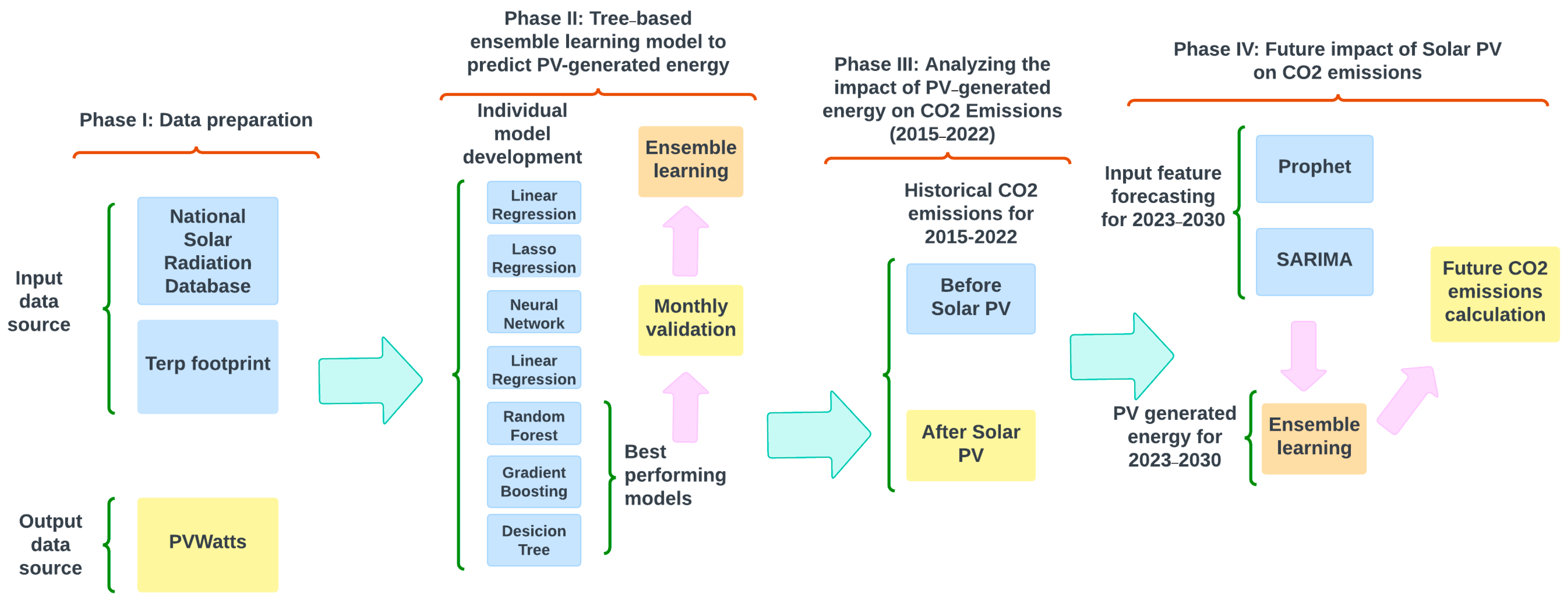
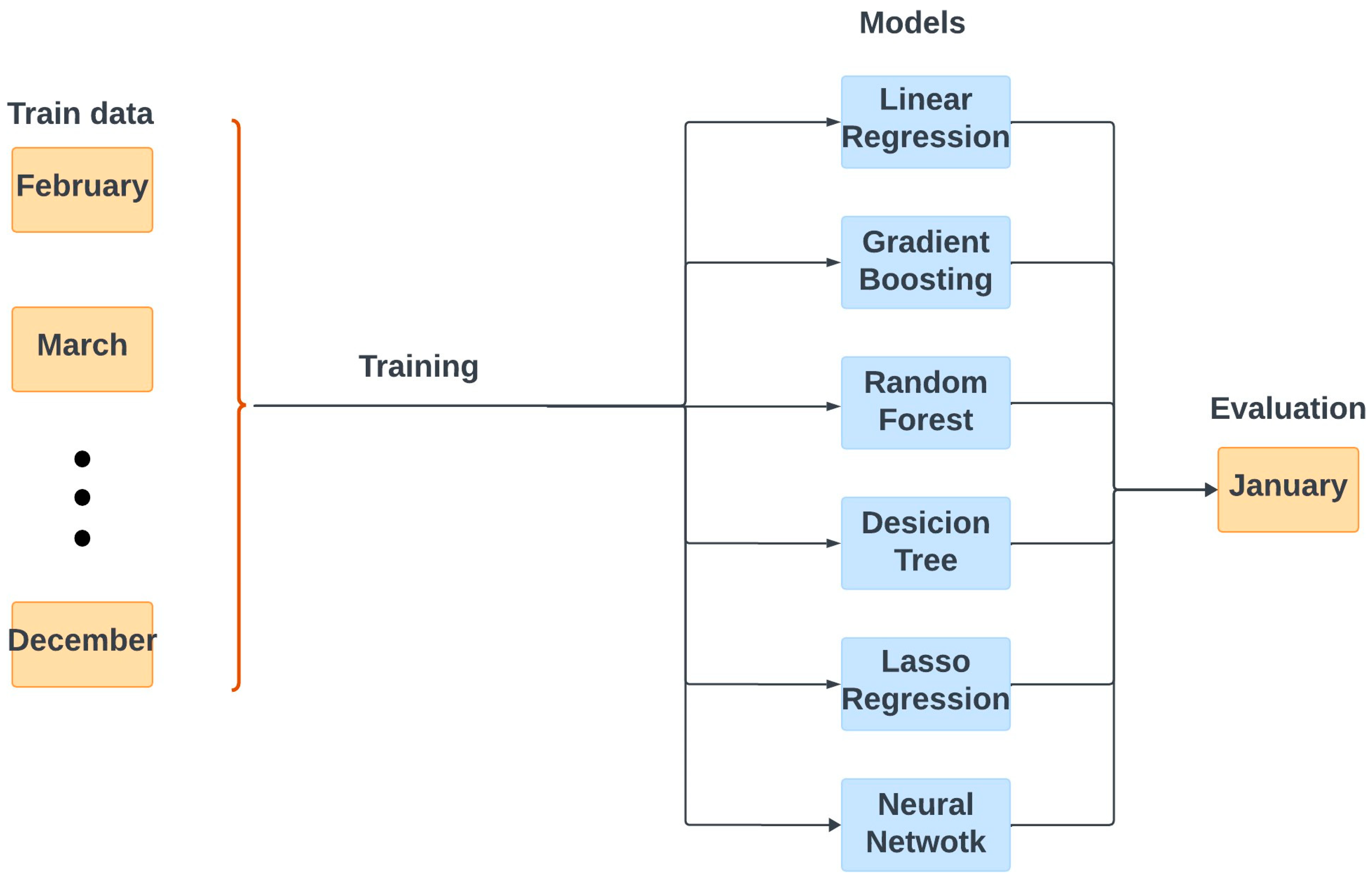
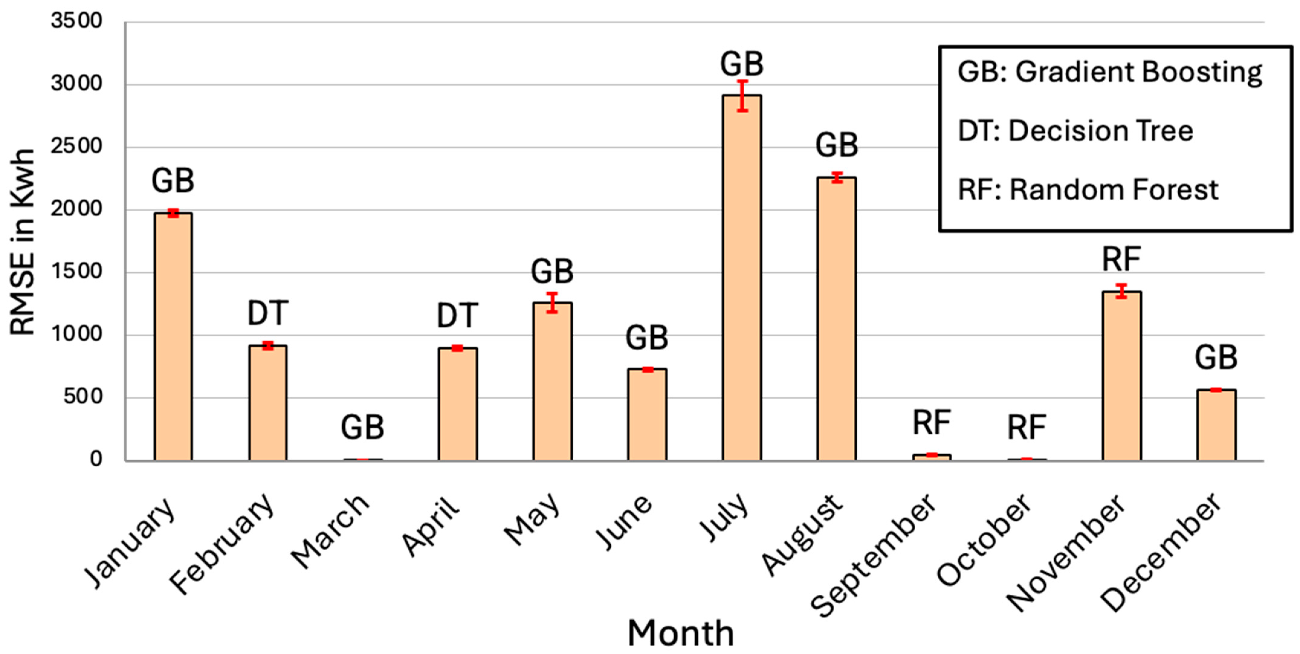
In this phase, various models were first implemented and tested individually. These included linear regression, lasso regression, neural networks, gradient boosting, decision trees, and random forest models. After evaluating the performance of each model across different months using the database of 153 buildings, the best-performing models were identified in order to develop a tree-based ensemble learning model and to optimize the performance by leveraging the strengths of each individual model.

3.2.1. Individual Model Development

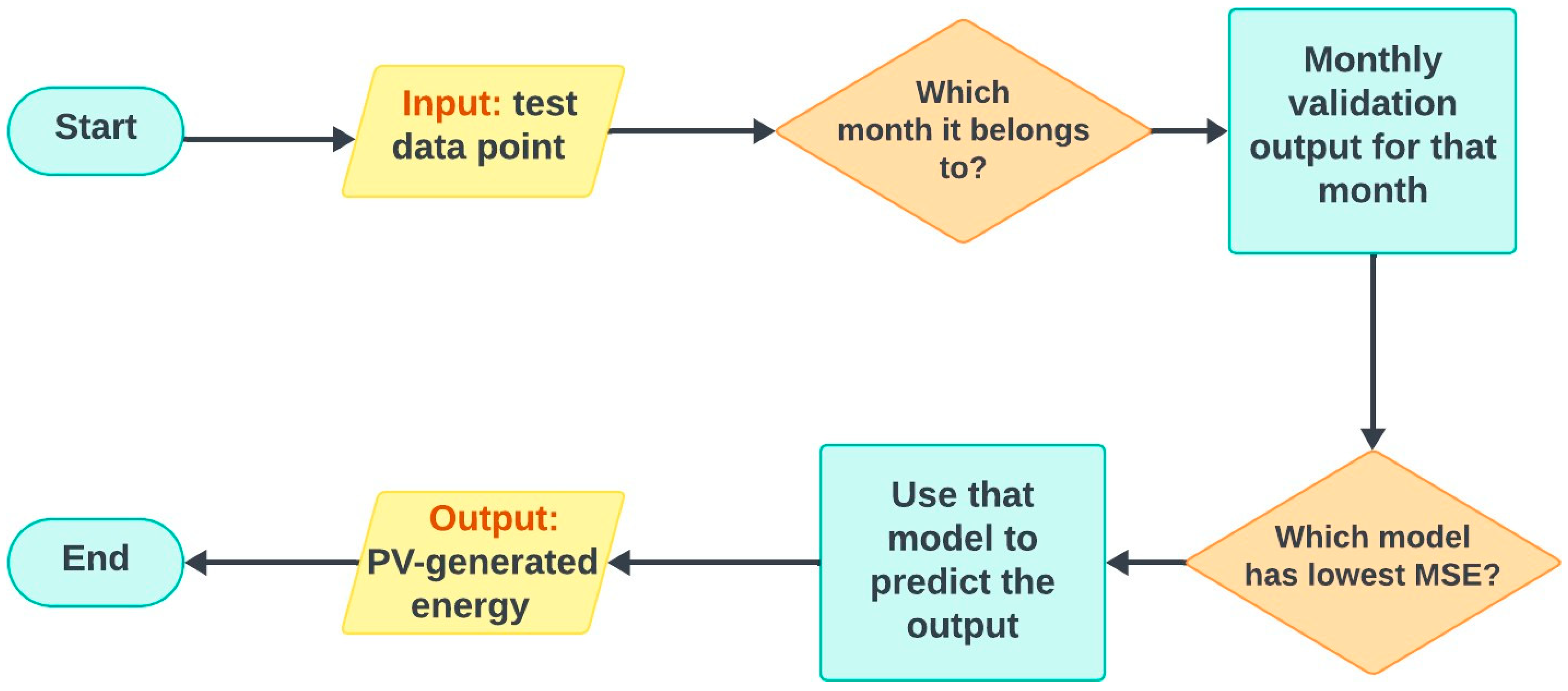
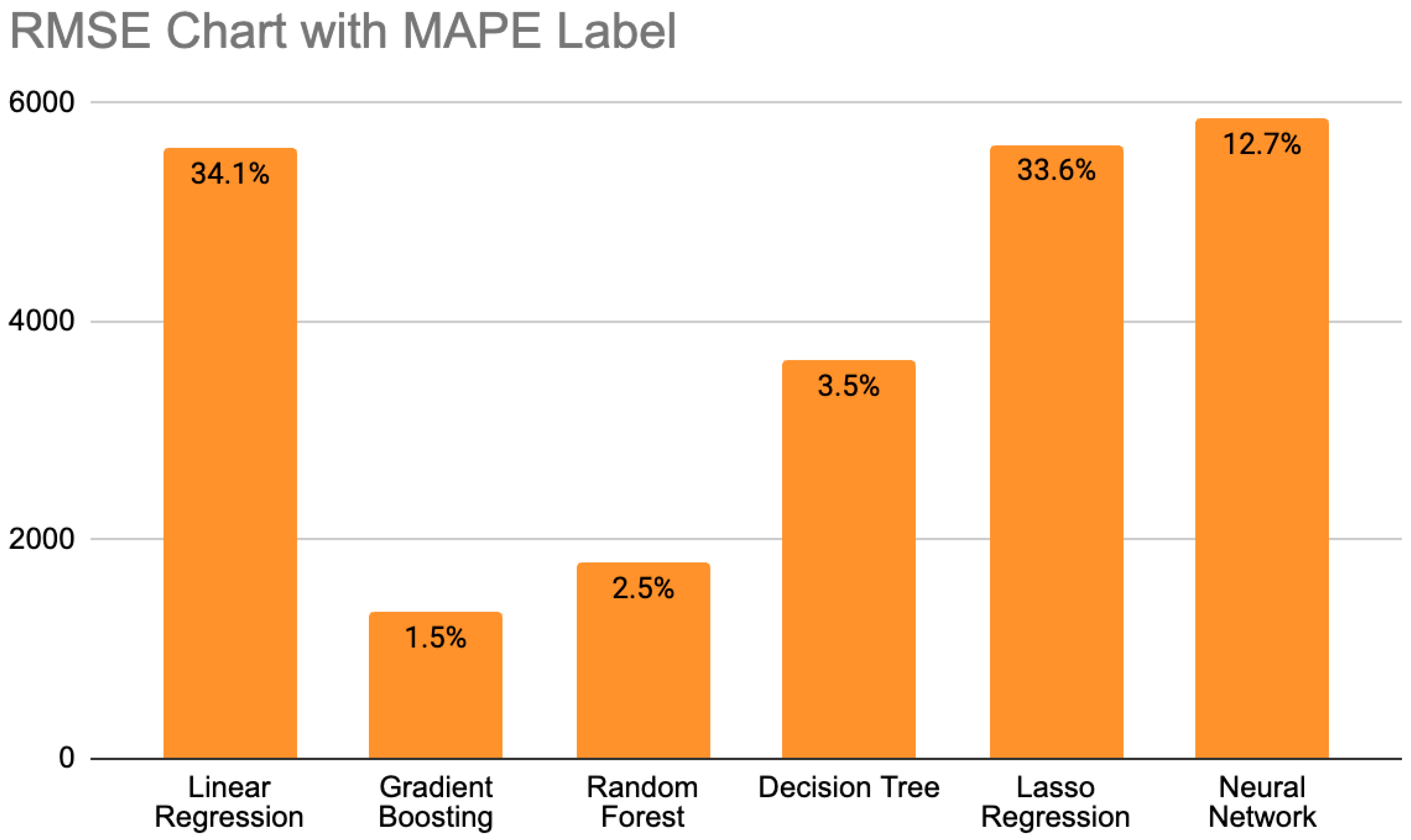
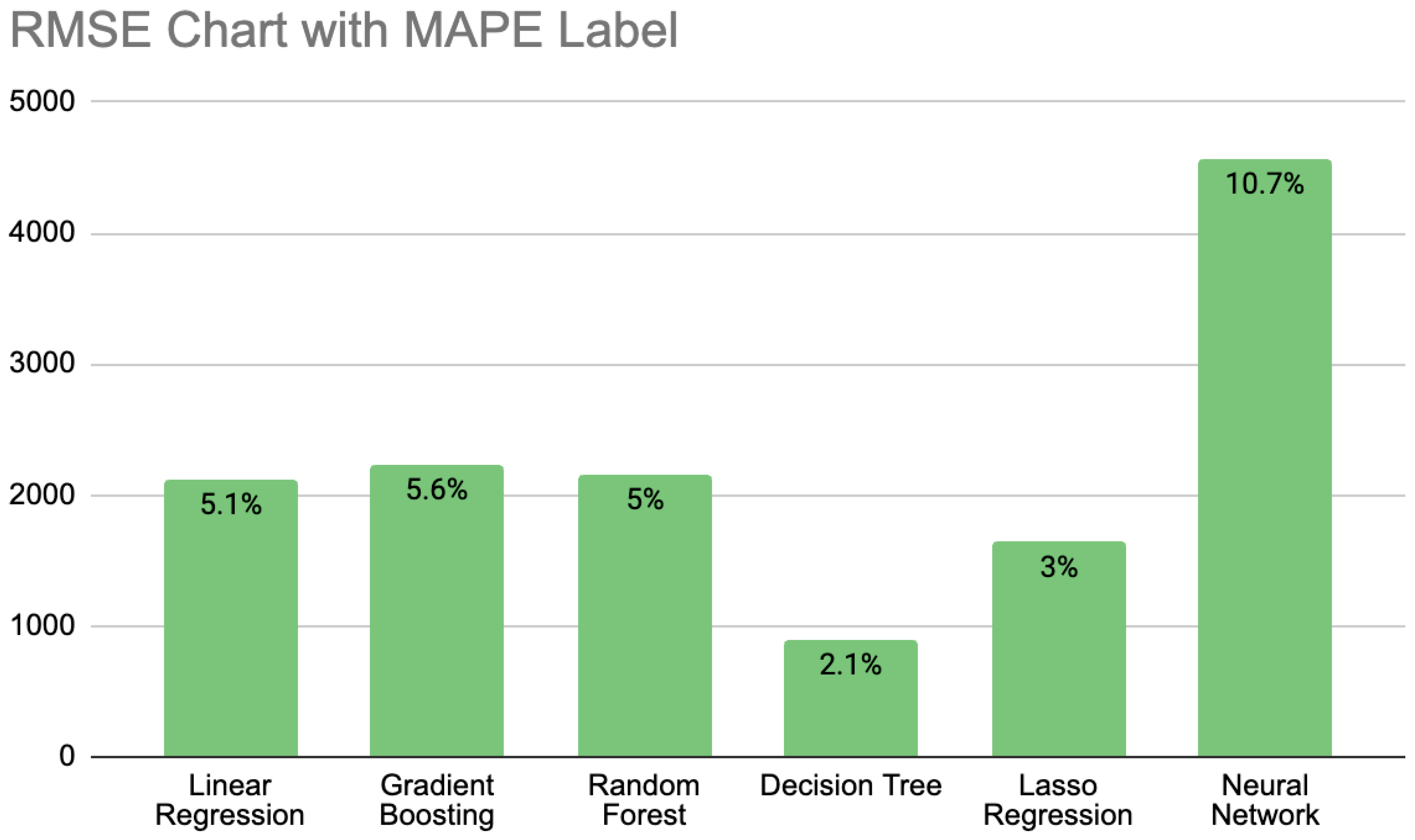
The first step of Phase II focused on implementing and evaluating various models, including linear regression, lasso regression, gradient boosting, random forest, decision tree, and neural networks, using the dataset prepared in Phase I. For each of the models, the best combination of features was studied to determine the optimal set. After training each individual model, including those listed above, the performance of each model was measured using root mean squared error (RMSE) and mean absolute percentage error (MAPE), shown in Equation (1) and Equation (2), respectively, which calculate the distance between the actual and predicted values.

$$\mathrm{R}\mathrm{M}\mathrm{S}\mathrm{E}=\sqrt{{\displaystyle \frac{1}{n}}{\sum }_{i=1}^n{(y_i-\widehat{y_i})}^2},$$

(1)

$$\mathrm{M}\mathrm{A}\mathrm{P}\mathrm{E}={\displaystyle \frac{1}{n}}{\sum }_{i=1}^n\left|{\displaystyle \frac{y_{i }-\widehat{y_i}}{y_i}}\right|\times 100$$

(2)

where $y_i$ represents the actual value, $\widehat{y_i}$ represents the predicted value, and n is the number of observations.

• Linear Regression:

Linear regression is a statistical technique used to model the relationship between a dependent variable Y and one or more independent variables X. The primary objective of linear regression is to predict the value of Y based on the given values of X by fitting a “best line” through the data points. This technique assumes that the relationship between the variables is linear, meaning that changes in the independent variable X are associated with linearly proportional changes in the dependent variable Y.

The linear relationship can be expressed mathematically, as shown in Equation (3):

$$Y\left(X\right)={\beta }_0+{\beta }_{1}X$$

(3)

where ${\beta }_0$ is the y-intercept and ${\beta }_1$ is the slope of the regression line. These coefficients are estimated using methods such as the least squares estimator (LSE), which minimizes the sum of squared differences between observed and predicted values of Y [29].

• Lasso Regression:

Lasso regression, or “Least Absolute Shrinkage and Selection Operator”, improves ordinary least squares (OLS) by adding a penalty based on the absolute values of coefficients. This method addresses overfitting and enhances interpretability, particularly with many predictors. By shrinking some coefficients to zero, Lasso effectively performs variable selection while minimizing the residual sum of squares within a constraint. This results in a simpler and more interpretable model.

The mathematical formulation of lasso regression can be expressed as follows:

$${\widehat{\beta }}^{Lasso}=arg {min}_{\beta }\left\{{\sum }_{i=1}^n{\left(y_i-{\beta }_0-{\sum }_{j=1}^p{\beta }_j{x}_{ij}\right)}^2\right\} \mathrm{s}\mathrm{u}\mathrm{b}\mathrm{j}\mathrm{e}\mathrm{c}\mathrm{t} \mathrm{t}\mathrm{o} {\sum }_{j=1}^p\left|{\beta }_j\right|\le t,$$

(4)

where t is a tuning parameter that controls the strength of the penalty. This constraint allows lasso regression to shrink less important coefficients to exactly zero, which simplifies the model by reducing the number of predictors. This approach balances bias and variance and leads to models with better predictive performance and easier interpretation than those produced by OLS, particularly when high-dimensional data are involved [30].

• Gradient Boosting

Gradient boosting is a powerful machine-learning technique that builds a predictive model by iteratively fitting weaker models to the residuals of previous iterations. The core idea is to minimize a loss function, L(y, F(x)), where F(x) is the model prediction and y is the true output. The process begins with an initial model, and in each iteration, the algorithm adds a new model that best reduces the loss function. This is achieved by fitting the new model to the negative gradient of the loss function with respect to the current model’s predictions. This approach can be formalized by solving the optimization problem $F^{\ast }={argmin}_F{E}_{y,x}\left[L\right(y, F\left(x\right)\left)\right]$, where the goal is to find the function F(x) that minimizes the expected loss.

In practice, gradient boosting involves constructing a model as a weighted linear combination of base learners, typically decision trees. The base learners are weak models that perform slightly better than random guessing. As described by the equation

$$F(x;\{{\beta }_m, a_m\})={\displaystyle \sum _{m=1}^M}{\beta }_{m}h(x;a_m)$$

(5)

where $h(x;a_m)$ represents the base learners, and each subsequent model in the sequence aims to correct the errors made by the previous ones. The algorithm determines the optimal parameters for these base learners using a steepest-descent approach. The gradient of the loss function guides the addition of new models. This iterative process continues until the model sufficiently reduces the loss function, leading to a strong predictive model [31].

• Random Forest

Random forests are an ensemble learning method that builds multiple decision trees during training and outputs the most common class (for classification) or average prediction (for regression). This method introduces randomness by randomly sampling training data (bagging) and selecting a subset of features for each tree split. This approach reduces model variance and helps prevent overfitting, particularly with noisy datasets. Each tree is trained independently, and the final prediction is an average of all trees’ predictions.

The generalization error of a random forest depends on the strength of the individual trees and the correlation between them. The margin function, which measures the extent to which the average number of votes for the correct class exceeds the votes for any other class, is a critical component in understanding the accuracy of the model. This can be mathematically expressed as

$$mr(X,Y)=P_{\Theta }\left(h\right(X,\Theta )=Y)-{min}_{j\ne Y}{P}_{\Theta }\left(h\right(X,\Theta )=j)$$

(6)

where ℎ(X, Θ) is the prediction of the tree classifier for a given input X, and Θ represents the random vector that governs the growth of each tree. A key insight provided by the analysis is that the generalization error decreases as the correlation between individual trees’ predictions decreases while maintaining a high strength for the individual trees [32].

• Decision Tree

Decision trees are a widely used machine learning algorithm that recursively partitions a dataset into subsets based on the value of input features, ultimately aiming to improve the prediction accuracy of the target variable. The basic idea behind decision tree construction is to select the feature that best splits the data into subsets, where one class dominates. This selection is based on the concept of information gain, which measures how well a feature separates the classes. The information gain, gain(A) from using feature A is calculated as the difference between the original entropy (a measure of uncertainty) and the weighted entropy after the split:

$$gain(A)=I(p,n)-{\displaystyle \sum _{i=1}^v}{\displaystyle \frac{p_i+n_i}{p+n}} I(p_i,n_i)$$

(7)

where I(p, n) is the entropy of the entire dataset and $I(p_i,n_i)$ is the entropy of each subset created by the split on feature A. Entropy is also defined as

$$I(p,n)=-{\displaystyle \frac{p}{p+n}}lo{g}_2{\displaystyle \frac{p}{p+n}}-{\displaystyle \frac{n}{p+n}}lo{g}_2{\displaystyle \frac{n}{p+n}}$$

(8)

where ${\displaystyle \frac{p}{p+n}}$ is the probability of an arbitrary object belonging to class P and ${\displaystyle \frac{n}{p+n}}$ refers to the probability of the same object belonging to class N.

The algorithm recursively splits data into subsets until they are “pure” (all members belong to a single class) or no further splits are meaningful. The ID3 algorithm prioritizes features with the highest information gain at each step, creating a tree structure where internal nodes represent features and branches represent feature values, with leaves indicating classification outcomes. While effective and interpretable, this method can be sensitive to noise and may lead to overly complex trees that overfit the data. Pruning strategies are used to remove less important branches, improving the model’s generalization to new data [33].

• Neural Network

Neural networks are computational systems inspired by the mammalian brain, designed to process data through layers of interconnected nodes, or “neurons.” These neurons receive inputs, process them via weighted connections, and use activation functions to produce outputs. The weights adjust during learning to minimize error. Neural networks excel in tasks like image recognition, machine translation, and pattern detection, making them powerful tools in machine learning and artificial intelligence [34].

In the proposed neural network model, as shown in Figure 3, two hidden layers with sizes of 64 and 32 neurons, respectively, are employed. The optimizer chosen for training the network is Adam, which stands for adaptive moment estimation. Adam combines the advantages of two other extensions of stochastic gradient descent: the ability to handle sparse gradients on noisy problems. The Adam optimizer updates the learning rate using the following formulas:

$$m_t={\beta }_1{m}_{t-1}+(1-{\beta }_1)g_t$$

$$v_t={\beta }_2{v}_{t-1}+(1-{\beta }_2)g_t^2$$

$$\widehat{m_t}={\displaystyle \frac{m_t}{1-{\beta }_1^t}}$$

$$\widehat{v_t}={\displaystyle \frac{v_t}{1-{\beta }_2^t}}$$

$${\theta }_t={\theta }_{t-1}-{\displaystyle \frac{\eta }{\sqrt{\widehat{v_t}+ϵ}}}\widehat{m_t}$$

(9)

where $g_t$ is the gradient of the objective function at time step t, $m_t$ and $v_t$ are the first and second moment estimates, ${\beta }_1$ and ${\beta }_2$ are the exponential decay rates for the moment estimates, $\widehat{m_t}$ and $\widehat{v_t}$ are bias-corrected moment estimates, η is the learning rate, and ϵ is a small constant to prevent division by zero [35].

The activation function used in the hidden layers is the rectified linear unit (ReLU). ReLU is a widely used activation function in deep neural networks, known for its simplicity and efficiency. It works by outputting the input directly if it is positive and zero otherwise, making it a non-linear function. This function is mathematically defined as

$$f\left(x\right)=max(x, 0)$$

(10)

where x is the input. ReLU’s main advantage is that it introduces non-linearity without saturating the gradients, as is often the case with sigmoid or tanh functions. This helps avoid issues like the vanishing gradient problem during training. In practice, ReLU is applied to the output of neurons in hidden layers, allowing the network to model complex patterns. Its effectiveness has been demonstrated across various deep-learning tasks, such as image classification, natural language processing, and speech recognition [36].

Parameter tuning was performed to optimize the model, including the selection of epochs, batch size, and other hyperparameters. Various configurations for the number of layers were also tested, with the best-performing architecture identified as a 2-layer model. Despite these efforts, the model consistently exhibited overfitting and did not demonstrate satisfactory performance, regardless of the parameter settings.

3.2.2. Monthly Validation

A monthly validation approach was adopted on the database of 153 buildings to thoroughly evaluate the performance of each model. For each month to be validated, the data corresponding to that month were excluded, and each model was trained on the remaining data. During the validation phase, the models were tested on the data for the specific month that was held out. For instance, according to Figure 4, to validate the models for January, the data for January were excluded from the training dataset. Each model was then trained on the data from the other 11 months, and its performance was evaluated on the January data during the validation phase. This process was repeated for each month individually to assess the model’s performance across different seasonal conditions and further finetune the hyperparameters for each model.

The validation process in this study followed a monthly validation approach, with k = 12 to reflect each month of the year in the same time span as the training data. The goal was to observe and assess the model’s performance on a monthly basis, enabling the evaluation of how it performs over time. This approach was specifically designed to capture the temporal dynamics of the data, providing insights into the model’s month-to-month performance. The methodology emphasizes performance stability across months rather than generalization across multiple validation folds.

The monthly validation approach (k = 12) was adopted to account for significant variability in weather conditions across months, which can influence model performance. Seasonal changes in weather patterns were hypothesized to impact prediction accuracy. Evaluating model performance on a monthly basis was deemed necessary to capture these fluctuations and gain insights into the model’s behavior over different time periods. This approach was selected to address temporal variability rather than relying on a fixed global validation framework.

3.2.3. Ensemble Learning

Ensemble learning is a powerful machine learning paradigm that combines multiple models to produce a single, superior predictive model. The idea is to aggregate the strengths of different models while mitigating their individual weaknesses. By combining the predictions of several models, ensemble methods often achieve better performance than any single model alone. This is particularly important in scenarios where the data or the target variable exhibits variability, as it allows the model to adapt and select the best approach for different subsets of the data [37].

Following monthly validation, it was observed that the performance of each model varied across different months. To leverage this variation and to obtain the best overall performance, an ensemble learning model was implemented. This ensemble model selects the best-performing model for each data point based on the month it belongs to. Since the best-performing models were gradient boosting, decision trees, and random forests, this method constitutes a tree-based ensemble learning approach.

As shown in Figure 5, for each test data point, the ensemble learning method identifies the corresponding month, searches the validation results for that month to find the best-performing model, and then uses that model to generate the PV energy output.

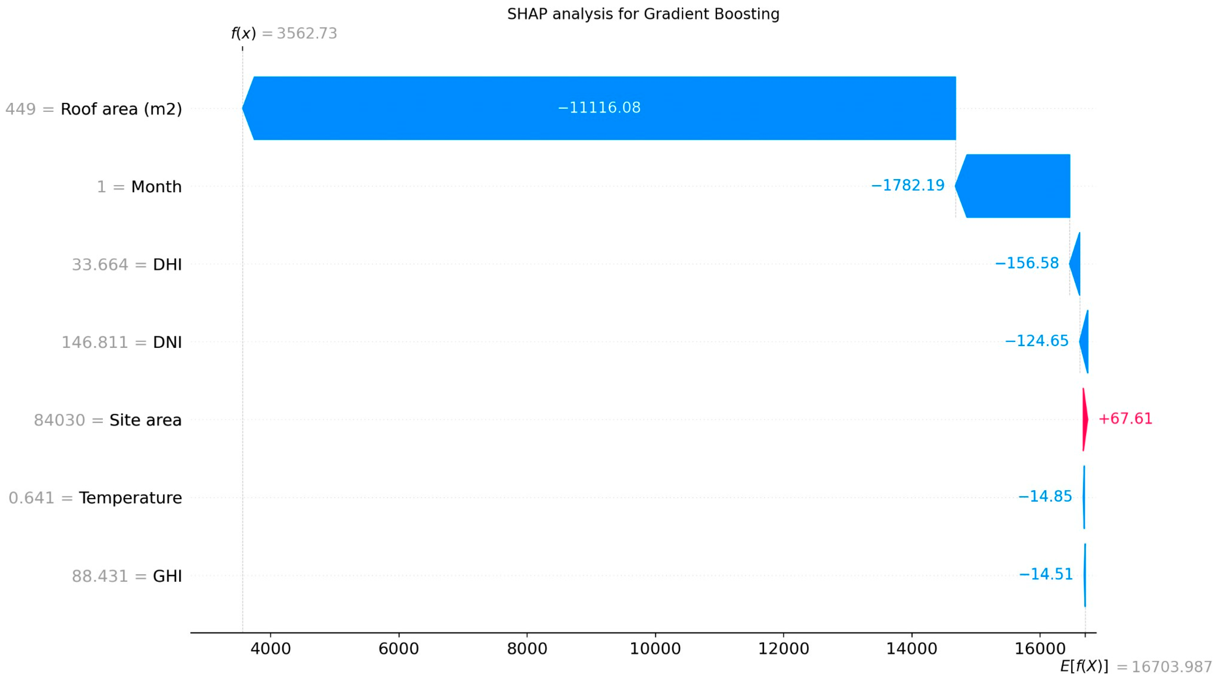
3.2.4. SHAP Analysis

SHAP (SHapley Additive exPlanations) is a method rooted in cooperative game theory that provides a unified approach to interpreting the predictions of machine learning models, particularly tree-based models. It calculates the contribution of each feature to the prediction by considering all possible feature combinations, ensuring that the explanations are both consistent and locally accurate. SHAP values uniquely satisfy properties of local accuracy, consistency, and missingness, making them ideal for understanding complex model behavior at both the local and global levels. This approach allows for detailed insights into how individual features interact to influence model predictions, offering a robust tool for model interpretability [38]. SHAP enhances the decision-making processes, leading to more informed and reliable interpretability.

To improve model interpretability, SHAP analysis was performed individually for each tree-based model utilized in the ensemble learning approach: gradient boosting, decision tree, and random forest. Figure 6 presents an example of SHAP results for the gradient boosting model and illustrates the contribution of each feature to the final prediction for a specific sample in the dataset.

For this purpose, we can take the mean SHAP values for each feature among all three tree-based models, as shown in

Table 1. Average SHAP values among different models.

	Gradient Boosting	Random Forest	Decision Tree
Roof area	18,129	18,219.34	18,294.4
Site area	275.26	156.8	203.72
Month	1787.96	1861.24	2153.26
DHI	275.56	109.29	138.93
DNI	131.28	66.4	127.43
GHI	47.62	88.46	274.52
Temperature	964.75	644.52	637.27

. The feature stability analysis across gradient boosting, random forest, and decision tree models reveals a high degree of consistency in SHAP values for most features. For instance, the SHAP values for the roof area (m²) remain tightly clustered around 18,000 across all three models, indicating strong agreement regarding its contribution. Similarly, features like the month show stable SHAP values, ranging from 1787 to 2153, demonstrating consistent importance across models. While some features, such as DHI and DNI, exhibit slight variability in SHAP values, their contributions are relatively stable.

The statistical significance analysis of feature rankings, as shown in

Table 2. SHAP p-values among different models.

	Gradient Boosting	Random Forest	Decision Tree
Roof area	0.000029	0.000002	0.072855
Site area	0.10322	0.155975	0.135876
Month	0.323399	0.114074	0.235859
DHI	0.517955	0.266058	0.337838
DNI	0.562686	0.642743	0.767929
GHI	0.579044	0.886380	0.154213
Temperature	0.873321	0.247264	0.247264

, reveals notable variations across the decision tree, random forest, and gradient-boosting models. For all three models, the roof area (m²) consistently emerges as the most significant predictor, with a p-value of 0.000002 in the random forest model and 0.000029 in gradient boosting, indicating strong statistical significance. In contrast, the decision tree model shows a relatively higher p-value of 0.072855 for this feature, suggesting marginal significance. Other features, such as the month and site area, demonstrate borderline significance in the random forest and gradient boosting models, but their p-values remain above the conventional threshold of 0.05, particularly in the decision tree model. Features like Temperature, GHI, DNI, and DHI consistently exhibit high p-values across all models, indicating they may not significantly contribute to the predictions. These results suggest that the random forest and gradient boosting models provide a more robust identification of key features with greater statistical confidence, while the decision tree’s rankings may be less stable or influenced by overfitting. This underscores the importance of considering multiple models to achieve a more reliable assessment of feature importance.

Several methods can be used to determine the feature importance threshold, with one practical approach being the setting of the threshold to the mean absolute value of SHAP values across all features. Using this threshold, the roof area is identified as the most significant feature, with an above-average SHAP value. This highlights the critical role of the roof area in the model’s predictions, a finding that is consistent across all three tree-based models employed in the analysis.

The addition of p-values provides insights into the statistical significance of the features in the proposed models, aiding in distinguishing between those with meaningful contributions and those that may not strongly relate to the model’s predictions. The standard threshold of 0.05 is used to assess statistical significance.

• A p-value below 0.05 indicates a strong relationship between the feature and the model’s predictions, suggesting that the feature’s importance is consistent and unlikely due to random chance. For instance, the roof area (m²) consistently demonstrates very low p-values (0.000002 in random forest and 0.000029 in gradient boosting), emphasizing its statistical significance across both models. This result confirms that the roof area is a key feature in all models.
• Conversely, a p-value above 0.05 suggests that the feature may not strongly relate to the model’s predictions. For example, the temperature, GHI, DHI, and DNI exhibit high p-values across all models, with values exceeding 0.05. The relatively low importance of features like GHI, DNI, and DHI can be attributed to the small geographic area of the University of Maryland, where weather and solar radiation conditions remain relatively uniform across the campus. Consequently, these features do not emerge as critical predictors due to their limited variability and impact on model performance.
• Features such as the site area and month show borderline significance in some models but have p-values above 0.05, suggesting that their contributions may vary across different models.

p-values thus provide a statistical foundation for evaluating the reliability of feature importance rankings. Features with low p-values, such as the roof area, are strongly supported as key contributors, while features with higher p-values indicate weaker or more variable effects. This highlights the value of using multiple models for feature selection, as models like random forest and gradient boosting consistently identify important features, whereas models like decision trees.

3.3. Phase III: Analyzing the Impact of PV-Generated Energy on CO₂ Emissions (2015–2022)

In this phase, the aim was to analyze the effect of PV-generated energy on reducing CO₂ emissions for the years 2015–2022 before exploring the effect for future years. The process involved predicting the PV-generated energy values for the years 2015–2022 based on the model developed in Phase II on a monthly basis. Since the final analysis was conducted on a yearly basis, a data preprocessing pipeline was implemented to convert the monthly data to yearly data. With the PV-generated values and emission factors in hand, the CO₂ emissions reduction achieved by solar PV implementation was calculated.

Without Solar PV implementation, the CO₂ emission is calculated as the following [39]:

$${{(CO}_2)}_{Before PV}=\mathsf{\Sigma }{ E}_i\times c_i,$$

(11)

where ${ E}_i$ refers to the energy consumption for each utility (gas, oil, electricity, etc.), and $c_i$ is the CO₂ emission factor for that specific utility.

While simulating the AC energy generated using rooftop Solar PV on PVWatts, system losses were considered and assumed to be ~14%. Furthermore, assuming the tilt and azimuth angles are 30° and 180°, respectively, the annual AC energy generated by rooftop Solar PV is calculated for every facility. For this study, a fixed (roof-mount Solar PV array) is assumed to be installed on the roof of every building. The Solar PV array is ~19% efficient and has the following parameters—DC to AC Size Ratio of 1.2, Ground Coverage Ratio of 0.4, and an Inverter Efficiency of 96%. These losses are factored into the final generation (E_pv). After solar PV implementation, since PV-generated energy helps reduce electricity consumption, it has to be subtracted from the original energy consumption. Also, the emissions caused by the solar PV installation were taken into account (0.0139 tons/GJ) [0.01465 tons per MMBTU] [40]:

$${{(CO}_2)}_{After PV}={{(CO}_2)}_{Before PV}-E_{pv}\times c_{elec}+0.01465\times E_{pv}$$

(12)

where ${{(CO}_2)}_{After PV}$ refers to the emissions after solar PV installation, $E_{pv}$ indicates the PV-generated energy, and $c_{elec}$ shows the electricity emission coefficient. The emission factors considered for this analysis are obtained from the EPA Power Profiler [41], which gives the annual coefficient of carbon dioxide equivalent (CO_2e) from electricity. An assumption of the study is that these coefficients remain the same over time to mimic the generation for a scenario where electricity generation from the grid does not become cleaner.

In some cases, the PV-generated energy might be greater than the original electricity consumption. In this case, the formula can be written as

$${{(CO}_2)}_{After PV}={{(CO}_2)}_{Before PV}-({min(E}_{pv},E_{elec})\times c_{elec})+0.01465\times E_{pv}$$

(13)

This study leverages the energy generated from rooftop Solar PV to develop a Tree-based ensemble learning model capable of predicting the energy generated from the arrays on individual buildings. Historical data from 2015 to 2022 have been used for this process to calculate the effect of generated PV energy on offsetting electricity consumption onsite. Photovoltaic (PV) systems experience degradation of about 0.5% to 1% per year. However, the impact on energy output by 2030 is minimal; for instance, a 0.5% annual degradation would reduce output by only 3.5% over 7 years. This reduction is often negligible in predictive models, especially Tree-Based Ensemble models, which focus on broader trends rather than fine details. Incorporating degradation effects requires extensive data on module age, maintenance, and specific degradation rates. This added complexity may risk overfitting the model without significantly improving predictive accuracy. For these reasons, a time-degradation model is ignored.

3.4. Phase IV: Predicting the Future Impact of Solar PV on CO₂ Emissions

In this phase, the primary objective was to predict and study the effect of solar PV installation on future CO₂ emissions. To achieve this, it was necessary to first forecast the CO₂ emissions without solar PV installation to establish a baseline for comparison. For predicting CO₂ emissions after solar PV implementation, the model developed in Phase II was utilized. This required implementing a meta-learning algorithm in which the model learns from forecasted solar radiation, wind speed, and temperature. By doing so, the future impact of solar PV on CO₂ emissions could be assessed, providing valuable insights for long-term planning and sustainability efforts.

3.4.1. CO₂ Emission Forecasting Until 2030

To project the impact of solar PV on future CO₂ emissions, CO₂ emissions without solar PV were forecasted until the year 2030 using support vector regression (SVR). Support vector regression is a regression technique rooted in the principles of support vector machines (SVM) introduced by Vapnik [42]. SVR seeks a function that approximates the target values within a tolerance of ϵ, ensuring minimal deviation while maintaining flatness in the solution space. The key feature of SVR is that it only considers errors greater than ϵ, allowing for the inclusion of a margin of tolerance in prediction. This approach ensures that the model is not overly sensitive to minor deviations from the target values, thus improving its generalization capabilities.

Mathematically, SVR is expressed as

$$f(x)={\displaystyle \sum _{i=1}^N}({\alpha }_i-{\alpha }_i^{\ast })K(x_i,x)+b$$

(14)

where x denotes the input vector, ${\alpha }_i$ and ${\alpha }_i^{\ast }$ represent Lagrange multipliers, $K(x_i,x)$ is the kernel function, and b is a bias term. The kernel function allows SVR to perform linear or non-linear regression depending on its choice of function (e.g., linear, polynomial).

The loss function employed by SVR is the ϵ-insensitive loss function, defined as

$$L(y,f(x\left)\right)=max(0,\left|y-f\left(x\right)\right|-ϵ)$$

(15)

This loss function ensures that any prediction within ϵ of the actual value incurs no penalty, while deviations exceeding ϵ are penalized proportionally to their magnitude. This approach strikes a balance between model accuracy and generalization by allowing the model to ignore minor errors [42].

3.4.2. Input Feature Forecasting

To predict future CO₂ emissions after solar PV implementation, it was necessary to forecast the input features, such as solar radiation and other related variables. Given that all input features exhibit a 12-month seasonality pattern, two different forecasting models were employed: Prophet and SARIMA. Prophet is a time series forecasting model developed by Facebook [43]. It is particularly effective when there is a strong seasonal effect and missing data. Prophet is capable of handling shifts in trends, making it a versatile tool for forecasting time series data with complex seasonal patterns. SARIMA (Seasonal Auto Regressive Integrated Moving Average) is an extension of the non-seasonal ARIMA model designed to capture seasonality in the data [44]. Both Prophet and SARIMA were implemented using default hyperparameters, with the period of 12 considered to account for monthly seasonality.

Table 3. Comparison of differences and strengths between SARIMA and Prophet.

SARIMA	Prophet
Time series forecasting method	Time series forecasting method
Extension of non-seasonal ARIMA to capture seasonality	Best when there is strong seasonal effect
Captures short-term and long-term dependencies	Robust with missing data and handles shifts in the trends

summarizes the key differences between these two methods and emphasizes their respective strengths.

3.4.3. Meta-Learning Algorithm

Meta-learning, often referred to as “learning to learn,” is a subfield of machine learning where algorithms are designed to learn how to optimize other learning algorithms. The primary goal of meta-learning is to improve the adaptability and performance of models by using knowledge gained from prior learning experiences [45]. Meta-learning models can quickly adapt to new tasks with minimal data. This makes them particularly useful in dynamic environments where conditions change rapidly.

In this study, the input features forecasting data were utilized to feed into the ensemble learning model to form a meta-learning algorithm. By leveraging the predicted values of solar radiation, wind speed, and temperature, the ensemble learning model was able to refine its predictions of PV-generated energy and CO₂ emissions. This meta-learning approach enabled the model to adapt to the seasonal patterns and trends in the input data, which enhanced the overall accuracy and robustness of future PV-generated energy predictions.

The final model was not computationally intensive and could be efficiently executed on a standard CPU, such as the M2, with 8–12 GB of RAM. It did not require significant memory or specialized hardware, such as GPUs, making the model feasible to run using basic computational resources.

4. Results and Discussion

This section presents an analysis of the model performances, validation processes, and comparative assessments against related works. It begins with the evaluation of individual models, where their accuracy in predicting PV-generated energy is assessed using metrics such as root mean squared error (RMSE) and mean absolute percentage error (MAPE). The section then explores the monthly validation results, emphasizing the consistent superiority of tree-based models across different months. Additionally, it explores input feature forecasting using SARIMA and Prophet and provides insights into their predictive capabilities for solar radiation data and how they are utilized to develop a meta-learning method. The section concludes with a benchmarking analysis that highlights the proposed method’s distinct advantages, including the use of ensemble and meta-learning, interpretability, and a unique focus on long-term forecasting and emissions study.

4.1. Phase II Results

Phase I begins with the development of individual models, focusing on evaluating various approaches. As illustrated in Figure 7, the results from this phase demonstrate that tree-based models—namely gradient boosting, decision tree, and random forest—consistently outperformed the other methods. These models achieved mean absolute percentage error (MAPE) values below 5% and root mean square error (RMSE) under 4000, highlighting their robustness and superior accuracy in predicting PV-generated energy.

The model selection was grounded in a comprehensive comparison where these algorithms consistently outperformed deep learning approaches, which, despite multiple optimization rounds, exhibited overfitting tendencies and showed limitations in generalizing the dataset well. While neural networks were implemented and optimized, their predictive accuracy did not surpass that of tree-based models for our task requirements.

Additionally, tree-based models were more aligned with the project’s need for interpretability and computational efficiency, especially critical given the scale and complexity of the dataset. Ensemble techniques, such as those provided by random forest and gradient boosting, enabled robust prediction with lower variance, an advantage deep learning approaches could not replicate within the operational constraints.

The potential overfitting of the deep learning model was examined by calculating both bias and variance. A low bias combined with a high variance is indicative of overfitting, while the opposite suggests underfitting.

Table 4. Bias-Variance Tradeoff Across Varying Epochs.

Epoch	Bias (kWh)	Variance (kWh)
500	339.48	4,581,649.5
1000	−294.5	2,838,604.5
2000	−141.9	2,529,968.0
4000	−329.15	6,171,358.5
5000	−121	6,925,971.5

presents the bias and variance values for the model as the number of epochs is varied (500, 1000, …, 5000). As shown in Table 4, the variance values are consistently much higher than the bias values across all epochs, confirming the presence of overfitting in the model. For instance, at 500 epochs, the bias is 339.48 kWh, while the variance is significantly higher at 4,581,649.5 kWh. This trend persists as the number of epochs increases, further reinforcing the observation of overfitting.

These results provide quantitative evidence of overfitting, which has been addressed through strategies such as early stopping, regularization, and reduced model complexity. This analysis strengthens the validity of the findings and the steps taken to mitigate overfitting in the study.

A monthly validation process was conducted to assess the models’ performance over time. As seen in Figure 8, significant variations in performance were observed across different months. Despite this, tree-based models, particularly gradient boosting, consistently outperformed other models throughout all 12 months. This establishes the tree-based models as potential candidates for ensemble model development.

Building on these findings, an ensemble learning technique was developed to combine the strengths of individual models. The performance of the tree-based ensemble model, as developed in Phase I, resulted in an RMSE of 1429.64 kWh and a MAPE of 1.7%. Although this ensemble model showed slightly lower performance than the best individual model, the principles behind ensemble learning suggest that it will offer greater robustness when applied to larger datasets.

As illustrated in Figure 9, the decision tree model demonstrated the best performance for April, achieving a MAPE of 2.1%. Similarly, each month had its own best-performing model, and these models were incorporated into the ensemble learning framework.

The p-values derived from paired t-tests between the RMSE values of different tree-based models across months are shown in

Table 5. p-values from paired tests between RMSE values of different tree-based models.

Pair	p-Value
Gradient Boosting vs. Decision Tree	0.2475
Gradient Boosting vs. Random Forest	0.1564
Decision Tree vs. Random Forest	0.3628

. These values suggest that the models perform similarly across months in terms of RMSE. This finding supports the idea that combining these models could be beneficial, as it would allow the meta-learning approach to draw on the strengths of each model, potentially improving forecasting accuracy by integrating their complementary capabilities.

The mean absolute percentage error (MAPE) of 1.7% for the ensemble learning model indicates that, on average, the predicted values deviate from the true values by ±1.7%. This margin of error reflects the typical prediction variability and provides a clear measure of the model’s accuracy. The uncertainty level for the MAPE value itself is ±0.1%, based on the calculation method, which may involve rounding. Therefore, the predicted CO₂ reduction values could be within ±1.7% of the true values, demonstrating the model’s high degree of predictive reliability.

To further validate the results, the proposed model’s predictions were compared with estimates generated by the system advisor model (SAM, 2023.12. 17 Revision 2, SSC 292), a software by the National Renewable Energy Laboratory (NREL) that provides monthly PV-generated energy estimates based on inputs such as location, system size, and year. Figure 10 presents the PV-generated energy calculated by both SAM and the machine learning model for the years 2015–2022, covering two different buildings on the UMD campus. The comparison revealed an average percentage difference of approximately 3.42% between this model’s predictions and SAM’s outputs. A certain level of discrepancy between machine learning predictions and actual outcomes is expected due to the inherent variability in real-world data and model assumptions. These differences can be minimized, but they cannot be entirely eliminated. Weather data from 2018 likely had unique patterns or anomalies compared to the training data (TMY2020), which could lead to prediction discrepancies. The trends from TMY2020 might not fully encapsulate the specific characteristics of 2018, demonstrating a limitation in the generalizability of the model’s assumptions to certain years.

4.2. Phase III Results

Figure 11 and Figure 12 illustrate the comparison of historical CO₂ emissions before and after solar PV implementation, as calculated using Equations (11) and (12), for two different buildings within the UMD campus. The magnitude of the difference between these values depends on the primary energy source. Specifically, when electricity is the primary energy source, a significant reduction in CO₂ emissions is observed post-solar PV implementation. Conversely, when other energy sources predominate, the reduction in CO₂ emissions tends to be less substantial.

4.3. Phase IV Results

Phase IV begins with forecasting CO₂ emissions for future years without the implementation of solar PV, serving as a baseline for comparison with the scenario where solar PV is installed. The forecast using SVR, shown in Figure 13, demonstrated a 16% error rate, indicating a relatively high level of accuracy.

Moreover, this phase focuses on forecasting solar radiation and related input features for future years, which lays the groundwork for predicting CO₂ emission reductions associated with solar PV implementation. Figure 14 presents the results of applying both Prophet and SARIMA forecasting methods to solar radiation data. Figure 14 includes actual values up to 2022, followed by forecasted values for global horizontal irradiance (GHI). As observed, the SARIMA model exhibits a repetitive and cyclical pattern, while the Prophet model introduces more nuanced variations, resulting in forecasts that appear to align more closely with real-world trends.

Although the performance metrics of Prophet and SARIMA are quite close, as shown in

Table 6. Comparison between Prophet and SARIMA in terms of MAE, RMSE, and Pearson Correlation.

Forecasting Model	MAE (W/m2)	RMSE (W/m2)	Pearson Correlation
Prophet	40.59	61.89	0.811
SARIMA	38.75	58.54	0.808

, the trend predicted by Prophet appears more natural and less repetitive, with a slightly stronger correlation to historical data.

Building on this forecasting foundation, a meta-learning algorithm was developed to predict future PV-generated energy and, consequently, CO₂ emissions reductions due to solar PV adoption. Figure 15 illustrates a significant reduction in CO₂ emissions following the deployment of solar PV systems. While the SARIMA and Prophet models generated different forecasting results, their overall impact on emissions reduction was quite similar. This suggests that despite differences in predictive mechanisms and specific forecasts, both models offer a consistent and reliable assessment of emissions trends. Therefore, it can be concluded that these forecasting methods, though varied, provide a dependable basis for evaluating future emissions reduction with solar PV. The close-to-flat line towards the end occurs because, after reaching a certain level of accuracy, the profit and RMSE outputs become consistent. This leads to repetitive inputs for the meta-learning algorithm, ultimately producing a stable, flat output. The forecast horizon was set to 2030, as the available eight years of historical data support reliable predictions up to this point. Extending the horizon beyond 2030 showed a natural flattening of the model’s predictions, reflecting the challenges of forecasting further into the future with limited data coverage.

The meta-learning approach in this study builds on the same ensemble learning model whose performance was validated and quantified in Phase II. Meta-learning, in this context, involves learning from the outputs of other machine learning algorithms, specifically SARIMA and Prophet, which were also validated for their performance. This ensures that the meta-learning approach is based on well-validated models, providing a basis for more informed forecasting.

4.4. Benchmarking Against Related Work

Table 7. Comparison between the related work and proposed method.

	Tahir et al. [19]	Perera et al. [20]	Mitrentsis et al. [21]	Ray et al. [22]	This Work
Ensemble learning or Meta-learning	Ensemble learning	None	None	None	Ensemble learning and Meta-learning
Interpretability	✖	✖	✔	✖	✔
Future forecasting	✔	✔	✔	✔	✔
Long-term future forecasting	✖	✖	✖	✔	✔
Emissions study	✖	✖	✖	✖	✔

presents a comparative analysis of related work against the proposed method in terms of several key criteria: the use of ensemble learning or meta-learning, interpretability, future forecasting, long-term future forecasting, and emissions study. The works by Tahir et al. and the proposed method both utilize ensemble learning, with the proposed method additionally incorporating meta-learning. In contrast, other referenced works do not utilize ensemble or meta-learning. When considering interpretability, this work and Mitrentsis et al. method provide interpretable results, unlike the others. All referenced works, including the proposed method, address future forecasting, but only Ray et al. and the proposed method focus on long-term future forecasting. Finally, the proposed method is unique in integrating an emissions study with PV-generated energy predictions, setting it apart from other works. This dual-focus approach provides a holistic perspective, addressing both energy efficiency and environmental impact within a single framework. Additionally, the implementation of a monthly validation methodology ensures that the seasonal variations in solar energy generation are accurately captured, enhancing the robustness of the ensemble learning models.

5. Conclusions

This study aimed to predict and analyze the impact of solar PV implementation on CO₂ emissions using a comprehensive machine learning approach. The methodology involved multiple phases, including data preparation, model development, performance evaluation, and forecasting. The results demonstrated the effectiveness of tree-based models and ensemble learning in predicting PV-generated energy and their subsequent impact on CO₂ emissions. The accuracy of the predictions was validated using established tools such as SAM, confirming the reliability of the proposed models, which demonstrated an error rate of ~3.5%.

In Phase I, detailed data preparation ensured a robust dataset for model training. Phase II involved the development and evaluation of various models, with ensemble tree-based models showing superior performance with RMSE of 1429.64 kWh and MAPE of 1.7%. Phase III focused on analyzing historical CO₂ emissions reductions, while Phase IV projected future impacts of Solar PV installations. SHAP analysis was conducted to enhance the interpretability of the models, while the integration of Prophet and SARIMA models with over 0.8 correlation provided accurate forecasts of input features, contributing to the overall prediction accuracy.

This work offers a valuable tool for CO₂ and solar PV analysis, particularly in the context of campus data. To further enhance its applicability, future research could extend the analysis to diverse datasets from various geographical locations and building types. Additionally, while this study assumed 50% of the roof area for solar PV installation, exploring different percentages in future studies could yield further insights. The integration of advanced techniques, such as large language models (LLMs), could also be investigated to potentially boost prediction accuracy and model interpretability, offering new avenues for further enhancing the models’ performance.