The Levenberg–Marquardt Procedure for Modeling Accelerometers Used in the Energy Industry

Abstract

This paper presents an effective Levenberg–Marquardt procedure for modeling accelerometers used in the energy industry. The proposed procedure applies the results of accelerometer calibration methods commonly used in engineering practice using stationary or portable calibrators. These methods are extended here to more advanced solutions, which will constitute the basis for further research (both practical and theoretical) for improving the accuracy of accelerometers, which play an extremely important diagnostic function in the operation of machines, devices, and the wide range of components used in the energy industry. The research results presented in this article were obtained using MathCad 15 and MATLAB R2024a software.

1. Introduction

Accelerometers have very important functions in applications in the energy industry, especially in the field of monitoring and diagnostics of the operation of machines and devices [1,2]. They play an important role in the early detection of damage by monitoring the operation of bearings in generators, engines, turbines, and various types of pumps and compressors [3]. Such sensors play a particularly important role in wind power plants, where they are used to monitor rotor vibrations caused by damage, balancing errors, or the influence of atmospheric factors [4,5]. They are also very important components of hydroelectric power plants, as they detect vibrations of rotors or other moving elements [6]. Nuclear power plants are used for early detection of earthquakes or seismic effects, which negatively affect the operation of this type of power plant [7]. In addition, they are used to monitor transmission infrastructure to ensure the stability of high-voltage lines and supporting structures [8,9] and are indispensable diagnostic elements designed to detect leaks in oil or gas pipelines by monitoring changes in pressure or flow dynamics [10,11].

Due to the wide range of very important applications of accelerometers in the energy industry, systematic control systems are necessary, as their improper operation would disrupt the correct diagnostics and monitoring of the energy infrastructure [12]. Accelerometer control is carried out by means of calibration, which is carried out using specialized stationary calibrators or portable calibrators, which are becoming increasingly popular. This calibration is carried out by determining two basic characteristics as follows [13,14]:

–

Linearity, which represents the dependence of the response signal amplitude on the excitation signal at a constant excitation frequency;

–

Amplitude–frequency response, which represents the relationship between the output signal amplitude to the input signal amplitude ratio and the changes in frequency over the range covering the accelerometer’s operating frequency band.

However, in addition to the abovementioned calibration methods, which are traditionally applied in engineering practice, a very important role is also played by the elimination of the dynamic error during the operation of the accelerometer at the diagnostic station [15]. The dynamic error is then the result of stimulating the accelerometer with dynamically changing undetermined signals, i.e., signals that are not repeatable as a function of time [16,17,18]. The dynamic error is typically eliminated using deconvolution filters, which perform inverse transformations [19]. However, such a transformation is only possible when the parameters of the mathematical model of the accelerometer (usually a second-order differential equation) are determined by modeling. This can be performed by determining the amplitude–frequency response of the corresponding accelerometer, but there is a need to regulate the frequency over a range that exceeds the resonance state [20].

This paper presents a method of modeling accelerometers based on an iterative Levenberg–Marquardt procedure, which is used for regression of the amplitude–frequency response measurement points according to the least squares principle [21,22]. This procedure combines the Gauss–Newton and steepest descent methods and is, therefore, extremely effective for nonlinear regression tasks, such as determining the amplitude–frequency response. The solutions presented in this paper are based on the measurement points of this response and are obtained by using the same portable calibrator as applied in the classical calibration of accelerometers.

Section 2 introduces some theoretical background to accelerometer modeling using second-order differential equations, derives mathematical formulas related to the amplitude–frequency response, and presents a detailed discussion of applying the Levenberg–Marquardt procedure to accelerometer modeling. Section 3 gives the calibration and modeling results of two selected accelerometer types. An example of the use of the deconvolution algorithm to eliminate the dynamic error of an accelerometer is also presented.

The solutions presented here constitute a new approach to accuracy tests of accelerometers in energy applications and can be successfully used in engineering practice, as a supplement to commonly applied calibration methods based on this type of sensor, and in theoretical studies of the optimization of mathematical models of accelerometers, elimination of the dynamic error, and determination of the upper limit of the dynamic error, among others [20]. These solutions can significantly improve the diagnostic measurements performed by accelerometers in energy applications.

In addition to the solution presented in the paper, it is also possible to use the optimization procedure based on the Monte Carlo method [23]. This method is based on the pseudorandom number generator with a predetermined statistical distribution (uniform or Gaussian), and the input data for this method are intuitively defined parameters of the mathematical model of the accelerometer (the amplitude–frequency response). The main disadvantage of this method is the need to implement the pseudorandom number generator and the need to generate a significant number (over $2\times {10}^5$ trials) of Monte Carlo generations.

2. Materials and Methods

The mathematical model of the accelerometer is described by a second-order differential equation as follows:

$$\ddot{y}+2{\omega }_0\beta \dot{y}+{\omega }_0^{2}y=-S_{\mathrm{k}}{\omega }_0^2,$$

(1)

where $S_{\mathrm{k}} [\mathrm{V}/\mathrm{g}],$ ${\omega }_0 [\mathrm{r}\mathrm{a}\mathrm{d}/\mathrm{s}]$, and $\beta [-]$ denote the static amplification factor, pulsation of natural undamped vibrations, and damping factor, respectively, while $x$ and $y$ are the excitation amplitude in $\mathrm{g}$ and accelerometer response in V.

The Laplace transform of the above equation with zero initial conditions gives

$$Y\left(s\right)s^2+2{\omega }_0\beta Y\left(s\right)s+{\omega }_0^{2}Y\left(s\right)=-S_{\mathrm{k}}{\omega }_0^{2}X\left(s\right),$$

(2)

where $s=\mathrm{j}\omega$ denotes a Laplace operator and $\mathrm{j}=\sqrt{-1}$ is the imaginary number.

A simple transformation of Equation (2) gives the formula

$$K(s)=Y(s)/X(s)={\displaystyle \frac{-S_{\mathrm{k}}{\omega }_0^2}{s^2+2{\omega }_0\beta s+{\omega }_0^2}},$$

(3)

which represents the transfer function for the accelerometer [24].

When Equation (3) is considered as the accelerometer frequency response, we have

$$K(\mathrm{j}\omega )=A(\omega ){\mathrm{e}}^{\mathrm{j}\phi \left(\omega \right)},$$

(4)

where $A(\omega )$ and $\phi (\omega )$ represent the amplitude–frequency and phase–frequency responses of the accelerometer. The following equations represent these responses:

$$A(\omega )=\left|K(\mathrm{j}\omega )\right|={\displaystyle \frac{S_{\mathrm{k}}}{\sqrt{{\left(1-{\left(\frac{\omega }{{\omega }_0}\right)}^2\right)}^2+{\left(2\beta \left(\frac{\omega }{{\omega }_0}\right)\right)}^2}}}$$

(5)

and

$$\phi (\omega )=\mathrm{a}\mathrm{r}\mathrm{g}\left(K\left(\mathrm{j}\omega \right)\right)=-\mathrm{a}\mathrm{r}\mathrm{c}\mathrm{t}\mathrm{g}{\displaystyle \frac{2\beta \frac{\omega }{{\omega }_0}}{1-{\left(\frac{\omega }{{\omega }_0}\right)}^2}},$$

(6)

where $\omega =2\mathsf{\pi }f$ [rad/s] and $f$ [Hz] is the frequency [24].

In the following, we present graphical dependencies and mathematical relations that constitute the basis for modeling the accelerometer based on the amplitude–frequency response.

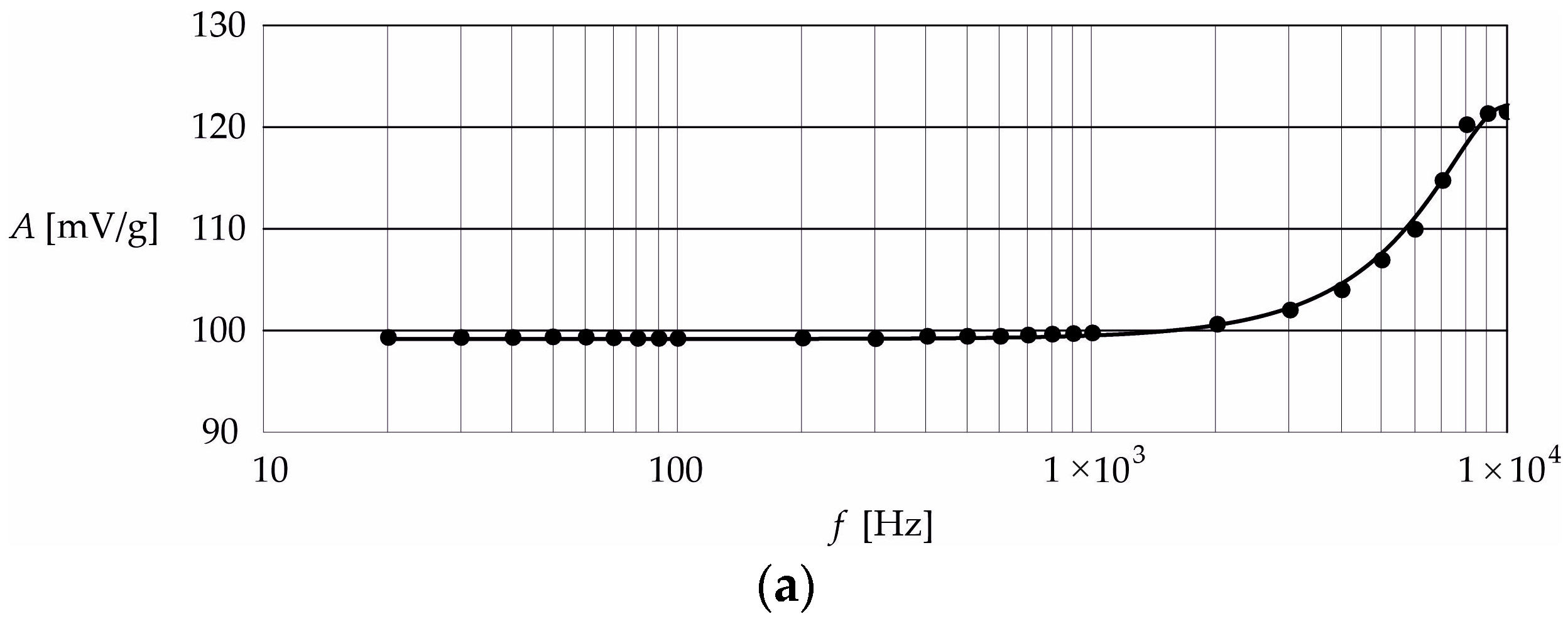
Figure 1 shows an exemplary amplitude–frequency response as a function of frequency, where $f_{\mathrm{r}}$ and ${\mathrm{p}}_{\mathrm{r}}$ denote the resonance frequency and resonance peak, respectively. These parameters are typical variables for accelerometer modeling based on the amplitude–frequency response.

The resonant frequency is obtained by equating the following derivative to zero:

$${\displaystyle \frac{\mathrm{d}}{\mathrm{d}f}}\left[A\left(f\right)\right]={\displaystyle \frac{-S_{\mathrm{k}}\left[\frac{2f}{\mathsf{\pi }{f_0}^2}\left({\left(\frac{f}{f_0}\right)}^2-1\right)+8{\beta }^2\frac{f}{{f_0}^2}\right]}{2 \sqrt[3]{{\left[{\left(\frac{f}{f_0}\right)}^2-1\right]}^2+4{\beta }^2{\left(\frac{f}{f_0}\right)}^2}}}=0.$$

(7)

Simplification of Equation (7) gives

$$f=f_{\mathrm{r}}=f_0 \sqrt{1-{2\beta }^2}.$$

(8)

The ordinate value corresponds to $f_{\mathrm{r}}$ and defines the resonance peak

$$A\left(f_{\mathrm{r}}\right)={\mathrm{p}}_{\mathrm{r}}={\displaystyle \frac{S_{\mathrm{k}}}{2\beta \sqrt{1-{\beta }^2}}}.$$

(9)

Solving Equation (9) gives

$$\beta ={\displaystyle \frac{ \sqrt{{\mathrm{p}}_{\mathrm{r}}-\sqrt{{{\mathrm{p}}_{\mathrm{r}}}^2-{S_{\mathrm{k}}}^2}}}{\sqrt{2{\mathrm{p}}_{\mathrm{r}}}}}.$$

(10)

Substituting Equation (10) into transformed Equation (8) gives

$$f_0={\displaystyle \frac{f_{\mathrm{r}}}{\sqrt{1-\frac{{\mathrm{p}}_{\mathrm{r}}-\sqrt{{{\mathrm{p}}_{\mathrm{r}}}^2-{S_{\mathrm{k}}}^2}}{{\mathrm{p}}_{\mathrm{r}}}}}}.$$

(11)

By substituting Equations (10) and (11) into Equation (5), as a function of the frequency $f$, we obtain

$$A(f)={\displaystyle \frac{S_{\mathrm{k}}}{\sqrt{{\left(1-{\left(\frac{f}{\frac{f_{\mathrm{r}}}{\sqrt{1-\frac{{\mathrm{p}}_{\mathrm{r}}-\sqrt{{{\mathrm{p}}_{\mathrm{r}}}^2-{S_{\mathrm{k}}}^2}}{{\mathrm{p}}_{\mathrm{r}}}}}}\right)}^2\right)}^2+{\left(2\frac{ \sqrt{{\mathrm{p}}_{\mathrm{r}}-\sqrt{{{\mathrm{p}}_{\mathrm{r}}}^2-{S_{\mathrm{k}}}^2}}}{\sqrt{2{\mathrm{p}}_{\mathrm{r}}}}\left(\frac{f}{\frac{f_{\mathrm{r}}}{\sqrt{1-\frac{{\mathrm{p}}_{\mathrm{r}}-\sqrt{{{\mathrm{p}}_{\mathrm{r}}}^2-{S_{\mathrm{k}}}^2}}{{\mathrm{p}}_{\mathrm{r}}}}}}\right)\right)}^2}}},$$

(12)

which enables modeling of the accelerometer based on its amplitude–frequency response using the Levenberg–Marquardt procedure.

The Levenberg–Marquardt procedure is an iterative method that allows us to determine the vector $\mathbf{a}$ of unknown parameters using the following formula:

$${\mathbf{a}}_{k+1}={{\mathbf{a}}_{k+1}}^{\mathrm{T}}-{\left[{\mathbf{J}}^{\mathrm{T}}\left({\mathbf{a}}_k,f\right)\mathbf{J}\left({\mathbf{a}}_k,f\right)+{\mu }_k\mathbf{I}\right]}^{-1}{\mathbf{J}}^{\mathrm{T}}\left({\mathbf{a}}_k,f\right)\epsilon \left({\mathbf{a}}_k,f\right),$$

(13)

where

$$\mathbf{J}\left(\mathbf{a},f\right)=\left[\begin{array}{ccc}\begin{array}{c}{\displaystyle \frac{\partial y\left(\mathbf{a},f_n\right)}{\partial S}}\\ {\displaystyle \frac{\partial y\left(\mathbf{a},f_{n+1}\right)}{\partial S}}\end{array}& \begin{array}{c}{\displaystyle \frac{\partial y\left(\mathbf{a},f_n\right)}{\partial f_{\mathrm{r}}}}\\ {\displaystyle \frac{\partial y\left(\mathbf{a},f_{n+1}\right)}{\partial f_{\mathrm{r}}}}\end{array}& \begin{array}{c}{\displaystyle \frac{\partial y\left(\mathbf{a},f_n\right)}{\partial {\mathrm{p}}_{\mathrm{r}}}}\\ {\displaystyle \frac{\partial y\left(\mathbf{a},f_{n+1}\right)}{\partial {\mathrm{p}}_{\mathrm{r}}}}\end{array}\\ ⋮& ⋮& ⋮\\ {\displaystyle \frac{\partial y\left(\mathbf{a},f_N\right)}{\partial S}}& {\displaystyle \frac{\partial y\left(\mathbf{a},f_N\right)}{\partial f_{\mathrm{r}}}}& {\displaystyle \frac{\partial y\left(\mathbf{a},f_N\right)}{\partial {\mathrm{p}}_{\mathrm{r}}}}\end{array}\right]$$

(14)

and $\mathbf{J}\left(\mathbf{a},f\right),$ $\mathbf{I},$ $\mathbf{a}=\left[S_{\mathrm{k}},{ f}_{\mathrm{r}},{\mathrm{p}}_{\mathrm{r}}\right],$ μ, and $\epsilon \left(\mathbf{a},f\right)$ are the Jacobian matrix of the dimension $N\times 3$, the unit matrix with dimensions $3\times 3$, the vector of the searched parameters of the accelerometer model, a scalar with a value that changes over successive iterations, and the error, while $k=1, 2, \dots , K$ and $K$ denotes the total number of iterations. The parameter $n$ denotes the time quantization step, where $n=1, 2, \dots , N,$ while the error determines the regression rate of the measurement points of the amplitude–frequency response obtained using the equation given by Equation (12) and the least squares method [24].

The Levenberg–Marquardt procedure is carried out in two main steps as follows:

• Step 1 ($k=1)$.
  • Select the initial values of the vector ${\mathbf{a}}_k$;
  • Set the initial value of the parameter $\mu$ (e.g., $\mu =0.05$);
  • Check the error $\epsilon \left(\mathbf{a},f\right),$ according to the following formula:

    $$\epsilon \left({\mathbf{a}}_k,f\right)=A_n-A(f,{\tilde{S}}_{\mathrm{k}},{\tilde{f}}_{\mathrm{r}},{\tilde{p}}_{\mathrm{r}})$$

    (15)

    where $n=\mathrm{0,1},...,N-1$ and $N$ denote the number of measurement points of the amplitude–frequency response $A\left(f\right)$. The component $A(f,{\tilde{S}}_{\mathrm{k}},{\tilde{f}}_{\mathrm{r}},{\tilde{p}}_{\mathrm{r}})$ is the function given in Equation (12) and calculated for the parameters ${\tilde{S}}_{\mathrm{k}},$ ${\tilde{f}}_{\mathrm{r}}$, and ${\tilde{p}}_{\mathrm{r}}.$
  • Calculate Equation (14) and then Equation (13);
  • Determine the values of the vector ${\mathbf{a}}_{k+1}.$
• Step 2 ($k=2,3,\dots ,K)$.
  • Update the values of the vector ${\mathbf{a}}_k$;
  • Calculate Equation (14) and then Equation (13) and determine the values of the vector ${\mathbf{a}}_{k+1}$;
  • Calculate the error $\epsilon \left(\mathbf{a},t\right)$;
  • Compare the value of error $\epsilon \left(\mathbf{a},f\right)$ for steps $k$ and $k-1.$ If the error $\epsilon \left(\mathbf{a},f\right)$ for step $k$ is higher or equal than for step $k-1,$ then multiply the parameter $\mu$ by the assumed value $\alpha \in \mathbb{R}$ (e.g $\alpha =2$) and return to point 2. If the error $\epsilon \left(\mathbf{a},f\right)$ for step $k$ is lower than for step $k-1,$ then divide the parameter $\mu$ by the parameter $\alpha$ and then return to point 1. If the value of the error does not increase over the two consecutive stages within the accepted tolerance, then the stop condition is triggered.

3. Results and Discussion

This section presents a method of generating the measurement points of the amplitude–frequency response given by Equations (5) and (12) using the 9110D series portable calibrator (Ing. Büro Dollenmeier GmbH, Dielsdorf, Switzerland) [25].

Figure 2 shows the front panel of the portable calibrator, which enables accurate calibration of a wide range of accelerometers. This calibrator carries out ‘back-to-back’ calibration, in which the tested accelerometer is mounted directly on a reference accelerometer of a higher class than the one being tested. In this case, the reference accelerometer is a quartz ICP-type sensor (PCB Piezotronics, Depew, NY, USA). The generated frequency range is 5–10 kHz, with a maximum load of 100 g. The maximum amplitude for a signal with a frequency of 100 Hz realized for the case of a calibrator without a load is 20 g/pk, which corresponds to a value of 196 $\mathrm{m}/{\mathrm{s}}^2/\mathrm{p}\mathrm{k}.$ The maximum load of the calibrator is 800 g. This calibrator is equipped with an intuitive user interface and display, which makes it easy to configure and monitor the calibration process. It also calculates and displays the sensitivity of the test sensor on the screen in real time and has a built-in ICP input for calibrating typical piezoelectric sensors [25].

After calibrating the tested accelerometer over the selected frequency range, a table of measurement points is generated using dedicated software installed on a portable computer. This table contains four columns, which represent the frequencies [Hz], excitation amplitudes [g/pk], sensitivities [V/g], and deviations [%]. The measurement data are transferred via a USB drive from the calibrator’s memory to the computer and are loaded into the software used to generate the calibration certificate.

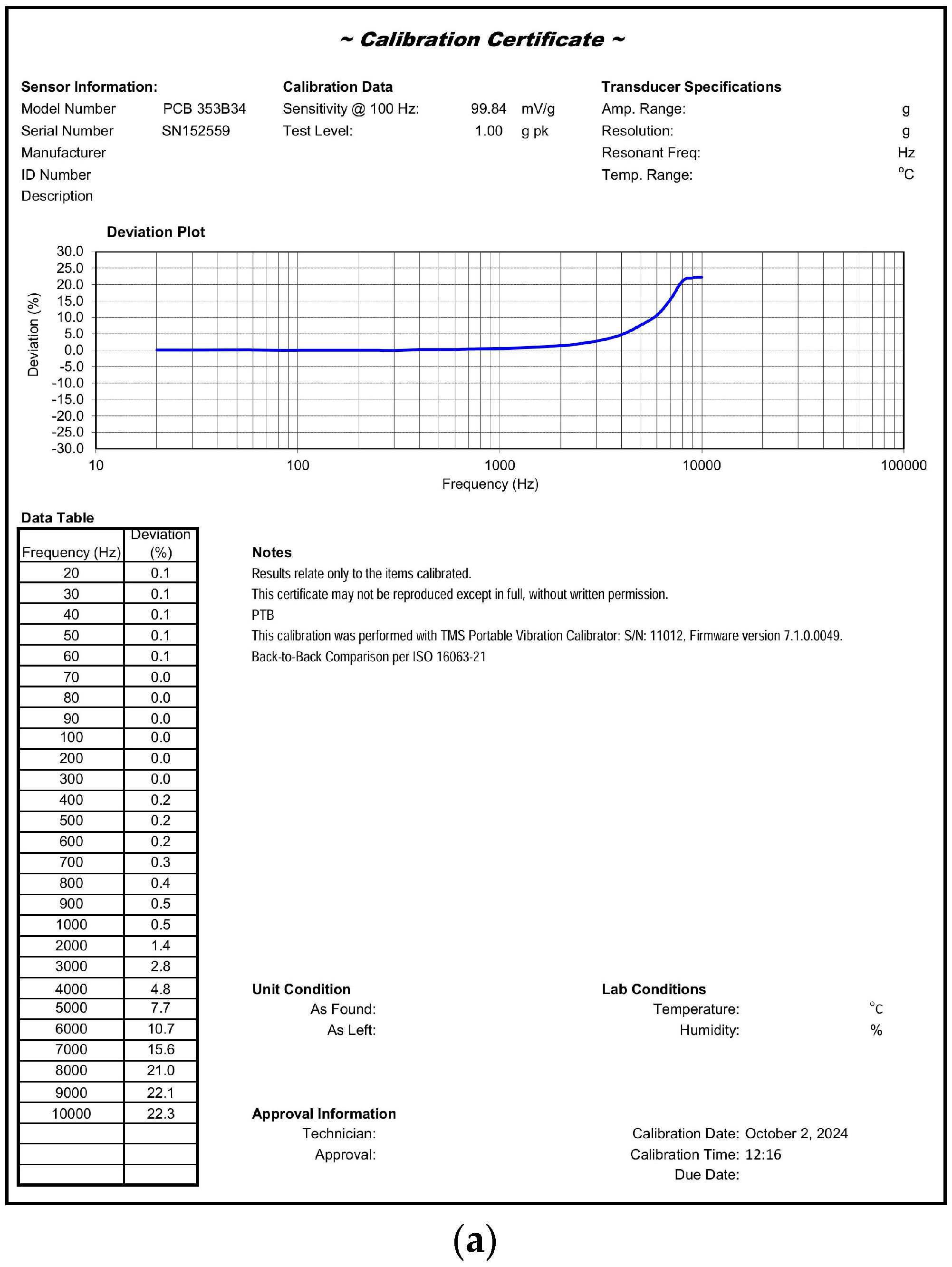
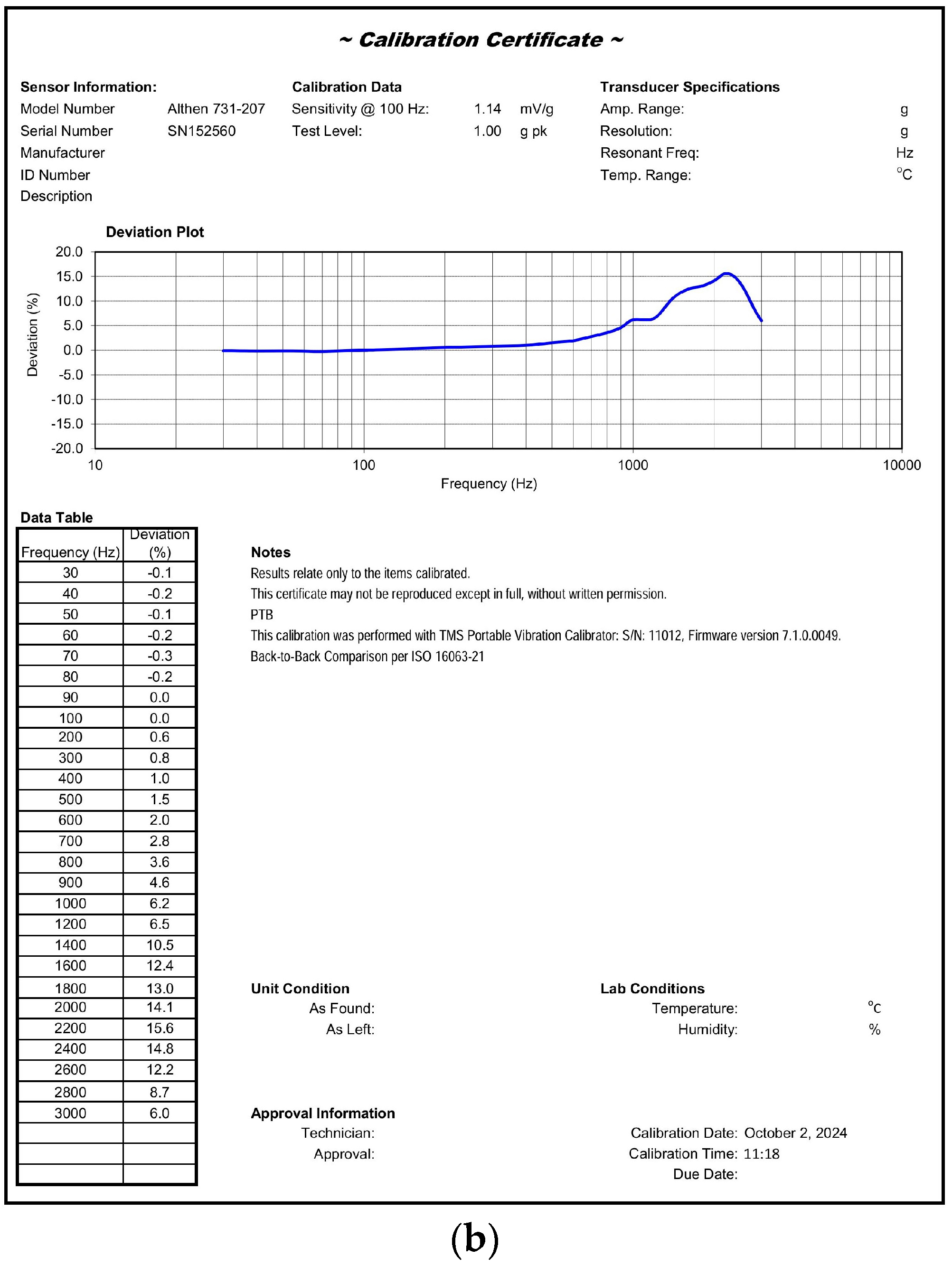
As an example of a practical experiment, two sensors were tested: the PCB 353B34 and Althen 731–207 accelerometers. The PCB 353B34 accelerometer was tested with a step of 10 Hz up to a frequency of 100 Hz, with a 100 Hz step up to a frequency of 1 kHz, and finally with a 1 kHz step up to a frequency of 10 kHz. The Althen 731–207 accelerometer was tested up to a frequency of 1 kHz with the same steps as for the PCB 353B34 accelerometer, while in the frequency range above 1 kHz, the step was 200 Hz. For both accelerometers, the sensitivity and deviation values were determined for the 27 frequency values of the input excitation signal at a constant amplitude of 1 g/pk.

Figure 3 shows the calibration certificates obtained for the PCB 353B34 (Figure 3a) and Althen 731–207 (Figure 3b) accelerometers. Both deviation characteristics are presented on a logarithmic scale here due to the wide range of frequencies considered for the input excitation signal.

The 5% deviations of the amplitude–frequency responses given in the corresponding datasheets for the PCB 353B34 and Althen 731–207 accelerometers are equal to 4 kHz and 650 Hz, respectively [26,27]. The certificate calibrations in Figure 3 confirm that for PCB 353B34, the 5% deviation of the above response exactly corresponds to the value declared in the datasheet, while for the Althen 731–207 accelerometer, the 5% deviation is equal to 900 Hz. This means that both accelerometers are functional and can be approved for further use.

Figure 3. Calibration certificates for the PCB 353B34 (a) and Althen 731–207 (b) accelerometers [28].

Figure 3. Calibration certificates for the PCB 353B34 (a) and Althen 731–207 (b) accelerometers [28].

The calibration results obtained using the portable calibrator shown in Figure 3 only allow us to determine or confirm the frequency response of the tested accelerometers. Using this calibrator, measurement points corresponding to the amplitude–frequency response of the accelerometers are also obtained. However, in order to determine all three parameters included in the transfer function given by Equation (3), it is proposed to use a procedure based on the Levenberg–Marquardt algorithm.

In order to determine the parameters of the model given in Equation (3) for both accelerometers, the procedure was used in accordance with Equations (13) and (14) based on the measured data presented in Figure 3. Figure 4 shows the regression results for the amplitude–frequency responses for the PCB 353B34 and Althen 731–207 accelerometers. This regression is presented on a logarithmic scale in the same way as the calibration certificates in Figure 3.

When implementing the Levenberg–Marquardt procedure, the following assumptions were made:

–

The initial values of the parameters $S_{\mathrm{k}},{ f}_{\mathrm{r}}$, and ${\mathrm{p}}_{\mathrm{r}}$ were set to 100 mV/g, 9 kHz, 123 mV/g and 1.14 mV/g, 2.2 kHz, and 1.33 mV/g for the PCB 353B34 and Althen 731–207 accelerometers, respectively;

–

The initial value of the parameter $\mu$ was set to $0.05$;

–

The value of parameter $\alpha$ was set to two.

Transforming the amplitude–frequency response into a function of the parameters $S_{\mathrm{k}},{ f}_{\mathrm{r}}$, and ${\mathrm{p}}_{\mathrm{r}}$ rather than the parameters $S_{\mathrm{k}},{ f}_0$, and $\beta$ makes the Levenberg–Marquardt procedure both easy to initialize and, more importantly, effective. This is due to the ease of estimating the initial values of the parameters $S_{\mathrm{k}},{ f}_{\mathrm{r}}$, and ${\mathrm{p}}_{\mathrm{r}}$ based on the measurement points of the amplitude–frequency response.

We denote the parameters of the models obtained for the accelerometers as ${\tilde{S}}_{\mathrm{k}},$ ${\tilde{f}}_{\mathrm{r}}$, and ${\tilde{p}}_{\mathrm{r}}$. The values of these parameters are 99.8 mV/g, 9898 Hz, 122.6 mV/g and 1.14 mV/g, 2.2 kHz, and 1.32 mV/g for the PCB 353B34 and Althen 731–207 accelerometers, respectively.

Figure 5 shows the relationship between the relative error given by Equation (15) and the frequency $f$ for the PCB 353B34 and Althen 731–207 accelerometers.

In Figure 5, it can be seen that the highest regression inaccuracy of the amplitude–frequency response occurs for values of the frequency f of 8 kHz for the PCB 353B34 accelerometer and 3 kHz for the Althen 731–207.

The mean square error (MSE), which represents the accuracy of the regression of measurement points, was determined based on the following relation:

$$\mathrm{M}\mathrm{S}\mathrm{E}={\displaystyle \frac{1}{N}}\sum _{n=1}^N{\left[A_n-A(f,{\tilde{S}}_{\mathrm{k}},{\tilde{f}}_{\mathrm{r}},{\tilde{p}}_{\mathrm{r}})\right]}^2$$

(16)

where $A$ denotes the measurement data.

The values obtained for the MSE were equal to 0.241 $\mathsf{\mu }\mathrm{V}/\mathrm{g}$ and 53.9 $\mathsf{\mu }\mathrm{V}/\mathrm{g}$ for the PCB 353B34 and Althen 731–207 accelerometers, respectively. We recalculated the parameter values ${ \tilde{f}}_0$ and $\tilde{\beta }$ for both accelerometers based on the parameter values ${\tilde{f}}_{\mathrm{r}}$ and ${\tilde{p}}_{\mathrm{r}},$ using Equations (10) and (11) and obtained ${ \tilde{f}}_0$ = 12.98 kHz and $\tilde{\beta }$ = 0.457 for the PCB 353B34 and ${\tilde{f}}_0$ = 3.12 kHz and $\tilde{\beta }$ = 0.502 for the Althen 731–207.

The results of accelerometer modeling obtained by applying the Levenberg–Marquardt procedure offer a basis for the implementation of other methods in the field of measurement signal processing. As an example, the implementation of the deconvolution method aimed at eliminating the dynamic error is presented below. This method can be implemented numerically by using the selected mathematical and computational program (MATLAB or MathCad). In engineering practice, convolutional filters [29] are used for this purpose to eliminate the dynamic error. However, the advantage of the numerical solution presented in this paper may be the possibility of implementing a filter (e.g., by using a signal processor system) dedicated to a specific accelerometer based on the modeling results obtained by applying the Levenberg–Marquardt algorithm.

By representing Equation (3) in the form of the equations of state, we have the following:

$$\mathbf{A}=\left[\begin{array}{cc}0& 1\\ -{\left(2\mathsf{\pi }{f}_0\right)}^2& -4\mathsf{\pi }{f}_0\beta \end{array}\right],\hspace{1em}\hspace{1em}\mathbf{B}=\left[\begin{array}{c}0\\ S_{\mathrm{k}}{\left(2\mathsf{\pi }{f}_0\right)}^2\end{array}\right].$$

(17)

The algorithm for deconvolution of the input signal in digital form, after quantization of the accelerometer output signal $y\left(t\right)$ to its digital equivalent $y\left[n\right]$, has the following form [29]:

$$\tilde{x}[n]={\displaystyle \frac{1}{{\Psi }_1}}\left(y[n+1]-{\phi }_{\mathrm{1,1}}y\left[n\right]-{\phi }_{\mathrm{1,2}}{y}_2\left[n\right]-...-{\phi }_{1,m}{y}_m\left[n\right]\right),$$

(18)

where

$$\begin{array}{c}{y}_2\left[n+1\right]={\Psi }_1\tilde{x}\left[n\right]+{\phi }_{\mathrm{2,1}}y\left[n\right]+{\phi }_{\mathrm{2,2}}{y}_2\left[n\right]+...+{\phi }_{2,m}{y}_m\left[n\right],\\ ⋮\\ y_m\left[n+1\right]={\Psi }_m\tilde{x}\left[n\right]+{\phi }_{m,1}y\left[n\right]+{\phi }_{m,2}{y}_2\left[n\right]+...+{\phi }_{m,m}{y}_m\left[n\right].\end{array}$$

(19)

The estimate $\tilde{x}\left[n\right]$ is obtained based on the parameter $y\left[n\right]$ with steps equal to $n$ and $n+1$, while the auxiliary parameters $y_2\left[n\right], ..., y_m\left[n\right]$ are obtained with a step equal to $n-1.$ The initial value of the parameter $y_2\left[n\right]$ is assumed to be equal to zero.

The matrix $\mathsf{\Psi }$ is calculated using the following equation:

$$\mathsf{\Psi }={\mathbf{A}}^{-1}\left(\mathsf{\Phi }-\mathbf{I}\right)\mathbf{B},$$

(20)

where

$$\mathsf{\Phi }={\mathrm{e}}^{\mathbf{A}\mathsf{\Delta }}$$

(21)

and

$$\mathbf{I}=\left[\begin{array}{cc}1& 0\\ 0& 1\end{array}\right]$$

(22)

is the identity matrix, while $\mathrm{e}$ and $\mathsf{\Delta }$ are the base of the natural logarithm and the step for quantization of the time $T$, which corresponds to the accelerometer testing time.

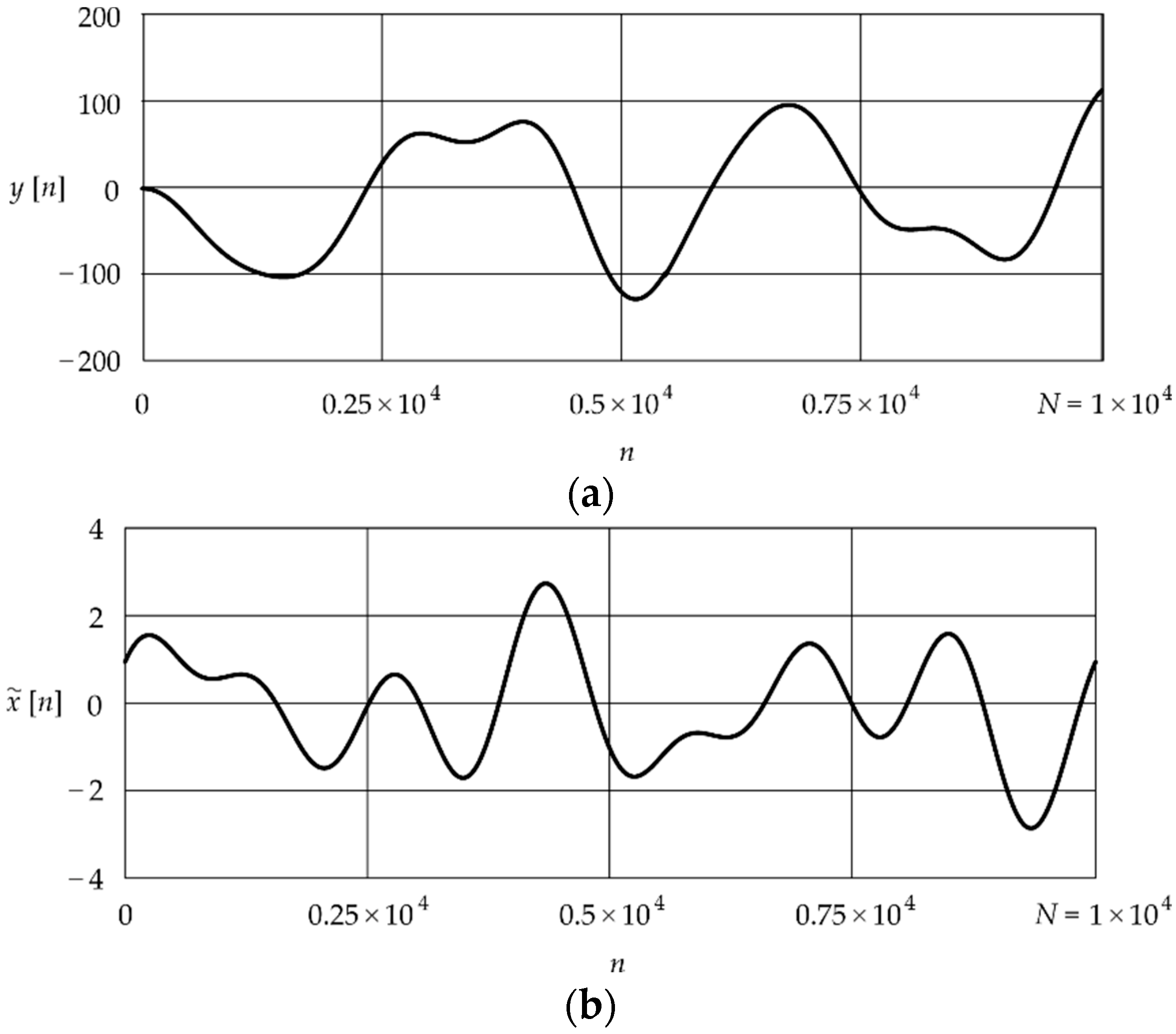
Figure 6 shows the input–output signals obtained by applying the deconvolution algorithm given in Equations (18) and (19) for the modeling results calculated for the PCB 353B34 accelerometer. Figure 6a shows the digital signal $y\left[n\right]$ recorded at the accelerometer output, while Figure 6b shows the digital signal $x\left[n\right]$ at the input of the accelerometer, obtained by using the deconvolution procedure.

The results of implementing the deconvolution algorithm presented in Figure 6 show that by modeling the accelerometer using the Levenberg–Marquardt procedure, it is possible to easily and effectively eliminate the dynamic error resulting from the non-ideal amplitude–frequency response for the frequency range of an accelerometer, i.e., one that does not have a constant value of the amplification factor for this range. The deconvolution algorithm allows for the reconstruction of the shape of the signal at the accelerometer input based on the signal recorded at its output.

4. Conclusions

This paper describes the application of the Levenberg–Marquardt procedure for modeling accelerometers intended for applications in the energy industry. An example illustrating the modeling of two selected accelerometers, PCB 353B34 and Althen 731–207, has been presented. The research results obtained here indicate the high effectiveness of the proposed procedure and demonstrate that it offers an alternative to the Monte Carlo method, which requires the use of pseudorandom generators and has a major disadvantage in terms of significant computational time. This is due to the fact that in the proposed solution, the parameters of the accelerometer model, which are the initial parameters for the Levenberg–Marquardt procedure, are determined with considerable accuracy based on the measurement points of the amplitude–frequency response.

As a result of applying the Monte Carlo method, the values obtained for the parameters ${\tilde{S}}_{\mathrm{k}},$ ${ \tilde{f}}_0$, and $\tilde{\beta }$ were 2% lower, 5% higher, and 1% lower for the PCB 353B34 accelerometer, respectively. For the Althen 731–207 accelerometer, the values of these parameters were 3% lower, 4% lower, and 2% higher, respectively. These differences are due to the random nature of the Monte Carlo method and to the iterative way of performing calculations in the Levenberg–Marquardt procedure.

The solutions presented in this paper are based on the results of accelerometer calibration obtained using practical experiments and may constitute a basis for further theoretical research in the field of the optimization of mathematical models of accelerometers and for practical research on eliminating the influence of the dynamic error in order to increase the accuracy of this type of sensor.