Efficient Approximation Procedure for Magnetization Characteristics Used in Performance Analysis of Highly Saturated Electrical Machines

Abstract

The analytical and especially the numerical calculations of the magnetic fields of highly saturated electrical machines require a correctly given magnetizing curve. In practice, professional software may use many points of the magnetizing curve (sometimes 50 or more points). There is a high probability that a point will be entered or measured incorrectly. We have therefore set ourselves three objectives. The first is to reduce the number of points given. The second is to ensure that the curve is given analytically (in the form of orthogonal polynomials) and is as smooth as possible. This means that the derivatives of the reluctance are also as smooth as possible. Therefore, the Newton–Raphson iteration procedure in numerical calculations converges rapidly. The third objective was to make the magnetizing curve continue beyond a magnetic field density of 2 T up to about 3 T. Most professional programs simply limit the magnetizing curve to about 2.2 T. This limitation makes it impossible to calculate accurately the magnetic field in the bridges, especially when the slots in the rotor are closed. Local fields can exceed values of 2.2 T. A solution has been found. It uses higher order orthogonal polynomials. It has been shown that 12 given points of the magnetizing curve is enough to give a good approximation of the measured curve. However, one polynomial function is not enough. We need three functions and another exponential function for magnetic field densities above around 2 T up to a value of relative permeability equal to 1. In the numerical calculation of the field, we thus achieve the desired error (residual) vector of the Newton–Raphson iterative procedure in 10 ÷ 15 steps for semi-closed slots and 20 ÷ 30 steps for closed slots.

1. Introduction

Producers of electric steel give us informative magnetic properties including three standard points, i.e., polarization J for alternating magnetic field strength data H = 2500, 5000 and 10,000 A/m. In the catalog of a producer, the magnetic properties, i.e., losses and polarization are shown in tables (discrete) and/or by curves. These data are the results of measurements of middle values between the rolling and transverse direction of magnetization with a single-sheet or Epstein measurer. The measurements depend on material quality and are given to 1.65 T or the largest value (about 1.95 T) at the frequency 50 Hz. Nowadays, these data are not enough to calculate the characteristics of highly saturated electrical machines, a point that is especially true of water-cooled AC servo motors.

The main difficulty is that the data points are done discretely, and the designers use them in their own or commercial software to define B–H characteristics. Most software uses numerical data points, most frequently the FEM, or analytical calculation. The problem is local saturation, which appears in all types of electrical machines.

The calculation time required to analyze a magnetic flux density above 2 T is extended, and the Newton–Raphson iteration procedure of the numerical calculations converge very slowly or do not converge at all. The results are often wrong. Commercial software allows the input of a limited number of data points for use in material definition, i.e., the magnetizing curve B = f(H). To eliminate the above-mentioned problems, we present in this article a method by which the suitable B–H characteristic to relative permeability µ_r = 1 at the upper boundary 2.2 ÷ 2.8 T can be determined. One advantage of the method proposed in this article is that it can be used for the numerical or analytical calculation of the characteristics of highly saturated electrical machines. In this article, the applicability of this method is demonstrated using two compressor-driven induction motors as examples.

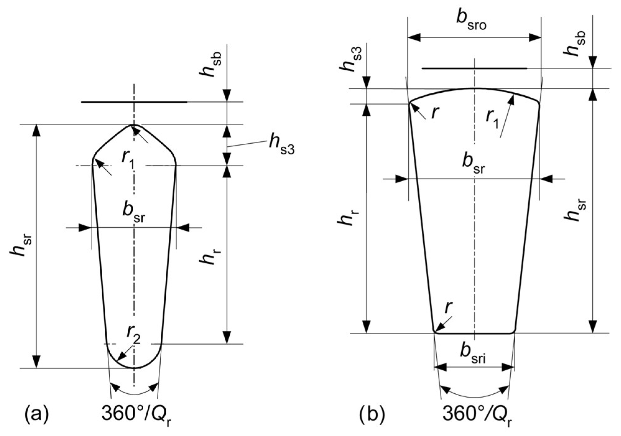
Induction motors in this type of application usually have a truncated stator lamination and closed rotor slots. This type of rotor lamination causes difficulties in magnetic field calculations applied to induction motors by means of numerical solution techniques. The value $h_{\mathrm{sb}}$ (Figure 1) of the rotor slot bridge is between 0.2 and 0.4 mm, and the value of the magnetic flux density in this region is over 2 T [1]. 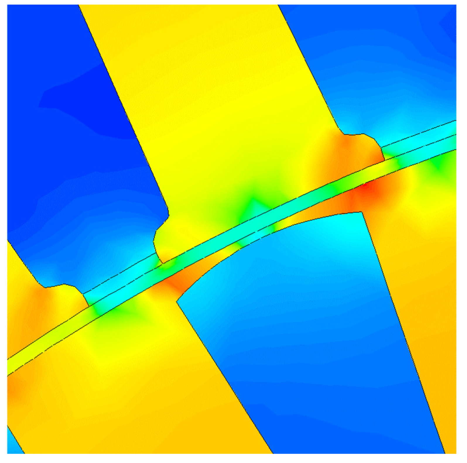Figure 2 presents the magnetic flux density distribution around the closed rotor slot of a three-phase induction motor at its rated load. Therefore, the magnetization characteristics, calculated reluctivities, and their derivatives as used for numerical magnetic field calculation in this region have to be smooth in order that the solutions calculated using the Newton–Raphson technique can converge.

This paper presents an algorithm for computation of the reluctivity and its derivative in order to avoid undamped oscillations of numerical field calculations due to the presence of such slots in induction motor rotor laminations. The algorithm was successfully employed in the software package emLook version 5.0 [2], designed for the computer-aided design of induction motors, synchronous motors, DC, and universal brush motors. Figure 1 shows two typical closed rotor slots for (a) a single and (b) a three-phase compressor motor from emLook’s database [2].

From the first attempts to make numerical calculations of the magnetic field, many authors have attempted to make sense of the magnetizing curve or its reluctivity in the form of an algebraic relation [3]. With today’s modern computer software packages, a tabulated magnetizing curve is incorporated into the package and interpolation between the actual data points is employed. Furthermore, magnetic anisotropy and lamination cutting technology [4,5] significantly impact the shape of actual magnetizing curves. This impact is significantly more prominent if the lamination’s tooth width is less than 5 mm. Therefore, some authors attempt to measure the resulting magnetizing curve from the manufactured iron core, which may be applicable to, e.g., inductor or transformer cores [6], but is not applicable to in rotation machines. There, the result also depends on the stator/rotor slots combination. In the article referenced herein as [7], the writers consider the impact of different processes of lamination manufacture and assembly on magnetic steel.

Some of the authors of previous works also analytically define approximated B–H characteristics based on measurement results: an analytical definition using only one equation [8,9], a piecewise approximation using three different equations [10], and the optimization of ferromagnetic characteristics to reduce Newton iterations [11]. But there is no solution to extrapolate values from the measured B–H characteristics (over 2 T), which is also needed in numerical calculations. This paper presents an algebraic procedure of attaining high order polynomial splines and their usage in an exemplary induction motor problem. The described method offers solutions to the following engineering problems, which exist in many electrical rotating machines with closed and semi-closed slots:

−

The approximation of measured magnetic characteristics where piecewise different mathematical functions are applied so that the measured and approximated curves are matched as closely as possible. The segmented functions are smoothly joined under the condition that their boundaries are matched, which results in a smooth approximated magnetization curve, which is applicable to the numerical analysis of highly saturated electrical machines. By applying the proposed technique, convergence problems in numerical analysis can be avoided.

−

The extrapolation of data into the region where measured data usually do not exist (2.0 T and more). By applying the proposed technique, more accurate calculations of electromechanical characteristics with numerical techniques for highly saturated motors are possible.

2. Construction of Non-Linear Magnetization Characteristic

In the year 1957, Forsyth [12] constructed an optional system of n data points x: x₁, ..., x_n and their values f(x): y₁, ..., y_n as orthogonal polynomials with three-links recursive relations. The orthogonal polynomials for the system of n points x₁, ..., x_n [13] are:

$$p_0(x), p_1(x), p_2(x)....$$

(1)

where the polynomial p_k(x) has the k-th degree. The polynomials are constructed in the form of (2):

$$p_{\mathrm{k}+1}(x)=(x-{\alpha }_{\mathrm{k}})p_{\mathrm{k}}(x)-{\beta }_{\mathrm{k}}{p}_{\mathrm{k}-1}(x), k=0, 1, ....$$

(2)

At the start, the first polynomial is: p₀(x) = 1, β₀ = 0. The coefficients for high order polynomials are found in the formulas of (3) and (4):

$${\alpha }_{\mathrm{k}+1}=\left({\displaystyle \sum _{i=1}^n{x}_{\mathrm{i}}{p}_{\mathrm{k}}^2(x_{\mathrm{i}})}\right)/\left({\displaystyle \sum _{i=1}^n{p}_{\mathrm{k}}^2(x_{\mathrm{i}})}\right)$$

(3)

$${\beta }_{\mathrm{k}}=\left({\displaystyle \sum _{i=1}^n{p}_{\mathrm{k}}^2(x_{\mathrm{i}})}\right)/\left({\displaystyle \sum _{i=1}^n{p}_{\mathrm{k}-1}^2(x_{\mathrm{i}})}\right)$$

(4)

The polynomial of order m is obtained from data points in the formula of (5) with the help of the minimum square method:

$$g(x)=a_0{p}_0(x)+.....+a_{\mathrm{m}}{p}_{\mathrm{m}}(x)$$

(5)

If the polynomials are orthogonal, the coefficients are in the form of (6):

$$a_{\mathrm{j}}=\left({\displaystyle \sum _{i=1}^n{y}_{\mathrm{i}}{p}_{\mathrm{k}}(x_{\mathrm{i}})}\right)/\left({\displaystyle \sum _{i=1}^n{p}_{\mathrm{j}}^2(x_{\mathrm{i}})}\right),j=0, 1, 2, ....,m$$

(6)

Equation (5) could be transferred in the final form of (7):

$$g(x)=a_0+a_{1}x.....+a_{\mathrm{m}}{x}^{\mathrm{m}}$$

(7)

In regions where the magnetic flux density is around 2 T, it was elaborated that the best solution for the approximation curve H = f(B) is an exponential function with two coefficients in the form of (8):

$$g(x)=a_{\mathrm{n}} x^n$$

(8)

3. Method for Determination of the Approximation Curve

The procedure to determine an adequate approximation curve H = f(B), which correlates the magnetic field strength H with the corresponding magnetic flux density B, is described for the laminated electrical steel quality type M800-50A.

Table 1. Standard values of electrical steel quality type M800-50A.

Designation by	Rated Thickness	Losses at 1.5 T Max.	Magnetic Polarization (T) (min.) for Alternating Magnetic Field Strength $\mathit{H}$ (A/m)			Anisotropy of Re-Magnetization Losses
EN 10027-1	(mm)	(W/kg)	2500	5000	10,000	% (max.)
M800-50A	0.50	8.00	1.60	1.70	1.78	±10

shows the minimum values of magnetic polarization and maximum values of losses for this type of steel, according to standard EN 10027-1 [14].

Many computer tests have revealed that a minimum of 12 prescribed measured points is needed in order to construct a smooth and adequate approximated magnetization curve for laminated electrical steel. However, only ten measured points are needed to construct an adequate approximation of the magnetization curve for a shaft of steel or machine housing. The advantage of using a minimal set of data points is a lower probability of inputting incorrect data values. Moreover, the polynomial order is also reduced by using a minimal set of data points. The manufacturer of electrical steel quality type M800-50A has provided 21 data points measured with an Epstein apparatus. Therefore, we selected only 14 measured data points to obtain 12 approximated (prescribed) standard data points to calculate the polynomials of the magnetization curve. The selected measured 14 data points are presented in

Table 2. Measured magnetization characteristics of electrical steel quality type M800-50A.

$\begin{array}{l} H\cdot {10}^2\\ (\mathrm{A}/\mathrm{m})\end{array}$	1.42	1.78	2.03	3.41	5.53	10.0	17.0	21.5	40.0	70.0	135.0	177.6	230.0	302.0
$B \left(\mathrm{T}\right)$	0.9	1.094	1.20	1.399	1.503	1.6	1.67	1.7	1.8	1.89	2.01	2.055	2.085	2.105

.

Some manufacturers provide catalog values B = f(H) for the following values of magnetic field strength: H = 500, 1000, 2500, 5000, 10,000, and 30,000 A/m. However, this set of data points does not suffice for the approximation of a smooth curve. Therefore, some data points are added to the standardized ones (

Table 3. Approximated data of magnetization characteristics.

$H\cdot {10}^2 (\mathrm{A}/\mathrm{m})$	1.6	2.0	2.5	4.0	6.5	10.0	16.0	25.0	50.0	100.0	200.0	300.0
$B \left(\mathrm{T}\right)$	1.0097	1.1872	1.2889	1.4365	1.5315	1.60	1.662	1.7254	1.8368	1.9563	2.0688	2.1051
$B^{*} \left(\mathrm{T}\right)$	1.00	1.165	1.294	1.43	1.528	1.60	1.664	1.72	1.835	1.958	2.065	2.105

* Calculated values, bold values are usually given by steel manufacturers.

).

Twelve interpolated data points of magnetic flux density B (shown in Table 3) are calculated from the 14 measured data points and using Equation (8) for interpolation. In order to estimate the errors of the measured interpolated points, the magnetization curve from Table 2 is plotted (Figure 3) and the values of magnetic field density B are interpolated at the prescribed values of magnetic field strength H (Table 3).

From the plotted magnetization curve, points marked with an * (Table 3) are calculated. These points have very small differences compared to the interpolated values, which demonstrates a good interpolation. While the plotting of the magnetization curve is quite time consuming, it reveals measurement errors. A comparison of the minimal standard values of B at H = 2500, 5000, and 10,000 (A/m) from Table 1 and the (bold) values from Table 3 shows that the manufacturer usually attains much higher values than those shown in Table 1. From the given data, the magnetization characteristic is initially constructed as a straight line up to the value of $B=1.103 \mathrm{T}$. Then the characteristic is constructed using three different orthogonal polynomials in the form of (7) with a maximum exponent of $m=5$, and after the value of the magnetic flux density $B=1.9525 \mathrm{T}$ is calculated, the approximation curve is exponential and dependent on the form of (8). Three orthogonal polynomials are needed to approximate the curves of high-permeability electrical steel or semi-finished electrical steel. The latter exhibits high variation in the curve knee region, and therefore an approximation with fewer polynomials does not suffice, although it is possible to calculate an approximation using only one polynomial in the curve’s middle region.

The orthogonal polynomials are calculated from the condition that the reluctivity derivative ($\partial {\nu }_1/\partial B=\partial {\nu }_2/\partial B$) in the margin point between two polynomials has to be equal for both polynomials. In other words, the derivative has to be continuous, i.e., without any pulsation. Otherwise, the Newton–Raphson iteration procedure used in the numerical calculations does not converge rapidly. The same is also valid for the connection between the straight line and the first polynomial, as well as for the connection between the exponential function and the third (last) polynomial. In the procedure used to calculate the polynomials, the values of the magnetic field strength are given in A/cm. Next, their decadal logarithm is calculated, and from these values the coefficients for the polynomials in the formula of (7) are calculated by using (3), (4), and (6).

Table 4. Coefficients for orthogonal polynomials.

B (T) >	B (T) ≤	a0	a1	a2	a3	a4	a5
1.0617	1.5665	0.1071788 × 103	−0.4110740 × 103	0.6262400 × 103	−0.4730883 × 103	0.1771756 × 103	−0.2622590 × 103
1.5665	1.7484	0.3622065 × 104	−0.1033155 × 105	0.1175909 × 105	−0.6678794 × 104	0.1893319 × 104	−0.2143522 × 103
1.7484	2.0970	−0.8258395 × 102	0.16644346 × 103	−0.1268026 × 103	0.4371245 × 102	−0.5666790 × 101	0

presents the coefficients for three orthogonal polynomials in three different regions of the values of B. The exponential function in the region above $B>2.097 \mathrm{T}$ has been determined as (9).

$$g(x)=0.5164848 x^{2.033383}$$

(9)

By using this procedure, the output values presented in

Table 5. Output values $H=f(B)$ and ${\mu }_{\mathrm{r}}=f(B)$.

$H\cdot {10}^2 (\mathrm{A}/\mathrm{m})$	1.6	2.0	2.5	4.0	6.5	10	16	25	50	100	200	300
$B \left(\mathrm{T}\right)$	1.0417	1.1876	1.2892	1.4366	1.5324	1.6001	1.6621	1.7257	1.8375	1.9569	2.0820	2.1620
${\mu }_{\mathrm{r}}$	5181	4725	4104	2858	1876	1273	826.82	549.3	292.5	155.7	82.85	57.35

were calculated for input points of the B–H curve shown in Table 3.

With the exponential approximation curve H = f(B) in the form of (9), a relative permeability µ_r = 1 is reached for a value of magnetic flux density $B\approx 2.8529 \mathrm{T}$.

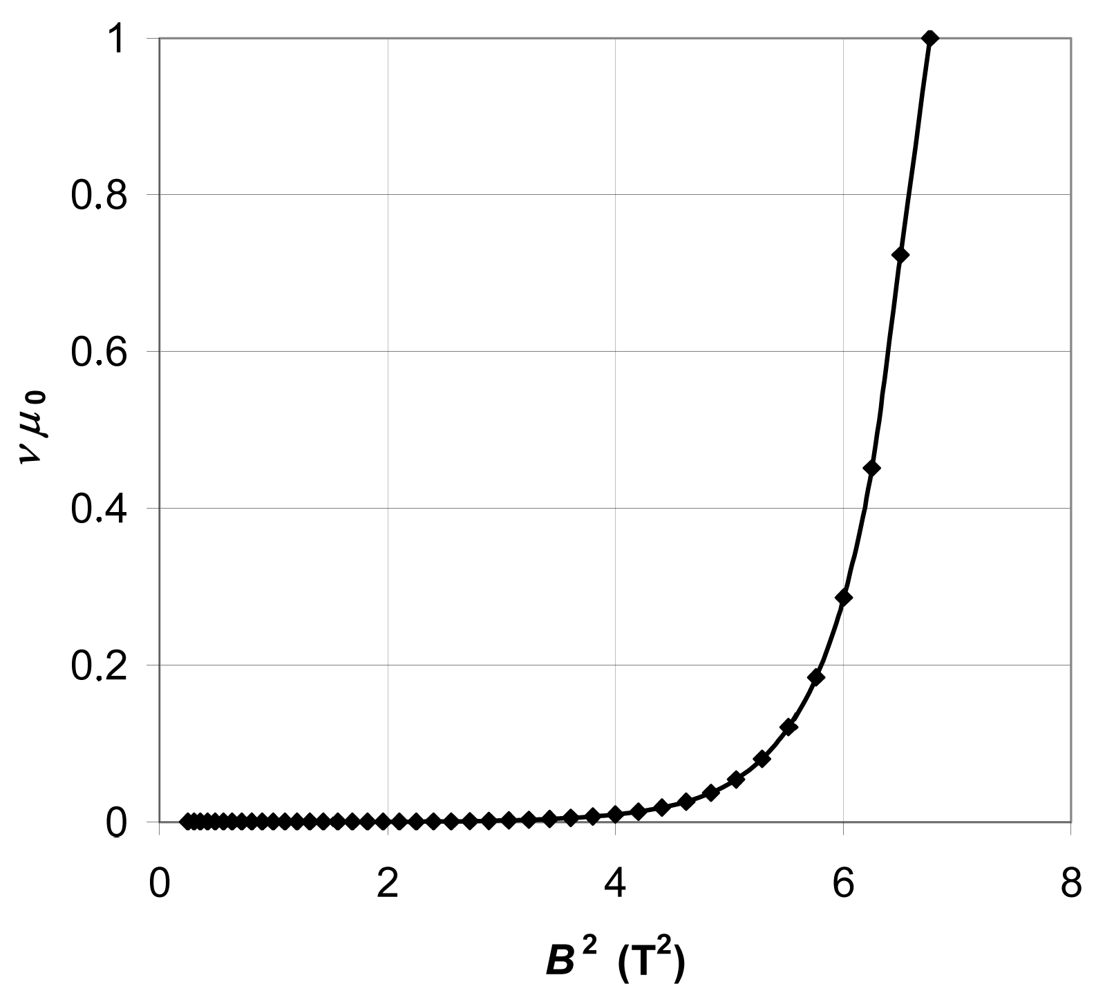
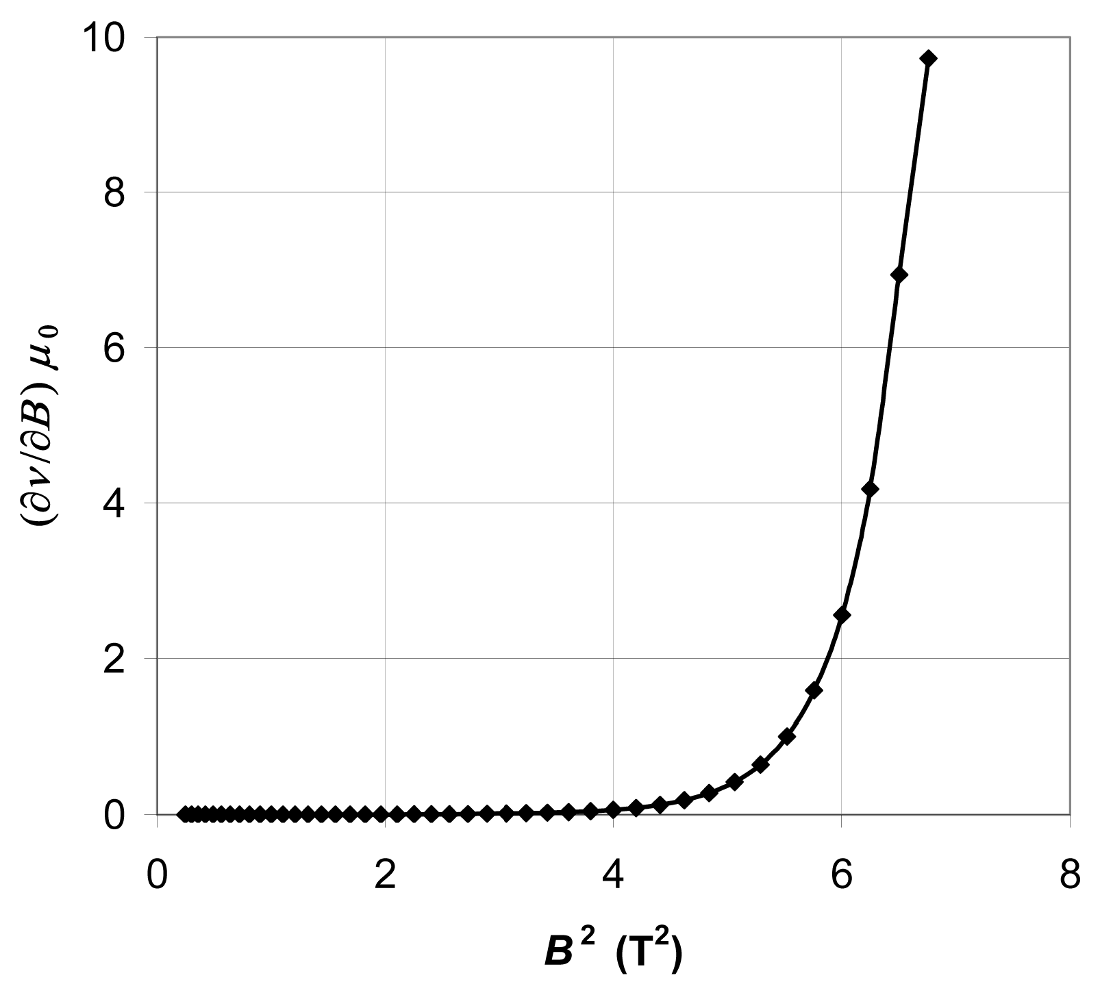
Figure 4 shows the approximated B–H curve and the measured data points. Figure 5 shows the modeled relative reluctivity and Figure 6 shows the reluctivity derivative. Both of the functions plotted in Figure 5 and Figure 6 are relatively smooth; therefore, convergence problems in the numerical calculation of the magnetic field should not arise.

Approximated B–H curves, their relative reluctivity and the reluctivity derivative, are used in the research software package emLook [2], which is designed for analytical calculation and variation of the characteristics of three-phase and single-phase induction motors and DC and universal brush motors. EmLook’s database contains 34 different predefined B–H curves, of which one may be easily selected by the users before they start the calculation of a magnetic circuit and its respective motor characteristics. Figure 7 shows a screenshot of the aforementioned B–H curve of a steel sheet of quality M800-50A. A special software module [2] enables the preparation of finite element analyses input data, like the dimensions of the stator and rotor lamination and the current densities in the stator and rotor windings, e.g., for the stator winding data of a three-phase compressor drive induction motor. Another module in [2] analytically calculates the initial current densities in stator slots and similarly for the squirrel-cage in rotor slots for further numerical calculations by utilizing the finite element method.

4. Usage of Approximated Magnetization Characteristics

Magnetization characteristics obtained by the previously described procedure have been used in the solution procedure of many (quasi-) static magnetic field problems dealing with electrical rotating machines. All problems could be solved more quickly (i.e., with fewer iteration steps) by using the smooth approximated magnetization characteristic as opposed to using the measured characteristic. However, in many cases, problems of electrical machines with closed slots indicated convergence problems. This is caused by the high saturation levels around the closed slot and the fact that manufacturers usually do not provide measured data above 2.0 T. Therefore, the magnetization characteristic has to be extrapolated to high values of magnetic field density in order to reach ${\mu }_{\mathrm{r}}=1$. Magnetic field calculations of a small single-phase induction motor with permanent split capacitor and closed rotor slots used for driving the compressor of a domestic refrigerator (230 V, 50 Hz, 88 W, 2860 rpm, 3 µF), have showed that in spite of high saturation in the rotor slot bridge area (width $b_{\mathrm{sr}}$ from Figure 1a), the main magnetic circuit was not highly saturated [1]. For the single-phase motor with closed rotor slots, the desired error between two steps $(\epsilon \le 0.5\cdot {10}^{-6})$ was achieved in 20 iteration steps. Meanwhile, for the semi-closed rotor slots version, the desired error was achieved in 12 iteration steps (

Table 6. Error (residuum) vector of Newton–Raphson iterative procedure for single-phase induction motors with closed and semi-closed rotor slots.

Step	Closed Rotor Slots Error Vector ε	Step	Semi-Closed Rotor Slots Error Vector ε
1	0.279566 · 100	1	0.214958 · 100
2	0.129734 · 100	2	0.121239 · 100
3	0.730933 · 10−1	3	0.683485 · 10−1
4	0.422006 · 10−1	4	0.385479 · 10−1
…	…	…	…
20	0.287574 · 10−6	12	0.479654 · 10−6

).

Magnetic field calculations for a larger three-phase induction motor (400 V, 50 Hz, 18 kW, 1430 rpm) with closed rotor slots (Figure 1b) have shown that the convergence achieves the desired error in 23 steps (where the Newton–Raphson iteration starts with an assumed zero-potential distribution), despite the fact that the whole machine’s cross-section is exposed to extreme saturation conditions. For the same motor with semi-closed rotor slots, the desired error was achieved in ten iteration steps (

Table 7. Error (residuum) vector of Newton–Raphson iterative procedure for three-phase induction motors with closed and semi-closed rotor slots.

Step	Closed Rotor Slots Error Vector ε	Step	Semi-Closed Rotor Slots Error Vector ε
1	0.143789 · 10+1	1	0.137036 · 10+1
2	0.675862 · 100	2	0.758043 · 100
3	0.211834 · 100	3	0.286215 · 100
4	0.111814 · 10−1	4	0.559355 · 10−1
…	…	…	…
23	0.121830 · 10−6	10	0.11011 · 10−6

).

The aforementioned calculations were carried out using our own research 2D finite element software package emLook version 5.0. Similar general relations and comparable results can be obtained by using (more) general purpose and commercially available solvers, which do not allow the integration of a polynomial function but merely a higher or lower number of data points representing a B–H curve. In the presented example, the incremental (differential) relative permeability equals ${\mu }_{\mathrm{r}}=1.0$ at $B=2.422 \mathrm{T}$, despite the fact that the approximation function gives a value of ${\mu }_{\mathrm{r}}\approx 13.2$ at the same value of B.

To sum up, we can state that if the magnetization characteristic, reluctivity, and their derivatives are smooth and extrapolated over 2 T, the Newton–Raphson technique also converges in the region of the extreme conditions of saturation, i.e., in the area around the closed rotor slot bridge, as described in the previous example. The calculation time achieved by applying the magnetizing curve in the form of orthogonal polynomials was some seconds. Using 24 measured points of the magnetizing curve lengthened the calculation time to some minutes. Furthermore, in cases of closed rotor slots the Newton–Raphson iteration procedure does not always converge.

Except for the approximation of the B–H curves of electric steel with orthogonal polynomials, this procedure can be used to approximate the hysteresis loop of electrical steel or the B–H curves of permanent magnets [13,15]. Using the transient calculation on the transformers at no-load is a problem at high saturation; our method could be used to solve this problem [16,17].

5. Conclusions

Some professional software requires up to 50 measurement points to provide a magnetizing curve. Such software uses interpolation to calculate the magnetic field strength, reluctance, and most essentially the reluctance derivative. This slows down the calculation of the magnetic field and raises the probability of errors in the input of the measured points. Therefore, a procedure is presented for an analytically given magnetizing curve using orthogonal polynomials and an exponential function. Such a magnetizing curve can be used to calculate a magnetic circuit with highly saturated bridge regions specifically for closed rotor slots. It is also possible to extrapolate the magnetic curve beyond 2 T, where magnetic characteristic measurements are no longer particularly accurate. This is achieved by using an exponential function defined by the data of the last two measured points. Such a magnetizing curve is very smooth, and therefore the Newton–Rapson iterative procedure converges rapidly. A maximum of 12 standard measurement points is needed to determine the magnetic curve. It is also possible to construct polynomial functions depending on the width “w” of each part of the magnetic circle H = f(B, w). In this way, the influence of the lamination punching or edge effect is taken into account. The magnetizing curve shown in this paper is thus given by a straight line from the origin magnetic field density from 0 T to 1.0617 T, with the three orthogonal polynomials up to 2.097 T and an exponential function over 2.097 T for electrical steel of the quality type M800-50A.