Impact of Energy System Optimization Based on Different Ground Source Heat Pump Models

Abstract

With rapidly developing new energy technologies, rational energy planning has become an important area of research. Ground source heat pumps (GSHPs) have shown themselves to be highly efficient. effective in reducing building or district energy consumption and operating costs. However, when optimizing integrated energy systems, most studies simplify the GSHP model by using the rated coefficient of performance (COP) of the GSHP unit, neglecting factors such as soil, buried piping, and actual operating conditions. This simplification leads to a deviation from the actual operation of GSHPs, creating a gap between the derived operational guidelines and real-world performance. Therefore, this paper examines a hotel equipped with photovoltaic panels, a GSHP, and a hybrid energy storage unit. By constructing models of the underground pipes, GSHP units, and pumps, this paper considers the thermal exchanger between the underground pipes and the soil, the thermal pump, and the operating status of the unit. The purpose is to optimize the running expenses using an enhanced mote swarm optimization (PSO) algorithm to calculate the optimal operating strategy of system equipment. Compared to the simplified energy system optimization model, the detailed GSHP unit model shows a 21.36% increase in energy consumption, a 13.64% decrease in the mean COP of the GSHP unit, and a 44.4% rise in system running expenses. The differences in the GSHP model affect the energy consumption results of the unit by changing the relationship between the power consumption of the PV system and the GSHP at different times, which in turn affects the operation of the energy storage unit. The final discussion highlights significant differences in the calculated system operating results derived from the two models, suggesting that these may profoundly affect the architectural and enhancement processes of more complex GSHP configurations.

1. Introduction

As the variety of load types and user-side demand increases, relying on fossil energy to meet these needs consumes substantial fossil resources, leading to resource reduction and severe environmental impacts [1]. The energy supply sector is proactively addressing the long-standing challenges associated with resource depletion and pollution. This is being achieved through the integration of a greater proportion of new clean energy into the energy supply, promoting the advancement of the low-carbon energy supply industry, and fostering a low-carbon economy [2,3,4]. Consequently, more buildings are complying with national policies by installing a minimum standard of renewable energy equipment [5]. This mandatory regulation effectively reduces fossil energy consumption and CO₂ emissions [6]. However, the rise of new energy-distributed generation systems has caused a surge in power generation, transforming the structure of electricity consumption in buildings into an energy local area network (ELAN) with demand-side participation and interaction. Thus, the efficient use of energy has become a crucial goal. According to the latest data, the building sector in the United States accounts for about 70% of electric energy consumption [7], with 41.4% of this consumption directly related to space heating, ventilation, and air conditioning. The energy consumed by air conditioning systems in buildings exhibits characteristics that offer considerable potential for energy savings and optimal energy scheduling. Ensuring user demand while optimizing equipment operation is crucial to reducing electricity costs for users, lowering peak electricity consumption and photovoltaic (PV) curtailment rate, and effectively reducing the peak-valley difference in the power grid.

Ground source heat pumps (GSHP) have recently attracted considerable interest due to their potential for high energy efficiency. The consistent soil temperature throughout the year allows GSHP systems to maintain stable and high operating efficiency, enhancing their regulation potential. Consequently, GSHPs have become essential sources of cooling and heating in integrated energy systems (IES) [8]. Yang et al. [9] utilized a two-layer optimal scheduling model to optimize IES containing GSHPs. This resulted in a notable augmentation in the system’s wind power consumption capacity and a concomitant reduction in operational costs. Gao et al. [10] conducted economic and optimal scheduling for an electric-thermal IES with GSHPs, optimizing system operations, reducing costs, and enhancing clean energy consumption capacity. Yang [11] applied mixed-integer programming to optimize an islanded micro-energy network with GSHPs, lowering system operating costs. Zhang et al. [12] used an improved Bald Eagle Search (BES) algorithm to tackle the issue of integrated energy systems with GSHPs across different seasons, developing varied energy supply scheduling strategies. Li et al. [13] employed a genetic algorithm to calculate hotel building equipment operations, using cost-saving rates and primary energy consumption-saving rates as comprehensive evaluation indexes, providing references for energy system configuration and appropriate operation strategies. Zeng et al. [14] optimized system equipment operations using a genetic algorithm with primary energy saving rate, CO₂ reduction rate, and annual total cost saving rate as optimization objectives, formulating the operation strategy with the lowest operation cost and CO₂ emissions. Ren et al. [15] conducted day-ahead optimal scheduling for GSHP energy systems with hybrid energy storage devices, demonstrating that this integrated approach significantly reduces operating costs and improves energy utilization compared to traditional heat and power distribution modes. Tao et al. [16] used the Gurobi solver to identify the optimal configuration, revealing that adding GSHP and energy storage systems to the setup significantly lowers annual CO₂ emissions. Currently, the primary design approach for GSHPs is a fixed capacity one, which does not take into account the operational characteristics of GSHPs under partial load conditions, nor the maintenance of resident comfort. Consequently, when optimizing the performance of integrated energy systems containing GSHPs, calculations are often based on the rated operating conditions of the ground source heat pumps. This approach neglects crucial factors such as soil temperature, buried pipe heat exchange, unit load rate, and other operational conditions. As a result, these calculations have limitations in effectively guiding the actual operation of GSHPs.

Due to the highly nonlinear nature of the ground source heat pump model and the need for nonlinear and discrete iterative calculations for ground temperature, the calculations are limited by numerous constraints. Therefore, a linear approach cannot be used for the optimization calculation of GSHP energy systems [17]. To address these challenges, an effective optimization method is needed to solve nonlinear physical phenomena. Scholars have found heuristic algorithms to be highly effective for computing nonlinear problems, such as the particle swarm optimization (PSO) algorithm [18,19], differential evolution algorithm (DE) [20], whale optimization algorithm (WOA) [21], Nelder–Mead method [22], dynamic programming [23], and genetic algorithm (GA) [24]. This paper presents an improved PSO algorithm for determining the optimal operation strategy for a GSHP system with a hybrid energy storage device under PV conditions, taking into account the dynamic changes in soil temperature and GSHP unit performance.

This paper aims to compare the optimal operation strategies of energy systems with ground source heat pumps using different GSHP models. A case study was conducted using a hotel building in Beijing as a model for the ground source heat pump. The model considered a range of factors, including soil conditions, buried pipe parameters, and the operation of water pumps. The improved particle swarm optimization (IPSO) algorithm was used to optimize the energy system, including the cold storage device, photovoltaic device, and GSHP. The optimal system operation strategy was identified through the minimization of the total daily operational cost, which was established as the objective function. This was achieved by considering the actual operational constraints, including those pertaining to equipment. Compared with the system energy planning strategy of the simplified model under the same calculation conditions, the operational differences of energy system equipment under different models were analyzed.

2. Modeling of Energy Systems

This paper addresses the energy system of a hotel building in Beijing, outlining a structural composition as illustrated in Figure 1. The GSHP is the primary source of cooling and heating for the building, fulfilling the majority of the building’s cooling and heating load requirements. In addition to the GSHP, the energy system includes PV panels and an energy storage system (for both cold and power storage), which work synergistically. The figure illustrates a schematic representation of the cold energy flow within the system, with the GSHP serving as a single source of refrigeration, providing cooling to the building. The load ratio of the GSHP can be adjusted by operating the cold storage device. The dotted line represents the direction of electric power flow within the system. There are three power supply channels for the GSHP: the PV components, the storage battery, and the power grid, all of which can supply power to the GSHP unit through an inverter. During the day, when there is sufficient electricity, the PV power generation system prioritizes meeting the electricity demand of the GSHP unit. Any surplus PV power generated is stored in the storage battery. In the event that the generation of PV power is insufficient to meet the energy demand of the GSHP unit, the demand is shared between the PV power and the grid.

2.1. Buried Pipe Model

In this paper, the buried pipe is a single U-shaped pipe designed to facilitate the conveyance of water. As the water within the pipe cools by releasing heat into the rock and soil, and then flows out the other end of the buried pipe. For the purposes of this analysis, the soil is posited to be a homogeneous, isotropic medium, semi-infinite. The pertinent parameters, including soil thermophysical properties and the configuration of the buried pipe, are provided in

Table 1. Calculation parameters.

Parameter	Value
Initial soil temperature (°C)	15
depth (m)	100
Drilling diameter (m)	0.08
Number of boreholes	49
inside diameter (m)	0.026
Thermal conductivity of pipe [W/(m·K)]	0.39
U-shaped tube thickness (m)	0.0024
outside diameter (m)	0.032
Water Specific thermal capacity [J/(kg·K)]	4181
Convective heat transfer coefficient of tube [W/(m2·K)]	3575

for reference.

The model outside the buried pipe borehole uses a wireline-long heat source model, assuming that the buried pipe is in a semi-infinite medium and that the soil is an infinite, homogeneous, and isotropic medium. The temperature of the soil at any point around a single buried pipe at time τ can be determined using the following analytical equation [25]:

$$\mathrm{T}(r,z,\tau )=T_0+{\displaystyle \frac{q_0}{4\pi k_s}}{\displaystyle {\int }_0^1\left[\frac{erfc(\stackrel{\sim +}{r}/2\sqrt{Fo})}{\stackrel{\sim +}{r}}-\frac{erfc(\stackrel{\sim -}{r}/2\sqrt{Fo})}{\stackrel{\sim -}{r}}\right]}d\zeta$$

(1)

$${\tilde{r}}^{+}=\sqrt{{\beta }^2+{(\eta -\xi )}^2}$$

(2)

$${\tilde{r}}^{-}=\sqrt{{\beta }^2+{(\eta +\xi )}^2}$$

(3)

where: T₀ represents the initial temperature of the fluid inside the buried pipe, and in this model, the soil temperature is set as the initial temperature, °C; q₀ denotes the heat flux per linear meter along the depth of the pipe well, expressed in W/m. k_s represents the thermal conductivity of soil, taken as k_s = 1.4 W/(m K); $\stackrel{\sim +}{r}$ represents the dimensionless distance parameter between the instantaneous point heat source in the line heat source and a certain point in the soil; $\stackrel{\sim -}{r}$ is the dimensionless distance parameter between the instantaneous point heat source in the virtual heat source and a certain point in the soil; η is the dimensionless depth parameter of a certain point in the soil; β represents the dimensionless distance parameter between a certain point in the soil and a linear heat source; ξ represents the dimensionless depth parameter at a certain point of the line heat source; erfc (z) is the residual error function, expressed as:

$$erfc(z)=1-2{{\displaystyle \int }}_0^{z}exp(-u^2)du/\sqrt{\pi }$$

(4)

Fo represents Fourier time, and its expression is as follows: $Fo=\tau \alpha /H^2$.

The g-function defines the instantaneous temperature response of a single borehole subjected to a step load within the framework of the restricted length line thermal source model:

$$g(\beta ,Fo)={{\displaystyle \int }}_0^1\left[{\displaystyle \frac{erfc({\tilde{r}}^{+}/2\sqrt{Fo})}{{\tilde{r}}^{+}}}-{\displaystyle \frac{erfc({\tilde{r}}^{-}/2\sqrt{Fo})}{{\tilde{r}}^{-}}}\right]d\xi$$

(5)

Chen et al. [26] defined in the literature the temperature reaction coefficient δ-function of the wall of a buried pipeline under rectangular heat flow with a time interval of Δτ. ΔFo is the Fourier number at the time interval Δτ. The wall of a buried pipeline is defined as follows:

$$\delta ({\beta }_b,Fo)=\overline{g}({\beta }_b,Fo)-\overline{g}({\beta }_b,Fo-\mathsf{\Delta }Fo)=-{{\displaystyle \int }}_0^{\mathsf{\Delta }Fo}{\overline{g}}_{Fo}^{\prime }({\beta }_b,Fo-\overline{x})dx$$

(6)

The δ-function at the wall surface of the buried pipe at any i(0 ≤ τ ≤ i) moments is obtained according to Equations (5) and (6):

$$\delta ({\beta }_b,F{o}_{j-i+1}-x)=-{\displaystyle \underset{0}{\overset{\mathsf{\Delta }Fo}{\int }}\frac{exp(-{\beta }_b^2/4F{o}_{j-i+1}-x)}{4Fo}\left[2-4erfc(\frac{1}{2\sqrt{F{o}_{j-i+1}-x}})+2erfc(\frac{1}{\sqrt{F{o}_{j-i+1}-x}})-A(F{o}_{j-i+1}-x)\right]dx}$$

(7)

where:

$$A(F{o}_{j-i+1}-x)=2\sqrt{F{o}_{j-i+1}-x}[exp(-{\displaystyle \frac{1}{F{o}_{j-i+1}-x}})-4exp(-{\displaystyle \frac{1}{4F{o}_{j-i+1}-x}})+3]/\sqrt{\pi }$$

(8)

When calculating the wall temperature of the kth buried pipe within a group of pipes, the temperature is influenced by multiple buried pipes. Therefore, it is necessary to superimpose the wall temperature response of the other buried pipes in the kth well to determine the temperature at the wall of the kth buried pipe well:

$$T_{b,k}(\tau )=T_0+{\displaystyle \frac{1}{2\pi k_s}}\left\{{\displaystyle \sum }_{i=1}^{\tau }{q}_0(i)\cdot {\mathsf{\Delta }}_k({\beta }_{all},F{o}_{\tau -i+1})\right\}$$

(9)

where Δ(β_all, Fo_τ−i+1) is the accumulation of the average temperature reaction factors of all buried pipes within the pipe group at wellbore facade of buried pipe k at time i.

$$\mathsf{\Delta }({\beta }_{all},F{o}_{r-i+1})=\delta ({\beta }_b,F{o}_{r-i+1})+{\displaystyle \sum }_{j=1}^{N-1}\delta ({\beta }_j,F{o}_{r-i+1})$$

(10)

The temperature response factor at buried pipe k at its wall at moment i and the temperature response factor of the remaining buried pipes at the wall of buried pipe k are first superimposed, i.e., the total temperature response factor of the buried pipe k wall at moment i can be calculated by Equation (10). Then, the historical heat flow and the total temperature response factor at the corresponding moment are calculated by convolving Equation (9) to find the temperature of the wall of the entombed pipe k pipe well.

To consider a quasi-3D in-borehole stable state thermal transfer model, the in-borehole model was adopted. This model considers the transfer of heat transfer between the transverse and longitudinal directions of the buried pipe, while ignoring the longitudinal thermal conductivity inside the borehole. The dimensionless energy balance equation for this model is given by [27].

$$T_{out}=T_b+{\displaystyle \frac{\beta S_1\cdot ch\beta -sh\beta }{\beta S_1\cdot ch\beta +sh\beta }}(T_{in}-T_b)$$

(11)

$$\beta =\sqrt{1/S_1^2+2/(S_1{S}_{13})}$$

(12)

$$S_1={\displaystyle \frac{M{c}_p}{H}}(R_{11}+R_{13})$$

(13)

$$S_{13}={\displaystyle \frac{M{c}_p}{H}}({\displaystyle \frac{R_{11}{}^2-R_{13}{}^2}{{\mathrm{R}}_{13}}})$$

(14)

$$R_{11}={\displaystyle \frac{1}{2\pi k_b}}\left[\ln ({\displaystyle \frac{r_b}{r}})-{\displaystyle \frac{k_b-k_s}{k_b+k_s}}\ln ({\displaystyle \frac{r_b^2-D^2}{r_b^2}})\right]+{\displaystyle \frac{1}{2\pi k_p}}\ln {\displaystyle \frac{r_o}{r_i}}+{\displaystyle \frac{1}{2\pi r_{i}h}}$$

(15)

$$R_{12}={\displaystyle \frac{1}{2\pi k_b}}\left[\ln ({\displaystyle \frac{r_b}{\sqrt{2}D}})-{\displaystyle \frac{k_b-k_s}{2(k_b+k_s)}}\ln ({\displaystyle \frac{r_b^4+D^4}{r_b^4}})\right]$$

(16)

$$R_{13}={\displaystyle \frac{1}{2\pi k_b}}\left[\ln ({\displaystyle \frac{r_b}{2D}})-{\displaystyle \frac{k_b-k_s}{k_b+k_s}}\ln ({\displaystyle \frac{r_b^2+D^2}{r_b^2}})\right]$$

(17)

where r_i is the interior diameter of the U-shaped pipe, m; r_o is the outer diameter of the U-shaped pipe, m; r_b is the distance from the center of the tube well, m; M is the mass flow rate of the fluid inside the pipe, kg/s; c_p is the convective thermal transfer factor of fluid inside tube, W/m²; k_p and k_b represent the thermal conduction of the U-shaped pipe and the thermal conduction of backfill material in the pipe well, respectively, W/(m·K).

In order to evaluate the proposed model, it was compared with the calculation results of the drill pipe model in TRNSYS18 software. The results are presented in Figure 2. The discrepancy between the calculated and observed values was found to be within an acceptable range.

2.2. Heat Pump Model

The thermal pump model is derived from the GHSP unit model provided in the DOE-2 software, where the energy consumption and COP of the unit are dependent upon the water flow rate, water temperature, and part-loading ratio. These parameters can be used to derive the energy consumption and COP of the GSHP unit using following equation [28]:

$$CA{P}_{\max }=CA{P}_0·CA{P}_r$$

(18)

$$CA{P}_r=a_1+b_1{r}_{me}+b_2{r}_{me}^2+c_1{r}_{mc}+c_2{r}_{mc}^2+d_1{r}_{reo}+d_2{r}_{Teo}^2+e_1{r}_{Tei}+e_2{r}_{Tei}^2+f_1{r}_{Teo}{r}_{Tei}$$

(19)

$$P_{GSHP}=P_0{P}_{r1}{P}_{r2}$$

(20)

$$P_{r1}=a_2+b_3{r}_{me}+b_4{r}_{mc}^2+c_3{r}_{mc}+c_4{r}_{mc}^2+d_3{r}_{reo}+d_4{r}_{reo}^2+e_3{r}_{Tri}+e_4{r}_{Tri}^2+f_2{r}_{Teo}{r}_{Tri}$$

(21)

$$P_{r2}=a_3+a_{4}PLR+a_{5}PL{R}^2$$

(22)

where CAP_max represents the maximum cooling capacity of the system under different operating conditions, taken as CAP_max = 275 kW; CAP₀ represents the cooling ability of the unit when it is working at full capacity under rated conditions; CAP_r is the correction factor for the cooling ability of the unit under real-world operating condition; r_me is the proportion of the real water flow rate to the nominal water flow rate of the evaporator; r_mc is the proportion of the real water flow rate to the nominal water flow rate of the condenser; r_Teo is the proportion of the real export water temperature to the nominal export water temperature of the evaporator; r_Tci is the proportion of the real inlet water temperature to the nominal inlet water temperature of the condenser; and PLR is the partial capacity ratio of the unit. The first coefficient, P_r1, represents the adjustment factor for electricity energy usage at full capacity under fluctuating conditions. The second coefficient, P_r2, denotes the correction factor for electricity energy usage at partial capacity conditions; a_i, b_i, c_i, d_i, e_i, and f_i are coefficients obtained through multiple nonlinear regression based on sample data.

Figure 3 shows that the COP of the unit at rated operating conditions for both the condensing and evaporating sides, initially rises and subsequently falls as the partial capacity ratio using the above model. The trend of COP with part capacity rate is similar to results in the literature [29], and the error may be due to the different data of the selected units.

2.3. Water Pump Model

Due to the time-varying flow ratio of the cycle stage in the system, an adjustable frequency pump is used, and the power consumption is evaluated according to the following formula:

$$P_{WP}={\displaystyle \frac{\gamma H_Y{Q}_L}{1000\eta }}={\displaystyle \frac{\gamma S{Q}_L^3}{1000\eta }}$$

(23)

where P_WP is the pump input power, kW; γ is the specific gravity of fluid, taken as γ = 10,000 N/m³; H_Y denotes head, taken as H_Y = 25 m; Q_L stands for flow rate, m³/s; S is the pipeline characteristic coefficient, s²/m⁵; η_wp is the overall efficiency of the pump.

$$\begin{array}{l}{\eta }_{\mathrm{wp}}={\eta }_{vfd}\cdot {\eta }_m\cdot {\eta }_p\\ =(0.5067+1.283X-1.42X^2+0.5842)\times \left[0.94187\left(1-e^{-9.04X}\right)\right] {\eta }_p\end{array}$$

(24)

$$X={\displaystyle \frac{n}{n_0}}\times 100\%={\displaystyle \frac{Q_L}{Q_{L0}}}\times 100\%$$

(25)

where η_vfd is the efficiency of the frequency converter under partial load; η_m is the motor efficiency under partial load; η_p is the pump efficiency under partial load, taken as η_p = 0.79; X is the relative speed of the motor, %; n is the true speed of motor, r/min; n₀ is the theoretical speed of motor, r/min; and Q_L0 represents the rated flow rate of the water pump, m³/s.

2.4. Energy Storage Device Model

Charging and discharging model of storage battery:

$$E_{ES}^t=(1-{\mu }_e)E_{ES}^{t-1}+{\eta }_{e,in}^{}{P}_{e,in}^{}(t)-{\displaystyle \frac{P_{e,out}^{}(t)}{{\eta }_{e,out}^{}}}$$

(26)

where μ_e is the energy storage loss rate of the device; P_e,in(t) and P_e,out(t) represent the device’s instantaneous power inputs and outputs, respectively, at time t; and η_e,in and η_e,out are the conversion efficiency of the input, output, taken as η_e,in = η_e,out = 1.

Due to the similar technical characteristics of cold storage devices and power storage, the following is a description of the model of the cold storage device:

$$E_{CS}^t=(1-{\mu }_c)E_{CS}^{t-1}+{\eta }_{c,in}^{}{P}_{c,in}^{}(t)-{\displaystyle \frac{P_{c,out}^{}(t)}{{\eta }_{c,out}^{}}}$$

(27)

where μ_c is the energy storage loss rate of the device; P_c,in(t) and P_c,out(t) represent the device’s instantaneous power inputs and outputs, respectively, at time t; η_c,in and η_c,out are the conversion efficiency of the input, output, taken as η_c,in = η_c,out = 0.9.

2.5. Demand and Electricity Price Profiles

The aim of the research is a hotel building situated in Beijing. The entire surface area of the hotel building is 3440 m², comprising four floors with a floor height of 4 m each. The 24-h cooling and heating energy demand of the building is calculated using a time step of one hour. For the purpose of meet the demand of the building, only one GSHP unit, one water pump, and one user-side cooling and heating water pump are activated within the system. While the hotel building has a variety of energy needs, including electricity, cooling, heating and others, this study focuses exclusively on the cooling demand during the summer months. The building incorporates PV modules, and the cooling demands of the building and the power generation curve of PV modules are illustrated in Figure 4. In accordance with the pricing information provided by the grid agent in Beijing (as shown in

Table 2. TOU price.

Time (h)		Price [CNY·(kwh)−1]
Peak period	10:00–13:00	0.886
	17:00–22:00
Normal period	07:00–10:00	0.667
	13:00–17:00
	22:00–23:00
Low price period	00:00–07:00	0.4513
	23:00–24:00

).

3. Improved Particle Swarm Optimization Algorithm

3.1. Particle Swarm Algorithm Model

Particle swarm optimization (PSO) denotes a heuristic algorithm that mimics foraging behavior of a flock of birds. It is favored for its algorithmic simplicity and ease of operation through velocity and position updating strategies [30]. PSO is widely used in power fields, such as economic operation and real-time energy management of microgrids, economic scheduling of power systems, and optimization of operation of integrated thermal and cold power supply systems [31]. The particle swarm algorithm with velocity and position update formulas is as follows:

$$v_{ij}^{t+1}=\omega v_{ij}^t+c_1{r}_1(P_{ij}^t-v_{ij}^t)+c_2{r}_2(P_{gj}^t-v_{ij}^t)$$

(28)

$$x_{ij}^{t+1}=x_{ij}^t+v_{ij}^{t+1}$$

(29)

where ω denotes the inertia weight. c₁, c₂ denote the accelerating factors. The variables “r₁” and “r₂” are independent random variables, distributed uniformly between 0 and 1.

3.2. Improved Particle Swarm Optimization Algorithm Model

The selection of parameters in calculation procedure of the PSO algorithm affects its performance. The conventional PSO algorithm tends to get stuck in local optimization, as the inertia weight factor and cognitive coefficient are set to constant values [32]. To optimize computational performance, both have been improved. The improved formulas are given in Equations (30) and (31), as follows:

$$w=w_e+{\displaystyle \frac{(w_s-w_e)(MI-IT)}{MI}}$$

(30)

$$\left\{\begin{array}{l}{c}_1=c_{1s}+(c_{1e}-c_{1s}){\displaystyle \frac{I{T}^2}{M{I}^2}}\\ c_2=c_{2s}+(c_{2e}-c_{2s}){\displaystyle \frac{I{T}^2}{M{I}^2}}\end{array}\right.$$

(31)

where: IT represents the current iteration count; MI denotes the total number of iterations; while w_s and w_e signify the initial and final values of the inertia weight factor, respectively.

The improved particle swarm optimization algorithm is demonstrated in Figure 5, which illustrates the algorithmic flow. The p_best value represents the historical optimal position of an individual within the particle swarm, whereas the g_best value denotes the historical optimal position of the entire population within the particle swarm.

3.3. Objective Function

In order to identify the optimal scheduling strategy of the GSHP system over the course of a day, the objective function is to minimize the overall cost of operation for the system over the entire day. This is achieved by taking into account a number of constraints, including those related to equipment operation, the balance of supply and demand within the photovoltaic storage system, and the balance of operational constraints associated with the ground source heat pump. The objective function of this optimization model is:

$$\min f_1={\displaystyle \sum }_{t=1}^{24}{c}_{down}^t\times P_g^t$$

(32)

$$P_g=P_{GSHP}+P_{WP}+P_{BESS}-P_{PV}$$

(33)

where $c_{down}^t$ is the cost of electricity purchased from the utility grid; P_g is the working status of the grid at the moment t, with positive values being the purchase of electricity from the grid and negative values being the selling of electricity from the grid; P_GSHP, P_WP, P_BESS, P_PV are the power usage of the GSHP unit, the power consumption of the water pump unit, the charge/discharge amount of storage battery, and the PV power generation amount at the current moment, respectively.

3.4. Constraint Condition

In consideration of the actual operational circumstances of the system, the following constraints have been established for the purposes of optimization:

(1)

Power balance constraints

The power in the system is interactively balanced with the grid i.e., the input power and output power are equal at all moments as shown in Equation (34).

$$P_g+P_{PV}=P_{GSHP}+P_{WP}+P_{BESS}$$

(34)

where P_g is the grid output; P_pv is the photovoltaic power generation at moment t; P_GSHP denotes the power usage of the ground source heat pump at moment t; P_WP is defined as the power consumption of the pumping unit; and P_BESS is the status of the energy storage battery at moment t.

(2)

Hot and cold load constraints

The building cooling loads are only satisfied by the ground source thermal pump system, which provides the cooling and heating capacity to meet the cooling loads of the users.

$$P_{geo}+P_{hp}+P_{wp}=P_{load}$$

(35)

where P_geo represents the energy extracted from the soil by the GSHP at time t; P_hp denotes the energy consumption of the HP unit; P_wp signifies the energy consumption of the water pump unit; and P_load represents the cooling and heating loads of the building.

(3)

Water pump unit flow constraint

In the frequency conversion process of ground source water pumps, the maximum flow rate is limited by the capacity of the pump motor, and the flow rate of the pump usually does not exceed the rated flow rate of the equipment operation. In order to guarantee the secure operation of the host and to prevent unit surge or shutdown resulting from a low flow rate, it is imperative that the flow rate of the water pump does not fall below 40% of the rated flow rate. It is therefore imperative that the water pump operates within a safe flow rate range of 40% to 100% of its rated flow rate [33]. In the pump unit can be frequency adjustment within the safety range.

$$Q_{min}\le Q_{wp}\le Q_{max}$$

(36)

(1)

Energy storage battery constraints

$$E_{ES,\min } \le E_{ES}(\mathrm{t}) \le E_{ES,\max }$$

(37)

(2)

Cold storage device constraint

$$E_{CS,\min } \le E_{CS}(\mathrm{t}) \le E_{CS,\max }$$

(38)

3.5. Other Descriptions

In order to investigate the impact of different models on energy system operation, the same optimization algorithm was used to compare the differences in the optimized operation strategies derived from different GSHP models. The models are set up as follows: Model 1: When optimizing energy system operation, the impact of alterations to the operational parameters of the GSHP unit is not taken into account, and the energy consumption of the GSHP is calculated using the rated COP. Model 2: When optimizing energy system operation, changes in the operating conditions of the GSHP unit are considered, and the COP of the GSHP is calculated according to these conditions. The calculation time for the two models using optimization algorithms is 24 h. During the optimization process, if the energy storage battery is full but still has photovoltaic power, this part of the electricity will be discarded and the system will not consider selling electricity online. The sales price of photovoltaic grid-connected in Beijing is lower than the low valley electricity price. Therefore, the inclusion of grid-connected sales has no impact on the final conclusion.

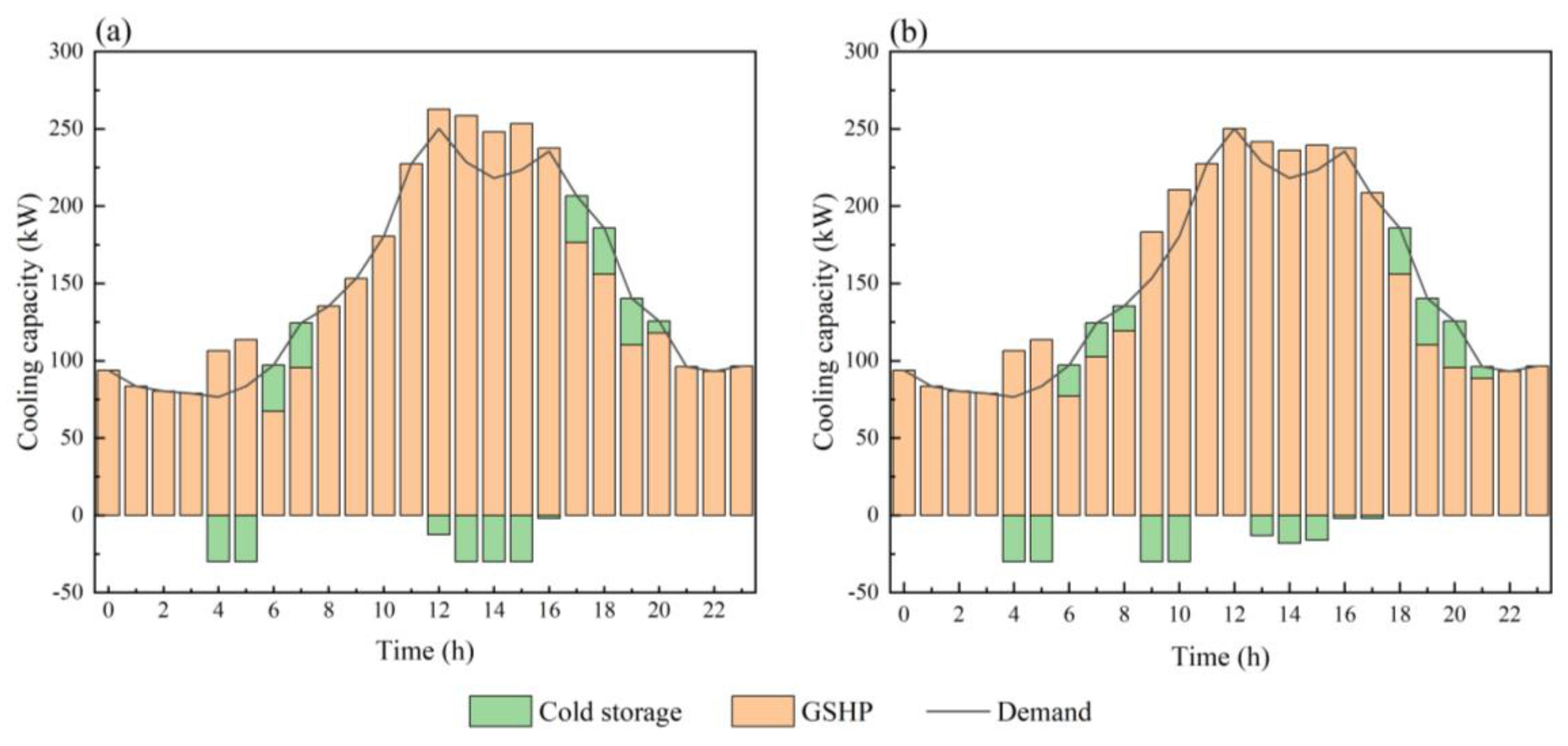
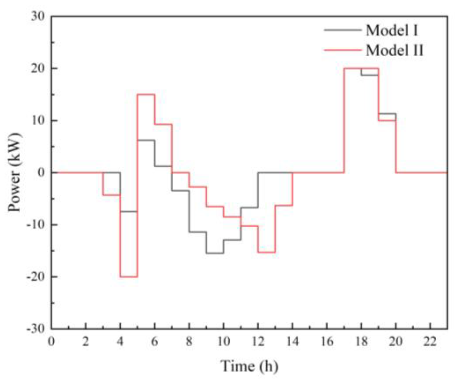
4. Results and Discussion

As shown in Figure 6, when using model II to calculate the pump optimization of the GSHP system operation, the energy consumption of the GSHP unit is greater than that calculated using model I at all times of the day. This is because the COP of the ground source heat pump cannot be maintained at the rated COP all the time during actual operation. The difference in energy consumption calculated by the two models is larger during the periods of 00:00–6:00 and 21:00–24:00, when the load rate is low. During the period of 10:00–19:00, when the load rate is high, the calculated energy consumption of the two types of GSHP units differs by approximately 15%, while during other periods the difference is approximately 30%. This is due to the fact that during operation, the COP of the GSHP unit varies in accordance with the load rate, as illustrated in Figure 3. Subsequently, the COP initially increases and subsequently decreases, attaining its maximum value between 70% and 80% of the load rate.

Optimization of the ground source thermal pump system containing PV storage synergy using the particle swarm algorithm leads to an electrical power balance diagram for the optimal operation strategy, as shown in Figure 7. It is evident that there are three ways to supply energy to the ground source heat pump unit: PV, grid, and storage battery. Before 5:00, the electrical power required by the GSHP system is met solely by the grid. The PV modules produce electricity based on solar irradiation from 6:00 to 19:00, and the energy supply to the GSHP changes during this period. Due to the different energy consumption calculated by model I and model II, the PV power generation exceeds the energy consumption of the GSHP unit at 8:00 and 9:00, respectively. Between 9:00 and 16:00, the PV modules produce electricity, and during this period, the grid needs to meet the energy consumption required for the operation of the ground source heat pump system, in addition to supplying extra electricity to the storage battery. If the storage device is fully used, the system will not be able to fully utilize the PV electricity, resulting in wasted energy. The storage battery releases the stored power during the evening peak tariff hours, thus reducing operating costs.

The cold power balance diagram of the optimal operation strategy calculated by the two models is shown in Figure 8. In the system, the building’s cold demand can be met through the integrated operation of the GSHP unit and cold storage device. It indicated that the operation mode of cold storage devices is mainly influenced by the time-of-use tariff and PV power generation. The cold storage device stores cold during low-tariff periods and releases cold during peak-tariff periods to reduce operating costs. During times of sufficient PV power generation, the operational strategy of the cold storage device will be informed by the specific GSHP model employed.

In calculating the optimal operational strategy, the operation of the energy storage apparatus within the system is prone to change due to the differing operational energy consumption calculated by various GSHP models. Figure 9 depicts the operational diagram of the storage and cooling device, where negative values signify that the storage and cooling device is in a cooling storage state, while positive values indicate that it is in a cooling release state. As illustrated in the figure, the operational state of the cold storage apparatus in models I and II is largely similar. The cold storage device increases the load efficiency of the GSHP during normal periods and releases the cold during peak electricity price hours, thereby effectively lowering the total operational expenditures. The discrepancy in the operation of the cold storage apparatus between the two models is primarily evident during the period between 7:00 and 15:00, which coincides with a surplus of PV power generation relative to the power consumption of the GSHP unit. Consequently, the models necessitate disparate considerations when devising an optimal operational strategy. Given that the COP of the thermal pump unit varies with the load ratio, the cold storage device adopts a strategy of releasing cold from 8:00 to 10:00 by increasing the load rate of the GSHP unit. This approach is employed to enhance the COP of the system, whereas, in model I, no COP variation is observed. The operation of the cold storage unit is guided by two primary considerations: cold loss and time-of-use tariffs.

Figure 10 depicts a relative analysis of the operational characteristics of the batteries within the system. It is evident that there will be a discrepancy between the energy storage battery strategies employed in models I and II, primarily due to the influence of the energy consumption factor. This discrepancy will impact the energy storage batteries, in addition to the difference in operating power. Furthermore, the batteries will exhibit disparate or inverse operating states (e.g., at 3:00, 7:00, and 13:00). If there are multiple power consumers within the system or transferable electrical loads, the choice of model will significantly impact the calculation results.

As evidenced in

Table 3. System optimization results under different models.

	Consumption of Water Pump (kWh)	Consumption of Unit (kWh)	SystemCOP	Operating Costs (CNY)	PV Power Loss Rate
Model I	104	640.42	5.5	114.89	9.5%
Model II	57.41	719.84	4.75	165.90	2.9%

, there is a notable discrepancy in the operational energy consumption of various GSHP models. When calculated using model II, although the pump energy consumption is less than that of model I, the total energy consumption of the GSHP system is greater than model I. Furthermore, the average COP of the GSHP unit is 13.64% smaller. The discrepancy in operational energy expenditure between the two models over the course of a day is 32.16%. Given that photovoltaic (PV) power generation exceeds the consumption of the GSHP in certain periods and that the storage battery is operating at full capacity, the system experiences a PV curtailment at these times. The PV curtailment rate, as calculated using model I, is 9.5%, while the PV curtailment rate of model II is 2.9%. The discrepancy in the calculated rate of PV curtailment can be attributed to the design of the system equipment capacity, the optimal capacity of the storage battery, and the photovoltaic modules utilized. The results of this discrepancy are significant, particularly in light of the varying geothermal heat pump models employed.

5. Conclusions

To illustrate, consider a hotel building in Beijing where an energy system comprising a ground source heat pump is installed. This system serves as the sole source of cooling and heating. Additionally, it incorporates energy storage devices, including cold storage units, batteries, photovoltaic units, power grids, and other functional facilities. An improved particle swarm optimization algorithm is employed with operating cost as the objective function to optimize a system comprising two distinct GSHP models.

It is evident that there is a considerable discrepancy in the operational energy consumption calculated using different GSHP models. The refined model of the GSHP system exhibits greater energy consumption than the simplified model at all times. Furthermore, the calculated energy consumption of the system with refined modeling of the GSHP is consistently higher than that of the system with simplified modeling. The incorporation of soil, buried pipes, and pumps into the model resulted in a notable increase in the total energy consumption of the GSHP system, with an overall rise of 4.4% in the energy consumption of the equipment, including a 12.4% increase in the energy consumption of the heat pump unit decreased by 44.7%, while the average COP of the ground source heat pump system decreased to a value less than the rated COP. This discrepancy is further amplified when the load factor is low or when time-of-day tariffs are modified. Consequently, this gap impacts the operational status of the energy storage device, resulting in a shift in the operational strategy of the energy storage apparatus.

1. The power output of the storage and cooling apparatus fluctuates in each time interval throughout the operational cycle. There is a notable divergence in the operation of the storage and cooling apparatus under the two models during the time interval when sufficient PV power generation is present.

2. The discrepancy in the operational strategy of the storage battery is not merely a contrast in power output; it also encompasses a shift in the initiation and termination of operation within specific time intervals.

The discrepancy in the calculation of energy consumption will result in a divergence in the operational status of the energy storage device. In a system comprising multiple power equipment or a transferable electrical load, the selection of the model will influence the outcome of the calculations. The simplified model’s results for the actual operation of the equipment do not provide meaningful guidance. Moreover, there is a notable discrepancy between the two models regarding the resulting calculations, which markedly influences the preliminary design of the system and its actual operation at a later stage.

References

1. Li, F.; Sun, B.; Zhang, C.; Zhang, L. Operation optimization for combined cooling, heating, and power system with condensation heat recovery. Appl. Energy 2018, 230, 305–316. [Google Scholar] [CrossRef]
2. Chen, K.; Pan, M. Operation optimization of combined cooling, heating, and power superstructure system for satisfying demand fluctuation. Energy 2021, 237, 121599. [Google Scholar] [CrossRef]
3. Li, Q.; Li, Q.; Wang, F.; Wu, J.; Wang, Y. The carrying behavior of water-based fracturing fluid in shale reservoir fractures and molecular dynamics of sand-carrying mechanism. Processes 2024, 12, 2051. [Google Scholar] [CrossRef]
4. Li, L.L.; Liu, Z.F.; Tseng, M.L.; Zheng, S.J.; Lim, M.K. Improved tunicate swarm algorithm: Solving the dynamic economic emission dispatch problems. Appl. Soft Comput. 2021, 108, 107504. [Google Scholar] [CrossRef]
5. De Luca, G.; Ballarini, I.; Lorenzati, A.; Corrado, V. Renovation of a social house into a NZEB: Use of renewable energy sources and economic implications. Renew Energy 2020, 159, 356–370. [Google Scholar] [CrossRef]
6. Park, S.H.; Jang, Y.S.; Kim, E.J. Multi-objective optimization for sizing multi-source renewable energy systems in the community center of a residential apartment complex. Energy Convers. Manag. 2021, 244, 114446. [Google Scholar] [CrossRef]
7. Jo, H.; Park, J.; Kim, I. Environmentally constrained optimal dispatch method for combined cooling, heating, and power systems using two-stage optimization. Energies 2021, 14, 4135. [Google Scholar] [CrossRef]
8. Le, H.T.T.; Sanseverino, E.R.; Nguyen, D.Q.; Di Silvestre, M.L.; Favuzza, S.; Pham, M.H. Critical assessment of feed-in tariffs and solar photovoltaic development in Vietnam. Energies 2022, 15, 556. [Google Scholar] [CrossRef]
9. Yang, C.; Tao, J.; Wuzhi, Z. Source-load coordination economic dispatch method for regional integrated energy system considering wind power accommodation. Power Syst. Technol. 2020, 44, 2474–2483. [Google Scholar]
10. Gao, C.; Zhang, Z.; Wang, P. Day-Ahead Scheduling Strategy Optimization of Electric–Thermal Integrated Energy System to Improve the Proportion of New Energy. Energies 2023, 16, 3781. [Google Scholar] [CrossRef]
11. Yang, Z.P.; Zhang, F.; Liang, J.; Han, X.S.; Xu, Z. Economic generation scheduling of CCHP microgrid with heat pump and energy storage. Power Syst. Technol. 2018, 42, 1735–1743. [Google Scholar]
12. Zhang, Z.L.; Zhang, H.J.; Xie, B.; Zhang, X.T. Energy scheduling optimization of the integrated energy system with ground source heat pumps. J. Clean. Prod. 2022, 365, 132758. [Google Scholar] [CrossRef]
13. Li, B.; Hu, P.; Zhu, N.; Lei, F.; Xing, L. Performance analysis and optimization of a CCHP-GSHP coupling system based on quantum genetic algorithm. Sustain. Cities Soc. 2019, 46, 101408. [Google Scholar] [CrossRef]
14. Zeng, R.; Li, H.; Liu, L.; Zhang, X.; Zhang, G. A novel method based on multi-population genetic algorithm for CCHP–GSHP coupling system optimization. Energy Convers. Manag. 2015, 105, 1138–1148. [Google Scholar] [CrossRef]
15. Ren, J.G.; Zhang, L.; Jin, L.; Tang, Y.; Tang, Q.; Liu, X. Day-ahead economic dispatch model of building integrated energy systems considering the renewable energy consumption. Eng. Sci. Technol. 2023, 55, 160–170. [Google Scholar]
16. Tao, G.; Zhong, W.; Chen, X.; Zhou, G. Low carbon design optimization of integrated energy system with urban thermal power plant as core. Dongnan Daxue Xuebao (Ziran Kexue Ban)/J. Southeast Univ. (Nat. Sci. Ed.) 2022, 52, 631–640. [Google Scholar]
17. Ikeda, S.; Choi, W.; Ooka, R. Optimization method for multiple heat source operation including ground source heat pump considering dynamic variation in ground temperature. Appl. Energy 2017, 193, 466–478. [Google Scholar] [CrossRef]
18. Chen, C.; Chen, X.; Zhang, J.; Yu, K.; Gan, L. Stochastic operational optimal strategy for ground source heat pump system under TOU price. Power Syst. Prot. Control 2019, 47, 57–64. [Google Scholar]
19. Yang, G.; Zhai, X.Q. Optimal design and performance analysis of solar hybrid CCHP system considering influence of building type and climate condition. Energy 2019, 174, 647–663. [Google Scholar] [CrossRef]
20. Guan, X.; Zhang, H.; Xue, C. A method of selecting cold and heat sources for enterprises in an industrial park with combined cooling, heating, and power. J. Clean. Prod. 2018, 190, 608–617. [Google Scholar] [CrossRef]
21. Li, L.L.; Liu, Y.W.; Tseng, M.L.; Lin, G.Q.; Ali, M.H. Reducing environmental pollution and fuel consumption using optimization algorithm to develop combined cooling heating and power system operation strategies. J. Clean. Prod. 2020, 247, 119082. [Google Scholar] [CrossRef]
22. Sanaye, S.; Niroomand, B. Horizontal ground coupled heat pump: Thermal-economic modeling and optimization. Energy Convers. Manag. 2010, 51, 2600–2612. [Google Scholar] [CrossRef]
23. De Ridder, F.; Diehl, M.; Mulder, G.; Desmedt, J.; Van Bael, J. An optimal controlalgorithm for borehole thermal energy storage systems. Energy Build 2011, 43, 2918–2925. [Google Scholar] [CrossRef]
24. Neugebauer, M.; Sołowiej, P. Optimization with the use of genetic algorithms of thelocation depth of horizontal ground heat exchangers. Inżynieria Rol. 2012, 16, 89–97. [Google Scholar]
25. Zeng, H.Y.; Diao, N.R.; Fang, Z.H. A finite line-source model for boreholes in geothermal heat exchangers. Heat Transf. Asian Res. 2002, 31, 558–567. [Google Scholar] [CrossRef]
26. Chen, Y.; Pan, B.; Zhang, X.; Du, C. Thermal response factors for fast parameterized design and long-term performance simulation of vertical GCHP systems. Renew. Energy 2019, 136, 793–804. [Google Scholar] [CrossRef]
27. Soltani, M.; Kashkooli, F.M.; Dehghani-Sanij, A.R.; Kazemi, A.R.; Bordbar, N.; Farshchi, M.J.; Elmi, M.; Gharali, K.; Dusseault, M.B. A comprehensive study of geothermal heating and cooling systems. Sustain. Cities Soc. 2019, 44, 793–818. [Google Scholar] [CrossRef]
28. Hydeman, M.; Gillespie, K.L., Jr. Tools and techniques to calibrate electric chiller component models/discussion. ASHRAE Trans. 2002, 108, 733. [Google Scholar]
29. Wen, Q.; Liu, G.; Wu, W.; Liao, S. Performance evaluation of distributed energy system integrating photovoltaic, ground source heat pump, and natural gas-based CCHP. Energy Convers. Manag. 2022, 252, 115039. [Google Scholar] [CrossRef]
30. Li, X.; Zhang, J.; He, Y.; Zhang, Y.; Liu, Y.; Yan, K. Multi-objective Optimization Dispatching of Microgrid Based on Improved Particle Swarm Algorithm. Electr. Power Sci. Eng. 2021, 37, 1–7. [Google Scholar]
31. Fu, X.; Huang, S.; Li, R.; Sun, H. Electric power output optimization for CCHP using PSO theory. Energy Procedia 2016, 103, 9–14. [Google Scholar] [CrossRef]
32. Tharwat, A.; Elhoseny, M.; Hassanien, A.E.; Gabel, T.; Kumar, A. Intelligent Bézier curve-based path planning model using Chaotic Particle Swarm Optimization algorithm. Clust. Comput. 2019, 22, 4745–4766. [Google Scholar] [CrossRef]
33. Zhang, B.; You, S.; Wang, S.; Ding, X.; Wang, C.; Gao, Y. From laboratory to on-site operation: Reevaluation of empirically based electric water chiller models. Build. Simul. 2022, 15, 213–232. [Google Scholar] [CrossRef]
Figure 1. System energy structure.
Energies 17 06023 g001
Figure 2. Comparison of outlet temperature results of buried pipes.
Energies 17 06023 g002
Figure 3. Performance of heat pump unit under partial load.
Energies 17 06023 g003
Figure 4. Building demand, PV power generation and outdoor temperature.
Energies 17 06023 g004
Figure 5. Flow chart of improved PSO algorithm.
Energies 17 06023 g005
Figure 6. GSHP system energy consumption and price of electricity.
Energies 17 06023 g006
Figure 7. Electrical power balance diagram of the system, (a) is model I, (b) is model II.
Energies 17 06023 g007
Figure 8. Cold power balance diagram of the system, (a) model I, (b) model II.
Energies 17 06023 g008
Figure 9. Operation diagram of cold storage device.
Energies 17 06023 g009
Figure 10. Operation diagram of power storage device.
Energies 17 06023 g010