Co-Optimization of Speed Planning and Energy Management for Plug-In Hybrid Electric Trucks Passing Through Traffic Light Intersections

Abstract

To tackle the energy-saving optimization issue of plug-in hybrid electric trucks traversing multiple traffic light intersections continuously, this paper presents a double-layer energy management strategy that utilizes the dynamic programming–twin delayed deep deterministic policy gradient (DP-TD3) algorithm to synergistically optimize the speed planning and energy management of plug-in hybrid electric trucks, thereby enhancing the vehicle’s passability through traffic light intersections and fuel economy. In the upper layer, the dynamic programming (DP) algorithm is employed to create a speed-planning model. This model effectively converts the nonlinear constraints related to the position, phase, and timing information of each traffic signal on the road into time-varying constraints, thereby improving computational efficiency. In the lower layer, an energy management model is constructed using the twin delayed deep deterministic policy gradient (TD3) algorithm to achieve optimal allocation of demanded power through the interaction of the TD3 agent with the truck environment. The model’s validity is confirmed through testing on a hardware-in-the-loop test machine, followed by simulation experiments. The results demonstrate that the DP-TD3 method proposed in this paper effectively enhances fuel economy, achieving an average fuel saving of 14.61% compared to the dynamic programming–charge depletion/charge sustenance (DP-CD/CS) method.

1. Introduction

As the global economy advances and urbanization accelerates, the widespread reliance on traditional internal combustion locomotives has resulted in a rise in carbon dioxide emissions and other pollutants [1]. According to statistics, greenhouse gas emissions from the transportation industry account for 28% of total greenhouse gas emissions [2]. In 2020, China unveiled its explicit commitment to reach carbon peak by 2030 and achieve carbon neutrality by 2060. The “dual-carbon” strategy advocates for embracing a green, environmentally friendly, and low-carbon lifestyle; fostering robust growth in renewable energy; and actively advancing energy restructuring. Improving fuel efficiency and reducing carbon emissions have become urgent issues to address due to the low fuel utilization of traditional internal combustion locomotives [3,4]. At present, with the development of science and technology, the research on energy saving of vehicles has a new development direction. Connected vehicles improve vehicle safety and economy by sensing traffic information and integrating it with the vehicle power system [5,6]. This approach, which optimizes driving speed by sensing environmental information to achieve energy conservation and emission reduction, is termed eco-driving [7]. Hence, merging eco-driving optimization with hybrid electric vehicle energy management can significantly enhance the fuel efficiency of such vehicles.

According to the road conditions and traffic light conditions provided by the driving scenario of the connected vehicle, the speed planning of eco-driving is mainly divided into two planning methods: without considering traffic lights and considering traffic lights [8]. Speed planning without considering traffic lights is a low-dimensional optimization problem, which is beneficial to reducing computational burden and has attracted the attention of many researchers. Sanker et al. [9] utilized a vector autoregressive model to forecast the speed of the leading vehicle and subsequently optimized the vehicle’s speed using these forecasted data. The energy efficiency of this method was improved by 19% compared to human drivers. Huang et al. [10] employed a genetic algorithm to optimize the global speed profile, followed by local speed adaptation using the interior point method, leading to a notable reduction in fuel consumption. Pan et al. [11] constructed a layered eco-driving strategy. The upper layer employs a genetic algorithm for vehicle speed planning. The lower layer utilizes synovial control to maintain a safe distance between the vehicle and the one in front. This method reduces the average energy consumption of the fleet by 24% compared to adaptive cruise control. These eco-driving methods, which do not take into account the effects of traffic signals, are targeted at specific driving scenarios with multiple vehicles, and all contribute to the overall energy efficiency of the fleet.

For single vehicle driving scenarios, complex constraints, such as traffic signals and road speed limits, are usually considered for speed planning [12]. Sun et al. [13] used a data-driven approach to formulate chance constraints to turn red-light duration into a random variable and then solved this optimization problem using dynamic programming, which significantly improved the efficiency of vehicles passing through intersections with uncertain traffic signal timings. Guo et al. [14] introduced an innovative real-time energy management approach for fuel cell hybrid electric buses in their study. This method is aimed at prolonging the service life of the fuel cell engine by strategically adjusting speeds at intersections to minimize load fluctuations during vehicle travel. Wei et al. [15] introduced a dual dynamic programming-based speed-planning approach and applied a modified alternating direction method of multipliers (ADMM) algorithm to optimize fuel cell system power. Their aim was to achieve synergistic optimization of speed planning and energy management for vehicles traversing signalized intersections.

Energy management strategies for hybrid electric vehicles typically fall into two categories: rule-based control strategies and optimization-based control strategies [16]. Rule-based energy management strategies mainly include fuzzy logic control strategies [17], state machine control strategies [18], charge depleting–charge sustaining control strategies, etc. The rule-based control strategy, grounded in engineering expertise and mathematical models, is a fundamental approach to energy management. It has strong robustness and is widely used in practice, but it cannot achieve optimal control results [19]. The optimization-based energy management strategy aims to minimize the objective function while satisfying vehicle dynamics constraints, thereby reducing the overall vehicle operational costs [20]. Optimization-based energy management strategies typically classify into global and instantaneous optimization strategies [21]. For global optimization strategies, the most typical is the dynamic programming (DP) control strategy [22]. The DP control strategy is optimized based on the whole driving cycle, which can guarantee the global optimum and is usually used as a benchmark for other control strategies [23]. Gissing et al. [24] proposed a hybrid optimization method combining dynamic programming with genetic algorithms which greatly improves the fuel-saving potential of the vehicle, and the fuel savings can be up to 40% compared to charge depletion–charge sustenance (CDCS). Peng et al. [25] investigated the Pontryagin minimum principle (PMP) energy management strategy that considers the dynamic limitation of fuel cell power, which reduces the dynamic oscillations during fuel cell operation and improves the fuel economy. However, since the PMP control strategy requires prior knowledge of global driving conditions, its application is limited to offline scenarios. For transient optimization strategies, the most typical is the model predictive control (MPC) strategy. Xiang et al. [26] developed an adaptive Markov chain-based MPC energy management strategy, which relies on real-time vehicle load prediction through Markov chain analysis. This approach enhances both the real-time performance and fuel economy of the energy management strategy. Xu et al. [27] proposed a model predictive control strategy based on real-time traffic information. The control strategy constructed a traffic density model using a chained Gaussian process approach, which transformed the traffic information prediction problem into a dynamically constrained nonlinear optimal control problem, further improving the economy of the energy management strategy. These optimization-based energy management strategies enhance hybrid electric vehicle fuel economy. Nonetheless, while global optimization strategies lack real-time applicability, instantaneous optimization strategies may not ensure global optimality. Therefore, these traditional optimization-based energy management strategies have conflicts between real-time performance and global optimality [28].

In addition to traditional optimization methods, reinforcement learning methods have also been applied to the energy management strategies of vehicles, effectively balancing the real-time and optimal properties of the strategy [29]. Reinforcement learning methods are used to achieve autonomous learning through interaction with the environment and to make decisions about the objects under control [30]. Q-learning is a foundational approach within reinforcement learning. Xiong et al. [31] introduced an energy management method for plug-in hybrid electric vehicles based on Q-learning. The method further optimizes the computational efficiency of the system by determining the update of the strategy through the Kullback–Leibler (KL) scatter rate and discusses the effect of circumstances such as temperatures, states of health, SOC, and driving cycles on the control strategy. Q-learning saves states and actions by building a Q-table; however, as the dimensions of states and actions increase, it makes the Q-table dimensions larger and larger, thus making it impossible to achieve a fast solution [32]. Subsequently, the deep Q-learning (DQL) method was developed, replacing Q-tables with deep neural networks, offering a viable solution to handle high-dimensional states and actions. Qi et al. [33] devised an energy management strategy for plug-in hybrid electric vehicles using deep reinforcement learning. Both the deep Q-network (DQN) method and the dueling deep Q-network (DDQN) method proved effective in enhancing vehicle fuel efficiency. However, DDQN exhibited faster convergence compared to DQN during training.

At present, artificial intelligence methods such as deep reinforcement learning are being effectively applied in hybrid electric vehicle energy management strategies. These methods have strong learning abilities and adaptability, enabling them to cope with complex driving conditions. To further improve fuel economy, many scholars have conducted in-depth studies on eco-driving, which enhances fuel efficiency by changing driving behaviors. However, existing studies mainly focus on scenarios without traffic lights, and there are fewer studies on eco-driving for hybrid electric vehicles in the presence of traffic signals. Optimizing vehicle trajectories in urban traffic environments has great potential for energy savings. Deep reinforcement learning-based methods not only show potential for real-time applications but also improve the accuracy and stability of algorithms through extensive training. Therefore, introducing artificial intelligence algorithms such as deep reinforcement learning into eco-driving and energy management for collaborative optimization is highly meaningful.

In this paper, a two-layer energy management strategy based on the DP-TD3 algorithm is proposed to improve the fuel economy of hybrid electric trucks. In the upper layer, a dynamic programming (DP) algorithm is used to determine the optimal speed for a vehicle passing through multiple traffic light intersections. In the lower layer, a twin delayed deep deterministic policy gradient (TD3) algorithm is used to determine the optimal power allocation between the engine and the electric motor of the plug-in hybrid electric truck. The main contributions of this study are as follows: (1) A double-layer energy management strategy for DP-TD3 is proposed. The speed planning and energy management of a plug-in hybrid electric truck are co-optimized to improve the vehicle’s fuel economy and passability at traffic signal intersections. (2) A speed-planning model based on the DP algorithm is constructed, which improves computational efficiency by transforming the nonlinear constraints of traffic signals into time-varying constraints. (3) Simulation experiment results show that the DP-TD3 method achieves an average fuel saving of 14.61% compared to the DP-CD/CS method.

2. Plug-In Hybrid Electric Truck System Modeling

This section primarily introduces the physical model of plug-in hybrid electric trucks and the traffic signal model of the external environment. It covers the truck’s structure, longitudinal dynamics model, engine model, motor model, battery model, and traffic signal model. We assume that the truck operates without interference from other vehicles on the road, lateral motion of the vehicle is neglected, and there is no communication delay between the truck and the traffic signals.

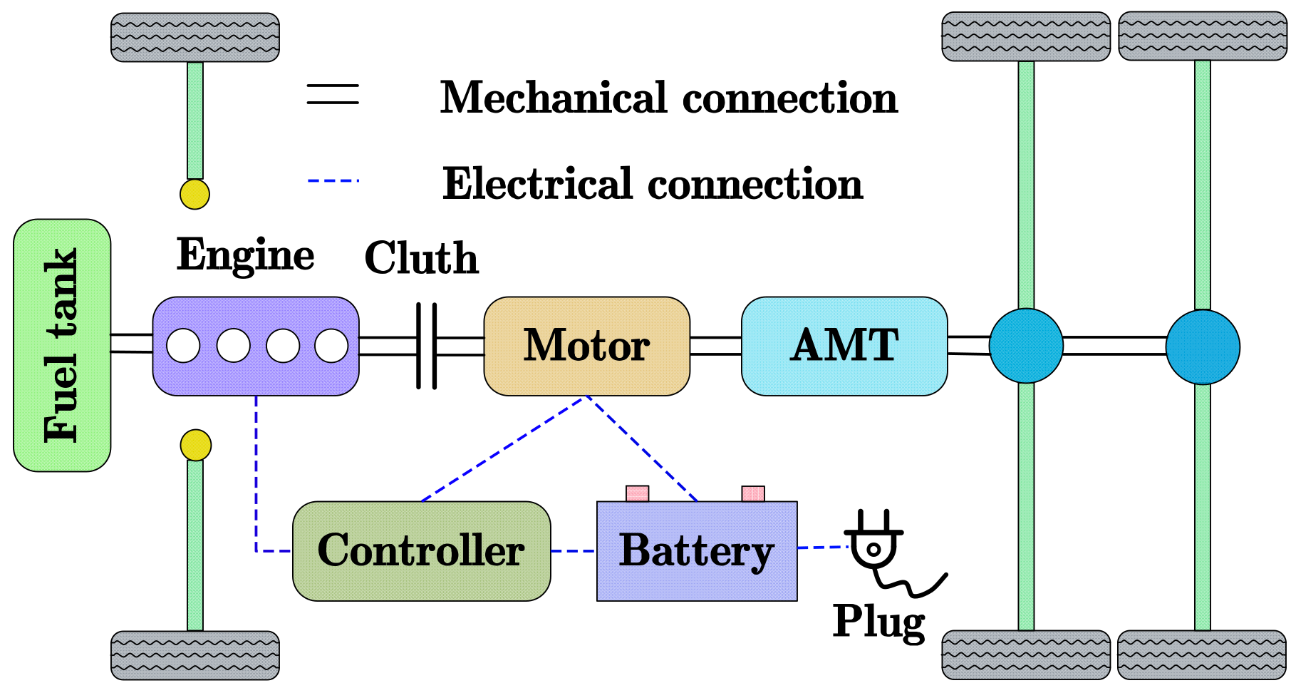
2.1. Plug-In Hybrid Electric Truck System

This study focuses on the Chenglong truck manufactured by Dongfeng Liuzhou Motor Co., Ltd. (Liuzhou, China), a single-axle parallel plug-in hybrid electric truck. The powertrain of this truck primarily consists of an engine, an electric motor, a clutch, a controller, and an automatic transmission. The engine is equipped with a starter, which allows it to be promptly started to provide power to the vehicle. The electric motor can function as both a power source for driving the vehicle and a generator for recovering braking energy. The battery mainly supplies power to the motor. The clutch facilitates the vehicle’s operation in motor-driven mode, engine-driven mode, hybrid-driven mode, and regenerative braking mode through its engagement and disengagement with the engine. These different operating modes contribute to further improving the fuel economy of the plug-in hybrid electric truck. The structure of the plug-in hybrid electric truck is shown in Figure 1, and the main characteristic parameters of the PHET are listed in

Table 1. The main characteristic parameters of PHET.

Component	Parameters	Values
Vehicle	Gross vehicle weight	18,000 kg
	Frontal area	5.1 m2
	Coefficient of air resistance	0.527
	Motor transmission ratio	5.48
	Automatic mechanical transmission	10.36, 6.48, 4.32, 3.47, 2.4, 1.5, 1, 0.8
	Final drive ratio	3.909
Motor	Maximum power	158.3 kw
	Maximum torque	293 Nm
	Maximum speed	12,000 r/min
Engine	Maximum power	169.1 kw
	Maximum torque	734 Nm
	Rated speed	2200 r/min
Battery	Rated voltage	560.28 V
	Capacity	5 Ah
	Rated power	78.4 kw

.

2.2. Vehicle Longitudinal Dynamics Model

According to the longitudinal dynamics analysis of the vehicle, the driving resistance of the plug-in hybrid electric truck is expressed as follows [16]:

$$\left\{\begin{array}{l}{F}_t=F_f+F_w+F_i+F_j\hfill \\ F_f=mgf\cos \alpha \\ F_w={\displaystyle \frac{1}{2}}{C}_{D}A\rho u_a^2\\ F_i=mg\sin \alpha \\ F_j=\delta m{\displaystyle \frac{du}{dt}}\end{array}\right.$$

(1)

where $F_f$ is rolling resistance, $F_w$ is air resistance, $F_i$ is gradient resistance, $F_j$ is acceleration resistance, $m$ is vehicle mass, $g$ is gravitational acceleration, $f$ is rolling resistance coefficient, $\alpha$ is road gradient, $C_D$ is air resistance coefficient, $A$ is the windward area, $\rho$ is the air density, $u_a$ is the vehicle speed, $\delta$ is the rotational mass conversion coefficient, and ${\displaystyle \frac{du}{dt}}$ is the acceleration of the vehicle.

The demanded power of the vehicle is as follows:

$$P_{dem}=\frac{1}{\eta }\left(F_f+F_w+F_i+F_j\right)u_a$$

(2)

where $\eta$ is the mechanical transmission efficiency.

Plug-in hybrid electric trucks are powered by an engine and a motor, represented by the following equation:

$$P_{dem}=\left(P_{eng}+P_{mot}\right)\eta$$

(3)

where $P_{eng}$ is the engine power, and $P_{mot}$ is the motor power.

2.3. Powertrain Component Model

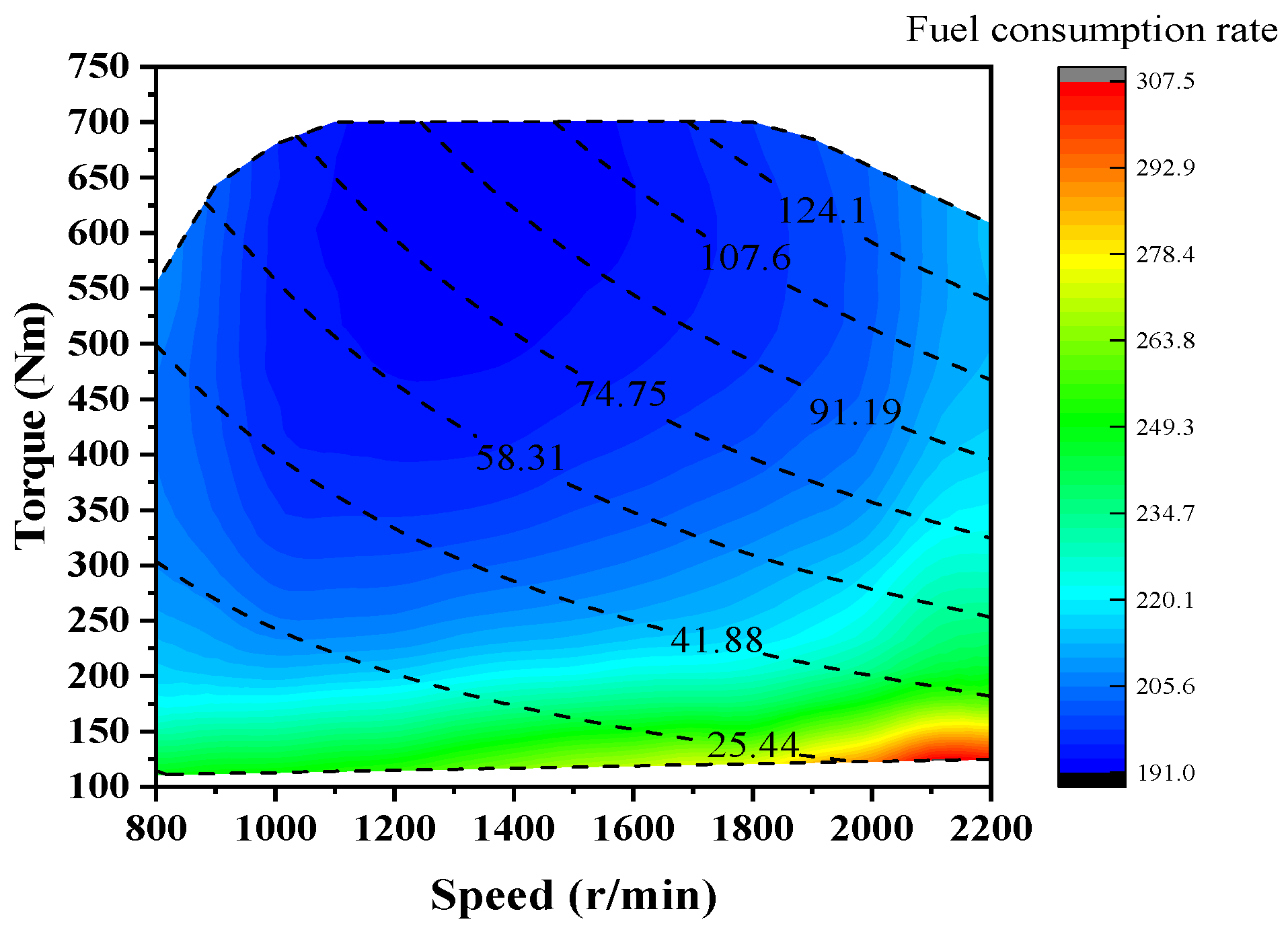
2.3.1. Engine Model

In this paper, the engine is modeled in a quasi-static form, disregarding the influences of environmental changes and other operational factors affecting the engine [34]. The engine’s fuel consumption rate data were obtained through bench tests and provided by Dongfeng Liuzhou Motor Co., Ltd. Its fuel consumption rate map is shown in Figure 2. We performed two-dimensional linear interpolation on the fuel consumption map (Figure 2) to calculate the engine’s fuel consumption rate. Therefore, the relationship between the engine’s fuel consumption rate, rotational speed, and torque can be expressed as follows:

$$b_{eng}=f\left(n_{eng},T_{eng}\right)$$

(4)

where $b_{eng}$ is the fuel consumption rate of the engine, $n_{eng}$ is the speed of the engine, and $T_{eng}$ is the torque of the engine.

2.3.2. Motor Model

The motor is modeled using a numerical approach [35], with data provided by Dongfeng Liuzhou Motor Co., Ltd. The motor efficiency map is shown in Figure 3. We performed two-dimensional linear interpolation on the motor efficiency map (Figure 3) to calculate the motor efficiency. Therefore, the motor power can be expressed as follows:

$$\left\{\begin{array}{l}{P}_{mot}=2\pi T_{mot}{n}_{mot}{\eta }_{mot}/60\hfill \\ {\eta }_{mot}=f\left(n_{mot},T_{mot}\right)\hfill \end{array}\right.$$

(5)

where $P_{mot}$ is the motor power, $T_{mot}$ is the motor torque, $n_{mot}$ is the motor speed, and ${\eta }_{mot}$ is the motor efficiency.

2.3.3. Battery Model

The battery employs an equivalent internal resistance model. The current expression for the battery is as follows:

$$I\left(t\right)={\displaystyle \frac{U_0-\sqrt{U_0^2-4R_0{P}_b}}{2R_0}}$$

(6)

where $I\left(t\right)$ is the current of the battery, $U_0$ is the open circuit voltage, $R_0$ is the battery internal resistance, and $P_b$ is the power of the battery.

The expression for the state of charge of the battery can be denoted as follows:

$$SOC\left(t\right)=SO{C}_0-{\displaystyle \frac{{\displaystyle {\int }_0^{t}I\left(t\right)}dt}{Q_b}}$$

(7)

where $SOC\left(t\right)$ is the SOC of the battery, $SO{C}_0$ is the initial state SOC of the battery, and $Q_b$ is the capacity of the battery.

2.4. Traffic Signal Light Model

When a vehicle approaches a traffic signal, it must stop and wait if the signal is red, but it can proceed if the signal is green. The schematic diagram of the vehicle passing through a traffic signal is shown in Figure 4. In the diagram, $t_r$ represents the red light duration, $t_g$ represents the green light duration, $t_1$ represents the time required to pass through the traffic signal, and $t_2$ represents the time during which the signal is green while passing through the traffic signal. Therefore, the vehicle must pass within the $t_2$ time period to avoid stopping at the traffic signal. Suppose there are N traffic signals on a road of length S, where the location of the kth traffic signal is $S^k\in \left[0,s_d\right]$, $k\in \left\{1,2,3,\dots ,N\right\}$. The cycle time, $t_l^k$, relative to the absolute driving time, t, is as follows:

$$t_l^k=mod\left(t_{l0}^k+t,T^k\right)$$

(8)

$$T^k=T_g^k+T_r^k$$

(9)

where $t_{l0}^k\in \left[0,T^k\right]$ is the initial value of $t_l^k$, $T^k$ is the cycle period of the kth signal light, $T_g^k$ is the green light duration of the kth signal light, and $T_r^k$ is the red light duration of the kth signal light.

3. Energy Management Strategy Based on Dynamic Programming–Twin Delayed Deep Deterministic Policy Gradient Algorithm

3.1. Energy Management Strategy Framework

The hierarchical energy management strategy framework based on the DP-TD3 algorithm proposed in this study is illustrated in Figure 5. This control strategy is divided into two hierarchical levels. The upper level comprises a speed-planning model based on the DP algorithm, as shown in the solid-line box at the top of Figure 5. Its functions are as follows: The DP algorithm is employed to plan the speed of vehicles passing through multiple traffic light intersections and to determine the optimal vehicle speed for passing traffic lights. This approach aims to avoid the need to stop at red lights during operation, thereby maximizing fuel consumption reduction. Traffic light information along the route is obtained in advance via V2X technology. When performing speed planning, the nonlinear constraints of traffic signals are transformed into time-varying constraints, thus reducing the model’s complexity and accelerating computation. The lower layer is an energy management model based on the TD3 algorithm, as shown in the dashed line box at the bottom of Figure 5. Its functions are as follows: The energy management model manages the vehicle’s power sources based on the speed planned by the upper-layer strategy, further improving the fuel economy of hybrid trucks. The energy management strategy, formulated using the TD3 algorithm, leverages the advantages of reinforcement learning, enabling the agent to interact with the environment in real time to optimize energy distribution. The core structure of the TD3 algorithm is the actor–critic architecture, which uses two Q-value networks (critics) and one actor network to learn and optimize the policy. This structure effectively enhances the stability and efficiency of policy learning. The first dashed box at the bottom of Figure 5 represents the agent component of the TD3 algorithm, while the second dashed box represents the environment component, which corresponds to the plug-in hybrid truck model constructed in Section 2 of this study.

3.2. Upper-Level Speed-Planning Control

3.2.1. Speed-Planning Model

In the construction of the speed-planning model, this paper only considers the longitudinal speed of vehicles and assumes that the location of traffic lights and signal phasing and timing can be obtained in time through Vehicle-to-Infrastructure (V2I). The truck’s speed is planned according to the timing of traffic light signals to minimize the vehicle’s waiting time at intersections, thereby reducing energy consumption. Consequently, the cost function of the vehicle speed-planning model is defined as follows:

$$J_h={\displaystyle {\int }_0^{s_d}\frac{{\dot{m}}_{fuel}}{v\left(s\right)}}ds$$

(10)

The kinematic model of the vehicle is as follows:

$$\frac{d}{ds}\left(\begin{array}{c}t\\ v\end{array}\right)=\frac{1}{v\left(s\right)}\left(\begin{array}{c}1\\ \dot{v}\end{array}\right)$$

(11)

To enhance computational efficiency, the vehicle’s speed-planning energy consumption model is simplified as follows:

$$J_h={\displaystyle {\int }_0^{s_d}}\frac{P_w(v,a)}{v\left(s\right)}ds$$

(12)

$$P_w=\frac{1}{2}\rho C_{D}A{v}^3+mgfv+mav$$

(13)

where $P_w$ is the current vehicle driving power, $\rho$ is the air density, $C_D$ is the wind resistance coefficient, $A$ is the windward area, $f$ is the rolling resistance coefficient, and $g$ is the gravitational acceleration.

In this paper, the limiting reference trajectory of a vehicle passing through a traffic signal is constructed by transforming the nonlinear constraints of the signal into time-varying constraints. The upper reference trajectory is determined from the green window of the traffic signal. The lower reference trajectory is determined based on the end of the green light window through which the vehicle passes. The upper and lower reference trajectories of the vehicle are shown in Figure 6, where the red line segments indicate the positions of red traffic lights. The upper and lower reference trajectories represent the boundary limits for the vehicle passing through the traffic lights, ensuring the vehicle travels between the two trajectories. The acceleration model for the upper reference trajectory is as follows:

$$a_h=\left\{\begin{array}{cc}{a}_{\max }\left[1-{\left(\frac{v}{v_{\max }}\right)}^4-{\left(\frac{s^{*}\left(v,\Delta v\right)}{\Delta x}\right)}^2\right]& \mathrm{green} \mathrm{traffic} \mathrm{light}\\ -\frac{v^2}{2\Delta x}& \mathrm{red} \mathrm{traffic} \mathrm{light}\end{array}\right.$$

(14)

$$s^{*}\left(v,\Delta v\right)=s_0+\max \left[0,v{t}_g+\frac{v\Delta v}{2\sqrt{a_{\max }b}}\right]$$

(15)

where $s^{*}\left(v,\Delta v\right)$ is the desired distance, $\Delta v$ is the velocity step, $\Delta x$ is the distance step, $t_g$ is the desired time interval, and $b$ is the maximum deceleration of the vehicle.

The time-varying constraints that should be satisfied by the driving distance of the vehicle are as follows:

$$s_l\left(t\right)\le s\left(t\right)\le s_h\left(t\right)$$

(16)

where $s_l\left(t\right)$ is the lower reference trajectory, and $s_h\left(t\right)$ is the upper reference trajectory.

The corresponding time constraint is as follows:

$$t_l\left(s\right)\le t\left(s\right)\le t_h\left(s\right)$$

(17)

where $t_l\left(s\right)$ is the time corresponding to $s_l\left(t\right)$, and $t_h\left(s\right)$ is the time corresponding to $s_h\left(t\right)$.

The final driving time of a vehicle can be simplified as follows:

$$t_d=\left(t_l\left(s_d\right)+t_h\left(s_d\right)\right)/2$$

(18)

3.2.2. Speed-Planning Control Strategy Based on Dynamic Programming (DP) Algorithm

The dynamic programming algorithm is a mathematical optimization method used to solve multi-stage decision optimization problems. Its primary concept involves transforming a multi-stage problem into a single-stage problem and utilizing the optimal solution of the single stage to determine the global optimal solution. In this paper, a dynamic planning algorithm is used to plan the speed of vehicles through traffic signals, thus avoiding the vehicle stopping due to encountering a red light when passing through a traffic signalized intersection. The control strategy has vehicle acceleration, $a$, as the control variable, and time ($t$) and velocity (v) as the state variables. The speed-planning problem based on the DP algorithm can be expressed as follows:

$$\begin{gathered} \min J_h={\displaystyle {\int }_0^{s_d}}\frac{P_w(v,a)}{v\left(s\right)}ds={\displaystyle {\int }_0^{t_d}m\left(av+gfv+\frac{\rho C_{D}A\overline{v}}{2m}{v}^2\right)}dt \\ \frac{d}{ds}\left(\begin{array}{c}t\\ v\end{array}\right)=\frac{1}{v\left(s\right)}\left(\begin{array}{c}1\\ \dot{v}\end{array}\right) \\ t\left(0\right)=0,v\left(0\right)=v_0,\overline{v}=s_d/t_d \\ {t}_{\min }\le t\left(s\right)\le t_{\max } \\ {v}_{min}\le v\left(s\right)\le v_{\max } \\ {a}_{\min }\le a\left(s\right)\le a_{\max } \end{gathered}$$

(19)

3.3. Lower-Level Energy Management Control

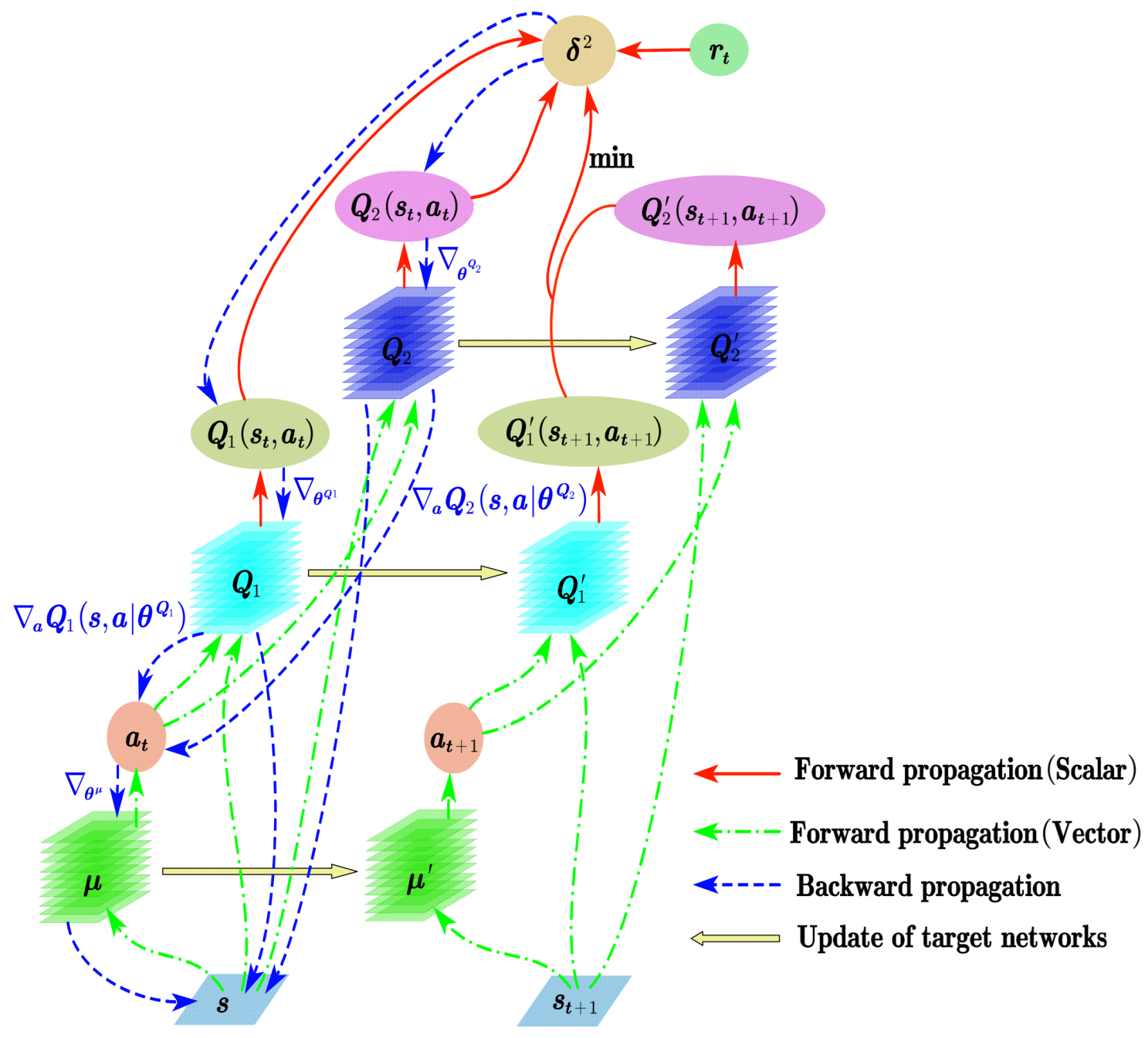
3.3.1. Twin Delayed Deep Deterministic Policy Gradient (TD3) Algorithm

Deep reinforcement learning primarily achieves action strategy optimization through the interaction between the agent and the environment, and it has found widespread applications in optimization engineering design. The twin delayed deep deterministic policy gradient (TD3) algorithm is an optimization of the deep deterministic policy gradient (DDPG) algorithm, addressing the issue of Q-value overestimation in traditional deep learning algorithms. The network structure of TD3 is illustrated in Figure 7, and the pseudo-code is presented in Algorithm 1.

Algorithm 1: TD3

Initialize critic networks, $Q_1$ and $Q_2$, and actor network, $\mu$, with parameters ${\theta }^{Q_1}$, ${\theta }^{Q_2}$, and ${\theta }^{\mu }$  Initialize target, networks ${\theta }^{Q_1^{\prime }}\leftarrow {\theta }^{Q_1}$, ${\theta }^{Q_2^{\prime }}\leftarrow {\theta }^{Q_2}$, ${\theta }^{{\mu }^{\prime }}\leftarrow {\theta }^{\mu }$  Initialize replay buffer, $\mathrm{D}$  Initialize learning rate, $\tau$  for t = 1:T do   Initialize a random noise, $\mathcal{N}\left(0,{\sigma }^2\right)$   Initialize state variables, ${\mathrm{s}}_t=[\mathrm{v},{\mathrm{a}}_c,\mathrm{S}\mathrm{O}\mathrm{C}]$   According to states, ${\mathrm{s}}_t$, selection action, ${\mathrm{a}}_t=\mu \left({\mathrm{s}}_t|{\theta }^{\mu }\right)+\mathcal{N}$   Get reward $\mathrm{r}$ and new state ${\mathrm{s}}_{t+1}$   Store transition tuple $({\mathrm{s}}_t,{\mathrm{a}}_t,\mathrm{r},{\mathrm{s}}_{t+1})$ in replay buffer, $\mathrm{D}$   Randomly sample mini batch of N transitions $({\mathrm{s}}_t,{\mathrm{a}}_t,\mathrm{r},{\mathrm{s}}_{t+1})$ from $\mathrm{D}$   $\widehat{\mathrm{a}}\leftarrow {\mu }^{\prime }\left(s_{t+1}|{\theta }^{{\mu }^{\prime }}\right)+\zeta$, $\zeta ~\mathrm{c}\mathrm{l}\mathrm{i}\mathrm{p}(\mathcal{N}\left(0,{\sigma }^2\right),-\mathrm{c},\mathrm{c})$   $\mathrm{y}\leftarrow \mathrm{r}+\gamma \mathrm{m}\mathrm{i}{\mathrm{n}}_{i=\mathrm{1,2}}{\mathrm{Q}}_i^{\prime }(s_{t+1},{\widehat{a}}_t|{\theta }^{Q_i^{\prime }})$   Update critic network parameters  ${\theta }^{Q_i}\leftarrow argmi{n}_{{\theta }^{Q_i}}{N}^{-1}\sum (y-Q_i(s_t,a_t\left|{\theta }^{Q_i}\right){)}^2$   if t mod d, then    Update $\mu$ by the deterministic policy gradient  ${\nabla }_{{\theta }^{\mu }}J\left({\theta }^{\mu }\right)=E\left[{\nabla }_a{Q}_1\right(s_t,a_t\left|{\theta }^{Q_1}\right){\nabla }_{{\theta }^{\mu }}\mu \left(s_t\right|{\theta }^{\mu }\left)\right]$    Update target network parameters  ${\theta }^{Q_i^{\prime }}\leftarrow \tau {\theta }^{Q_i}+(1-\tau ){\theta }^{Q_i^{\prime }}$  ${\theta }^{{\mu }^{\prime }}\leftarrow \tau {\theta }^{\mu }+(1-\tau ){\theta }^{{\mu }^{\prime }}$    end if   end for

The TD3 algorithm [36] comprises two typical neural networks; the actor network, $\mu$; and the critic network, Q. The parameter of the actor network µ is ${\theta }^{\mu }$, and the parameter of the critical network Q is ${\theta }^Q$. The actor network evaluates the input state, s, and provides an action, a, while the critic network evaluates both the inputs and outputs of the actor network, updating its network parameters accordingly in real time. The critical network contains two of them, $Q_1(s,a|{\theta }^{Q_1})$ and $Q_2(s,a|{\theta }^{Q_2})$, and its corresponding target networks are $Q_1^{\prime }(s,a|{\theta }^{Q_1})$ and $Q_2^{\prime }(s,a|{\theta }^{Q_2})$. TD3 addresses the issue of overestimated Q-values by selecting the minimum output value from two target critic networks to compute the target Q-value. The actor network corresponds to the target network as ${\mu }^{\prime }$. To enhance policy stability, the actor network and target network are not updated synchronously with the critic network. Instead, they are updated only when the critic network reaches a predetermined number of steps.

The TD3 algorithm uses Temporal Difference (TD) to update the Q-value estimates. The TD error can be expressed as follows:

$$y_{target}\left(t\right)=r\left(s_t,a_t\right)+\gamma \underset{i=1,2}{\min }{Q}_i^{\prime }(s_{t+1},{\widehat{a}}_{t+1}|{\theta }^{Q_i^{\prime }})$$

(20)

$$\delta \left(t\right)=y_{target}\left(t\right)-Q_i\left(s_t,a_t|{\theta }^{Q_i}\right)$$

(21)

where $y_{target}\left(t\right)$ is the target network Q, $r$ is the reward function, and $\gamma$ is the discount factor for reward.

The loss function and gradient of the critic network are as follows:

$$L\left({\theta }^{Q_i}\right)=E\left[{\left(y_{target}\left(t\right)-Q_i\left(s_t,a_t|{\theta }^{Q_i}\right)\right)}^2\right]$$

(22)

$${\nabla }_{{\theta }^{Q_i}}L\left({\theta }^{Q_i}\right)=E\left[\left(y_{target}-Q_i\left(s_t,a_t|{\theta }^{Q_i}\right)\right){\nabla }_{{\theta }^{Q_i}}{Q}_i\left(s_t,a_t|{\theta }^{Q_i}\right)\right]$$

(23)

The parameters, ${\theta }^{\mu }$, are updated by training the actor network to maximize the cumulative reward. The objective function and gradient of the actor network can be expressed as follows:

$$J\left({\theta }^{\mu }\right)=E\left[Q_1\left(s_t,\mu \left(s_t\right)\right)\right]$$

(24)

$${\nabla }_{{\theta }^{\mu }}J\left({\theta }^{\mu }\right)=E\left[{\nabla }_a{Q}_1\left(s_t,a_t|{\theta }^{Q_1}\right){\nabla }_{{\theta }^{\mu }}\mu \left(s_t|{\theta }^{\mu }\right)\right]$$

(25)

The update formula for the critic network can be described as follows:

$${\theta }^{Q_i}\leftarrow {\theta }^{Q_i}+\alpha \cdot {\nabla }_{{\theta }^{Q_i}}L\left({\theta }^{Q_i}\right)$$

(26)

where $\alpha$ is the learning rate of the critic network.

The update formula for the actor network is represented as follows:

$${\theta }^{\mu }\leftarrow {\theta }^{\mu }+\beta \cdot {\nabla }_{{\theta }^{\mu }}J\left({\theta }^{\mu }\right)$$

(27)

where $\beta$ is the learning rate of the actor network.

The update formula for the corresponding target network of the critic network is as follows:

$${\theta }^{Q_i^{\prime }}\leftarrow \tau {\theta }^{Q_i^{\prime }}+\left(1-\tau \right){\theta }^{Q_i^{\prime }}$$

(28)

where τ is the soft update rate factor.

The update formula for the corresponding target network of the actor network can be represented as follows:

$${\theta }^{{\mu }^{\prime }}\leftarrow \tau {\theta }^{\mu }+\left(1-\tau \right){\theta }^{{\mu }^{\prime }}$$

(29)

where τ is the soft update rate factor.

In order to reduce the problem of deterministic strategies overfitting narrow peaks during the learning process, leading to function approximation errors on the accuracy of the strategy, the normal distribution noise is added to the state action. Its expression is as follows:

$${\widehat{a}}_{t+1}={\mu }^{\prime }\left(s_{t+1}\right|{\theta }^{{\mu }^{\prime }})+\zeta ,\zeta ~clip\left(\mathcal{N}\left(0,{\sigma }^2\right),-c,c\right)$$

(30)

3.3.2. Energy Management Strategy Based on TD3 Algorithm

In the constructed TD3 energy management strategy, the power allocation strategy of the hybrid electric truck is obtained by training the agent to interact with the driving conditions of the truck. Therefore, the selection of the environment variables is very important for agent training. In this paper, the state variables used include the state of charge (SOC) of the battery, the speed, and the acceleration of the truck, denoted as follows:

$$s=\left[v,a_c,SOC\right]$$

(31)

The engine power of the truck is employed as the action variable, expressed as follows:

$$a=[P_{eng}]$$

(32)

The research objective of this paper is to enhance the driving economy of plug-in hybrid electric trucks. Consequently, the optimization objectives focus on minimizing the fuel consumption and electricity consumption of the trucks to achieve the lowest driving cost [37]. The effectiveness of the reward function directly impacts the convergence of the TD3 algorithm. In this paper, the reward function of the energy management strategy is defined as

$$r=\{\alpha •m_{fuel}+\beta •P_{bat}/3600\}$$

(33)

where $\alpha$ is the price of diesel fuel [38], $\alpha =3.8 \mathrm{C}\mathrm{N}\mathrm{Y}/\mathrm{L}$, and $\beta$ is the price of electricity [38], $\beta =0.8 \mathrm{C}\mathrm{N}\mathrm{Y}/\mathrm{L}$.

During the optimization process of the vehicle using the TD3 algorithm, it is imperative that the engine, motor, and battery operate within reasonable intervals. Therefore, the constraints can be described as

$$\left\{\begin{array}{c}0\le SOC\le 1\\ 0\le n_{eng}\le n_{eng\_\max }\\ 0\le T_{eng}\le T_{eng\_\max }\\ n_{mot\_\min }\le n_{mot}\le n_{mot\_\max }\\ T_{mot\_\min }\le T_{mot}\le T_{mot\_\max }\\ I_{bat\_\max \_\mathit{cha}}\le I_{bat}\le I_{bat\_\max \_\mathit{disch}}\end{array}\right.$$

(34)

where $SOC$ is the state of charge of the battery, $n_{eng}$ is the speed of the engine, $T_{eng}$ is the torque of the engine, $n_{mot}$ is the speed of the motor, $T_{mot}$ is the torque of the motor, and $I_{\mathrm{b}\mathrm{a}\mathrm{t}}$ is the current of the battery.

4. Results and Discussion

4.1. Parameter Settings

This article employs MATLAB (R2019b) and Python (3.8.5) to conduct a collaborative simulation on a hierarchical energy management strategy centered on speed planning. In the upper layer, a traffic signal model is established, employing the DP algorithm to strategize the speed of a truck navigating through multiple traffic signal intersections, thereby deriving the optimal speed for traversing these signals. In this control model, acceleration, $a$, is used as the control variable, and time ($t$) and speed ($v$) are used as the state variables, in which $a$ is divided into 11 grids, $t$ is divided into 301 grids, and $\mathrm{v}$ is divided into 41 grids. $\mathrm{v}$ takes the value range of [0, 16.7] m/s, and $a$ takes the value range of [−2, 1.4] m/s². In the lower layer, an energy management strategy model based on the TD3 algorithm is established. Subsequently, real-time power allocation is conducted according to the optimal speed planned in the upper layer, aiming to achieve the optimal fuel consumption for the truck.

Table 2. Hyperparameters of TD3 algorithm.

Hyperparameter	Value
Maximum episodes	300
Learning rate for actor network	0.001
Learning rate for critic network	0.001
Bath size	64
Soft replacement	0.01
Policy noise	0.2

delineates the hyperparameters of the TD3 algorithm. The simulations in this paper are computed on a computer (Lenovo, Shanghai, China) equipped with a 12-core i5-1240P CPU (Intel, Chendu, China) and 16 GB of RAM (Hynix, Wuxi, China).

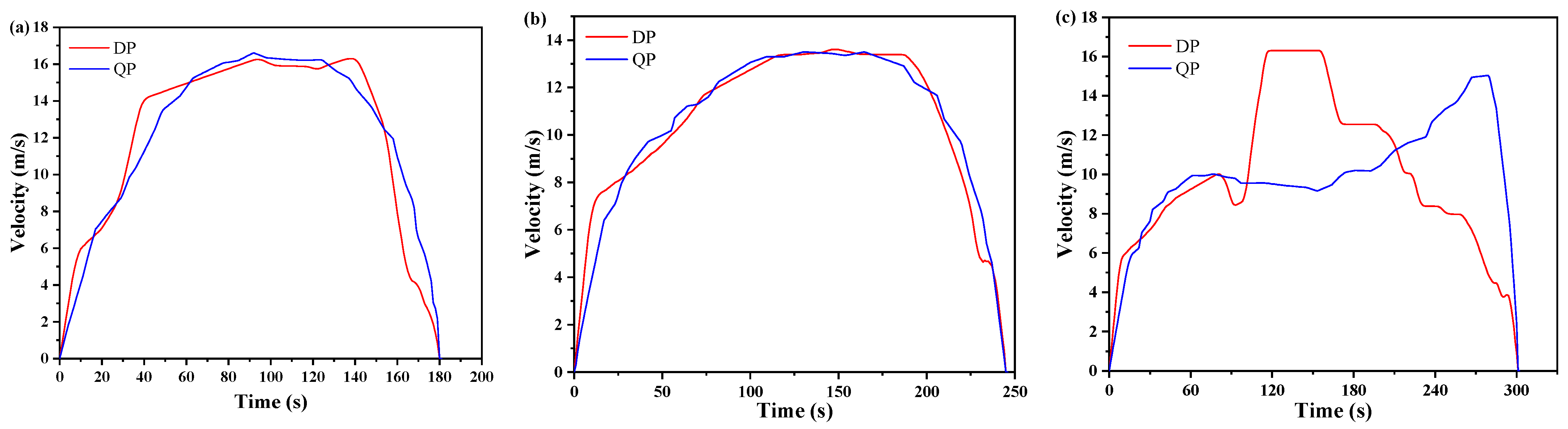
4.2. Analysis of Speed-Planning Results

To validate the performance of the speed-planning method based on the dynamic programming (DP) algorithm, this study selected three different scenarios on a specific road segment in Liuzhou City for testing. The fundamental parameters of each scenario are delineated in

Table 3. Basic parameters for different traffic scenarios.

Traffic Scenario	Scenario 1	Scenario 2	Scenario 2
Number of traffic lights	5	6	7
Distance (m)	2200	2600	3000
Location of traffic lights (m)	250, 900, 1300, 1650, 2200	300, 600, 1000, 1300, 2300, 2600	300, 700, 1000, 1700, 2100, 2500, 3000
Duration of red light (s)	15, 20, 30, 25, 35	25, 30, 25, 30, 20, 30	25, 30, 25, 30, 20, 30, 40
Duration of green light (s)	25, 40, 20, 30, 30	35, 20, 30, 40, 25, 30	35, 20, 30, 40, 25, 30, 20
Duration of traffic signals (s)	40, 60, 50, 55, 65	60, 50, 55, 70, 45, 60	60, 50, 55, 70, 45, 60, 60
Initial times of traffic signals (s)	5, 10, 10, 40, 30	25, 30, 25, 50, 0, 10	15, 30, 50, 20, 5, 45, 10

. Scenario 1: The road spans 2200 m with 5 traffic signals. Scenario 2: The road spans 2600 m with 6 traffic signals. Scenario 3: The road spans 3000 m with 7 traffic signals.

In this paper, dynamic programming (DP) and quadratic programming (QP) are used to optimize the speed of vehicles through traffic signals. Figure 8 illustrates the driving trajectories under different traffic scenarios. The red segments indicate the positions of red traffic lights. Figure 8a shows the driving trajectory for traffic scenario 1, Figure 8b for traffic scenario 2, and Figure 8c for traffic scenario 3. From the figures, it can be observed that both dynamic programming (DP) and quadratic programming (QP) methods enable the vehicle to pass through multiple traffic-signalized intersections without stopping. In the middle section of the trajectory, the trajectory generated by the DP-based method is located above that of the quadratic programming method. However, both methods eventually reach the endpoint simultaneously. This indicates that the DP-based vehicle decelerates more gradually during the approach to the endpoint, allowing the quadratic programming-based vehicle to catch up. Therefore, the DP-based method demonstrates better driving comfort compared to the quadratic programming method. In traffic scenarios 1 and 2, the differences in driving trajectories are relatively small. This is because the number of traffic signals in scenarios 1 and 2 is fewer than that in scenario 3, resulting in less variation in the optimal planning schemes. In traffic scenario 3, when the vehicle passes through the fourth traffic signal, the dynamic programming (DP) method is faster by one red light duration compared to the quadratic programming (QP) method. This is because, when the vehicle passes through the third traffic signal, the DP method achieves a higher speed than the QP method, leading the vehicle to arrive at the fourth traffic signal just before the red light turns on. Consequently, at the fourth traffic signal, the DP method allows the vehicle to pass through one red light duration earlier than the QP method.

Figure 9 illustrates the speed-planning curves for different traffic scenarios: Figure 9a shows the speed-planning curve for traffic scenario 1, Figure 9b shows the speed-planning curve for traffic scenario 2, and Figure 9c shows the speed-planning curve for traffic scenario 3. It can be seen from the figure that in traffic scenes 1 and 2, the speed-planning curves of the two methods are similar, but the speed-planning curve based on dynamic planning is smoother. In traffic scenario 3, the difference between the two speed-planning methods is large. The method based on dynamic planning has a higher speed, which is between 117 s and 155 s, thus enabling the vehicle to quickly pass the fourth traffic light and reach the destination faster.

Table 4. Computational time for speed planning with different algorithms.

Traffic Scenario	Scenario 1	Scenario 2	Scenario 3	Average
DP computational time (s)	17.83	18.67	19.51	18.67
QP computational time (s)	19.01	20.85	22.79	20.88

shows the calculation time of speed planning of different algorithms. It can be seen from the table that the average calculation time based on the dynamic programming algorithm is 18.67 s, which is less than 20.88 s based on the quadratic programming. Among them, the calculation time used by traffic scenario 1 is the smallest, which is 17.83 s, and the calculation time used by traffic scenario 3 is the largest, which is 19.51 s. This is because the trajectory calculated by traffic scenario 3 is 800 m longer than that of scenario 1, and the number of traffic lights is also 2 more than that of scenario 1. Therefore, the speed-planning method based on dynamic planning constructed in this paper performs better when dealing with complex traffic scenarios, can well balance the computational efficiency and the complexity of the model, and can achieve more efficient speed planning.

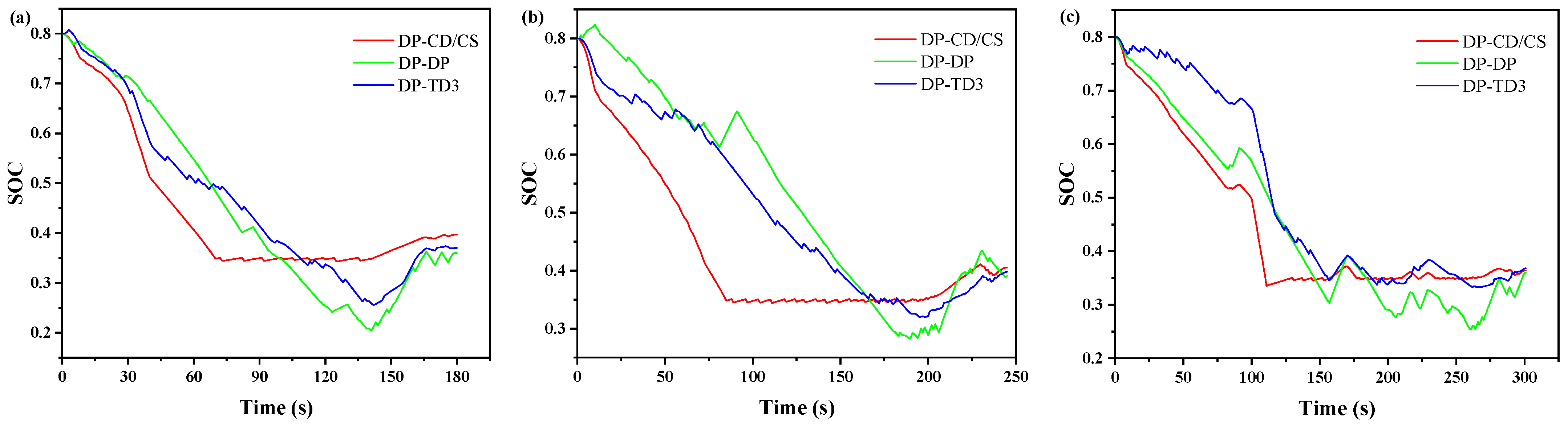
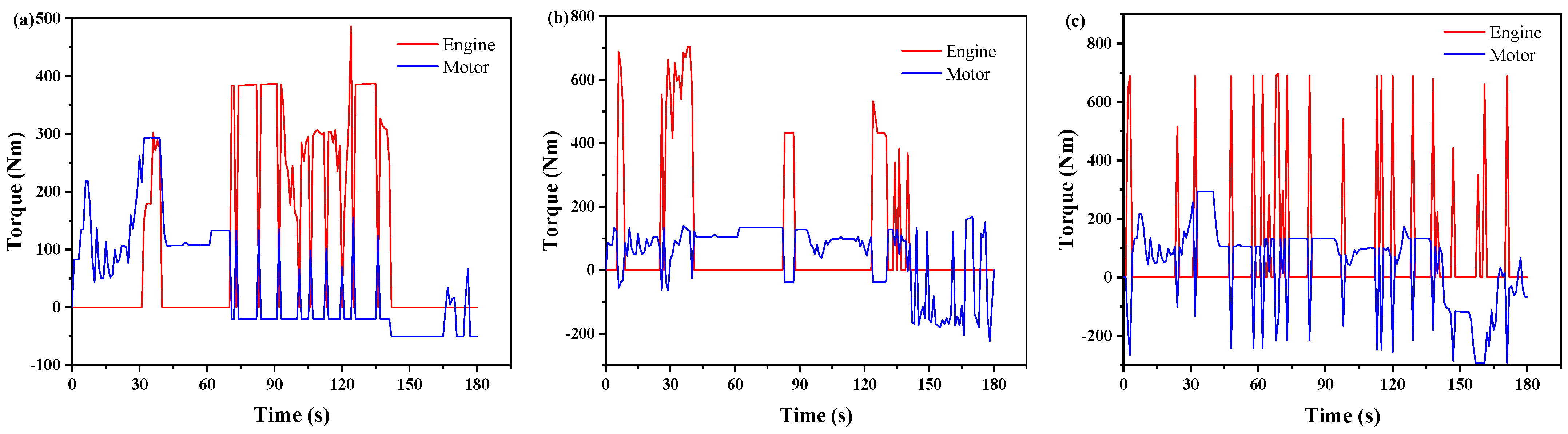
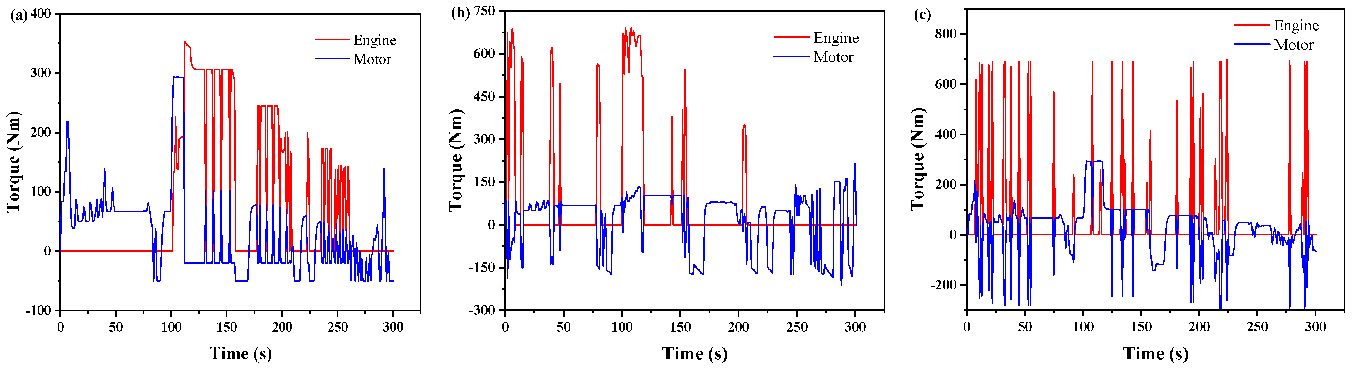
4.3. Analysis of Fuel Economy

Based on the analysis of the speed-planning models presented above, it is verified that the performance of the speed-planning model based on dynamic programming outperforms that of the quadratic programming method. This section analyzes fuel economy using the dynamic programming-based speed-planning model as the foundation. To validate the efficacy of the hierarchical energy management strategy employing the DP-TD3 algorithm, this paper simultaneously develops both the DP-CD/CS model and the DP-DP model. To accurately describe the fuel economy of vehicles, this paper defines the fuel-saving rate, $\mu ={\displaystyle \frac{|A-B|}{A}}\times 100\%$, where A represents the fuel consumption value based on the DP-CD/CS method, and B represents the fuel consumption value of the optimized method.

Table 5. Fuel consumption for traffic scenarios 1, 2, and 3.

Traffic Scenario	Method	Final Value of SOC	Fuel Consumption Value (L/100 km)	Fuel Saving-Rate Value (%)
Traffic scenario 1	DP-CD/CS	0.39	11.85	0
	DP-DP	0.36	9.08	23.38
	DP-TD3	0.37	9.83	17.05
Traffic scenario 2	DP-CD/CS	0.40	11.17	0
	DP-DP	0.39	9.13	18.26
	DP-TD3	0.40	9.79	12.35
Traffic scenario 3	DP-CD/CS	0.36	11.37	0
	DP-DP	0.36	9.04	20.49
	DP-TD3	0.37	9.73	14.42

presents the fuel consumption for different traffic scenarios. In traffic scenario 1, the DP-CD/CS model exhibits the highest fuel consumption at 11.85 L/100 km, while the DP-DP model achieves the lowest fuel consumption at 9.08 L/100 km, with a fuel-saving rate of 23.38%. The DP-TD3 model’s fuel consumption falls in between, at 9.83 L/100 km, with a fuel-saving rate of 17.05%. In traffic scenario 2, the fuel consumption of the DP-TD3 model is 9.79 L/100 km, corresponding to a fuel-saving rate of 12.35%. In traffic scenario 3, the DP-TD3 model’s fuel consumption is 9.73 L/100 km, with a fuel-saving rate of 14.42%. Based on the above data, it can be seen that the average fuel saving of DP-DP model is 20.71% and the average fuel saving of DP-TD3 model is 14.61%. The DP-DP model represents a globally optimal method, with the fuel-saving rate of the DP-TD3 model trailing by merely 6.10% in comparison. Consequently, the hierarchical energy management strategy rooted in the DP-TD3 algorithm demonstrates relative excellence, effectively curtailing vehicle fuel consumption and thereby enhancing fuel economy.

Figure 10 shows the SOC change curves under different traffic scenarios. Figure 10a shows the SOC variation curve for traffic scenario 1. The SOC of the DP-CD/CS model decreases rapidly from 0.8 at the beginning and finally stays near 0.35. This is due to the fact that the SOC is dominated by the motor drive between 0.8 and 0.35, which has been consuming electrical energy. When the SOC is below 0.35, the engine starts to work and drives the vehicle together with the electric motor. And the SOC has a slow rebound after 135 s, which is due to the slow deceleration braking of the truck and partial energy recovery by the motor. The SOC of the DP-DP model is slowly decreasing between 0 s and 140 s, and then slowly increasing between 140 s and 180 s. This is due to the acceleration of the truck before 140 s and the deceleration of the truck after 140 s. During the deceleration phase, the motor performs energy recovery. The SOC trends of the DP-TD3 model are basically the same as those of the DP-DP model. The fuel consumption of the DP-TD3 model is marginally lower than that of the DP-DP model. Figure 10b shows the SOC change curve of traffic scenario 2. The SOC value of the DP-TD3 model dropped from the initial value of 0.8 to 0.40, reaching the lowest point of 0.32 at 200 s, and then slowly increased through energy recovery. Figure 10c shows the SOC change curve for traffic scenario 3. The SOC value of the DP-TD3 model decreased from the initial value of 0.8 to 0.37, and it fluctuated at 170 s and 230 s due to the large change in the vehicle’s speed at these two places. The validation of the three traffic scenarios shows that the DP-TD3 model can adapt to different working conditions with high stability. Figure 11 displays the convergence curves of the TD3 algorithm training. Specifically, Figure 11a illustrates the convergence curve for traffic scenario 1, Figure 11b for traffic scenario 2, and Figure 11c for traffic scenario 3. It is evident from the figures that the energy management model, employing the TD3 algorithm, reaches convergence after approximately 50 training iterations. Moreover, the post-convergence fluctuation is minimal, indicating the attainment of an optimal solution. Therefore, the power allocation model of the TD3 algorithm constructed in this article can adapt to the calculation of different working conditions and has strong adaptability.

Figure 12 illustrates the torque distribution of the engine and motor for traffic scenario 1. Specifically, Figure 12a presents the torque distribution for the DP-CD/CS model. It is apparent from the figure that the model predominantly utilizes the motor to propel the vehicle, while the engine is engaged solely to supply energy when power consumption reaches a predetermined threshold. Figure 12b presents the torque distribution of the engine and motor for the DP-DP model. The figure vividly demonstrates the collaborative effort between the motor and engine to propel the vehicle, with a noticeable reduction in engine usage. Consequently, the fuel consumption of this model is minimal. In contrast, Figure 12c displays the torque distribution of the engine and motor for the DP-TD3 model. It is evident from the figure that this model exhibits a higher reliance on the engine, resulting in slightly elevated fuel consumption compared to the DP-DP model. Figure 13a illustrates the engine operating points map for traffic scenario 1. Notably, the DP-CD/CS model consistently exhibits engine operating points within the high fuel consumption rate region, while the DP-DP model exclusively resides in the low fuel consumption rate region. In contrast, the engine operating points of the DP-TD3 model span both low and high fuel consumption rate regions. Consequently, the fuel consumption of the DP-TD3 model exceeds that of the DP-DP model, measuring at 9.83 L/100 km. Nevertheless, it closely approximates the fuel consumption of the globally optimal DP-DP model, which stands at 9.08 L/100 km. Figure 14 illustrates the torque distribution of the engine and motor for traffic scenario 2. Figure 13b displays the engine operating point map for traffic scenario 2. Figure 15 presents the torque distribution of the engine and motor for traffic scenario 3. Figure 13c illustrates the engine operating point map for traffic scenario 3. Our analysis of the engine operating points from traffic scenarios 2 and 3 reveals that the engine predominantly operates within the high-efficiency interval, characterized by low fuel consumption rates. Hence, the DP-TD3 control strategy developed in this study effectively enhances the fuel economy of the hybrid electric truck.

4.4. Hardware-in-the-Loop Experimental Verification

In this paper, experimental validation is conducted utilizing the chassis power domain hardware-in-the-loop (HIL) test machine, as depicted in Figure 16. The hardware components of the hardware-in-the-loop testing system for the chassis power domain primarily include the chassis test rig, control cabinet, monitor, and computer. The software components mainly consist of ConfigurationDesk (6.5) and ControlDesk (7.2). ConfigurationDesk is used for system configuration and code generation, while ControlDesk is responsible for connecting with the target hardware, real-time monitoring, and recording various operating states of the vehicle. The chassis power domain hardware-in-the-loop tester is designed to control the engine, motor, transmission, and vehicle models by inputting loads, control signals, and bus interaction information, so as to realize the verification of control algorithms for the engine controller, motor controller, transmission controller, and electronic braking system controller. The basic parameters of the chassis power domain hardware-in-the-loop tester are shown in

Table 6. Basic parameters of the chassis power domain hardware-in-the-loop tester.

Hardware	Parameter
Processor	3.8 GHz frequency, 16 GB RAM memory.
DS2680 board	44-channel AI, 64-channel AO, 60-channel DI, 56-channel DO, 32-channel FI, 24-channel RO.
DS2690 board	20-channel DI, 20-channel DO, 20-channel DI/DO.
DS2671 board	4 CAN bus emulation channels.
Programmable power supply	Power, 1.5 KW; voltage, 0 V-52 V; current, 0 A-60 A.

.

In this paper, hardware-in-the-loop testing is performed for traffic scenario 1. Figure 17 displays the test results. It is apparent from the figure that the truck’s speed curve, SOC curve, and engine operating point align closely with the simulation results, albeit with some local deviations. The root-mean-square error of the speed curve is 0.0846 m/s, and the root-mean-square error of the SOC curve is 0.0022. The fuel consumption of the hardware-in-the-loop test is 9.97 L/100 km, which is 0.14 L/100 km more than that of the simulation result. This small deviation between test and simulation results is due to the fact that the simulation model is a partially simplified vehicle model. The simplified truck model does not exactly match the actual vehicle, and the driver’s tracking speed is partially biased. Hence, the hardware-in-the-loop test results serve to validate that the hierarchical energy management strategy proposed in this paper is effective in enhancing the fuel economy of plug-in hybrid electric trucks.

5. Conclusions

In this paper, a hierarchical energy management strategy based on the DP-TD3 algorithm is devised. The integration of speed planning and energy management issues into a co-optimization approach aims to enhance the passability and fuel economy of plug-in hybrid electric trucks across multiple successive traffic light intersections.

(1)

In the upper layer, a speed-planning model for the DP algorithm is constructed to plan the vehicle trajectory according to the position, phase, and timing of traffic signals in order to avoid stopping the vehicle due to red lights. The speed-planning model adeptly converts the nonlinear constraints associated with traffic signals into time-varying constraints. This strategic transformation effectively diminishes the model’s complexity while significantly enhancing computational efficiency.

(2)

In the lower layer, an energy management strategy is devised using the TD3 algorithm to efficiently allocate power for the plug-in hybrid electric truck. This strategy operates through the interaction between the TD3 agent and the environment.

(3)

The simulation results demonstrate that the DP-TD3 method significantly decreases the fuel consumption of plug-in hybrid electric trucks. In comparison to the DP-CD/CS method, there is a fuel saving of 17.05% in traffic scenario 1 and 12.35% in traffic scenario 2. The fuel saving in traffic scenario 3 is 14.42%, with an average of 14.61%.

(4)

The hardware-in-the-loop test results reveal that the fuel consumption of the DP-TD3 method is 9.97 L/100 km, a finding that aligns closely with the simulation results.

Therefore, the DP-TD3 method developed in this study effectively addresses the issue of parking for plug-in hybrid electric trucks at traffic light intersections, thereby significantly enhancing vehicle fuel economy.

In the future, we can integrate real-time traffic conditions and traffic signal state predictions, leveraging technologies such as V2X for dynamic adjustments to enhance the adaptability of energy management strategies. Additionally, this study only considers the speed-planning problem for a single vehicle. However, in real-world road scenarios, platoon driving is more common. Future research can focus on achieving coordinated control of energy management and speed optimization within vehicle platoons.

References

1. Jia, C.C.; He, H.W.; Zhou, J.M.; Li, J.W.; Wei, Z.B.; Li, K.A. A novel health-aware deep reinforcement learning energy management for fuel cell bus incorporating offline high-quality experience. Energy 2023, 282, 12892. [Google Scholar] [CrossRef]
2. Hu, J.; Shao, Y.L.; Sun, Z.X.; Wang, M.; Bared, J.; Huang, P. Integrated optimal eco-driving on rolling terrain for hybrid electric vehicle with vehicle-infrastructure communication. Transp. Res. Part C Emerg. Technol. 2016, 68, 228–244. [Google Scholar] [CrossRef]
3. Liu, S.C.; Sun, H.W.; Yu, H.T.; Miao, J.; Zheng, C.; Zhang, X.W. A framework for battery temperature estimation based on fractional electro-thermal coupling model. J. Energy Storage 2023, 63, 107042. [Google Scholar] [CrossRef]
4. Li, X.P.; Zhou, J.M.; Guan, W.; Jiang, F.; Xie, G.M.; Wang, C.F.; Zheng, W.G.; Fang, Z.J. Optimization of Brake Feedback Efficiency for Small Pure Electric Vehicles Based on Multiple Constraints. Energies 2023, 16, 6531. [Google Scholar] [CrossRef]
5. Meng, X.Y.; Cassandras, C.G. Eco-Driving of Autonomous Vehicles for Nonstop Crossing of Signalized Intersections. IEEE Trans. Autom. Sci. Eng. 2022, 19, 320–331. [Google Scholar] [CrossRef]
6. Li, J.; Liu, Y.G.; Zhang, Y.J.; Lei, Z.Z.; Chen, Z.; Li, G. Data-driven based eco-driving control for plug-in hybrid electric vehicles. J. Power Sources 2021, 498, 229916. [Google Scholar] [CrossRef]
7. Xu, N.; Li, X.H.; Yue, F.L.; Jia, Y.F.; Liu, Q.; Zhao, D. An Eco-Driving Evaluation Method for Battery Electric Bus Drivers Using Low-Frequency Big Data. IEEE Trans. Intell. Transp. Syst. 2023, 24, 9296–9308. [Google Scholar] [CrossRef]
8. Huang, Y.H.; Ng, E.C.Y.; Zhou, J.L.; Surawski, N.C.; Chan, E.F.C.; Hong, G. Eco-driving technology for sustainable road transport: A review. Renew. Sustain. Energy Rev. 2018, 93, 596–609. [Google Scholar] [CrossRef]
9. Sankar, G.S.; Kim, M.; Han, K. Data-Driven Leading Vehicle Speed Forecast and Its Application to Ecological Predictive Cruise Control. IEEE Trans. Veh. Technol. 2022, 71, 11504–11514. [Google Scholar] [CrossRef]
10. Huang, K.; Yang, X.F.; Lu, Y.; Mi, C.C.; Kondlapudi, P. Ecological Driving System for Connected/Automated Vehicles Using a Two-Stage Control Hierarchy. IEEE Trans. Intell. Transp. Syst. 2018, 19, 2373–2384. [Google Scholar] [CrossRef]
11. Pan, C.; Li, Y.; Huang, A.; Wang, J.; Liang, J. Energy-optimized adaptive cruise control strategy design at intersection for electric vehicles based on speed planning. Sci. China-Technol. Sci. 2023, 66, 3504–3521. [Google Scholar] [CrossRef]
12. Li, J.; Fotouhi, A.; Pan, W.J.; Liu, Y.G.; Zhang, Y.J.; Chen, Z. Deep reinforcement learning-based eco-driving control for connected electric vehicles at signalized intersections considering traffic uncertainties. Energy 2023, 279, 128139. [Google Scholar] [CrossRef]
13. Sun, C.; Guanetti, J.; Borrelli, F.; Moura, S.J. Optimal Eco-Driving Control of Connected and Autonomous Vehicles Through Signalized Intersections. IEEE Internet Things J. 2020, 7, 3759–3773. [Google Scholar] [CrossRef]
14. Guo, J.Q.; He, H.W.; Li, J.W.; Liu, Q.W. Real-time energy management of fuel cell hybrid electric buses: Fuel cell engines friendly intersection speed planning. Energy 2021, 226, 120440. [Google Scholar] [CrossRef]
15. Wei, X.D.; Leng, J.H.; Sun, C.; Huo, W.W.; Ren, Q.; Sun, F.C. Co-optimization method of speed planning and energy management for fuel cell vehicles through signalized intersections. J. Power Sources 2022, 518, 230598. [Google Scholar] [CrossRef]
16. Liu, X.; Yang, C.B.; Meng, Y.M.; Zhu, J.H.; Duan, Y.J.; Chen, Y.J. Hierarchical energy management of plug-in hybrid electric trucks based on state-of-charge optimization. J. Energy Storage 2023, 72, 107999. [Google Scholar] [CrossRef]
17. Ibrahim, O.; Bakare, M.S.; Amosa, T.I.; Otuoze, A.O.; Owonikoko, W.O.; Ali, E.M.; Adesina, L.M.; Ogunbiyi, O. Development of fuzzy logic-based demand-side energy management system for hybrid energy sources. Energy Convers. Manag. X 2023, 18, 100354. [Google Scholar] [CrossRef]
18. Fernandez, A.M.; Kandidayeni, M.; Boulon, L.; Chaoui, H. An Adaptive State Machine Based Energy Management Strategy for a Multi-Stack Fuel Cell Hybrid Electric Vehicle. IEEE Trans. Veh. Technol. 2020, 69, 220–234. [Google Scholar] [CrossRef]
19. Qi, C.Y.; Song, C.X.; Xiao, F.; Song, S.X. Generalization ability of hybrid electric vehicle energy management strategy based on reinforcement learning method. Energy 2022, 250, 123826. [Google Scholar] [CrossRef]
20. Wang, W.D.; Guo, X.H.; Yang, C.; Zhang, Y.B.; Zhao, Y.L.; Huang, D.G.; Xiang, C.L. A multi-objective optimization energy management strategy for power split HEV based on velocity prediction. Energy 2022, 238, 121714. [Google Scholar] [CrossRef]
21. Pan, W.J.; Wu, Y.T.; Tong, Y.; Li, J.; Liu, Y.G. Optimal rule extraction-based real-time energy management strategy for series-parallel hybrid electric vehicles. Energy Convers. Manag. 2023, 293, 117474. [Google Scholar] [CrossRef]
22. Chen, H.; Guo, G.; Tang, B.B.; Hu, G.; Tang, X.L.; Liu, T. Data-driven transferred energy management strategy for hybrid electric vehicles via deep reinforcement learning. Energy Rep. 2023, 10, 2680–2692. [Google Scholar] [CrossRef]
23. Deng, K.; Liu, Y.X.; Hai, D.; Peng, H.J.; Löwenstein, L.; Pischinger, S.; Hameyer, K. Deep reinforcement learning based energy management strategy of fuel cell hybrid railway vehicles considering fuel cell aging. Energy Convers. Manag. 2022, 251, 115030. [Google Scholar] [CrossRef]
24. Gissing, J.; Themann, P.; Baltzer, S.; Lichius, T.; Eckstein, L. Optimal Control of Series Plug-In Hybrid Electric Vehicles Considering the Cabin Heat Demand. IEEE Trans. Control Syst. Technol. 2016, 24, 1126–1133. [Google Scholar] [CrossRef]
25. Peng, H.J.; Chen, Z.; Li, J.X.; Deng, K.; Dirkes, S.; Gottschalk, J.; Ünlübayir, C.; Thul, A.; Löwenstein, L.; Pischinger, S.; et al. Offline optimal energy management strategies considering high dynamics in batteries and constraints on fuel cell system power rate: From analytical derivation to validation on test bench. Appl. Energy 2021, 282, 116152. [Google Scholar] [CrossRef]
26. Xiang, C.L.; Ding, F.; Wang, W.D.; He, W.; Qi, Y.L. MPC-based energy management with adaptive Markov-chain prediction for a dual-mode hybrid electric vehicle. Sci. China Technol. Sci. 2017, 60, 737–748. [Google Scholar] [CrossRef]
27. Xu, F.G.; Shen, T.L. Look-Ahead Prediction-Based Real-Time Optimal Energy Management for Connected HEVs. IEEE Trans. Veh. Technol. 2020, 69, 2537–2551. [Google Scholar] [CrossRef]
28. Deng, L.; Li, S.; Tang, X.L.; Yang, K.; Lin, X.K. Battery thermal- and cabin comfort-aware collaborative energy management for plug-in fuel cell electric vehicles based on the soft actor-critic algorithm. Energy Convers. Manag. 2023, 283, 116889. [Google Scholar] [CrossRef]
29. Tang, X.L.; Zhou, H.T.; Wang, F.; Wang, W.D.; Lin, X.K. Longevity-conscious energy management strategy of fuel cell hybrid electric Vehicle Based on deep reinforcement learning. Energy 2022, 238, 121593. [Google Scholar] [CrossRef]
30. Qi, C.Y.; Zhu, Y.W.; Song, C.A.X.; Yan, G.F.; Wang, D.; Xiao, F.; Zhang, X.; Cao, J.W.; Song, S.X. Hierarchical reinforcement learning based energy management strategy for hybrid electric vehicle. Energy 2022, 238, 121703. [Google Scholar] [CrossRef]
31. Xiong, R.; Cao, J.Y.; Yu, Q.Q. Reinforcement learning-based real-time power management for hybrid energy storage system in the plug-in hybrid electric vehicle. Appl. Energy 2018, 211, 538–548. [Google Scholar] [CrossRef]
32. Chang, C.C.; Zhao, W.Z.; Wang, C.Y.; Song, Y.D. A Novel Energy Management Strategy Integrating Deep Reinforcement Learning and Rule Based on Condition Identification. IEEE Trans. Veh. Technol. 2023, 72, 1674–1688. [Google Scholar] [CrossRef]
33. Qi, X.W.; Luo, Y.D.; Wu, G.Y.; Boriboonsomsin, K.; Barth, M. Deep reinforcement learning enabled self-learning control for energy efficient driving. Transp. Res. Part C Emerg. Technol. 2019, 99, 67–81. [Google Scholar] [CrossRef]
34. Huang, R.C.; He, H.W.; Zhao, X.Y.; Wang, Y.L.; Li, M.L. Battery health-aware and naturalistic data-driven energy management for hybrid electric bus based on TD3 deep reinforcement learning algorithm. Appl. Energy 2022, 321, 119353. [Google Scholar] [CrossRef]
35. Zhang, Y.J.; Huang, Y.J.; Chen, Z.; Li, G.; Liu, Y.G. A Novel Learning-Based Model Predictive Control Strategy for Plug-In Hybrid Electric Vehicle. IEEE Trans. Transp. Electrif. 2022, 8, 23–35. [Google Scholar] [CrossRef]
36. Fujimoto, S.; van Hoof, H.; Meger, D. Addressing Function Approximation Error in Actor-Critic Methods. In Proceedings of the 35th International Conference on Machine Learning (ICML), Stockholm, Sweden, 10–15 July 2018. [Google Scholar] [CrossRef]
37. Zhou, L.Q.; Yang, D.P.; Zeng, X.H.; Zhang, X.M.; Song, D.F. Multi-objective real-time energy management for series-parallel hybrid electric vehicles considering battery life. Energy Convers. Manag. 2023, 290, 117234. [Google Scholar] [CrossRef]
38. Xie, S.B.; Hu, X.S.; Qi, S.W.; Tang, X.L.; Lang, K.; Xin, Z.K.; Brighton, J. Model predictive energy management for plug-in hybrid electric vehicles considering optimal battery depth of discharge. Energy 2019, 173, 667–678. [Google Scholar] [CrossRef]
Figure 1. Structure of the plug-in hybrid electric truck.
Energies 17 06022 g001
Figure 2. Engine fuel consumption rate map.
Energies 17 06022 g002
Figure 3. Motor efficiency map.
Energies 17 06022 g003
Figure 4. Schematic diagram of vehicles passing through traffic lights.
Energies 17 06022 g004
Figure 5. Control strategy framework.
Energies 17 06022 g005
Figure 6. Upper and lower reference trajectories of the vehicle.
Energies 17 06022 g006
Figure 7. Network structure of TD3 algorithm.
Energies 17 06022 g007
Figure 8. Driving trajectory curves for different traffic scenarios: (a) scenario 1, (b) scenario 2, and (c) scenario 3.
Energies 17 06022 g008
Figure 9. Speed-planning curves for different traffic scenarios: (a) scenario 1, (b) scenario 2, and (c) scenario 3.
Energies 17 06022 g009
Figure 10. Variation curve of SOC for (a) scenario 1, (b) scenario 2, and (c) scenario 3.
Energies 17 06022 g010
Figure 11. Convergence curve for (a) scenario 1, (b) scenario 2, and (c) scenario 3.
Energies 17 06022 g011
Figure 12. Torque distribution of engine and motor for traffic scenario 1: (a) DP-CD/CS, (b) DP-DP, and (c) DP-TD3.
Energies 17 06022 g012
Figure 13. Engine operating point map for (a) scenario 1, (b) scenario 2, and (c) scenario 3.
Energies 17 06022 g013
Figure 14. Torque distribution of engine and motor for traffic scenario 2: (a) DP-CD/CS, (b) DP-DP, and (c) DP-TD3.
Energies 17 06022 g014
Figure 15. Torque distribution of engine and motor for traffic scenario 3: (a) DP-CD/CS, (b) DP-DP, and (c) DP-TD3.
Energies 17 06022 g015
Figure 16. Chassis power domain hardware-in-the-loop test system.
Energies 17 06022 g016
Figure 17. Comparison of simulation and test results: (a) speed curve, (b) SOC curve, and (c) engine operating point map.
Energies 17 06022 g017