A Rotating Tidal Current Controller and Energy Router Siting and Capacitation Method Considering Spatio-Temporal Distribution

Abstract

As the proportion of new energy access increases year by year, the resulting energy imbalance and voltage/trend distribution complexity of the distribution network system in the spatio-temporal dimension become more and more prominent. The joint introduction of electromagnetic rotary power flow controller (RPFC) and energy router (ER) can improve the high proportion of new active distribution network (ADN) consumption and power supply reliability from both spatial and temporal dimensions. To this end, the paper proposes an ADN expansion planning method considering RPFC and ER access. A two-layer planning model for RPFC and ER based on spatio-temporal characteristics is established, with the upper model being the siting and capacity-setting layer, which takes the investment and construction cost of RPFC and ER as the optimization objective, and the lower model being the optimal operation layer, which takes the lowest operating cost of the distribution network as the objective. The planning model is solved by a hybrid optimization algorithm with improved particle swarm and second-order cone planning. The proposed planning model and solving algorithm are validated with the IEEE33 node example, and the results show that the joint access of RPFC and ER can effectively improve the spatial-temporal distribution of voltage in the distribution network and has the lowest equivalent annual value investment and operation cost.

1. Introduction

With the urgent need to accommodate a high proportion of distributed renewable energy integration, it is essential to enhance the capacity and reliability of active distribution networks (ADN) from both spatial and temporal dimensions [1]. Current distribution systems face challenges such as weak grid structures, uneven local load distribution, and inadequate power supply capabilities. As the share of renewable energy increases each year, issues of energy imbalance, complex voltage and power flow distribution across spatial and temporal dimensions within the distribution network become increasingly prominent [2]. Flexible Interconnection Devices (FID) based on power electronics can enable flexible interconnections in medium- and low-voltage distribution networks, such as through smart soft switches (SOP), electromagnetic rotary power flow controller (RPFC), and energy routers (ER). These devices facilitate loop operations between AC and DC distribution feeders, enabling functions such as power transfer, load balancing, loss reduction, fault isolation, and power restoration. However, power-electronic-based FIDs also have drawbacks, including limited shock tolerance, challenging maintenance, and high costs, which significantly restrict their wider application in medium- and low-voltage distribution networks. The electromagnetic rotary power flow controller (RPFC) [3], using a wound motor structure, offers advantages of high shock resistance and reliability, providing the same functions as power-electronic-based FIDs within distribution networks. It also has distinct benefits: a response time on the order of seconds, simple control, strong continuity, no harmonic output, and lower costs. Therefore, establishing a flexible AC/DC active distribution network (ADN) using RPFC and ER [4] presents clear advantages over ADN solutions based solely on power-electronic devices [5]. To fully leverage the benefits that widespread integration of RPFC and ER can bring to ADNs, it is crucial to study and develop expansion planning models that consider RPFC and ER integration [6].

The RPFC is typically installed between two looped lines in a distribution system, enabling adjustable power transfer of any magnitude and direction between these looped lines to optimize the operation of the distribution network [7]. In terms of flexible interconnections within the distribution network, research on the siting and sizing of RPFC remains limited. Existing planning and configuration schemes based on soft open points (SOP) in interconnected distribution networks provide a useful reference. Reference [8] proposes an optimized configuration method for SOPs in active distribution networks, utilizing an improved sensitivity analysis approach. This method employs a second-order cone programming algorithm to solve the siting and sizing optimization model for SOPs under enhanced sensitivity calculations. The case study results demonstrate that optimized SOP configuration effectively reduces the annual operational costs of the distribution network and improves system voltage stability. Building on this, Reference [9] considers the loss characteristics of transformers and SOPs within a two-layer model to determine SOP locations. The upper layer minimizes annual total costs, while the lower layer minimizes system losses. This approach was validated on interconnected systems with IEEE 22-bus and IEEE 15-bus nodes, showing that the proposed control strategy significantly reduces system losses while maintaining minimal annual investment costs, thereby enhancing both economic efficiency and reliability. Reference [10] further develops an expansion planning study for ADNs that incorporates SOP access. This research addresses the coordinated siting and sizing of new or expanded substations, new lines, SOPs, distributed generation (DG), energy storage systems (ESS), and reactive power compensation devices.

The above literature indicates that reasonable planning for the location and capacity of the RPFC is crucial for improving ADN operational efficiency and promoting flexible development in distribution networks. However, the RPFC can only optimize voltage and power flow distribution across the active distribution network spatially [11]. The ER, on the other hand, provides flexibility support to external systems on a node basis. By enabling optimized scheduling of flexible resources at its ports, the ER addresses energy imbalances in the time dimension, power quality issues, and the reliability of power supply for critical loads. Coordinated operation of RPFC and ER enhances the ADN’s ability to accommodate high proportions of renewable energy and ensures reliable power supply from both spatial and temporal dimensions [12,13]. References propose an optimal planning method for ER clusters in distribution networks, which includes the unified planning of ER groups and other distributed resources within the network [14,15]. Simulation validations confirm the method’s effectiveness, providing a planning reference for distribution networks integrating various new types of generation and load.

Currently, extensive research has been conducted on the siting and planning of flexible interconnection devices and ERs [16,17]. However, in terms of coordinated spatiotemporal planning, Reference [18] proposes an ESS-SOP network collaborative planning method that considers the integration of flexible loads. This approach takes into account the temporal characteristics of distributed generation and flexible loads, constructing a collaborative planning model for ESS-SOP and network architecture, which was validated on an IEEE 33-bus system. Reference [19] further integrates the operational characteristics of ESS and SOP, introducing a three-layer model for ESS and SOP. The upper and middle layers aim to minimize the combined investment and operational costs for siting and capacity planning, while the lower layer targets daily average flexibility in optimizing operational scheduling. A hybrid optimization algorithm was employed to solve this model, with case studies validating the model’s rationality and effectiveness for SOP and ESS coordinated planning. To date, however, no research team has extended the collaborative function of RPFC and ER into ADN planning scheme design.

Based on existing research, this paper proposes an ADN expansion planning method that considers the spatiotemporal regulation characteristics of RPFC and ER. First, an ADN two-stage expansion planning model is developed with the objective function of minimizing the annualized comprehensive cost, taking into account the integration of RPFC and ER. Given that the proposed model represents a nonlinear programming problem, a hybrid algorithm combining improved particle swarm optimization (IPSO) and second-order cone programming (SOCP) is introduced to solve it. The feasibility and effectiveness of the proposed planning model and solution algorithm are then analyzed and validated through a case study on a 33-bus ADN system.

The main innovations of this paper are as follows:

(1)

Model Construction: This work presents the first construction of a grid planning model that includes the RPFC output model and associated constraints, providing a reference framework for subsequent RPFC planning methodologies.

(2)

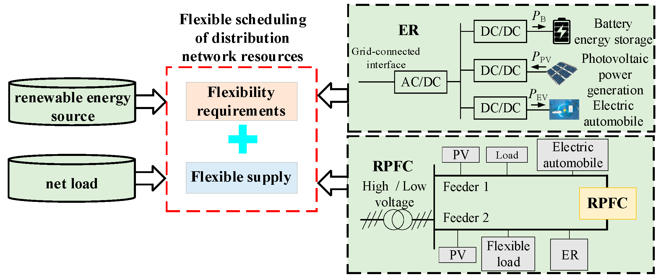
Application Scenario Innovation: The paper introduces a novel siting and planning model that incorporates the hybrid integration of RPFC and ER into distribution networks, offering a new reference for specific distribution network planning approaches.

(3)

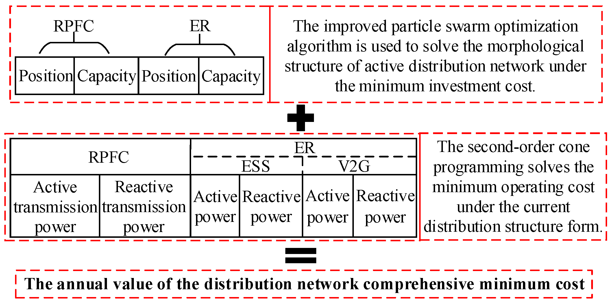
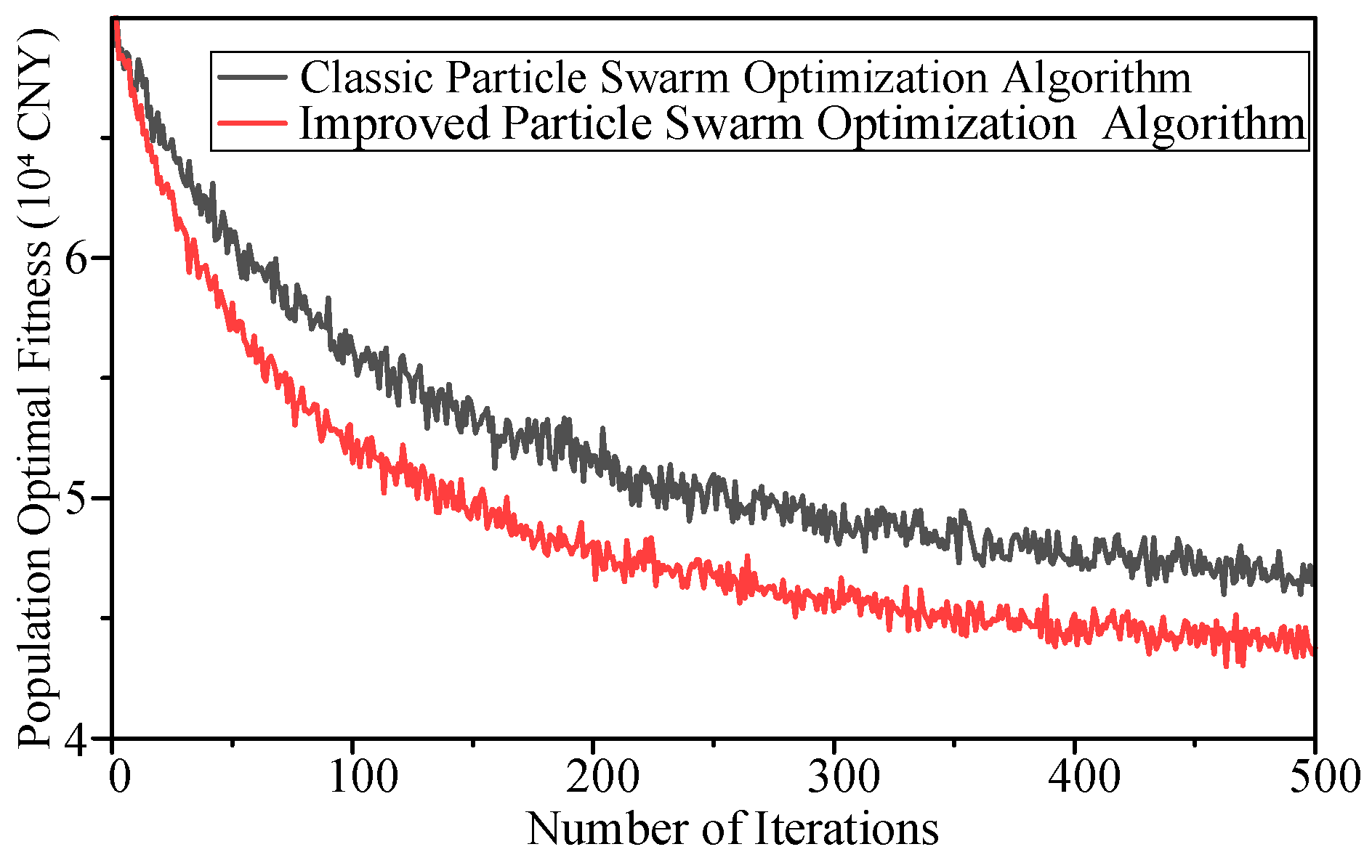
Solution Design for the Dual-Layer Model: A hybrid method combining improved particle swarm optimization (IPSO) and second-order cone programming (SOCP) is applied to solve the RPFC and ER dual-layer model. This approach is validated through simulation on an IEEE 33-bus system, demonstrating the effectiveness of the proposed solution.

2. Two-Layer Planning Modeling of RPFC and ER Based on Spatio-Temporal Properties

The ADN expansion planning scheme with RPFC and ER integration is shown in Figure 1. During the planning process, branch flexibility primarily considers the optimal location and capacity of the RPFC, while node flexibility focuses on the optimal location and capacity of the ER (with a four-port ER being the primary focus of this analysis). This approach aims to maximize the system’s flexibility demand and flexibility supply functions.

Based on the access requirements shown in Figure 1, a dual-layer planning scheme is designed in Figure 2. First, the siting and sizing of the RPFC and ER are treated as the upper-layer model, which optimizes the equivalent annual investment cost for various capacities and locations. When device capacity is low, it does not sufficiently enhance system flexibility; however, larger capacities significantly improve operational flexibility but result in higher costs. Therefore, the upper-layer model aims to minimize the combined investment cost for both RPFC and ER, providing initial siting and sizing results to the lower layer.

The lower-layer model focuses on optimizing operational flexibility in the distribution network. Based on the RPFC and ER configuration plan from the upper layer, it minimizes operational costs across multiple typical daily scenarios by solving for the transmission power in RPFC-connected lines and the charge/discharge power at ER-connected nodes within the interconnected distribution network. These operational costs are then communicated back to the upper layer. This iterative process between the two layers ultimately yields an optimal solution that satisfies both operational and configuration requirements.

2.1. Upper Layer Model

2.1.1. Upper Model Objective Function

The objective function of the upper-layer model is to minimize the annualized investment costs over the planning period for the Active Distribution Network (ADN). This includes the investment cost for the RPFC F_RPFC, the investment cost of ER F_ER(including the construction cost of the ER F_ERD and the supporting DG construction cost F_DG, ES construction cost F_ES, V2G construction cost F_V2G), as well as the civil engineering cost, F_CE. The expression is as follows:

$$\min F_1={\theta }^{\mathrm{RPFC}}{F}_{\mathrm{RPFC}}+{\theta }^{\mathrm{ER}}{F}_{\mathrm{ER}}+{\theta }^{\mathrm{CE}}{F}_{\mathrm{CE}}$$

(1)

$$F_{\mathrm{ER}}=F_{\mathrm{ERD}}+F_{\mathrm{DG}}+F_{\mathrm{ESS}}+F_{\mathrm{V}2\mathrm{G}}$$

(2)

$$\theta ={\displaystyle \frac{d(1+d{)}^{L_{\mathrm{T}}x}}{(1+d{)}^{L_{\mathrm{T}}x}-1}},x\in \left\{\mathrm{RPFC},\mathrm{ER},\mathrm{CE}\right\}$$

(3)

where: θ is the equal-year-value operator, which is used to convert total costs to equal-year-value costs; where d and L_T are the discount rate and the life cycle of the asset, respectively.

2.1.2. Upper Model Constraints

(1)

RPFC installation location, capacity and power constraints:

$$\left\{\begin{array}{c}\begin{array}{l}{P}_{i,t}^{\mathrm{RPFC}}+P_{j,t}^{\mathrm{RPFC}}+P_{loss,t}^{\mathrm{RPFC}}=0\\ Q_{i,t}^{\mathrm{RPFC}}+Q_{j,t}^{\mathrm{RPFC}}=0\end{array}\hfill \\ \begin{array}{l}\sqrt{{(P_{ij,t}^{\mathrm{RPFC}})}^2+{(Q_{ij,t}^{\mathrm{RPFC}})}^2}\le S_{ij}^{\mathrm{RPFC}}\\ P_{\min }^{\mathrm{RPFC}}\le P_{ij,t}^{\mathrm{RPFC}}\le P_{\max }^{\mathrm{RPFC}}\\ Q_{\min }^{\mathrm{RPFC}}\le Q_{ij,t}^{\mathrm{RPFC}}\le Q_{\max }^{\mathrm{RPFC}}\\ z^{\mathrm{RPFC}}\in z_{ij}\end{array}\hfill \end{array}\right.$$

(4)

where: $P_{i,t}^{\mathrm{RPFC}}$, $P_{j,t}^{\mathrm{RPFC}}$, $Q_{i,t}^{\mathrm{RPFC}}$, $Q_{j,t}^{\mathrm{RPFC}}$ and $P_{loss,t}^{\mathrm{RPFC}}$ are the active power, reactive power and transmission losses flowing through nodes i and j at time t, respectively; $P_{ij,t}^{\mathrm{RPFC}}$, $Q_{ij,t}^{\mathrm{RPFC}}$, $S_{ij}^{\mathrm{RPFC}}$ are the active power, reactive power and installed capacity of branch ij transmission, respectively; $P_{\min }^{\mathrm{RPFC}}$, $P_{\max }^{\mathrm{RPFC}}$, $Q_{\min }^{\mathrm{RPFC}}$, $Q_{\max }^{\mathrm{RPFC}}$ are the maximum active power regulation and maximum reactive power of the RPFC, respectively. ER installation location, rate regulation range; z^RPFC is the RPFC access node and z_ij is the RPFC allowed access line.

(2)

Capacity and power constraints:

$$\left\{\begin{array}{c}{P}_{\mathrm{ESS},t}^{\mathrm{ER}}+P_{\mathrm{DG},t}^{\mathrm{ER}}+P_{\mathrm{V}2\mathrm{G},t}^{\mathrm{ER}}+P_{\mathrm{loss},t}^{\mathrm{ER}}=P_{\mathrm{AC},i,t}^{\mathrm{ER}}\hfill \\ \begin{array}{l}{Q}_{\mathrm{ESS},t}^{\mathrm{ER}}+Q_{\mathrm{DG},t}^{\mathrm{ER}}+Q_{\mathrm{V}2\mathrm{G},t}^{\mathrm{ER}}=Q_{\mathrm{AC},i,t}^{\mathrm{ER}}\\ \sqrt{{\left(P_{\mathrm{AC},i,t}^{\mathrm{ER}}\right)}^2+{\left(Q_{\mathrm{AC},i,t}^{\mathrm{ER}}\right)}^2}\le S_i^{\mathrm{ER}}\\ \left\{S_{\mathrm{ESS}}^{\mathrm{ER}},S_{\mathrm{V}2\mathrm{G}}^{\mathrm{ER}},S_{\mathrm{DG}}^{\mathrm{ER}}\right\}\le S_i^{\mathrm{ER}}\\ P_{\mathrm{AC},\min }^{\mathrm{ER}}\le P_{\mathrm{AC},i,t}^{\mathrm{ER}}\le P_{\mathrm{AC},\max }^{\mathrm{ER}}\\ Q_{\mathrm{AC},\min }^{\mathrm{ER}}\le Q_{\mathrm{AC},i,t}^{\mathrm{ER}}\le Q_{\mathrm{AC},\max }^{\mathrm{ER}}\\ {\mathrm{z}}^{\mathrm{ER}}\in {\mathrm{z}}_{\mathrm{i}}\end{array}\hfill \end{array}\right.$$

(5)

where: $P_{\mathrm{AC},i,t}^{\mathrm{ER}}$ and $Q_{\mathrm{AC},i,t}^{\mathrm{ER}}$ are the AC active and reactive power of energy router access node i in time period t; $P_{\mathrm{ESS},t}^{\mathrm{ER}}$, $P_{\mathrm{DG},t}^{\mathrm{ER}}$, $P_{\mathrm{V}2\mathrm{G},t}^{\mathrm{ER}}$, $Q_{\mathrm{ESS},t}^{\mathrm{ER}}$, $Q_{\mathrm{DG},t}^{\mathrm{ER}}$, $Q_{\mathrm{DG},t}^{\mathrm{ER}}$ and $P_{\mathrm{loss},t}^{\mathrm{ER}}$ are the active and reactive exchange power of energy router internal storage, PV, V2G, and network losses, respectively; $S_{\mathrm{ESS}}^{\mathrm{ER}}$, $S_{\mathrm{V}2\mathrm{G}}^{\mathrm{ER}}$, $S_{\mathrm{DG}}^{\mathrm{ER}}$, and $S_i^{\mathrm{ER}}$ are the ESS, V2G, DG, and ER capacities, respectively; $P_{\mathrm{AC},\min }^{\mathrm{ER}}$, $Q_{\mathrm{AC},\min }^{\mathrm{ER}}$, $P_{\mathrm{AC},\max }^{\mathrm{ER}}$, and $Q_{\mathrm{AC},\max }^{\mathrm{ER}}$ are the ER maximum active and maximum reactive power regulation ranges, respectively; and z^ER is the ER access node. z_i is the permitted access node of the distribution network.

2.2. Lower Level Model

2.2.1. Lower Model Objective Function

The lower layer model aims to meet the lowest cost under the safe power supply operation of the distribution network, including the main grid power purchase cost F_buy, O&M cost of RPFC F_O-RPFC, O&M cost of ER F_O-ER, penalty cost of light abandonment F_cur, and loss cost F_loss:

$$\min F_2=F_{\mathrm{buy}}+F_{\mathrm{O}-\mathrm{RPFC}}+F_{\mathrm{O}-\mathrm{ER}}+F_{\mathrm{cur}}+F_{\mathrm{loss}}$$

(6)

$$F_{\mathrm{buy}}=365{\displaystyle \sum _{u\in {\mathsf{\Omega }}_u}{D}_{\mathrm{u}}}{\displaystyle \sum _{i\in N}{\displaystyle \sum _{t\in 24}{S}_{\mathrm{buy},i}\cdot C_{\mathrm{EC},t}}}$$

(7)

$$F_{\mathrm{cur}}=365{\displaystyle \sum _{u\in {\mathsf{\Omega }}_u}{D}_{\mathrm{u}}}{\displaystyle \sum _{i\in N}{\displaystyle \sum _{t\in 24}{c}^{\mathrm{PVG}}\cdot P_{u,i,t}^{\mathrm{PVG}}}}$$

(8)

$$F_{\mathrm{O}-\mathrm{RPFC}}=365{\displaystyle \sum _{u\in {\mathsf{\Omega }}_u}{D}_{\mathrm{u}}}{\displaystyle \sum _{i\in N}{\displaystyle \sum _{t\in 24}{k}_1{S}_{ij}^{RPFC}\cdot C_{\mathrm{EC},t}}}$$

(9)

$$F_{\mathrm{O}-\mathrm{ER}}=365{\displaystyle \sum _{u\in {\mathsf{\Omega }}_u}{D}_{\mathrm{u}}}\cdot {\displaystyle \sum _{i\in N}{\displaystyle \sum _{t\in 24}(k_2{S}_i^{\mathrm{ER}}+k_3{S}_{\mathrm{ESS}}^{\mathrm{ER}}+k_4{S}_{\mathrm{V}2\mathrm{G}}^{\mathrm{ER}}+k_5{S}_{\mathrm{DG}}^{\mathrm{ER}})\cdot C_{\mathrm{EC},t}}}$$

(10)

$$F_{\mathrm{loss}}=365{\displaystyle \sum _{u\in {\mathsf{\Omega }}_u}{D}_{\mathrm{u}}}{\displaystyle \sum _{i\in N}{\displaystyle \sum _{t\in 24}{P}_{\mathrm{loss},t}^{\mathrm{total}}}}\cdot C_{\mathrm{EC},\mathrm{t}}$$

(11)

$$P_{\mathrm{loss},t}^{\mathrm{total}}=P_{loss,t}^z+P_{loss,t}^{\mathrm{RPFC}}+P_{loss,t}^{\mathrm{ER}}$$

(12)

$$P_{loss,t}^z={{\displaystyle \sum _{(i,j)\in N}(I_{ij}^t)}}^2{r}_{ij}$$

(13)

where: W_u is the set of typical day scenarios; u denotes the current typical day scenario; D_u is the probability of the uth typical day scene.; N is the set of nodes in the distribution network; t is the corresponding time period of the typical day; $S_{\mathrm{buy},i}$ is the load size of node i; $C_{\mathrm{EC},t}$ is the peak and valley tariff of the corresponding time period of t; $c^{\mathrm{PVG}}$ is the penalty cost of DG per unit of discarded light, and $P_{u,i,t}^{\mathrm{PVG}}$ is the discarded power; k₁, k₂, k₃, k₄, k₅ are the O&M cost coefficients of RPFC, ER, ESS, V2G, and DG, respectively. cost coefficients; $P_{\mathrm{loss},t}^{\mathrm{total}}$ is the total network loss at time t; $P_{loss,t}^z$, $P_{loss,t}^{\mathrm{RPFC}}$, $P_{loss,t}^{\mathrm{ER}}$ are the line, RPFC and ER operating losses at time t, respectively; $I_{ij}^t$ is the line ij current at time t; and $r_{ij}$ is the resistance of line ij.

2.2.2. Lower Model Constraints

The lower layer model, while satisfying the constraints of Equations (4) and (5), should also satisfy the constraints on the safe operation of the active distribution network, which mainly include:

(1)

ADN Safe Operation Constraints

$$\left\{\begin{array}{c}{\displaystyle \sum _{ij\in {\mathsf{\Omega }}_N}}\left[P_{ij,t}-r_{ij}{(I_{ij}^t)}^2\right]+P_{j,t}={\displaystyle \sum _{jk\in {\mathsf{\Omega }}_N}}{P}_{jk,t}\hfill \\ {\displaystyle \sum _{ij\in {\mathsf{\Omega }}_N}}\left[Q_{ij,t}-x_{ij}{(I_{ij}^t)}^2\right]+Q_{j,t}={\displaystyle \sum _{jk\in {\mathsf{\Omega }}_N}}{Q}_{jk,t}\hfill \end{array}\right.$$

(14)

$${(U_{i,t})}^2-{(U_{j,t})}^2+(r_{ij}^2+x_{ij}^2){(I_{ij}^t)}^2-2(r_{ij}{P}_{ij,t}+x_{ij}{Q}_{ij,t})=0$$

(15)

$$U_{i,t}^2{(I_{ij}^t)}^2={(P_{ij,t})}^2+{(Q_{ij,t})}^2$$

(16)

$$U_{i.\min }\le U_{i,t}\le U_{i.\max }$$

(17)

$$0\le \left|I_{ij}^t\right|\le I_{ij.\max }$$

(18)

where: $P_{ij,t}$ and $Q_{ij,t}$ are the power flowing through node ij at time t of line ij, respectively; $x_{ij}$ is the reactance of line ij; W_N is the set of branch circuits; $U_{i,t}$ and $U_{j,t}$ are the voltages of nodes i and j at time t, respectively; $U_{i.\min }$ and $U_{i.\max }$ are the lower and upper voltage limits of node i, respectively; $I_{ij.\max }$ is the maximum value of line current.

(2)

ER internal port ESS operation constraints

ER satisfies Equation (5) port energy balance constraints, its internal port ESS satisfies Equation (19) constraint [20]:

$$E_{\mathrm{ESS},t+1}^{\mathrm{ER}}={\eta }_{\mathrm{ESS}c}{P}_{\mathrm{ESS}c,t}^{\mathrm{ER}}\Delta t-{\eta }_{\mathrm{ESS}d}{P}_{\mathrm{ESS}d,t}^{\mathrm{ER}}\Delta t+E_{\mathrm{ESS},t}^{\mathrm{ER}}-{\epsilon }_{\mathrm{ESS}}\Delta t$$

(19a)

$$E_{\mathrm{ESS},\min }^{\mathrm{ER}}\le E_{\mathrm{ESS},t}^{\mathrm{ER}}\le E_{\mathrm{ESS},\max }^{\mathrm{ER}}$$

(19b)

$$P_{\mathrm{ESSc},\min }^{\mathrm{ER}}\le P_{\mathrm{ESS},\mathrm{c},t}^{\mathrm{ER}}\le P_{\mathrm{ESSc},\max }^{\mathrm{ER}}$$

(19c)

$$P_{\mathrm{ESSd},\min }^{\mathrm{ER}}\le P_{\mathrm{ESS},\mathrm{d},t}^{\mathrm{ER}}\le P_{\mathrm{ESSd},\max }^{\mathrm{ER}}$$

(19d)

$${\delta }_{\mathrm{ESSc}}+{\delta }_{\mathrm{ESSd}}\le 1$$

(19e)

where: $E_{\mathrm{ESS},t}^{\mathrm{ER}}$ and $E_{\mathrm{ESS},t+1}^{\mathrm{ER}}$ are the ESS capacity at time t and t + 1, respectively; h_ESSc is the ESS charging efficiency; h_ESSd is the ESS discharging efficiency; $P_{\mathrm{ESS}c,t}^{\mathrm{ER}}$ is the charging power; $P_{\mathrm{ESS}d,t}^{\mathrm{ER}}$ is the ESS discharging power; ${\epsilon }_{\mathrm{ESS}}$ is the ESS self-discharging rate; $E_{\mathrm{ESS},\min }^{\mathrm{ER}}$ and $E_{\mathrm{ESS},\min }^{\mathrm{ER}}$ are the ESS minimum capacity and maximum capacity, respectively; $P_{\mathrm{ESSc},\min }^{\mathrm{ER}}$ and $P_{\mathrm{ESSc},\max }^{\mathrm{ER}}$ are the ESS minimum charging power and maximum charging power, respectively; $P_{\mathrm{ESSd},\min }^{\mathrm{ER}}$ and $P_{\mathrm{ESSd},\max }^{\mathrm{ER}}$ are the ESS minimum and maximum discharging power, respectively; and ${\delta }_{\mathrm{ESSc}}$ and ${\delta }_{\mathrm{ESSd}}$ denote the ESS discharging and charging states (state variables 0/1).

(3)

ER internal port V2G operation constraints

Electric vehicles (EVs) can be regarded as a combination of energy storage systems (ESS) and flexible loads, with variable times for connecting to and disconnecting from the grid. Therefore, analyzing the state of EVs from three perspectives—initial charge, travel time, and parking probability—provides essential references for optimizing scheduling decisions [21]:

$$f_{\mathrm{D}\left(\mathrm{s}\right)}={\displaystyle \frac{1}{s{\sigma }_{\mathrm{D}}\sqrt{2\pi }}}\exp [-{\displaystyle \frac{(\ln s-u_{\mathrm{D}}{)}^2}{2{\sigma }_D^2}}]$$

(20a)

$$f_{\mathrm{B}\left(\mathrm{t}\right)}={\lambda }_1{e}^{-{\left({\displaystyle \frac{t-{\alpha }_1}{{\beta }_1}}\right)}^2}+{\lambda }_2{e}^{-{\left({\displaystyle \frac{t-{\alpha }_2}{{\beta }_2}}\right)}^2}$$

(20b)

$$f_{\left(\mathrm{T}\right)}={\displaystyle \frac{1}{\sigma \sqrt{2\pi }}}{e}^{-{\displaystyle \frac{(T-u{)}^2}{2{\sigma }^2}}}$$

(20c)

Equation (20a) is the probability density function of electric vehicle daily traveling mileage, which affects its initial power after arriving at the destination, where: s is the electric vehicle traveling mileage per day in km; u_D and s_D are the expectation and variance of the function, respectively. Equation (20b) is the probability density function of electric vehicle traveling moments, which affects the time period of connecting to the grid, where: l₁ = 0.389, a₁ = 7.046, b₁ = 1.086, l₂ = 0.066, a₂ = 15.610, and b₂ = 9.667 [21]. Equation (20c) is the probability density function of the automobile parking distribution, where: t is the time of parking and charging of the electric vehicle in units of h; u is the mean value; s is the standard deviation. At this time, the constraints to be satisfied for V2G to participate in grid regulation include:

$$E_{\mathrm{V}2\mathrm{G},t+1}^{\mathrm{ER}}={\eta }_{\mathrm{V}2\mathrm{G}c}{P}_{\mathrm{V}2\mathrm{G}c,t}^{\mathrm{ER}}\Delta t-{\eta }_{\mathrm{V}2\mathrm{G}d}{P}_{\mathrm{V}2\mathrm{G}d,t}^{\mathrm{ER}}\Delta t+E_{\mathrm{V}2\mathrm{G},t}^{\mathrm{ER}}-{\epsilon }_{\mathrm{V}2\mathrm{G}}\Delta t$$

(21a)

$$E_{\mathrm{V}2\mathrm{G},\min }^{\mathrm{ER}}\le E_{\mathrm{V}2\mathrm{G},t}^{\mathrm{ER}}\le E_{\mathrm{V}2\mathrm{G},\max }^{\mathrm{ER}}$$

(21b)

$$P_{\mathrm{V}2\mathrm{Gc},\min }^{\mathrm{ER}}\le P_{\mathrm{V}2\mathrm{G},\mathrm{c},t}^{\mathrm{ER}}\le P_{\mathrm{V}2\mathrm{Gc},\max }^{\mathrm{ER}}$$

(21c)

$$P_{\mathrm{V}2\mathrm{Gd},\min }^{\mathrm{ER}}\le P_{\mathrm{V}2\mathrm{G},\mathrm{d},t}^{\mathrm{ER}}\le P_{\mathrm{V}2\mathrm{G},\max }^{\mathrm{ER}}$$

(21d)

$${\delta }_{\mathrm{V}2\mathrm{Gc}}+{\delta }_{\mathrm{V}2\mathrm{Gd}}\le 1$$

(21e)

where: $E_{\mathrm{V}2\mathrm{G},t}^{\mathrm{ER}}$ and $E_{\mathrm{V}2\mathrm{G},t+1}^{\mathrm{ER}}$ are the V2G capacity at time t and t + 1, respectively; h_V2Gc is the V2G charging efficiency; h_V2Gd is the V2G discharging efficiency; $P_{\mathrm{V}2\mathrm{G}c,t}^{\mathrm{ER}}$ is the charging power; $P_{\mathrm{V}2\mathrm{G}d,t}^{\mathrm{ER}}$ is the V2G discharging power; ${\epsilon }_{\mathrm{V}2\mathrm{G}}$ is the V2G self-discharging rate; $E_{\mathrm{V}2\mathrm{G},\min }^{\mathrm{ER}}$ and $E_{\mathrm{V}2\mathrm{G},\min }^{\mathrm{ER}}$ are the V2G minimum and maximum capacity, respectively; $P_{\mathrm{V}2\mathrm{Gc},\min }^{\mathrm{ER}}$ and $P_{\mathrm{V}2\mathrm{Gc},\max }^{\mathrm{ER}}$ are the V2G minimum and maximum charging power, respectively; $P_{\mathrm{V}2\mathrm{Gd},\min }^{\mathrm{ER}}$ and $P_{\mathrm{V}2\mathrm{Gd},\max }^{\mathrm{ER}}$ are the V2G minimum and maximum discharging power, respectively; and ${\delta }_{\mathrm{V}2\mathrm{Gc}}$ and ${\delta }_{\mathrm{V}2\mathrm{Gd}}$ denote the V2G discharge and charging states (state variables 0/1). Discharging and charging states (state variables: 0/1).

(4)

PV output constraints

$${\delta }_{\mathrm{V}2\mathrm{Gc}}+{\delta }_{\mathrm{V}2\mathrm{Gd}}\le 1$$

(22)

where: $P_{\mathrm{DG}}(t)$ is the real-time PV output, and $P_{\mathrm{DG},\max }$ is the PV access capacity.

(5)

RPFC operational constraints

$$\left\{\begin{array}{c}{S}_{ij}^{\mathrm{RPFC}}>0\hfill \\ \sqrt{{(P_{ij,t}^{\mathrm{RPFC}})}^2+{(Q_{ij,t}^{\mathrm{RPFC}})}^2}\le S_{ij}^{\mathrm{RPFC}}\hfill \end{array}\right.$$

(23)

where: $S_{ij}^{\mathrm{RPFC}}$ is the rated adjusting capacity of RPFC.

3. Model Solving Based on Hybrid Optimization Algorithm

To address the configuration issues in AC/DC hybrid active distribution networks (ADN) with RPFC and ER integration, a hybrid optimization algorithm combining an improved particle swarm optimization (IPSO) and second-order cone programming (SOCP) is proposed. This approach decomposes the investment costs of the new RPFC and ER and the distribution network’s operational optimization costs into a two-layer optimization problem. The upper-layer model serves as the planning model, where IPSO is used to determine the locations and capacities of the RPFC and ER in the network. The lower-layer model focuses on operational optimization, where the RPFC and ER models are processed using SOCP to obtain optimized operational targets. Based on the topology provided by the upper layer, the algorithm calculates the optimal operational results for RPFC and ER, allowing for an evaluation of the network’s annualized comprehensive cost at this stage.The solving process of the bi-level programming model is shown in Figure 3.

3.1. Improved Particle Swarm Algorithm with Time-Varying Coefficients

In the classical particle swarm algorithm, individual particles are mainly composed of position and velocity parameters:

$$\left\{\begin{array}{c}{v}_{i+1}=\omega v_i+c_1{r}_1(pbes{t}_i-x_i)+c_2{r}_2(gbes{t}_i-x_i)\hfill \\ x_{i+1}=x_i+v_{i+1}\hfill \end{array}\right.$$

(24)

where: v_i+1, w, c_i, r_i, v_i, pbest_i, x_i, gbest_i are the ith particle velocity vector, inertia weight, acceleration factor, interval [0, 1] random number, the ith particle velocity vector, the local optimal position of the ith particle individual, the ith particle position vector, and the global optimal position of the ith particle individual, respectively. The traditional particle swarm algorithm position update process is shown in Figure 4:

In this paper, for the defects of particle swarm algorithm which is easy to fall into local optimization, a time-varying coefficients Improved Particle Swarm Algorithm (IPSO) is used to solve the upper layer model, the key factors of the particle swarm algorithm, w and c_i are added into the time-varying features, and a new iterative optimization index is added into the calculation of the velocity vector of v_i in order to improve the performance of the computation as shown in Equation (25):

$$v_{i+1}=\omega v_i+c_1{r}_1(pbes{t}_i-x_i)+c_2{r}_2(gbes{t}_i-x_i)+c_3{r}_3(Ibes{t}_i-x_i)$$

(25a)

$$\omega ={\omega }_{\max }-{\displaystyle \frac{{\omega }_{\max }-{\omega }_{\min }}{i_{\max }}}\times i$$

(25b)

$$c_1=c_{\max }-{\displaystyle \frac{c_{\max }-c_{\min }}{i_{\max }}}\times i$$

(25c)

$$c_2=c_{\min }+{\displaystyle \frac{c_{\max }-c_{\min }}{i_{\max }}}\times i$$

(25d)

$$c_3=c_1\times (1-e^{(-c_2\times i)})$$

(25e)

where w_min, w_max, c₁, c₂, c₃, c_min, c_max are the minimum and maximum values of the inertia weights, and the current, minimum, and maximum values of the learning factors, respectively; i is the current number of iterations; i_max is the maximum number of iterations; and Ibest_i denotes the historical optimal solution of particle i.

3.2. Second-Order Cone Planning

Considering that the distribution network optimization and operation model is a nonlinear nonconvex model, the heuristic algorithm solution requires a large number of cyclic calculations and the solution is time-consuming, so the second-order cone relaxation is performed for Equations (4) and (5) in the RPFC and ER constraints and Equation (14) in the distribution network operation constraints:

$${‖{[P_{ij,t}^{\mathrm{RPFC}}\begin{array}{c}\hfill \end{array}{Q}_{ij,t}^{\mathrm{RPFC}}]}^{\mathrm{T}}‖}_2\le S_{ij}^{\mathrm{RPFC}}$$

(26)

$${‖{[P_{\mathrm{AC},i,t}^{\mathrm{ER}}\begin{array}{c}\hfill \end{array}{Q}_{\mathrm{AC},i,t}^{\mathrm{ER}}]}^{\mathrm{T}}‖}_2\le S_i^{\mathrm{ER}}$$

(27)

$${‖{[2P_{ij,t}\begin{array}{c}\hfill \end{array}2Q_{ij,t}\begin{array}{c}\hfill \end{array}{I}_{ij}^t-U_{i,t}]}^{\mathrm{T}}‖}_2\le I_{ij}^t+U_{i,t}$$

(28)

3.3. Optimize the Specific Flow of the Regulation Process

As shown in Figure 5, the solution process of the two-layer model begins by gathering essential parameters: network parameters, operational data for photovoltaics and loads, equipment parameters for RPFC and ER, storage parameters, and V2G forecast data. These initial conditions are essential for establishing and solving the model. The IPSO algorithm is then employed to determine the optimal locations and capacities of RPFC and ER, initializing the particle swarm algorithm parameters and generating an initial population for RPFC and ER. The configuration from the upper layer is passed to the lower layer, where the objective function of the upper-layer planning model is calculated.

Using the distribution network structure generated from the upper-layer model, the lower layer solves for the optimal power flow by employing the SOCP model, considering the outputs of RPFC and ER. The solution to the lower-layer model yields the objective function for the operational model, resulting in a local optimal solution at this stage. Based on the theoretical analysis from Section 2.1, particle velocities and positions are updated iteratively until the maximum number of iterations is reached, ultimately yielding the model’s global optimal solution.

4. Simulation Analysis

To validate the effectiveness of the proposed RPFC and ER siting and sizing methods, the IEEE 33-bus distribution system is used as an example. The system structure is illustrated in Figure 6. The rated voltage is set at 12.66 kV. The RPFC operates by connecting to four normally open branches, while the ER is connected to nodes ranging from Node 2 to Node 33. The parameters of the network topology and equipment models are detailed in

Table 1. Device model parameters.

Parameter Type	Numerical Value	Parameter Type	Numerical Value
FRPFC	0–200 kVA: $110/kVA; 200–500 kVA: $85/kVA; 500–700 kVA: $55/kVA; 700–1000 kVA: $30/kVA; 1 MW and above: $20/KVA.	FERD	0–50 kVA: $280/kVA; 50–100 kVA: $140/kVA; 100–200 kVA: $105/kVA; 200 kVA and above: $85/kVA.
FO-RPFC	k1 = 0.002	FO-ER	k2 = 0.003; k3 = 0.001; k4 = 0.002; k5 = 0.001
LT-ERD,DG,ES,V2G	20 years	LT-RPFC	30 years
d	0.08	$P_{loss,t}^{\mathrm{RPFC}}$	0.03 $P_{i,t}^{\mathrm{RPFC}}$
Fbuy-peak period	$0.08	Fbuy-valley period	$0.04
cPVG	$0.04/kW·h	FCE	$28,000

, and the line loads are calculated based on proportional scaling of real measured data.

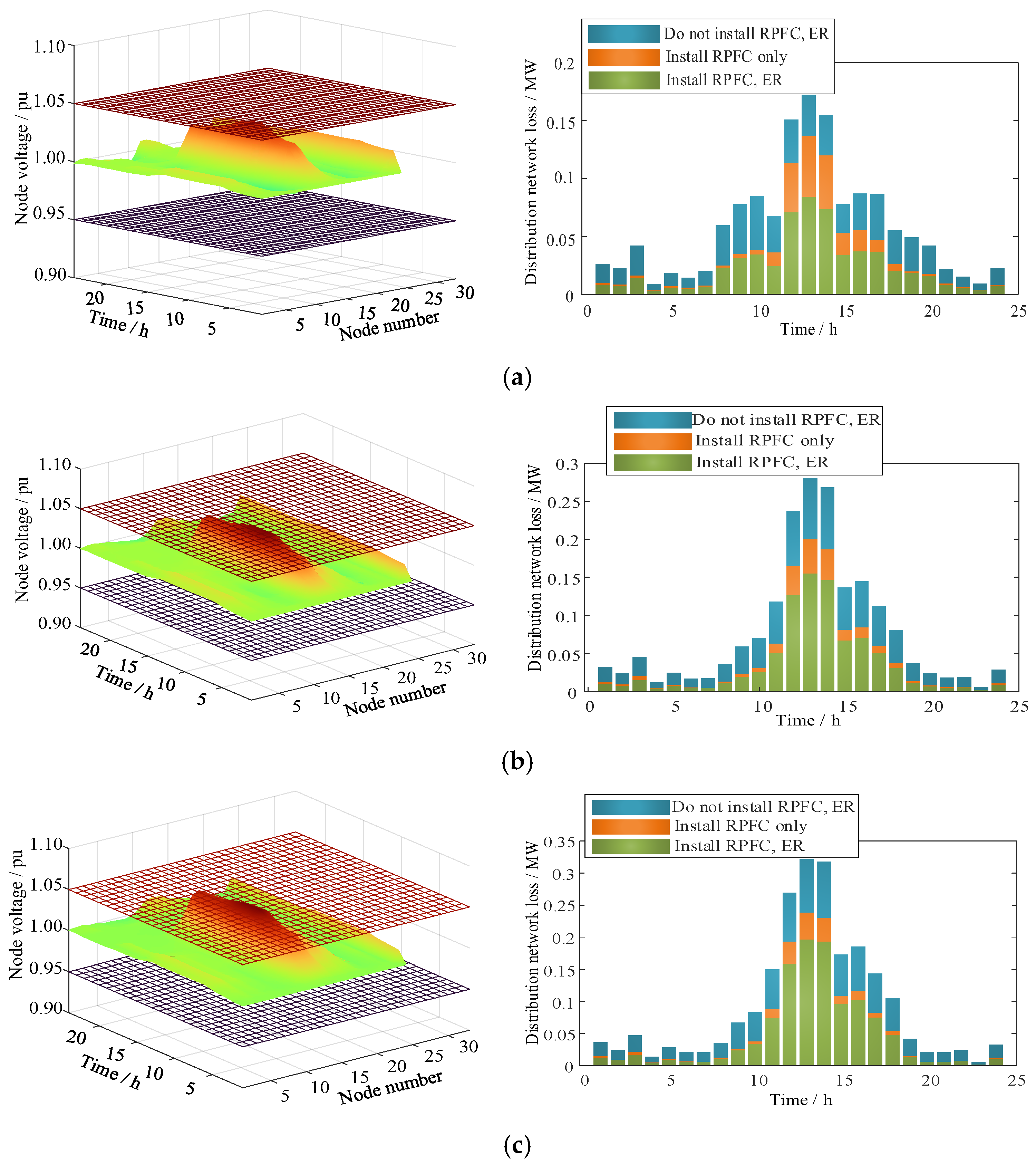
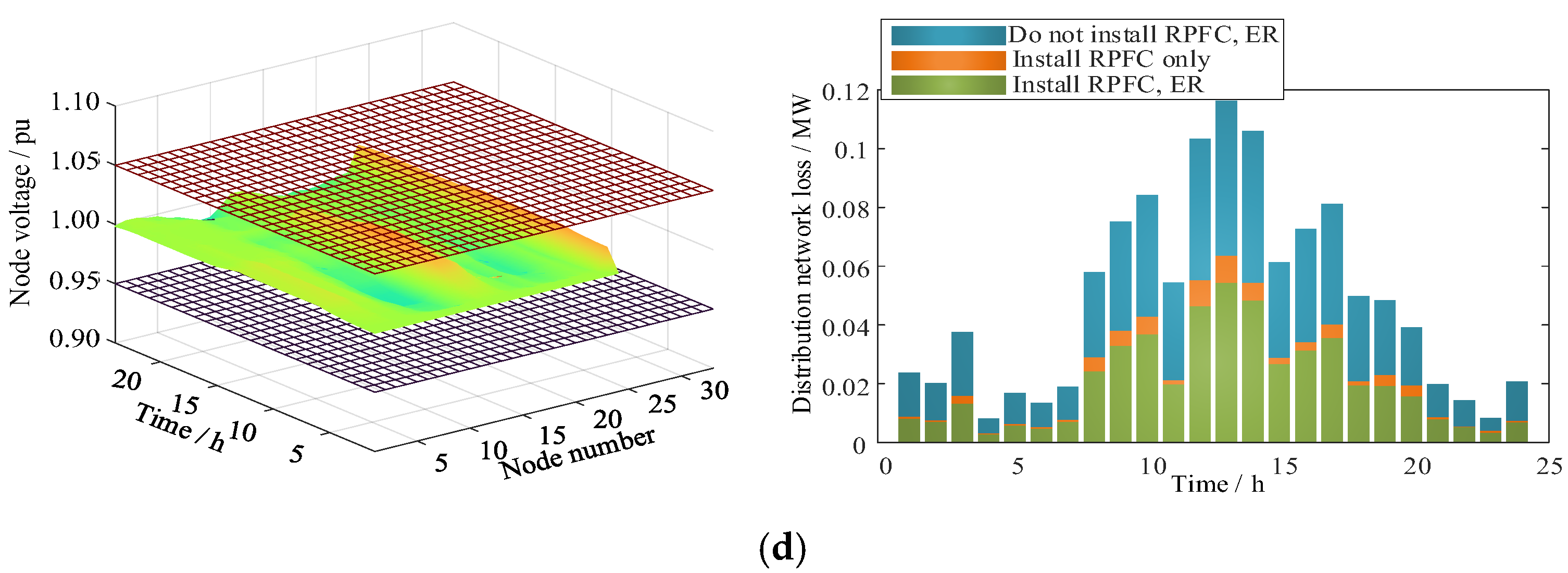
4.1. RPFC and ER Joint Planning Results

To validate the effectiveness of the proposed method, the following comparison scenarios were set up:

Scenario 1: Neither RPFC nor ER is installed. In this case, across several typical daily scenarios, high levels of distributed photovoltaic (PV) integration result in voltage limit violations within the distribution network, as shown in Figure 7.

Scenario 2: Only RPFC is installed. Compared to Scenario 1, the inclusion of RPFC helps mitigate voltage limit violations to some extent and effectively reduces line losses, as illustrated in Figure 8.

Scenario 3: Both RPFC and ER are installed. In contrast to Scenario 2, the combined installation of RPFC and ER addresses voltage and line loss issues from both spatial and temporal dimensions, further reducing voltage deviations and line losses, as demonstrated in Figure 9.

The annual operating costs of the different scenarios are shown in

Table 2. RPFC and ER planning results.

		Option 1	Option 2	Option 3
Decision variables	RPFC	-	(9, 15), (0.8 WM)	(25, 29), (0.5 WM)
	ER	-	-	(15), (0.3 WM)
F1/$	qRPFCFRPFC	-	4290	3431
	qERFER	-	-	2574
F2/$	FO-RPFC	-	7071	3247
	FO-ER	-	-	2480
	Fcur	43,458	-	-
	Floss	41,248	23,426	19,203
Total cost/$		84,706	34,788	30,937

. Since more wind and light rejection exists under the operation of Scenario 1, Scenarios 2 and 3 not only reduce the voltage deviation and the size of the line loss by introducing RPFC and ER, but also reduce the operating cost of its equivalent annual value compared to Scenario 1.

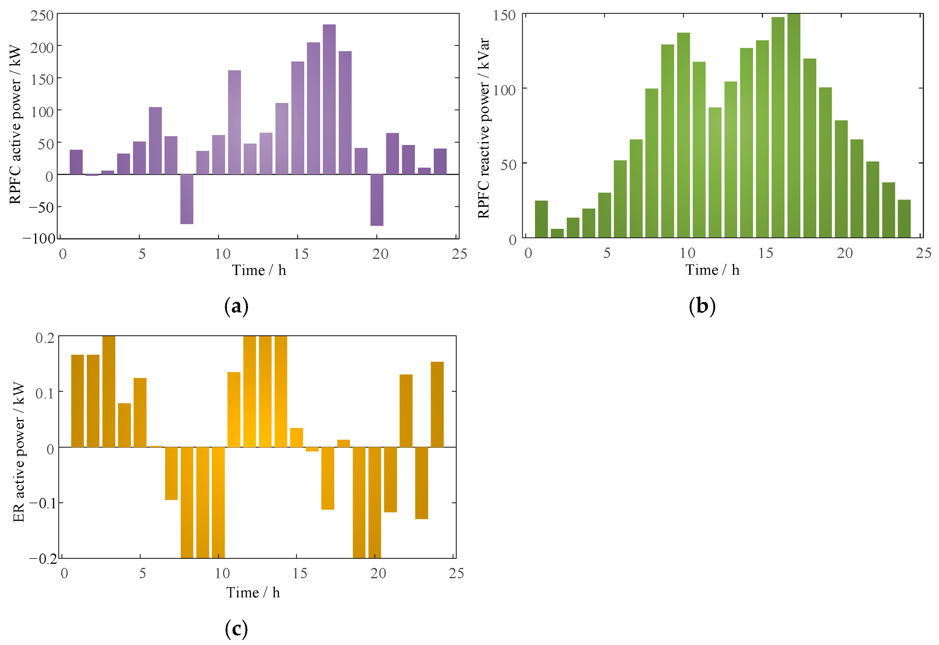
4.2. Analysis of RPFC and ER Response Results

The optimization process is analyzed using Typical Day 1 as an example. Figure 10 shows the time-series graph of active and reactive power at the RPFC ports in Scheme 2. As seen in Figure 5, Figure 6, Figure 7, Figure 8, Figure 9 and Figure 10, during periods of high photovoltaic generation, power support between Node 9 and Node 15 reduces the power transmission path within the IEEE 33-bus system, effectively lowering system operating losses and voltage deviation.

As shown in Figure 11 for the optimization and regulation results of Scheme 3, it can be seen that at the moment of large PV output, in addition to the RPFC participating in the power mutualization at nodes 25 and 29, the ER participates in the energy management at node 15 on the time scale, which further reduces the system network loss.

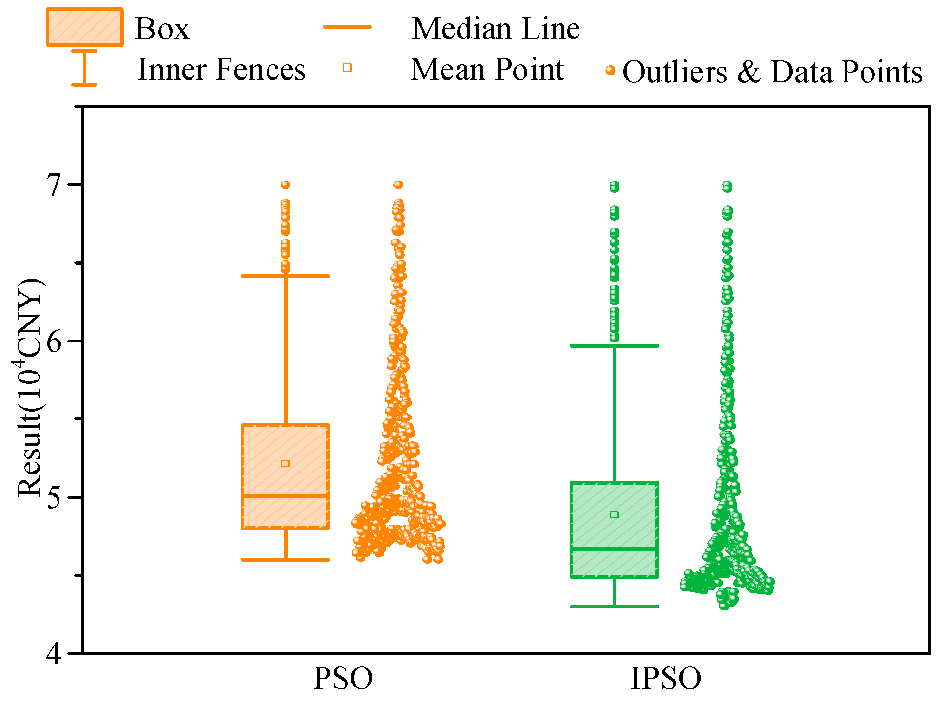
4.3. Algorithm Performance Comparison

The classic Particle Swarm Optimization (PSO) algorithm was compared with the proposed improved PSO algorithm for location planning in Scenario 3. As shown in Figure 12, the convergence curves of the two algorithms reveal a distinct difference: the classic PSO algorithm converges at a value of 46,000, indicating a limited capacity for further exploration in a larger solution space and resulting in a restriction to local optima. In contrast, the convergence curve of the improved PSO algorithm demonstrates a stronger global optimization capability, converging to a significantly lower value. This result indicates that the time-varying parameter enhancements in the improved PSO algorithm enable it to more effectively escape local optima and accelerate convergence.

Figure 13 shows a box plot comparison of the optimization results for the two algorithms. It can be observed that, compared to PSO, IPSO demonstrates a wider exploration range and performs local optimization around the optimal solution, enhancing both global and local optimization capabilities. In contrast, PSO expends significant computation on the local optimum without successfully escaping it.

5. Conclusions

This paper presents an expansion planning method for active distribution networks (ADN) based on the spatiotemporal regulation characteristics of RPFC and ER, with validation through case studies on the IEEE 33-bus system. The main conclusions are as follows:

(1)

The study establishes a two-stage expansion planning model for ADN, incorporating RPFC and ER, and develops a hybrid algorithm based on IPSO and SOCP. This approach optimizes the flexible interconnection of RPFC and ER within a typical distribution network and reduces system line loss costs.

(2)

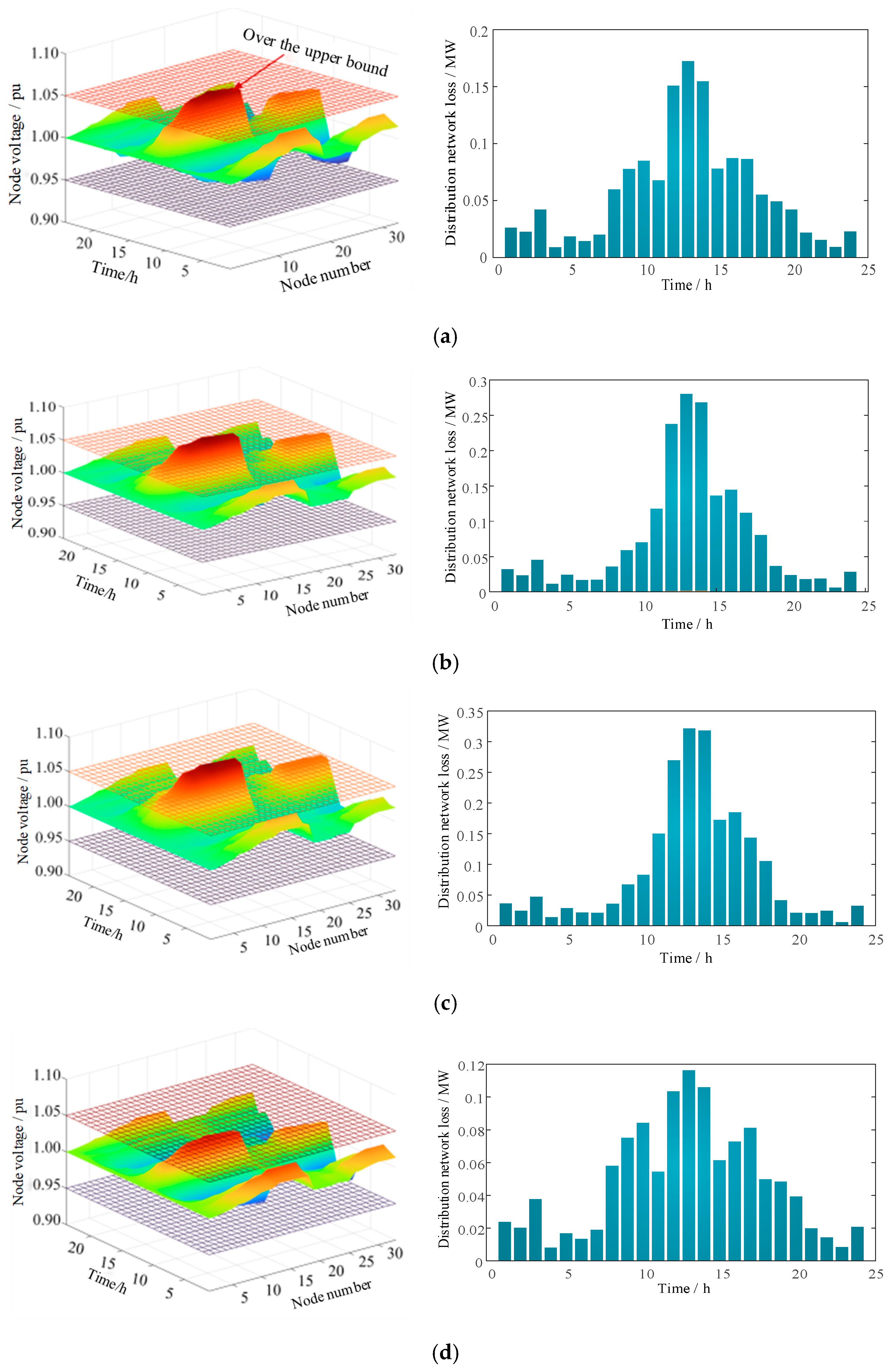
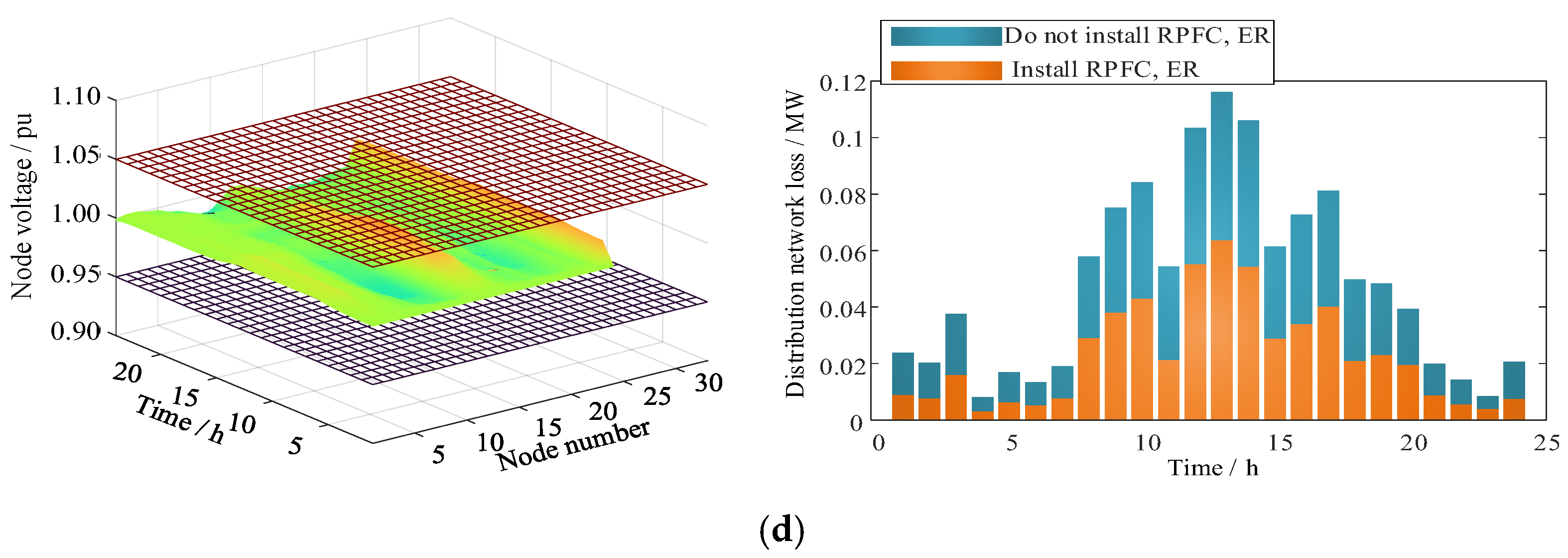
RPFC and ER effectively redistribute power across spatial and temporal dimensions. By appropriately configuring capacities and connection points, they significantly mitigate voltage limit violations at distribution network nodes and reduce line losses.

(3)

Current heuristic-based improvement strategies are limited by computational speed, allowing only for siting and capacity planning of devices like RPFC and ER. These strategies fall short of meeting real-time, minute-level optimization and dispatch requirements. Future research should focus on artificial intelligence techniques to enable rapid scheduling and control of flexible devices.

References

1. Omri, M.; Jooshaki, M.; Abbaspour, A.; Fotuhi-Firuzabad, M. Modeling Microgrids for Analytical Distribution System Reliability Evaluation. IEEE Trans. Power Syst. 2024, 39, 6319–6331. [Google Scholar] [CrossRef]
2. Zhu, W.; Pan, B.; Liu, Q.; Wang, Y.; Shi, D. An accounting method of REDD reduction of renewable energy based on power flow distribution matrix. Int. J. Environ. Technol. Manag. 2024, 27, 232–241. [Google Scholar] [CrossRef]
3. Yan, X.; Peng, W.; Shao, C.; Jia, J.; Li, T. User-Side Voltage Regulation Method Based on Rotary Power Flow Controller. Diangong Jishu Xuebao/Trans. China Electrotech. Soc. 2023, 38, 70–79. [Google Scholar] [CrossRef]
4. Nie, Y.; Nasr Esfahani, M.; Hu, Y.; Li, X.; Alkahtani, M. Multi-Port Energy Router in Mobile Energy Storage for Emergency Power Outage in Urban Cities. Energies 2024, 17, 2927. [Google Scholar] [CrossRef]
5. Li, Z.; He, J.; Wang, X.; Yip, T.; Luo, G. Active control of power flow in distribution network using flexible tie switches. In Proceedings of the 2014 International Conference on Power System Technology, Chengdu, China, 20–22 October 2014; pp. 1224–1229. [Google Scholar] [CrossRef]
6. Solat, S.; Aminifar, F.; Safdarian, A.; Shayanfar, H. An expansion planning model for strategic visioning of active distribution network in the presence of local electricity market. IET Gener. Transm. Distrib. 2023, 17, 5410–5429. [Google Scholar] [CrossRef]
7. Shao, C.; Yan, X.; Yang, Y.; Aslam, W.; Jia, J.; Li, J. Multiple-Zone Synchronous Voltage Regulation and Loss Reduction Optimization of Distribution Networks Based on a Dual Rotary Phase-Shifting Transformer. Sustainability 2024, 16, 1029. [Google Scholar] [CrossRef]
8. Yang, L.; Li, Y.; Zhang, Y.; Xie, Z.; Chen, J.; Qu, Y. Optimal allocation strategy of SOP in flexible interconnected distribution network oriented high proportion renewable energy distribution generation. Energy Rep. 2024, 11, 6048–6056. [Google Scholar] [CrossRef]
9. Chen, Y.; Yang, G.; Song, Z.; Sun, M.; Zhou, S. Optimal configuration method of soft open point considering flexibility of distribution system. In Proceedings of the 2022 IEEE 5th International Conference on Automation, Electronics and Electrical Engineering (AUTEEE), Shenyang, China, 18–20 November 2022; pp. 524–529. [Google Scholar] [CrossRef]
10. Bai, H. An optimization method for operational efficiency of ADN with four-port SSOP. Energy Rep. 2022, 8, 472–479. [Google Scholar] [CrossRef]
11. Yan, X.; Wang, Q.; Bu, J. High Penetration PV Active Distribution Network Power Flow Optimization and Loss Reduction Based on Flexible Interconnection Technology. SSRN, 2023; preprint. [Google Scholar] [CrossRef]
12. Xie, H.; Wang, W.; Wang, W.; Tian, L. Optimal Dispatching Strategy of Active Distribution Network for Promoting Local Consumption of Renewable Energy. Front. Energy Res. 2022, 10, 826141. [Google Scholar] [CrossRef]
13. Xia, S.; Wang, Z.; Gao, X.; Li, W. Optimal planning of mobile energy storage in active distribution network. IET Smart Grid 2024, 7, 1–12. [Google Scholar] [CrossRef]
14. Liu, X. Energy station and distribution network collaborative planning of integrated energy system based on operation optimization and demand response. Int. J. Energy Res. 2020, 44, 4888–4909. [Google Scholar] [CrossRef]
15. Kumar, N.; Kumar, T.; Nema, S.; Thakur, T. A multiobjective planning framework for EV charging stations assisted by solar photovoltaic and battery energy storage system in coupled power and transportation network. Int. J. Energy Res. 2022, 46, 4462–4493. [Google Scholar] [CrossRef]
16. Wang, X.; Guo, Q.; Tu, C.; Li, J.; Xiao, F.; Wan, D. A two-stage optimal strategy for flexible interconnection distribution network considering the loss characteristic of key equipment. Int. J. Electr. Power Energy Syst. 2023, 152, 109232. [Google Scholar] [CrossRef]
17. Rediske, G.; Siluk JC, M.; Gastaldo, N.G.; Rigo, P.D.; Rosa, C.B. Determinant factors in site selection for photovoltaic projects: A systematic review. Int. J. Energy Res. 2019, 43, 1689–1701. [Google Scholar] [CrossRef]
18. Jia, Y.; Li, Q.; Liao, X.; Liu, L.; Wu, J. Research on the Access Planning of SOP and ESS in Distribution Network Based on SOCP-SSGA. Processes 2023, 11, 1844. [Google Scholar] [CrossRef]
19. Wang, J.; Wang, W.; Wang, H.; Wang, S.; Du, J. Two-stage coordinated planning of DG, SOP and ESS in an active distribution network considering violation risk. Dianli Xitong Baohu Yu Kongzhi/Power Syst. Prot. Control 2022, 50, 71–82. [Google Scholar] [CrossRef]
20. Wang, Y.; Wang, X.; Li, S.; Ma, X.; Chen, Y.; Liu, S. Optimization model for harmonic mitigation based on PV-ESS collaboration in small distribution systems. Appl. Energy 2024, 356, 122410. [Google Scholar] [CrossRef]
21. Lee, J.-G.; Jung, S.; Choi, J.-H.; Kim, Y.-H.; Yoon, Y.-B. A study on Energy Storage System (ESS) application for dynamic stability improvement and generation constraint reduction. Trans. Korean Inst. Electr. Eng. 2017, 66, 1554–1560. [Google Scholar] [CrossRef]
Figure 1. ADN expansion planning scheme considering RPFC and ER accesses.
Energies 17 05919 g001
Figure 2. Framework of the RPFC and ER two-tier coordinated planning models.
Energies 17 05919 g002
Figure 3. Solving two-layer planning model based on IPSO and SOCP.
Energies 17 05919 g003
Figure 4. Classical particle swarm algorithm movement.
Energies 17 05919 g004
Figure 5. Flowchart for solving the bilayer model.
Energies 17 05919 g005
Figure 6. IEEE33 node active distribution network with DGs.
Energies 17 05919 g006
Figure 7. Distribution network voltage and line loss without RPFC and ER participation. (a) Typical day 1; (b) Typical day 2; (c) Typical day 3; (d) Typical day 4.
Energies 17 05919 g007
Figure 8. Voltage and line loss of the distribution network with only RPFC installed. (a) Typical day 1; (b) Typical day 2; (c) Typical day 3; (d) Typical day4.
Energies 17 05919 g008aEnergies 17 05919 g008b
Figure 9. Voltage and line loss of the distribution network with RPFC and ER installed together. (a) Typical day 1; (b) Typical day 2; (c) Typical day 3; (d) Typical day 4.
Energies 17 05919 g009aEnergies 17 05919 g009b
Figure 10. RPFC operation regulation under optimized regulation strategy. (a) Interconnection node active power; (b) Interconnection node reactive power.
Energies 17 05919 g010
Figure 11. RPFC and ER operation under optimized regulation strategy. (a) Interconnection node active power; (b) Interconnection node reactive power; (c) Power exchange at ER access nodes.
Energies 17 05919 g011
Figure 12. Comparison of Algorithm Convergence Curves.
Energies 17 05919 g012
Figure 13. Comparison of Algorithm Box Plots.
Energies 17 05919 g013