Article

Non-Condensation Turbulence Models with Different Near-Wall Treatments and Solvers Comparative Research for Three-Dimensional Steam Ejectors

1
Zhan Tianyou College, Dalian Jiaotong University, Dalian 116028, China
2
Bingshan Refrigeration & Heat Transfer Technologies Co., Ltd., Dalian 116630, China
3
Department of Thermal Energy and Power Engineering, Yantai University, Yantai 264005, China
4
School of Energy and Power Engineering, Dalian University of Technology, Dalian 116024, China
*
Author to whom correspondence should be addressed.
Energies 2024, 17(22), 5586; https://doi.org/10.3390/en17225586
Submission received: 14 October 2024 / Revised: 5 November 2024 / Accepted: 6 November 2024 / Published: 8 November 2024

Abstract

:
Steam ejectors are important energy-saving equipment for solar thermal energy storage; however, a numerical simulation research method has not been agreed upon. This study contributes to a comprehensive selection of turbulence models, near-wall treatments, geometrical modeling (2-D and 3-D), solvers, and models (condensation and ideal-gas) in the RANS equations approach for steam ejectors through validation with experiments globally and locally. The turbulence models studied are k-ε Standard, k-ε RNG, k-ε Realizable, k-ω Standard, k-ω SST, Transition SST, and linear Reynolds Stress. The near-wall treatments assessed are Standard Wall Functions, Non-equilibrium Wall Functions, and Enhanced Wall Treatment. The solvers compared are pressure-based and density-based solvers. The root causes of their distinctions in terms of simulation results, applicable conditions, convergence, and computational cost are explained and compared. The complex phenomena involving shock waves, choking, and vapor condensation captured by different models are discussed. The internal connections of their performance and flow phenomena are analyzed from the mechanism perspective. The originality of this study is that both condensation and 3-D asymmetric effects on the simulation results are considered. The results indicate that the k-ω SST non-equilibrium condensation model coupling the low-Re boundary conditions has the most accurate prediction results, best convergence, and fit for the widest range of working conditions. A 3-D asymmetric condensation model with a density-based solver is recommended for simulating steam ejectors accurately.

1. Introduction

Steam ejectors are important and widely used energy-saving equipment that can only utilize residual pressure by recovering low-pressure steam [1]. Although a steam ejector’s structure is simple and reliable, the flow and mixing process of its internal fluid is very complicated [2]. Many kinds of flow phenomena that affect the ejector performance occur in the flow field, such as shock waves [3], choking [4], and condensation [5]. These flow phenomena cause the transonic phase transition and the sudden change of various flow parameters in the flow field. It is difficult to obtain accurate measurements in supersonic fluids by current experimental methods. Computational fluid dynamics can quantitatively describe the complex flow phenomena that make up for the shortage of experiments. Assessment of these dynamics is an effective method to study the relationship between flow phenomenon and ejector performance. Therefore, the method of simulated steam ejectors to get accurate results is worth investigating.
The RANS (Reynolds-Averaged Navier–Stokes) equations are the most frequently used equations in scientific research and engineering practice simulations. According to the different closures, the turbulence models of the RANS equations are divided into two categories: the Reynolds Stress Model and eddy-viscosity closures. The eddy-viscosity closures include the zero-, one-, and two-equation turbulence models [6]. Among these, the two-equation turbulence models that include the k-ε series and k-ω series models are adopted in ejector simulations.
The turbulence models’ closures of the RANS equations in simulating ejectors have not reached a consensus [7,8]. For air ejectors, Hemidi et al. [9] compared two turbulence models. They observed that both k-ε Standard and k-ω SST predicted almost the same Er (entrainment ratio) but had completely different local flow characteristics under higher working pressures. Overall, the k-ε Standard is better. Gagan et al. [10] compared six turbulence models (k-ε series, k-ω series, and RSM) of flow visualization using the PIV technique. The supersonic flow shape and the subsonic region velocity are best obtained by the k-ε Standard. For N2 ejectors, Zhu and Jiang [11] compared four turbulence models (k-ε series, k-ω SST) based on visualization experiments. They stated that the shock train configuration obtained by the k-ε RNG accorded best with the experimental data. For R134a ejectors, Croquer et al. [12] compared four turbulence models (k-ε series, k-ω SST) with the ideal-gas equation and real-gas equation. They found the k-ω SST obtains accurate Er only when the real-gas equation is used. For steam ejectors, scholars neglect condensation effects during the comparison of turbulence models. Ruangtrakoon [13] and Besagni [8] both recommended the k-ω SST. The former compared two models (k-ε Realizable, k-ω SST), and the latter compared seven models (k-ε Standard, k-ε RNG, k-ε Realizable k-ω standard, k-ω SST, Spalart-Allmaras, and RSM). Han et al. [14] and Varga et al. [15] obtained different comparison results. Han et al. [14] compared four models (k-ε series, k-ω SST) and stated that the pressure distribution of the k-ε Realizable model accorded best with experiments. Varga et al. [15] compared six models (k-ε series, k-ω series, Transition SST) and stated that the ejector performance of the Transition SST accorded best with experiments. However, they assumed that water vapor was an ideal gas and ignored condensation.
Apart from turbulence models, near-wall treatments should be cautiously adopted. Two commonly used near-wall treatments are the wall function and near-wall modeling. The former is to resolve the viscosity-influenced region by wall functions containing semi-empirical formulas, and its turbulence models do not require modification. The RSM and the k-ε series models need wall functions that include Standard Wall Function (SWF), Non-equilibrium Wall Function (NWF), Enhanced Wall Treatment (EWT), and so on. The latter approach is to modify the turbulence model so that the region affected by viscosity can be analyzed by a fine near-wall mesh. As to the comparative study of near-wall treatments, Besagni et al. [8] stated that EWT allows achieving generally better results than SWF and NWF, and nearly no differences between the SWF and EWT results. Han et al. [14] compared SWF and EWT for the prediction of a steam ejector. They found that the latter was superior to the former. Wu et al. [16,17] considered the effect of fluid–structure interaction. However, no agreement about near-wall treatments has been reached.
According to the classical viewpoint, flow fields with shock waves must adopt the density-based solver(D-B) owing to its excellent adaptability of the simulation for compressible and super-sonic flows [18]. However, the pressure-based solver (P-B) is for low-speed incompressible flow, historically [11]. Nevertheless, in the works of Li and Li [19], Yazdani et al. [20], Croquer et al. [12], Sriveerakul et al. [21], Besagni et al. [7], and Bourhan et al. [22], the pressure-based solver was proposed to solve supersonic problems in ejectors. Therefore, a comparative study of the two solvers is a great lack that at present needs to be performed on steam ejectors.
The ideal-gas model is adopted in related comparative research on steam ejectors. Nevertheless, the flow information and performance of steam ejectors are both affected by non-equilibrium condensation [23]. Moreover, most scholars simplify steam ejectors into a 2-D axisymmetric model in simulations to save calculation costs, ignoring the 3-D disturbance in actual flow fields. Mazzelli et al. [24] compared the prediction of ejector coefficients by 2-D and 3-D standard k-ε, Realizable k-ε, SST k-ω, and RSM models. Results showed that only the simulation results of the 3-D model are in the reliable range under the sub-critical operating state. Therefore, the comparative research of the turbulence models with different near-wall treatments and solvers should consider both condensation effects and 3-D effects, which the current research lacks.
Consequently, a study that contributes to a comprehensive selection of turbulence models, near-wall treatments, geometrical modeling (2-D and 3-D), solvers, and models (condensation and ideal-gas) in the RANS equations approach for steam ejectors is urgently needed. In this article, a condensation model with seven turbulence models (k-ε series, k-ω series, Transition SST, linear Reynolds Stress Model), three near-wall treatments (SWF, NWF, EWT), and two solvers (D-B and P-B) is utilized to simulate different sizes of 3-D steam ejectors under variable working conditions. The root causes of their distinctions in simulation results, applicable conditions, convergence, and computational cost are explained and compared. The complex phenomena involving shock waves, choking, and vapor condensation captured by different models are discussed. The connections between the ejector performance and local flow phenomena are analyzed. The originality of the study is that both condensation and 3-D asymmetric effects on the simulation results are considered. These research achievements provide rational foundations for simulation research of steam ejectors.

2. Numerical Simulation Method

2.1. Mathematical Model

Below are three conservation equations of wet steam at steady state:
x j ρ v j = 0
x j ρ v j v i = τ i j x j P x i
x j v j ρ E + P = x j λ e f f T x j + x j v i τ i j
where E is the total energy contained in the fluid per unit mass (equal to the sum of the specific internal energy and kinetic energy):
E = h p ρ + 1 2 v j v j
The real state of vapor is expressed by [25]:
P = ρ v R T 1 + B ρ v + C ρ v 2
where B and C are the virial coefficients which are detailed in the reference [25].
The vapor properties, equations of saturated vapor and saturated liquid lines, and liquid properties are detailed in the references [26]. The wet steam density and the properties φm of wet steam are:
ρ = ρ v / 1 β
φ m = φ l β + 1 β ψ v
where β is the liquid mass fraction which is equal to the ratio of the mass of the condensate to the total mass.
Mach number is an important dimensionless number for determining sonic velocity flow. It is equal to the ratio of fluid speed to sonic velocity:
M a = v / a
where a is the sonic velocity of wet steam [27]:
a = ρ β ρ v a v 2 + 1 β ρ l a l 2 1 / 2
The governing equations for vapor–liquid two-phase mixtures are established based on the Euler coordinate system [28]:
ρ v β = Γ
ρ v η = ρ J
where Γ is the liquid mass generation rate that is composed of a two-part mass increase: the first term of the right end equation shows the mass of the liquid phase generated by spontaneous nucleation, and the second term shows the mass of the liquid phase generated by the droplet growth after nucleation [28]; J is nucleation rate [29]; and η is the number of droplets per unit volume:
Γ = m ˙ l = m ˙ v = 4 3 π ρ l J r * 3 + 4 π ρ l η r ¯ 2 r ¯ t
J = q c 1 + θ ρ g 2 ρ l 2 σ M m 3 π e 4 π r * 2 σ 3 k B T g
η = β 1 β V d ρ l / ρ g
V d = 4 3 π r ¯ 3
where Vd is a mean droplet volume, and the average droplet radius is from Vd and η:
r ¯ = 3 β 4 π η ( 1 β ) ( ρ l ρ g ) 3
The droplet’s growth rate equation [29] is:
r ¯ t = P h lv ρ l 2 π R T γ + 1 2 γ C l 1 r * r ¯ Δ T
where hlv is the specific latent enthalpy and the ΔT is the degree of subcooling which is equal to:
Δ T = T sat T

2.2. Solution Scheme and Boundary Conditions

The finite-volume method was used to treat N-S equations at a steady state with the 7 turbulent models respectively based on Fluent. The implicit solver was based on density coupling. The variable gradient interpolation method was the Green–Gauss method based on node. The second-order upwind scheme was utilized. It is convergent when it meets the following 3 criteria:
(1)
All the residual terms’ convergence absolute criteria are <10−6 forever;
(2)
The difference in the mass flow rate between the inlet and the outlet is <1 × 10⁻⁷;
(3)
The calculated mass flow rate of two inlet sections and one outlet section is stable.
Figure 1 describes the ejector sizes and Table 1 illustrates the working conditions, using data from Chen and Sun’s experiment [30]. The variables Pm and Tm represent the temperature and pressure of the motive fluid, while Ps and Ts denote the temperature and pressure of the suction fluid. Additionally, Pd signifies the pressure of the discharge fluid. The case labels are consistent with those in the reference. The simulation parameters are consistent with the experimental parameters to compare their results. The computation parameters in Table 1 are given as the boundary conditions for pressure inlet and pressure outlet, given that outlet pressures are constant. The turbulence boundary conditions are set as the turbulence intensity and the turbulent viscosity ratios. For the motive steam and the suction steam, their turbulent viscosity ratios are 500 and 100, respectively, and their turbulence intensity are 5.0% and 2.0%, respectively. There is no slip and no penetration in the adiabatic smooth solid walls, hypothetically.

2.3. Mesh Creation

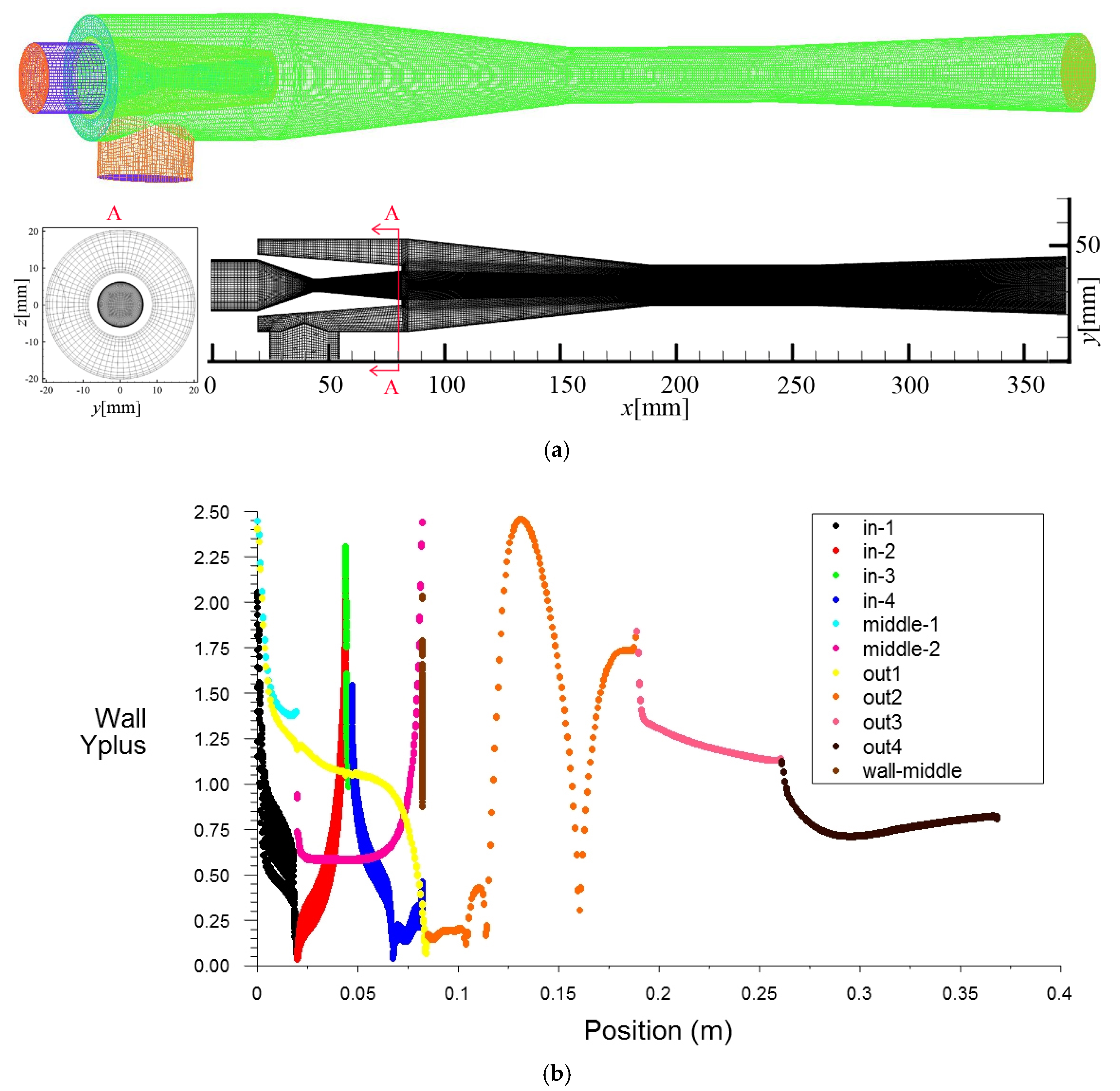
The 3-D meshes of E1 and E2 with refinement both around boundary layers and the shock waves were created. Furthermore, each mesh was divided into two categories according to the y+ value that indicates the dimensionless distance of a first-layer node from the wall. The first mesh type with y+ ≈ 1 was used for EWT, and the second mesh type with y+min > 30 was used for SWF and NWF. The first type of meshes of E2 are shown in Figure 2a and their y+ values along the ejector wall are shown in Figure 2b. Except for the near-wall area, the two meshes have the same structures. The second type of mesh was obtained by locally adjusting mesh density around the near-wall area of the first type.
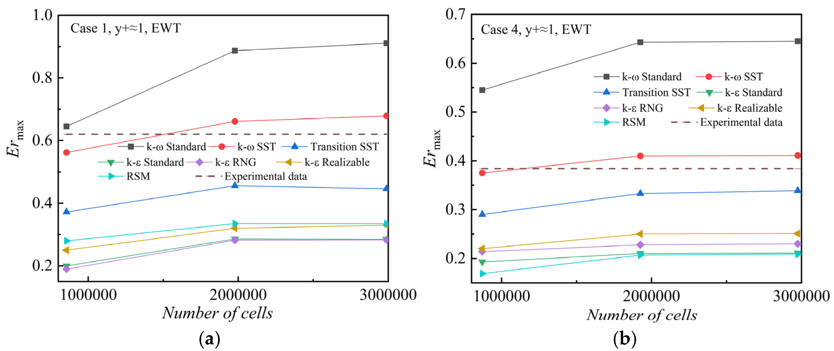
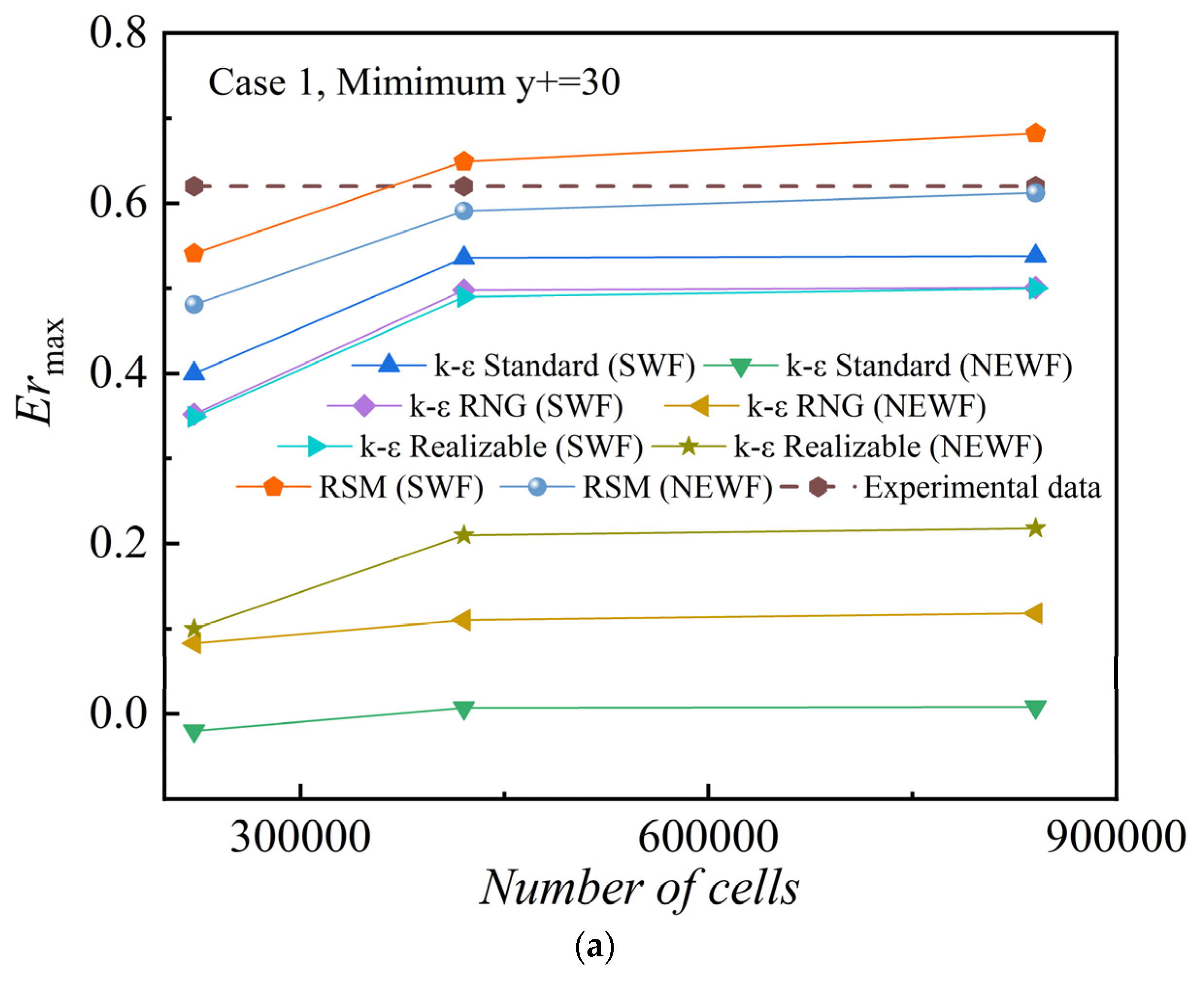
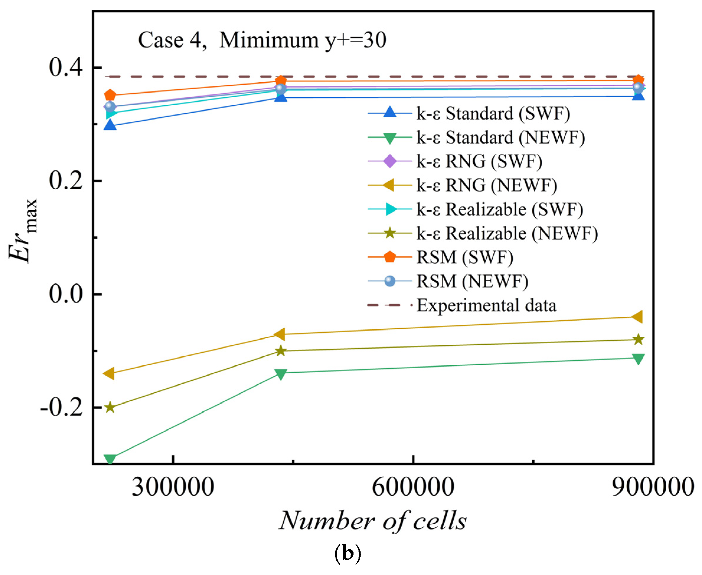
Table 2 summarizes the number of cells of the two-type grids. Figure 3 and Figure 4 illustrate that the ejection coefficients obtained by medium-level grids are similar to those of the fine-level grids when all other things are equal. Moreover, the time cost and the computation cost of the medium-level grids are lower than those of the fine-level grids. Accordingly, the medium-level grids were adopted in this paper.

3. Results and Discussion

3.1. Validation, Comparison and Analysis of Different Near-Wall Treatments

Turbulent flow is divided into inner and outer layers according to a distance along the near wall. The flow in the outer layer is completely turbulent, and the flow in the inner layer can be affected by the wall obviously. According to the y+ value, the inner layer is divided into three sub-layers: a viscous sublayer (y+ < 5), a buffer layer (5 ≤ y+ ≤ 30), and a log-law region 30 < y+ < f(Re) [6].
The k-ε series and linear RSM require selecting near-wall treatments. The near-wall treatments commonly used for ejectors are SWF, NWF, and EWT. SWF and NWF cannot truly resolve the viscous sublayer and buffer layer, but utilize semi-empirical formulas to bridge the wall and the fully-turbulent region. Therefore, their first node of the near-wall grid must be arranged in the log-law region, namely y+min > 30. The SWF can reasonably predict the bounded flow of most walls with high Reynolds numbers. The NWF can partially consider the influence of pressure gradient, which further expands the applicability. The EWT is suggested when the flow has special conditions, such as severe pressure gradient, boundary layer separation, and so on. This method can analyze the viscous sublayer if the near-wall region has a fine mesh [6]. Therefore, the first node of the near-wall mesh is arranged within the viscous sublayer, namely y+ ≈ 1.
The mathematical structures of the k-ω series and Transition SST already emphasize the near-wall flow. Therefore, there is no need to select any near-wall treatments. Their wall boundary conditions for the k equation are treated likewise as the k equation treated when EWT is applied in k-ε models [6]. When the grid in the near-wall region is very dense (y+ ≈ 1), these three turbulence models coupled with the low-Re boundary conditions can deal with the complex flow.
Figure 3a,b compare the Ermax of experimental data and seven different turbulence models combined with EWT. Results obtained from the k-ω SST are reasonable with an average relative error ( e ) of 7%.
Figure 4a,b compare the Ermax of experimental data and seven turbulence models combined with SWF or NWF. The linear RSM combined with SWF or NWF can reasonably predict the Ermax with e of 1.5% and −5.5%, respectively, whereas the convergence of NEWF is worse than that of SWF, and the steps of iterations that reach the convergent condition are 1.8 times that of SWF.
The Ermax predicted by the EWT or NEWF combined with the k-ε series deviates greatly from the experimental data. Even the Ermax predicted is less than 0, which indicates the reverse flow as shown in Figure 4. The SWF combined with the k-ε series are just suitable for Case 4 with the lowest pressure, and their relative errors are −10%, −5%, and −6% respectively.
Therefore, the near-wall treatment method should be selected according to the specific turbulence model and working conditions. Moreover, it is also affected by the structure of the supersonic steam ejector according to the comparison results of E1 and E2.

3.2. Validation, Comparison and Analysis of Different Turbulence Models

Each Ermax predicted by k-ω SST is within an acceptable range (relative error of −5%~11%) for each case as shown in Figure 5. The Ermax predicted by the linear RSM has only one large deviation (−19%) compared to experimental data. The average relative error ( e ) of Ermax obtained from the k-ω SST and linear RSM which are 4.0% and −5.2%, respectively, are within the acceptable range, as shown in Table 3. Their maximum relative errors are 11% and −19%, respectively. Therefore, the two models may have the potential to provide accurate predictions for steam ejectors.
Compared to the experiments, Ermax predicted by k-ω Standard are greater for all cases with an e of 34.5%. The Ermax of the k-ε Standard, k-ε RNG, k-ε Realizable, and Transition SST have an e of −39.5%, −36.5%, −28.6%, and −30.6%, respectively, compared to experimental values. However, the minimum relative errors, which are −10%, −5%, −6%, and −13%, respectively, obtained by the three models under Case 4 are within the acceptable range. Case 4 has the lowest primary inlet pressure for E2 of all cases. Furthermore, Case 1 has the lowest primary inlet pressure for E1 and also has the lowest relative errors of all E1 cases. Therefore, the simulation accuracy of the three turbulence models has a strong dependence on the motive pressure. It appears that the Ermax can be reasonably predicted by the three models only under relatively low-pressure conditions with the same physical dimensions. Moreover, pressure dependence has a different sensitivity to different structures of ejectors.
The difference in Ermax predicted by different models depends mainly on their mass flow rates of suction steam (Gs) as shown in Table 4. Under the same case, the mass flow rates of motive steam (Gm) predicted by different models are close. The maximum difference is 8% and the minimum difference is 2%. However, Gs predicted by different models are significantly different. The maximum difference is 129% and the minimum difference is 55%. The k-ω Standard predicts the maximum Gs under each case, which causes the overestimation of Ermax.
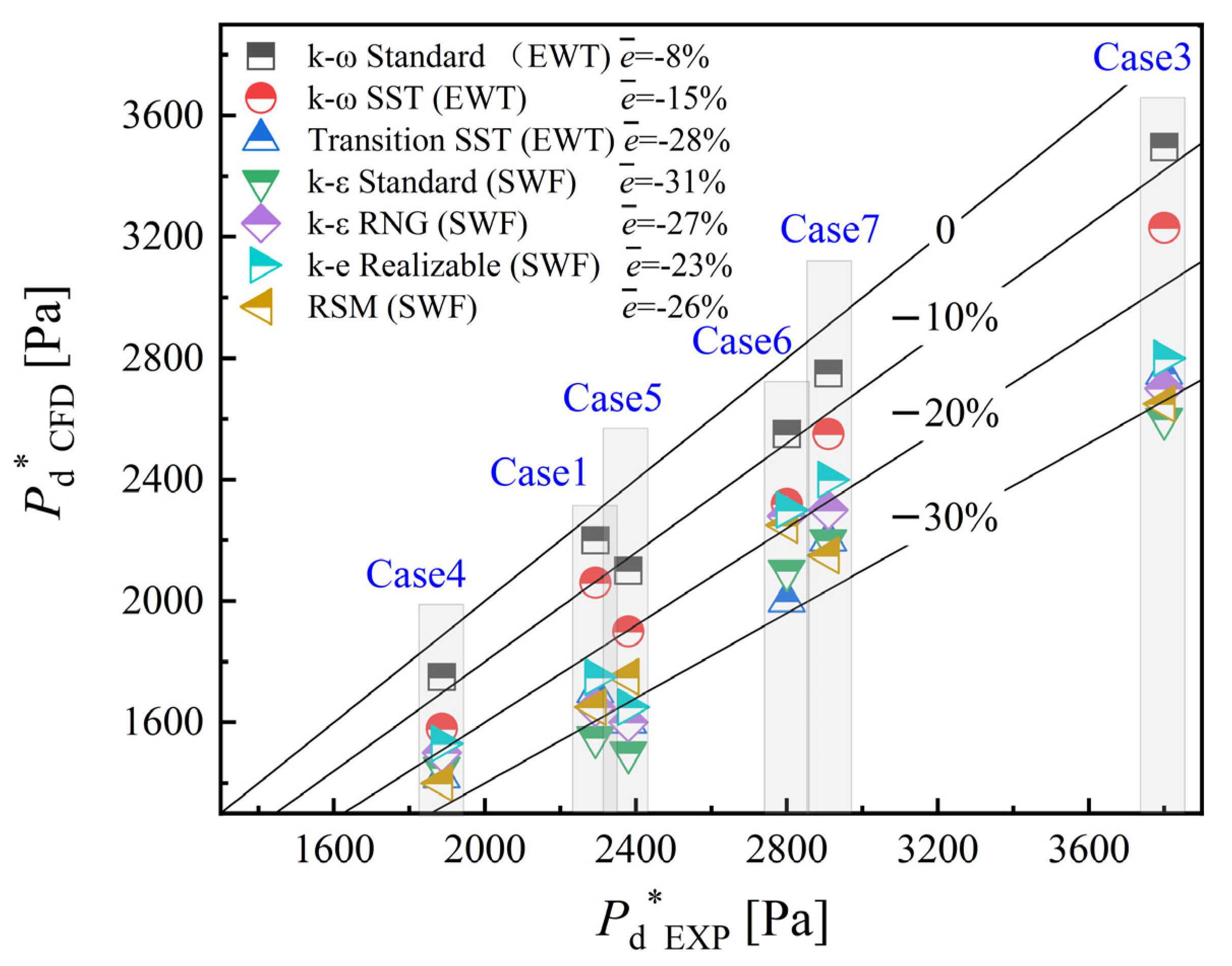
As to the comparison of Pd* by different turbulence models in Figure 6, they are less than the experimental data, which accords with the majority of results [31,32,33,34,35,36]. Since the Pd* for Case 2 and Case 7 is too close to clearly illustrate in Figure 6, Case 2 in Figure 6 is omitted. The e of k-ω Standard and k-ω SST are within an acceptable range, which is −8.0% and −15%, respectively. Although the relative error of Pd* predicted by k-ω Standard is the lowest, the e of Ermax predicted by k-ω Standard is as high as 34.5%. Therefore, as to the ejector performance, k-ω SST agrees with the experimental results.
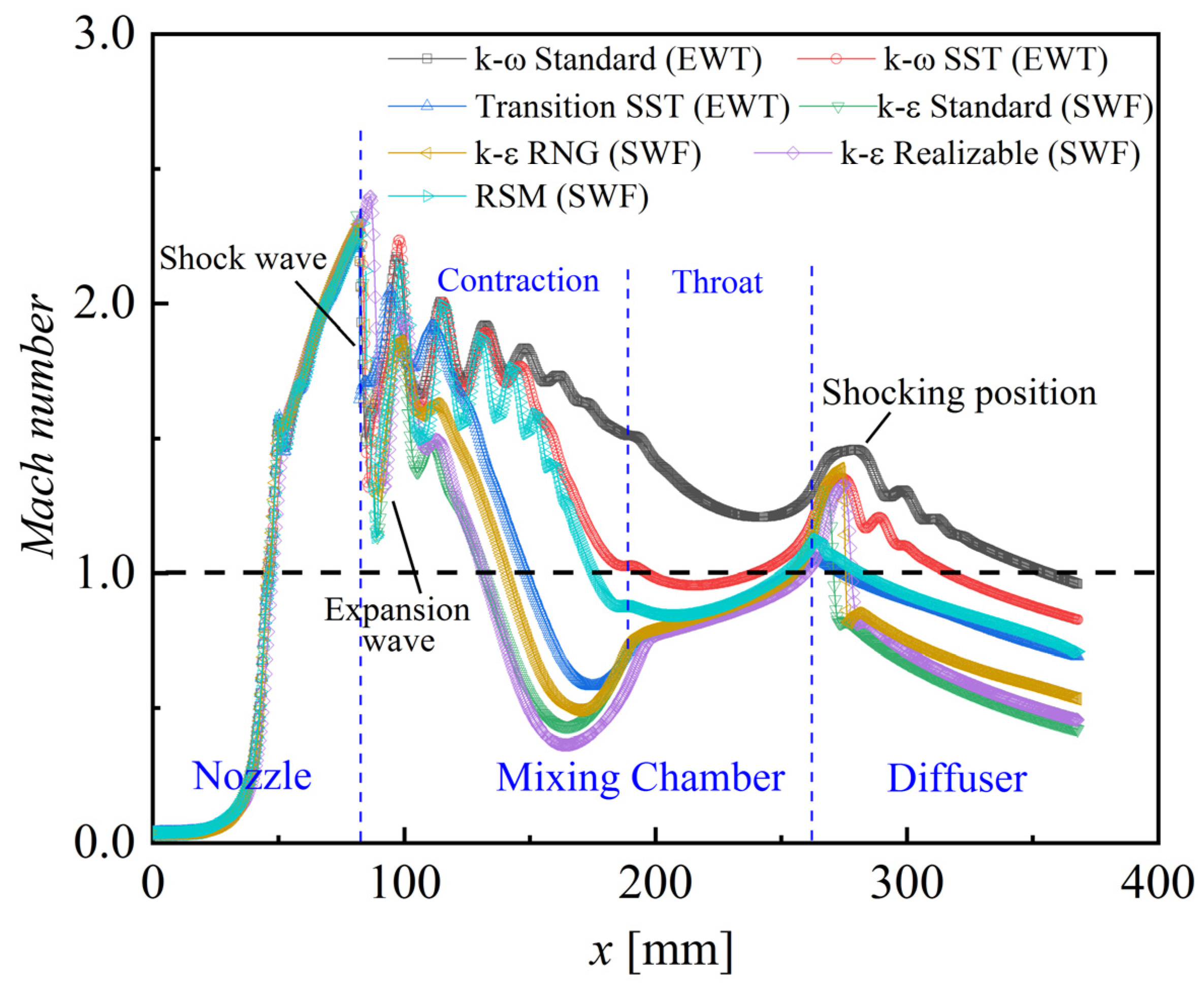
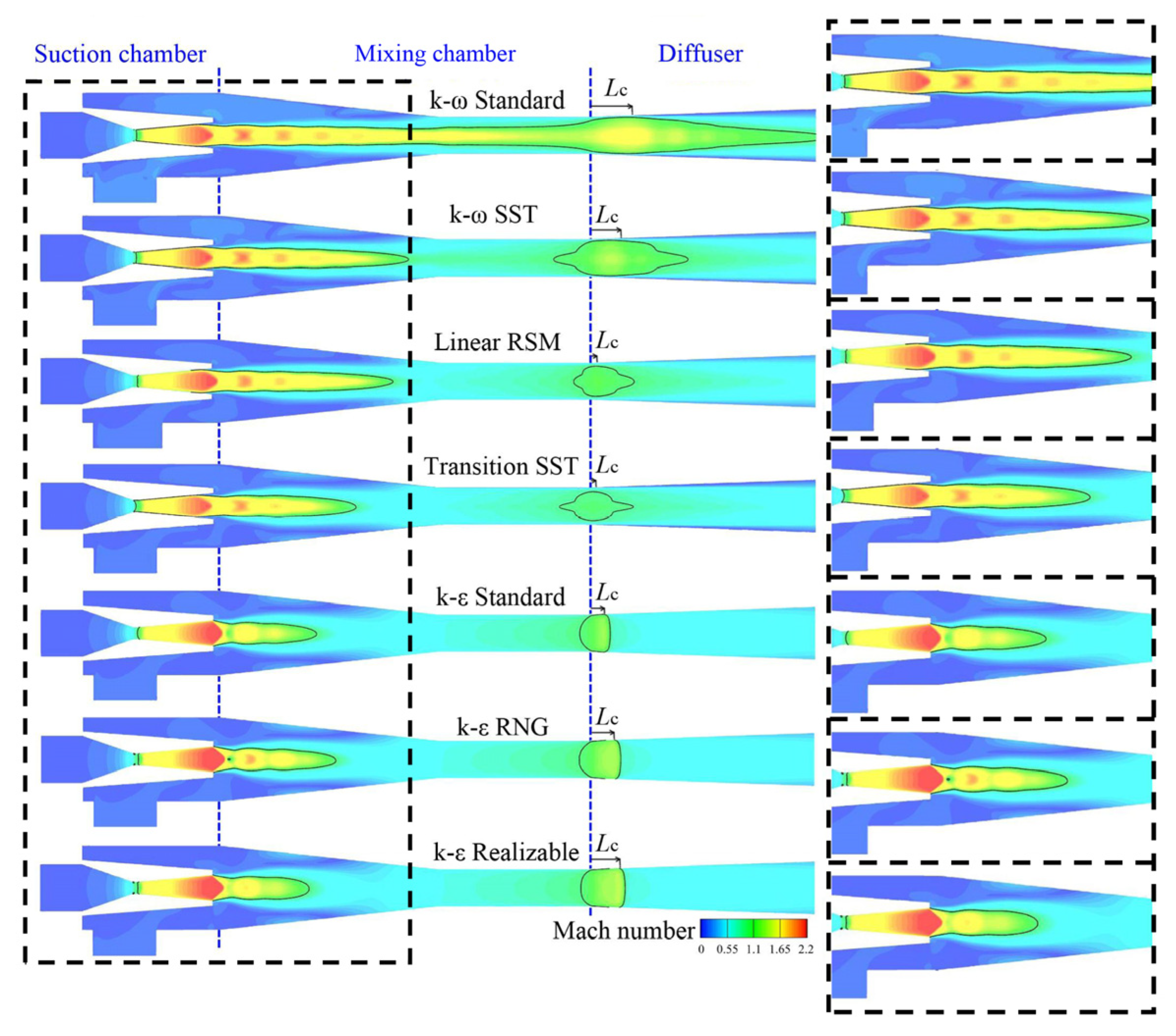
Differences in Pd* are explained through the local flow characteristics of the second choking in Figure 7 and Figure 8. The black outline in Figure 8 is the sonic line whose Mach number is 1. The sonic line at choking mode is closest to the wall [9]. The appearance of the first shock wave in the diffuser reduces the fluid Mach number, causing the sonic line to move away from the wall, and the second choking phenomenon ends. The distance between the first shock wave position and the ejector outlet is positive with the second choking length (Lc). When Lc increases, the differences between Pd and Pd* are getting greater [37]. Accordingly, when the working condition is the same, Pd* predicted by different turbulence models increases with the distance between the first shock wave position and the ejector outlet by comparing Figure 6 and Figure 7. The order of the distances from large to small is the k-ω Standard, k-ω SST, k-ε Realizable, k-ε RNG, k-ε Standard, linear RSM, and Transition SST, as shown in Figure 7. The same order of Pd* is shown in Figure 6.
An abrupt decrease of Ma represents that an aerodynamic shock wave occurs, as shown in Figure 7 and Figure 8. The aerodynamic shock wave whose shock surface is perpendicular to the flow direction and whose flow direction is unchanged after passing through the shock wave is a normal shock wave. Otherwise, it is an oblique shock. Velocity after a normal shock wave must be subsonic. However, velocity after an oblique shock wave is not certain. As can be seen in Figure 7 and Figure 8, the k-ε series models get a normal shock, while the others obtain a series of oblique shock waves that accord with the experiments [30].
In steam ejectors, vapor experiences a transonic expansion process of rapid depressurization and cooling. When the vapor crosses a saturation line, it does not immediately condense due to the free energy barrier. The vapor expands continuously, resulting in the vapor temperature continuing to decrease, and the vapor diverges from the saturation equilibrium state. When the unbalanced state develops to a certain extent, the non-equilibrium condensation phenomenon occurs. Results of the linear RSM, k-ω Standard, k-ω SST, and Transition SST agree with Chen and Sun’s observation [30], as can be seen in Figure 9.
The computational effort mainly depends on the turbulence model utilized when the discretization scheme, grid density, numerical solution method, and boundary conditions are fixed [8]. According to the convergence criteria reported above, taking the 3-D asymmetric mesh of E2 with 2 million elements under Case 8 as an example, the steps of iterations with the same initialization condition for the seven models are used for the computational effort and convergence capability analysis.
As to the comparative study of the computational effort, the k-ε Standard with the least iteration number is taken as a reference. Their relative iteration number is summarized in Table 5. The calculations showed that among the seven turbulence models, the linear RSM model has the highest relative computational cost and is the most difficult to converge. This is due to the fact that it takes into account the anisotropy of turbulent viscosity, which requires an additional seven transport equations in three-dimensional flow, greatly increasing the computational cost and time cost, and weakening the convergence of iterative calculations in some cases, even failing to meet the convergence conditions. The relative computational cost of the transition SST model is only slightly less than that of the linear RSM model, as it has four transport equations. The remaining turbulence models are all two-equation turbulence models, so their relative computational cost is smaller. An item that reflects the time-averaged strain rate of the mainstream is added to the ε equation in the k-ε RNG. A content involving rotation and curvature is added to the k-ε Realizable’s turbulent viscosity equation [6]. Therefore, the iteration number of Standard is the least of the k-ε series.
As to the convergence capability of the seven turbulence models, the reduction in mass or energy residuals is the slowest. The linear RSM is the most difficult model to converge, owing to its high degree of non-linearity. k-ω SST is the easiest to reach convergence, which is aligned with the conclusions of Besagni et al. [8], although the models compared are different.
In summary, considering condensation and 3-D effects, the k-ω SST model with low Reynolds number boundary conditions has the most accurate prediction results globally and locally, the best convergence, a low computational cost, and can be applied to the widest range of working conditions.

3.3. Comparison and Analysis of Density-Based Solver and Pressure-Based Solver

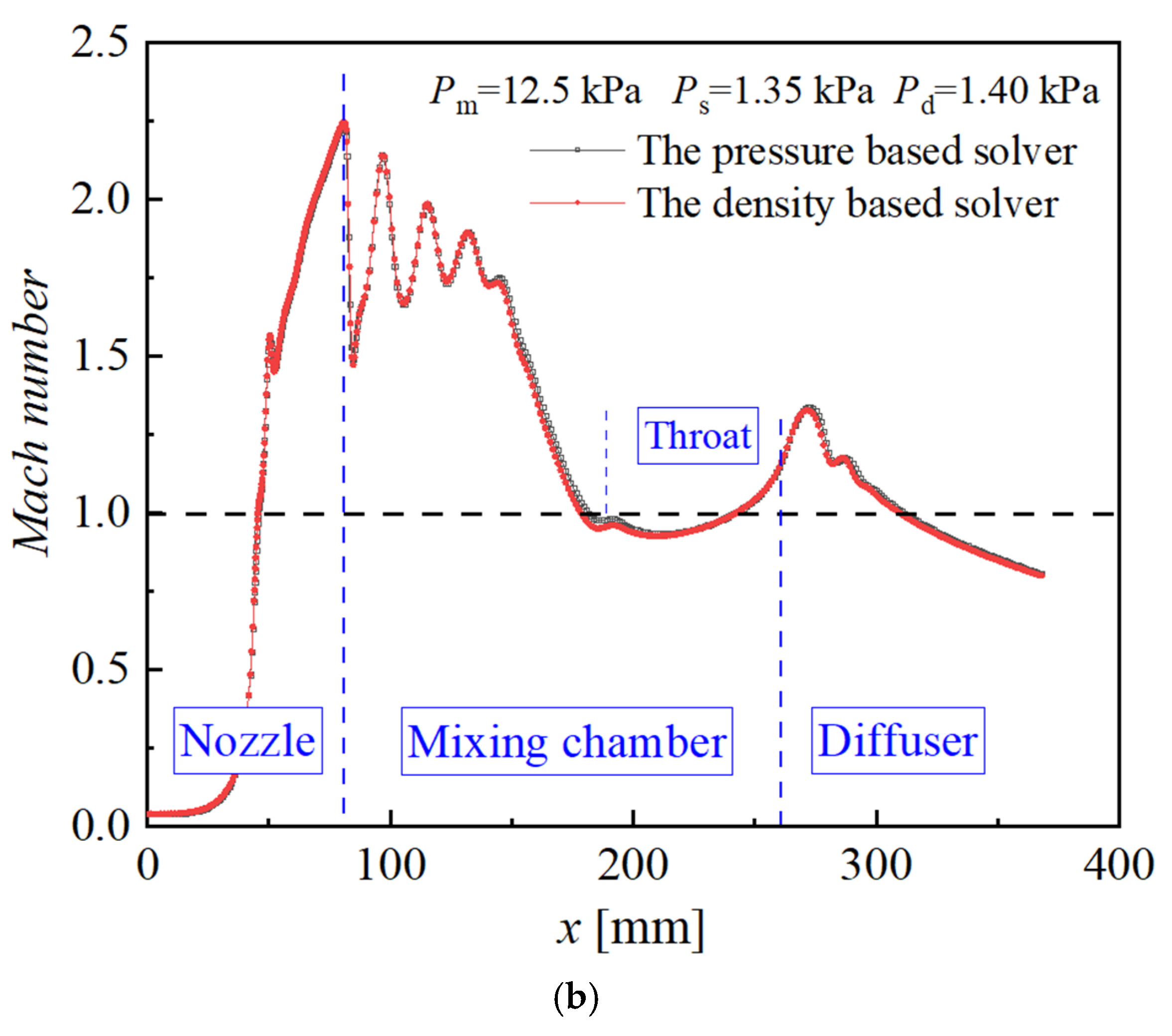
In this chapter, the non-equilibrium condensation model was combined with the k-ω SST turbulence model to perform a comparison of the density-based solver (D-B) and the P-B globally and locally under the same working conditions (Case 8).
Pd* and Ermax obtained by the two solvers are nearly the same. Compared to D-B, Er, Gs, and Gm obtained by P-B are all slightly greater, with maximum differences of 1.2%, 1.7%, and 0.1%, respectively.
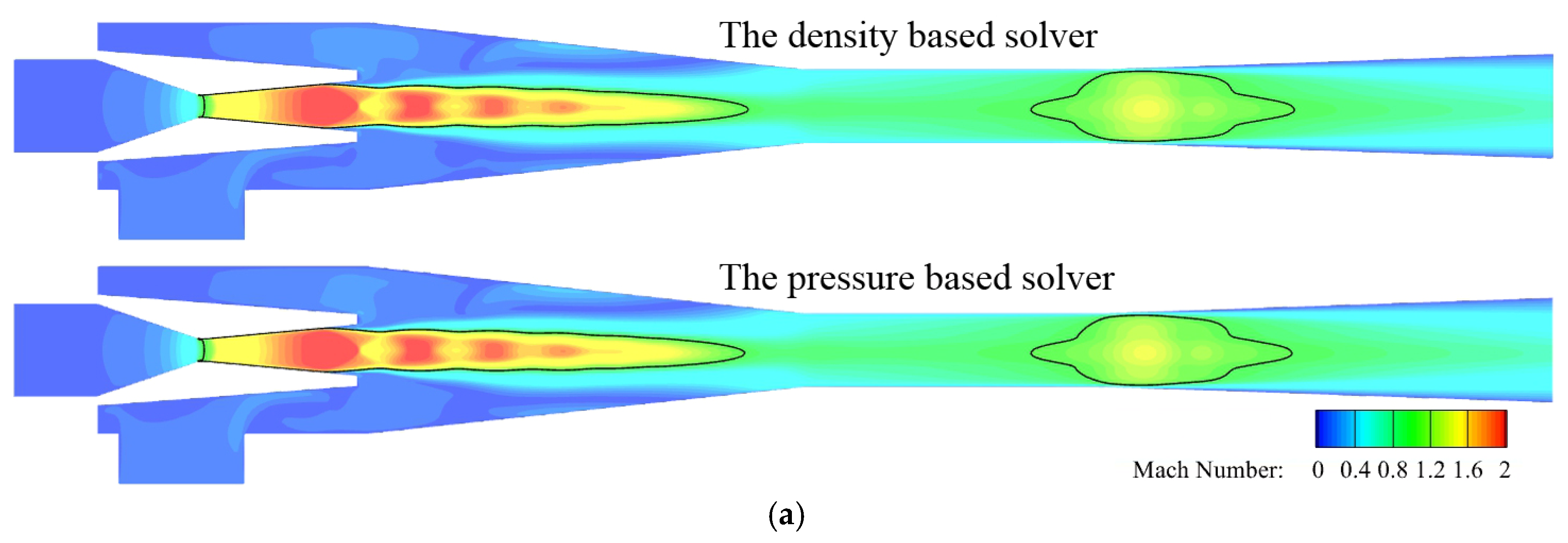
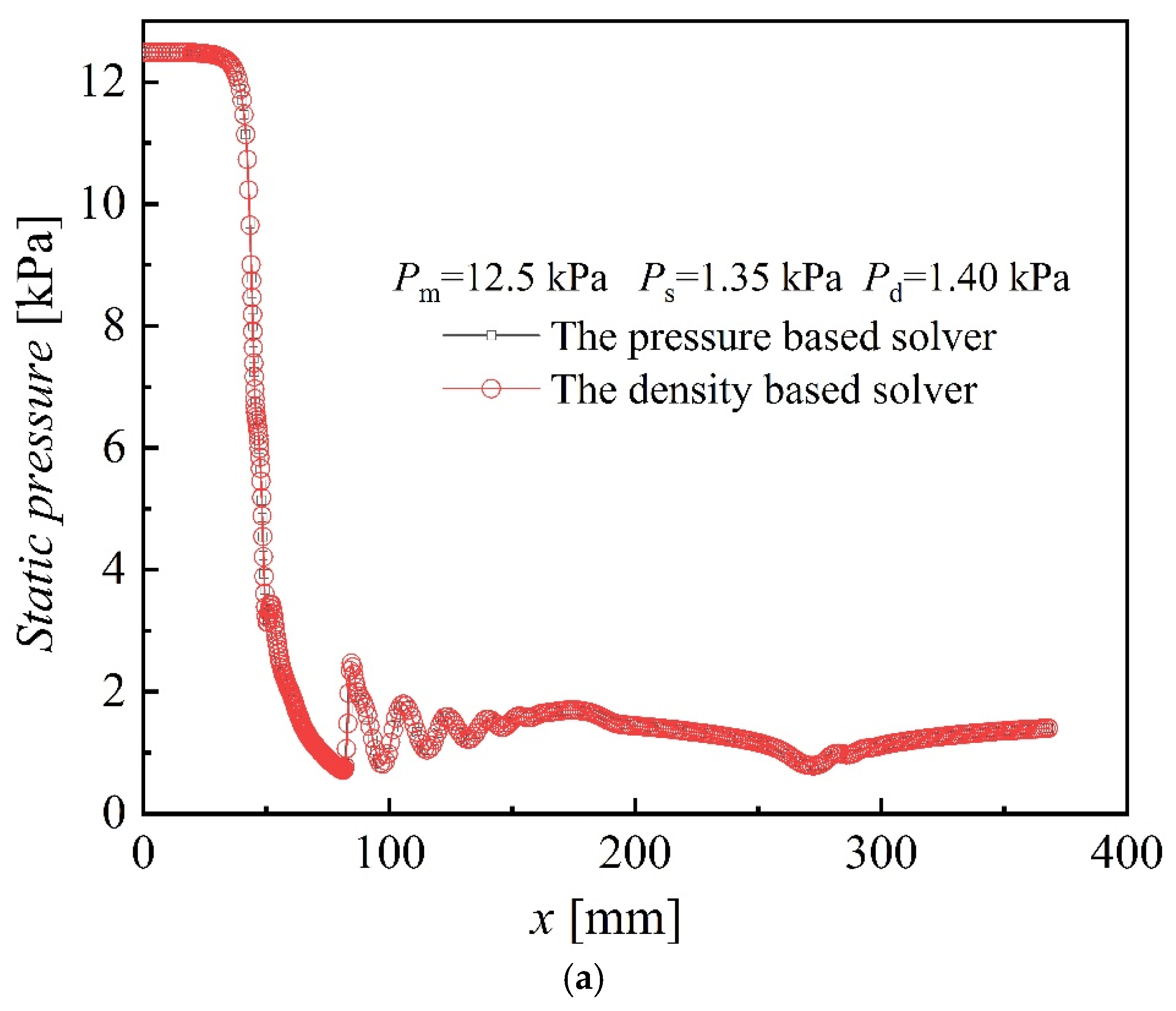
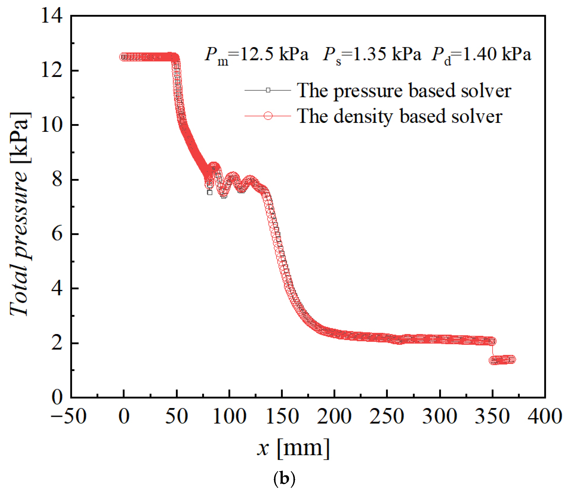
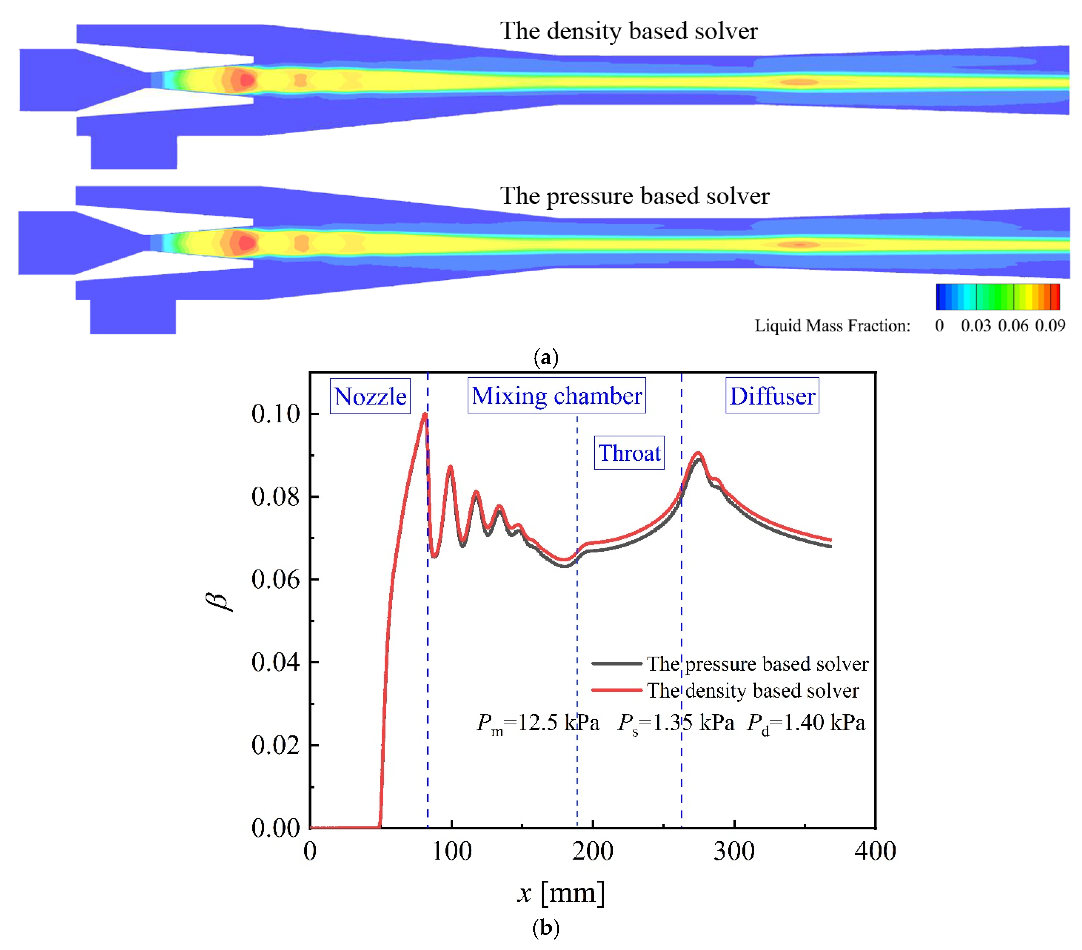
The flow structures that are reflected by contours of Mach number and static pressure simulated by both solvers are almost identical, as shown in Figure 10 and Figure 11. While their liquid mass fraction contours are different around the wall region in the mixing chamber and the diffuser, they are also a little different around the axis, with a maximum relative error of 2.6%, as shown in Figure 12.
According to the convergence criteria reported above, the steps of iterations that reach the convergent condition with the same initialization condition for the two solvers are used for the computational effort and convergence capability analysis. The computational effort of P-B is one-sixth that of D-B. As to the convergence capability, the Courant Number needs to be reduced when D-B is adopted, which greatly increases the computation time and the number of iterations. Moreover, D-B is more sensitive to boundary conditions than P-B. In some other working conditions, D-B cannot achieve convergence while the P-B can. Therefore, the computational effort and convergence capability of P-B are much better than that of D-B, especially after coupling the non-equilibrium condensation model, which results in more computation and harder convergence than those of the ideal-gas model.
In summary, in research and engineering not concerned with condensation phenomena, P-B can be used instead of D-B in simulating high compression with shock wave flow because of its excellent convergence properties and computation saving. However, since D-B can better reflect the physical nature of supersonic fluids, for the sake of rigor, it is still proposed to use D-B in scientific research considering condensation effects and three-dimensional effects.

3.4. Validation, Comparison, and Analysis of 3-D and 2-D Models, Condensation Model, and Ideal-Gas Model

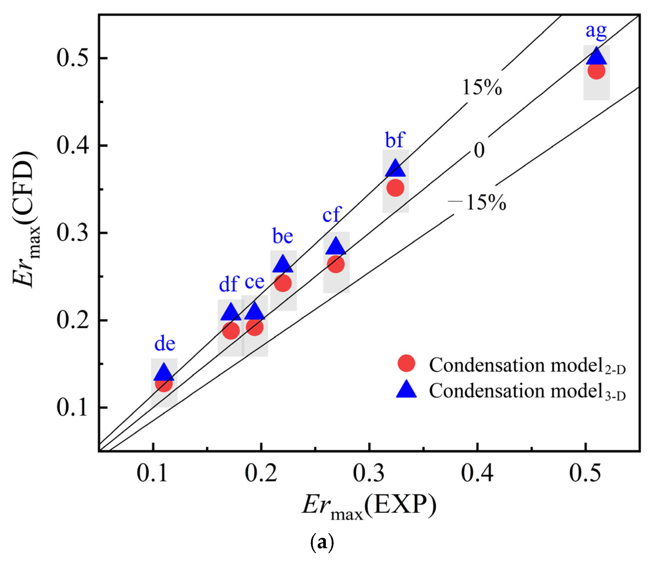
Figure 13a illustrates the validation of ejector performance (Ermax) of the 3-D asymmetric model and 2-D model through validation with Chen and Sun’s experimental data [30]. The average relative error ( e ) of Ermax obtained by the 3-D and 2-D models with the experimental values are −1.9% and 12.8%, respectively, and the maximum relative errors are −8.8% and 25.6%, respectively. This not only verifies the reliability of the CFD model developed in this paper but also shows that, compared with the 2-D axisymmetric model, the 3-D model can reduce the e of the Er between the CFD results and the experimental value by 78.4% and the maximum relative error by 50.0%.
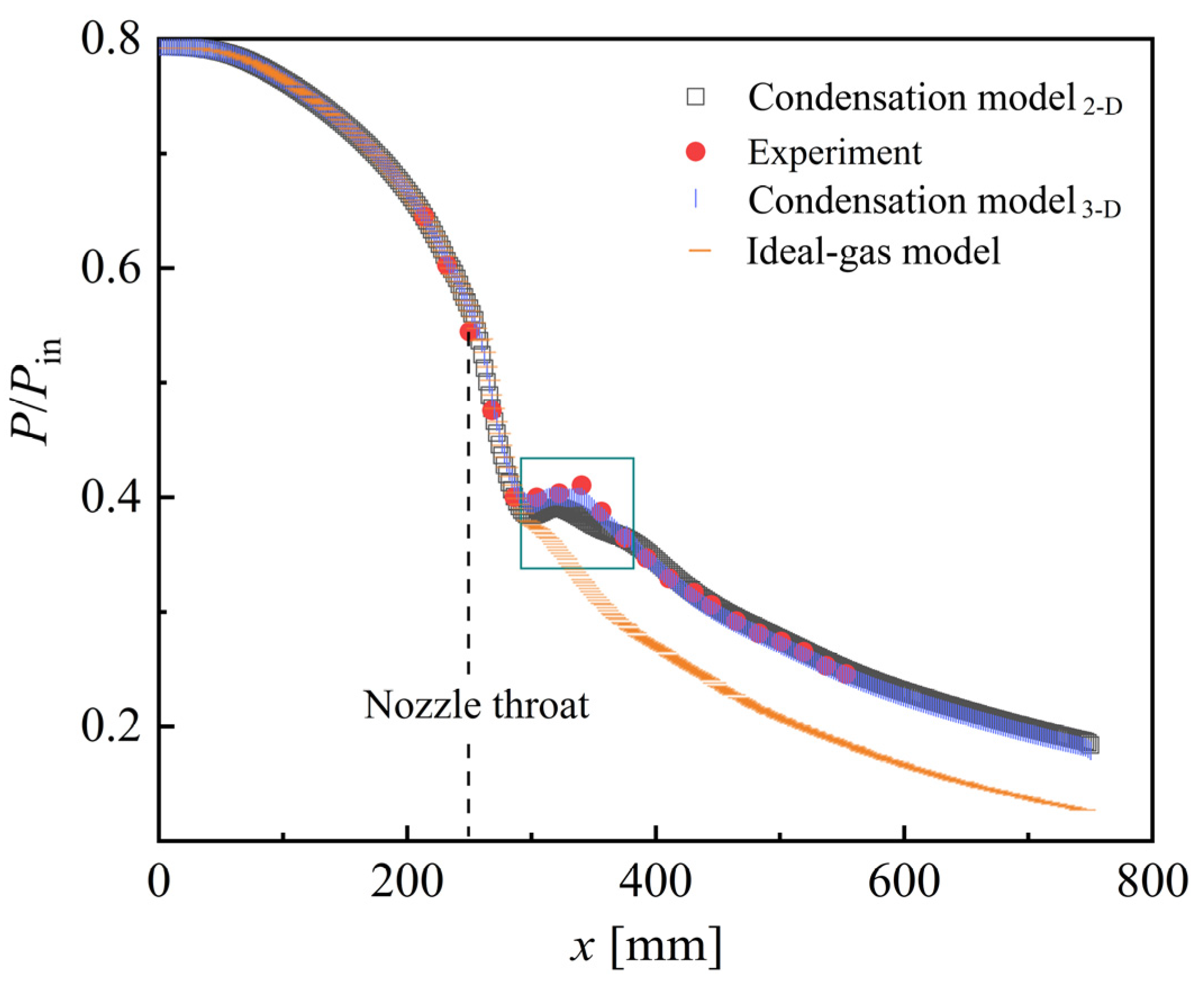
Even though the computational effort and convergence capability of the ideal-gas model are much better than the condensation model, it is proposed to adopt it based on the following two points. As to the ejector performance, compared with the experimental values, the average relative error ( e ) of the Er obtained by the non-equilibrium condensation model is 4.9%, which has a good agreement. In addition, the simulation results of the non-equilibrium condensation model are more consistent with the experimental values than those of the ideal-gas model. Compared with the ideal-gas model, the condensation model can reduce the e of the Er between the CFD results and the experimental value by 72.0% and the maximum relative error by 45.6%, as illustrated in Figure 13b. As to flow phenomena, the condensation model can obtain the condensation shock wave that cannot be obtained by the ideal-gas model, as shown in Figure 14 whose experimental values from the Nozzle A by Moore et al. [38]. When the condensation shock wave appears, the fluid pressure suddenly drops. e of P/Pin obtained by the 3-D model and 2-D model is 1.1% and 1.9%, respectively. The condensation shock wave occurrence position of the 3-D model accords with experiments quite well. In contrast, the position obtained by the 2-D model is 20.02 mm (2.67% of the nozzle length) ahead of the experimental results. The 3-D model results are closer to experiments compared to the 2-D model.
In conclusion, a 3-D asymmetric condensation model with a density-based solver is recommended for simulating steam ejectors accurately.

4. Conclusions

This paper’s originality is that both condensation and 3-D effects on the simulation results have been considered in the comprehensive comparative study of turbulence models, near-wall treatments, and solvers in the RANS equations approach for steam ejectors. Future research can perform a comparative study of the RANS equations and Large Eddy Simulation method based on this paper. The condensation and 3-D effects should be considered. The following conclusions have emerged:
(1)
Considering non-equilibrium condensation and 3-D effects, the k-ω SST model with the low-Re boundary conditions has the most accurate prediction results globally and locally compared with the experiments: (a) The average relative error of Ermax and Pd* are 4% and −15%, (b) the shock wave type and the condensation position are well predicted. Moreover, it has the widest adaptability to working conditions and the best convergence of the seven turbulence models studied in this paper.
(2)
The difference in Ermax predicted by different models depends mainly on their mass flow rates of suction steam (Gs). The minimum difference in Gs predicted by different models is greater than 55%, while the maximum difference in Gm is less than 8%.
(3)
The number and types of shock waves, and the location of condensation phenomenon of different turbulence models, are various. The k-ε series models predict a normal shock in the diffuser while the other models predict a different number of oblique shock waves.
(4)
All other things being equal, the 3-D model can reduce the average relative error of Er by 78.4% compared to the 2-D model and the condensation model can reduce the average relative error of Er by 72.0% compared to the ideal-gas model.
(5)
A 3-D asymmetric condensation model with a density-based solver is recommended for simulating steam ejectors accurately.

Author Contributions

Conceptualization, Y.L. and S.S.; Methodology, Y.L., H.H., D.D., S.S. and D.Z.; Software, S.S.; Validation, D.D. and S.L.; Formal analysis, Y.L., H.H., D.D., D.Z. and S.L.; Investigation, H.H., D.D. and D.Z.; Resources, Y.L. and S.S.; Data curation, H.H.; Writing—original draft, Y.L.; Writing—review & editing, H.H., D.D. and D.Z.; Visualization, D.Z. and S.L.; Supervision, Y.L.; Project administration, Y.L. and S.S.; Funding acquisition, Y.L. All authors have read and agreed to the published version of the manuscript.

Funding

The project was supported by “the Fundamental Research Funds for the Provincial Universities of Liaoning” (No.LJ212410150010).

Data Availability Statement

The raw data supporting the conclusions of this article will be made available by the authors on request.

Conflicts of Interest

Authors Yiqiao Li and Dan Zhou were employed by the company Bingshan Refrigeration & Heat Transfer Technologies Co., Ltd. The remaining authors declare that the research was conducted in the absence of any commercial or financial relationships that could be construed as a potential conflict of interest.

Nomenclature

B[m3/kg]Virial coefficients
C[m6/kg2]Virial coefficients
CP[J/(kg∙K)]Isobaric heat capacity
E[J]Total energy
Er[-]Entrainment ratio
e[%]Relative error
F[N/m3]Source term
G[kg/s]Mass flow rate
h[J/kg]Specific enthalpy
hlv[J/kg]Latent heat of condensation
J[1/s]Nucleation rate
K[W/(m2∙K)]Heat transfer coefficient
k[m2/s2]Turbulent kinetic energy
kB[-]Boltzmann constant
Ma[-]Mach number
P[Pa]Pressure
R[-]Gas-law constant
r[m]Droplet radius
S[-]Super-saturation ratio
s[J/(kg∙mol∙K)]Specific entropy
ST[kg∙K/ (m3∙s)]Viscous dissipative term
T[K] Temperatures
Greek letters
β[-]Liquid mass fraction
Г[kg/s]Liquid mass generation rate
ρ[kg/m3]Density
γ[-]Specific heat capacities ratio
μ[Pa/s]Dynamic viscosity
σ[N/m]Liquid surface tension
η[1/m3]Droplet number density
θ[-]Non-isothermal correction factor
ν[m2/s]Kinematic viscosity
ε[m2/s3]Turbulent dissipation rate
τ[N/m2]Stress tensor
v[m/s]Velocity
Subscripts
sat Saturation
m Motive steam
s Suction steam
d Discharge steam
l Liquid
v Vapor
max Maximum
* Critical
- Average
eff Effective
i,j Space components
Abbreviations
D-B Density-based solver
P-B Pressure-based solver
RSM Reynolds Stress Model
SWF Standard Wall Function
NWF Non-equilibrium Wall Function
EWT Enhanced Wall Treatment
N-S Navier-Stokes
RANS Reynolds-Averaged Navier–Stokes

References

  1. Li, Y.; Shen, S.; Niu, C.; Mu, X.; Zhang, L. The effect of variable motive pressures on the performance and shock waves in a supersonic steam ejector with non-equilibrium condensing. Int. J. Therm. Sci. 2023, 185, 108034. [Google Scholar] [CrossRef]
  2. Li, Y.; Shen, S.; Yang, Y. Three-dimensional characteristics of aerodynamic shockwave and condensation shockwave in steam ejectors. Desalination 2024, 581, 117606. [Google Scholar] [CrossRef]
  3. Wang, X.; Dong, J.; Zhang, G.; Fu, Q.; Li, H.; Han, Y.; Tu, J. The primary pseudo-shock pattern of steam ejector and its influence on pumping efficiency based on CFD approach. Energy 2019, 167, 224–234. [Google Scholar] [CrossRef]
  4. Han, Y.; Wang, X.; Yuen, A.C.Y.; Li, A.; Guo, L.; Yeoh, G.H.; Tu, J. Characterization of choking flow behaviors inside steam ejectors based on the ejector refrigeration system. Int. J. Refrig. 2020, 113, 296–307. [Google Scholar] [CrossRef]
  5. Wen, C.; Karvounis, N.; Walther, J.H.; Ding, H.; Yang, Y. Non-equilibrium condensation of water vapour in supersonic flows with shock waves. Int. J. Heat Mass Transf. 2020, 149, 119109. [Google Scholar] [CrossRef]
  6. Ansys, Inc. Ansys FLUENT 18.0—Theory Guide; Ansys Fluent: Canonsburg, PA, USA, 2019. [Google Scholar]
  7. Besagni, G.; Cristiani, N.; Croci, L.; Guédon, G.R.; Inzoli, F. Computational fluid-dynamics modelling of supersonic ejectors: Screening of modelling approaches, comprehensive validation and assessment of ejector component efficiencies. Appl. Therm. Eng. 2020, 186, 116431. [Google Scholar] [CrossRef]
  8. Besagni, G.; Inzoli, F. Computational fluid-dynamics modeling of supersonic ejectors: Screening of turbulence modeling approaches. Appl. Therm. Eng. 2017, 117, 122–144. [Google Scholar] [CrossRef]
  9. Hemidi, A.; Henry, F.; Leclaire, S.; Seynhaeve, J.M.; Bartosiewicz, Y. CFD analysis of a supersonic air ejector. Part II: Relation between global operation and local flow features. Appl. Therm. Eng. 2009, 29, 2990–2998. [Google Scholar] [CrossRef]
  10. Gagan, J.; Smierciew, K.; Butrymowicz, D.; Karwacki, J. Comparative study of turbulence models in application to gas ejectors. Int. J. Therm. Sci. 2014, 78, 9–15. [Google Scholar] [CrossRef]
  11. Zhu, Y.; Jiang, P. Experimental and numerical investigation of the effect of shock wave characteristics on the ejector performance. Int. J. Refrig. 2014, 40, 31–42. [Google Scholar] [CrossRef]
  12. Croquer, S.; Poncet, S.; Aidoun, Z. Turbulence modeling of a single-phase R134a supersonic ejector. Part 1: Numerical benchmark. Int. J. Refrig. 2016, 61, 140–152. [Google Scholar] [CrossRef]
  13. Ruangtrakoon, N.; Thongtip, T.; Aphornratana, S.; Sriveerakul, T. CFD simulation on the effect of primary nozzle geometries for a steam ejector in refrigeration cycle. Int. J. Therm. Sci. 2013, 63, 133–145. [Google Scholar] [CrossRef]
  14. Han, Y.; Wang, X.; Sun, H.; Zhang, G.; Guo, L.; Tu, J. CFD simulation on the boundary layer separation in the steam ejector and its influence on the pumping performance. Energy 2019, 167, 469–483. [Google Scholar] [CrossRef]
  15. Varga, S.; Soares, J.; Lima, R.; Oliveira, A.C. On the selection of a turbulence model for the simulation of steam ejectors using CFD. Int. J. Low-Carbon Technol. 2017, 12, 233–243. [Google Scholar] [CrossRef]
  16. Wu, J.; Xu, P.; Li, L.; Li, Z.; Qi, H.; Wang, C.; Zhang, Y.; Xie, Y.; Tan, D. Multiphase dynamic interfaces and abrasive transport dynamics for abrasive flow machining in shear thickening transition states. Powder Technol. 2024, 446, 120150. [Google Scholar] [CrossRef]
  17. Tan, Y.; Ni, Y.; Xu, W.; Xie, Y.; Li, L.; Tan, D. Key technologies and development trends of the soft abrasive flow finishing method. J. Zhejiang Univ.-Sci. A 2023, 24, 1043–1064. [Google Scholar] [CrossRef]
  18. Aidoun, Z.; Ameur, K.; Falsafioon, M.; Badache, M. Current Advances in Ejector Modeling, Experimentation and Applications for Refrigeration and Heat Pumps. Part 1: Single-Phase Ejectors. Inventions 2019, 4, 15. [Google Scholar] [CrossRef]
  19. Li, C.; Li, Y.Z. Investigation of entrainment behavior and characteristics of gas-liquid ejectors based on CFD simulation. Chem. Eng. Sci. 2011, 66, 405–416. [Google Scholar] [CrossRef]
  20. Yazdani, M.; Alahyari, A.A.; Radcliff, T.D. Numerical modeling of two-phase supersonic ejectors for work-recovery applications. Int. J. Heat Mass Transf. 2012, 55, 5744–5753. [Google Scholar] [CrossRef]
  21. Sriveerakul, T.; Aphornratana, S.; Chunnanond, K. Performance prediction of steam ejector using computational fluid dynamics: Part 1. Validation of the CFD results. Int. J. Therm. Sci. 2007, 46, 812–822. [Google Scholar] [CrossRef]
  22. Tashtoush, B.M.; Moh’d A, A.N.; Khasawneh, M.A. A comprehensive review of ejector design, performance, and applications. Appl. Energy 2019, 240, 138–172. [Google Scholar] [CrossRef]
  23. Cai, L.; He, M.; Huang, K.Z.; Xiong, W. Computational fluid dynamics simulation of the supersonic steam ejector using different condensation model. Therm. Sci. 2019, 23, 236. [Google Scholar] [CrossRef]
  24. Mazzelli, F.; Little, A.B.; Garimella, S.; Bartosiewicz, Y. Computational and experimental analysis of supersonic air ejector: Turbulence modeling and assessment of 3D effects. Int. J. Heat Fluid Flow 2015, 56, 305–316. [Google Scholar] [CrossRef]
  25. Young, J.B. An equation of state for steam for turbomachinery and other flow calculations. J. Eng. Gas Turbines Power 1988, 110, 1–7. [Google Scholar] [CrossRef]
  26. Young, J.B. Spontaneous condensation of steam in supersonic nozzles. PCH Physicochem. Hydrodyn. 1982, 3, 57–82. [Google Scholar]
  27. Kong, N.; Qi, Z. Influence of speed of sound in two-phase region on 1-D ejector performance modelling. Appl. Therm. Eng. 2018, 139, 352–355. [Google Scholar] [CrossRef]
  28. Daiguji, H.; Ishazaki, K.; Ikohagi, T. A high-resolution numerical method for transonic non-equilibrium condensation flows through a steam turbine cascade. Proc. 6th Int. Symp. Comput. Fluid Dyn. 1995, 1, 479–484. [Google Scholar]
  29. Senoo, S.; Shikano, Y. Two-dimensional analysis for non-equilibrium homogeneously condensing flows through steam turbine cascade. JSME Int. J. Ser. B Fluids Therm. Eng. 2002, 45, 865–871. [Google Scholar] [CrossRef]
  30. Chen, Y.; Sun, C. Experimental study of the performance characteristics of a steam-ejector refrigeration system. Exp. Therm. Fluid Sci. 1997, 15, 384–394. [Google Scholar] [CrossRef]
  31. Zhang, G.; Zhang, X.; Wang, D.; Jin, Z.; Qin, X. Performance evaluation and operation optimization of the steam ejector based on modified model. Appl. Therm. Eng. 2019, 163, 114388. [Google Scholar] [CrossRef]
  32. Zhang, G.; Dykas, S.; Li, P.; Li, H.; Wang, J. Accurate condensing steam flow modeling in the ejector of the solar-driven refrigeration system. Energy 2020, 212, 118690. [Google Scholar] [CrossRef]
  33. Wang, X.; Dong, J.; Li, A.; Lei, H.; Tu, J. Numerical study of primary steam superheating effects on steam ejector flow and its pumping performance. Energy 2014, 78, 205–211. [Google Scholar] [CrossRef]
  34. Ariafar, K.; Buttsworth, D.; Al-Doori, G.; Malpress, R. Effect of mixing on the performance of wet steam ejectors. Energy 2015, 93, 2030–2041. [Google Scholar] [CrossRef]
  35. Mazzelli, F.; Giacomelli, F.; Milazzo, A. CFD modeling of condensing steam ejectors: Comparison with an experimental test-case. Int. J. Therm. Sci. 2018, 127, 7–18. [Google Scholar] [CrossRef]
  36. Zhang, G.; Wang, X.; Pourranjbar, D.; Dykas, S.; Li, H.; Chen, J. The comprehensive analysis of the relationship between the latent heat, entrainment ratio, and ejector performance under different superheating degree conditions considering the non-equilibrium condensation. Appl. Therm. Eng. 2022, 200, 117701. [Google Scholar] [CrossRef]
  37. Li, Y.; Niu, C.; Shen, S.; Mu, X.; Zhang, L. Double choking characteristics of three-dimensional steam ejector with non-equilibrium condensing. Appl. Therm. Eng. 2022, 211, 118446. [Google Scholar] [CrossRef]
  38. Moore, M.J.; Walters, P.T.; Crane, R.I.; Davidson, B.J. Predicting the fog-drop size in wet-steam turbines. In Proceedings of the IMechE Conference on Heat and Fluid Flow in Steam and Gas Turbine Plant, Coventry, UK, 3–5 April 1973; pp. C37–C73. [Google Scholar]
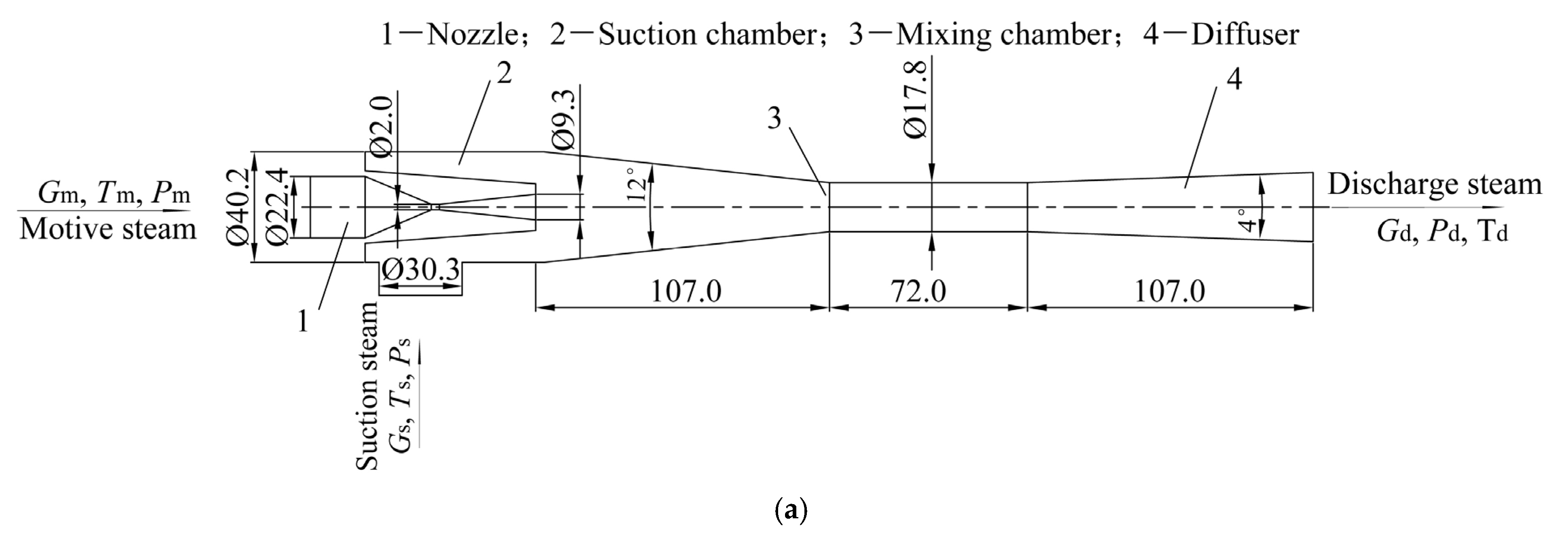
Figure 1. Two sizes of steam ejectors. (a) Size of E1. (b) Size of E2.
Energies 17 05586 g001aEnergies 17 05586 g001b
Figure 2. Information of steam ejector meshes. (a) Steam ejector meshes. (b) y+ profile along ejector wall.
Energies 17 05586 g002
Figure 3. First type mesh independence study of different models. (a) Grid independence study with Case 1. (b) Grid independence study with Case 4.
Energies 17 05586 g003
Figure 4. Second type mesh independence study of different models. (a) Grid independence study with Case 1. (b) Grid independence study with Case 4.
Energies 17 05586 g004aEnergies 17 05586 g004b
Figure 5. Histogram of the prediction error.
Energies 17 05586 g005
Figure 6. Relative errors of Pd*.
Energies 17 05586 g006
Figure 7. Mach number profiles of the axis under Case 4 with Pd = 1335 Pa.
Energies 17 05586 g007
Figure 8. Mach number contours under Case 4 with Pd = 1335 Pa.
Energies 17 05586 g008
Figure 9. β contours under Case 4 with Pd = 1335 Pa.
Energies 17 05586 g009
Figure 10. Mach number distributions with different solvers. (a) Mach number contours with different solvers. (b) Mach number profiles of the axis.
Energies 17 05586 g010aEnergies 17 05586 g010b
Figure 11. Pressure profiles of the axis with different solvers. (a) Static pressure profiles of the axis with different solvers. (b) Total pressure profiles of the axis with different solvers.
Energies 17 05586 g011aEnergies 17 05586 g011b
Figure 12. Liquid mass fraction distributions with different solvers. (a) Liquid mass fraction contours with different solvers. (b) Liquid mass fraction profiles of the axis.
Energies 17 05586 g012
Figure 13. Ermax of different models and experiments comparison. (a) Comparison of the 2-D and 3-D models. (b) Comparison of the condensation model and the ideal-gas model.
Energies 17 05586 g013aEnergies 17 05586 g013b
Figure 14. P/Pin of different models and experiments comparison.
Energies 17 05586 g014
Table 1. Computation parameters.
SizeCasePm [kPa]Tm [°C]Ps [kPa]Ts [°C]Pd [kPa]
E11116.0105.81.30610.81.35~2.70
2153.0114.21.30610.81.35~2.90
3198.0121.81.30610.81.35~3.90
E2411.90651.31.30610.81.35~1.90
515.46556.61.30610.81.35~2.40
619.57161.61.30610.81.35~2.90
719.57161.61.81315.81.85~2.90
812.552.21.3511.41.4
ag11.90651.31.81315.81.85~2.00
bf15.46556.21.30610.81.35~2.40
cf19.57161.61.30610.81.35~2.90
df24.83766.81.30610.81.35~3.20
be15.46556.21.013.21.1~2.2
ce19.57161.61.013.21.1~2.6
de24.83766.81.013.21.1~3.3
Table 2. Number of cells.
Type1, y+ ≈ 1Type2, Minimum y+ = 30
Mesh LevelCoarseMediumFineCoarseMediumFine
Number [million]0.8 2.0 2.9 0.2 0.4 0.9
Table 3. Relative errors of maximum Er.
Modele(Ermax)
Casek-ω Standard
(EWT)
k-ω
SST
(EWT)
Transition
SST
(EWT)
k-ε Standard
(SWF)
k
RNG
(SWF)
k-ε
Realizable
(SWF)
Linear RSM (SWF)
143%7%−26%−24%−20%−21%5%
247%11%−38%−38%−36%−28%11%
328%2%−31%−40%−37%−30%−19%
442%9%−13%−10%−5%−6%−2%
521%6%−49%−62%−52%−38%−19%
622%−5%−27%−76%−74%−55%−10%
738%−2%−30%−27%−32%−22%−2%
e (Ermax)34.5%4.0%−30.6%−39.5%−36.5%−28.6%−5.2%
Table 4. The average difference of the mass flow rate predicted by seven turbulence models.
Δ G Δ G m Δ G s
Case
18%67%
22%93%
35%88%
44%55%
57%96%
62%129%
77%80%
average5%87%
Table 5. Relative computational effort required for solving Case 8 with different turbulence models.
k-ω Standard (EWT)k-ω SST (EWT)Transition SST (EWT)k-ε Standard
(EWT)
k-ε RNG
(EWT)
k-ε Realizable
(EWT)
RSM
(EWT)
1.31.63.611.51.44.2
Disclaimer/Publisher’s Note: The statements, opinions and data contained in all publications are solely those of the individual author(s) and contributor(s) and not of MDPI and/or the editor(s). MDPI and/or the editor(s) disclaim responsibility for any injury to people or property resulting from any ideas, methods, instructions or products referred to in the content.