Article

Research on the Mechanism and Prediction Model of Pressure Drive Recovery in Low-Permeability Oil Reservoirs

by
Haicheng Liu
1,2,* and
Binshan Ju
1,*
1
School of Energy Resources, China University of Geosciences (Beijing), Beijing 100083, China
2
Exploration and Development Research Institute of Sinopec Shengli Oilfield Company, Dongying 257015, China
*
Authors to whom correspondence should be addressed.
Energies 2024, 17(21), 5253; https://doi.org/10.3390/en17215253
Submission received: 29 August 2024 / Revised: 15 October 2024 / Accepted: 16 October 2024 / Published: 22 October 2024

Abstract

:
China boasts significant reserves of low-permeability oil reservoirs, and the economic and efficient development of these reservoirs plays a crucial role in enhancing oil and gas production. However, the “difficult injection and difficult recovery” issue in low-permeability oil reservoirs is a major challenge. To address this, research is conducted on the mechanism of pressure drive based on the mathematical model of oil-water seepage in low-permeability reservoirs and the model of fracture permeability. The study finds that pressure drive technology, by directly delivering the pressure drive agent deep into the low-permeability reservoir, effectively prevents viscosity loss and adhesion retention of the agent in the near-wellbore area. This technology expands the swept volume, improves oil washing efficiency, replenishes formation energy, and facilitates the gathering and production of scattered remaining oil. For reservoirs with higher permeability, pressure drive yields quick results, and high-pressure water injection can be directly adopted for pressure drive to reduce costs. On the other hand, reservoirs with lower permeability have difficulty in water absorption, and the use of surfactant-based pressure drive can effectively reduce the seepage resistance of the reservoir, enhancing its water absorption capacity and improving development outcomes. Based on the mechanism of pressure drive development, further research is conducted on the production characteristics of pressure drive mines. Addressing the variability in pressure drive effects, big data analysis tools such as SHAP analysis and correlation analysis are employed to evaluate the main controlling factors of pressure drive in both new and old areas. Additionally, non-time series and time series pressure drive production forecasting models are established based on pressure drive data.

1. Introduction

Currently, 70% of global oil production originates from mature oilfields, and they will continue to serve as the primary source of oil output in the future [1,2]. Mature oilfields, having undergone prolonged water injection and multiple chemical enhanced oil recovery (EOR) stages, are characterized by high recovery rates and water cuts, posing significant challenges for further development and exploitation in China’s petroleum industry. For instance, the Daqing oilfield’s low-to-medium permeability reservoirs exhibit comprehensive water cuts ranging from 93% to 96% and recovery rates of 38% to 42%, with substantial remaining reserves [3,4,5,6]. However, these reserves are hindered by poor reservoir quality, scattered remaining oil distributions, and injection–production difficulties, rendering further enhancement of recovery rates challenging. Thus, there is an urgent need for efficient reservoir stimulation technologies that can improve reservoir utilization and mobilize scattered remaining oil [7,8,9,10,11,12].
Xue Changrong [13] analyzed oil recovery and fracturing techniques for low-permeability reservoirs based on practical work experience, offering insights yet lacking empirical validation and in-depth studies on production efficiency. Ren Zeying [14] demonstrated the application of an integrated geological-engineering approach in the low-permeability turbidite sandstone reservoir in the Niuzhuang Sag of the Dongying Depression, significantly enhancing reservoir characterization, drilling efficiency, and oil displacement. While this technology shows promise, it also complicates operations and may slow production rates. Lan Shuang [15] theoretically explored the potential of micro-nano emulsions as enhanced water injection agents for low-permeability reservoirs, highlighting the need for practical implementation and further investigation. The morphological complexity and orientation disorder of pore space evolution during in-situ thermal reconstruction of oil shale, and their effects on permeability are introduced. Pan Duo [16] introduced various EOR technologies, including polymer flooding, composite flooding, microbial flooding, and in-depth profile control, to improve recovery in low-permeability reservoirs. However, these techniques are complex and technically demanding. Liu Jun [17] paid attention to this issue of morphological complexity and azimuthal disorder of evolving pore space in low-maturity oil shale during in-situ thermal upgrading, and impacts on permeability.
Yu Jinzhu [18] reviewed fracturing techniques and trends for low-permeability oilfields, focusing on the state-of-the-art without addressing specific efficiency issues or proposing innovative solutions. Yang Yong [19] conducted numerical simulations to study the impact of various pressure-driven parameters on production enhancement in low-permeability reservoirs. While it identified optimal parameter combinations, the study did not fully address injection difficulties. The evolution of the anisotropic thermophysical properties of low-maturity oil shales under elevated temperatures has been investigated, and a rational prediction of its impact on the restoration of oil development has been conducted [20]. Zhang, S.Q [21] employed a petrophysical and geochemical investigation-based methodology to conduct a multilithology analysis of the reservoir in the Permian Longtan Formation of the southeastern Sichuan Basin, and provided a framework for pressure-driven exploitation. Li, L. [22] studied the distribution and development methods of coal measure gas resources in China, and pressure-driven exploitation was proposed as an important development approach. Cui Chuanzhi [23] analyzed the effects of induced fractures on injection well pressures during pressure-driven water injection, contributing to the understanding of unstable seepage mechanisms but lacking a comprehensive assessment of the impact on oil recovery.
Conventional chemical flooding in low-to-medium permeability reservoirs suffers from low injection efficiency, poor reservoir utilization, and high chemical loss. Traditional hydraulic fracturing establishes high-flow channels but struggles with energy replenishment and sweep efficiency. Researchers have proposed large-scale pressure-driven fracturing, which outperforms conventional chemical flooding and hydraulic fracturing in field tests [24,25,26,27]. However, the coupling mechanisms between hydraulic fractures and chemical flooding, as well as the oil displacement mechanisms during chemical agent elastic flowback, remain unclear [28,29,30]. Furthermore, a systematic approach to studying fluid flow patterns and enhanced recovery outcomes during pressure-driven processes is lacking, hindering large-scale application [31,32,33,34].
Previous scholars have conducted extensive research on enhancing the recovery efficiency of low-permeability and tight reservoirs, covering a wide range of aspects. Among these [35,36], they investigate the computational methods for determining well spacing in CO2 miscible and immiscible flooding, aiming to optimize the efficiency of CO2 flooding. They employ 3D numerical simulations to study the dynamic propagation of fractures in hydraulic fracturing of low-permeability reservoirs, providing a theoretical basis for fracturing design [37]. The optimal well spacing deployment patterns for low-permeability lens-shaped lithological reservoirs to optimize well pattern design are employed [38]. They introduce the application of an advanced water injection model in low-permeability reservoirs to enhance the effectiveness of waterflooding [39]. The application of volume fracturing technology in tight oil reservoirs is examined and its potential for improving recovery rates is demonstrated [40]. Overall, these studies provide scientific evidence and technical support for the effective development of low-permeability and tight reservoirs; however, there are still several issues that have not been considered.
The effect of pressure drive oil recovery we have studied is more detailed. A is rich in low-permeability reservoir resources, with a total of 428 well groups implemented in low-permeability reservoirs, resulting in an accumulated oil increase of 371,000 tons. This study will demonstrate that pressure drive in low-permeability reservoirs can effectively solve the problem of “difficult injection and difficult recovery”. By establishing a mathematical model for oil-water seepage in low-permeability reservoirs and a model of fracture permeability, we investigate the development mechanism of pressure drive. This addresses the challenges of difficult economic production in low-abundance beach-bar sand reservoirs, the issue of interlayer utilization differences in low-permeability reservoirs, and the general problems of poor sweep efficiency and low recovery rates in low-permeability reservoirs. In view of the differences in the effects of pressure drive, big data analysis methods such as SHAP analysis and correlation analysis are used to evaluate the main controlling factors of pressure drive in new and old areas. A non-time series and time series pressure-driven production capacity prediction model based on pressure-driven data-driven has been established. The non-time series pressure-driven production capacity prediction model based on machine learning has high accuracy and has been verified.

2. Materials and Methods

2.1. Mathematical Model of Oil-Water Seepage in Low-Permeability Reservoirs

The pressure analysis model for pressure-driven water injection wells comprises two primary components: the mathematical model of oil-water seepage under pressure-driven water injection and the fracture propagation model during such injection. Prior to establishing the pressure analysis model, the following assumptions are made: ① Two-dimensional planar flow; ② The reservoir only involves oil-water two-phase seepage, with oil and water being immiscible and individually adhering to Darcy’s law; ③ Both rock and fluids are slightly compressible; ④ Heterogeneity and anisotropy of the rock are considered; ⑤ The effect of gravity is neglected; ⑥ The fracture propagation is modeled as a composite linear expansion. Utilizing a quarter of the five-spot well pattern as the research unit, a pressure analysis model for pressure-driven water injection is formulated.
Oil Phase Seepage Equation:
    x p o k x k r o μ o p o x G o + y p o k y k r o μ o p o y G o + q o = t φ p o s o
Water Phase Seepage Equation:
    x p w k x k r w μ w p w x G w + y p w k y k r w μ w p w y G w + q w = t φ p w s w
Auxiliary Equation:
  S o + S w = 1
In the equations, x and y represent the lengths along the x-direction and y-direction, respectively, in meters (m); t is time, in seconds (s); Kx and Ky are the absolute permeabilities in the x-direction and y-direction, respectively, of the porous medium in the reservoir, in Darcy (D); Kro and Krw are the relative permeabilities of the oil phase and water phase, respectively; ρo and ρw are the densities of the oil phase and water phase, respectively, in kilograms per cubic meter (kg/m3); µo and µw are the viscosities of the oil phase and water phase, respectively, in milli Pascal-seconds (m Pa·s); φ represents the porosity of the porous medium in the reservoir; qo and qw are the oil phase and water phase production rates under standard conditions, respectively, in cubic meters per day (m3/d); po and pw are the pressures of the oil phase and water phase, respectively, in megapascals (MPa); G is the threshold pressure gradient, in megapascals per meter (MPa/m); So and Sw are the saturation of the oil phase and water phase, respectively.
By combining the initial conditions, internal and external boundary conditions with Equations (1)–(3), a two-phase oil-water seepage model can be constructed.

2.2. Model of Fracture Permeability

The exponential model is currently the most widely used mathematical model for stress sensitivity, which describes the relationship between formation pressure and fracture permeability.
  K = K 0 e α σ
  σ = σ o p
In the equation, K represents the fracture permeability, in Darcy (D); K0 is the initial fracture permeability, also in Darcy (D); α is the dimensionless stress sensitivity coefficient; σ is the effective stress, in megapascals (MPa); σ0 is the overburden pressure, in megapascals (MPa); and p is the formation pore pressure, also in megapascals (MPa).
Based on previous studies on the relationship between formation pressure and fracture permeability, a fracture permeability model under pressure-driven conditions is established:
When the formation pressure is in the ascending stage:
K = K i , p p c K = K c e α 1 ( σ 0 p ) p > p c
When the formation pressure is in the descending stage:
K = K min e α 2 σ 0 p , p = p min K = K min p < p min
In the formula, α1 and α2 represent the dimensionless stress sensitivity coefficients obtained through fitting.

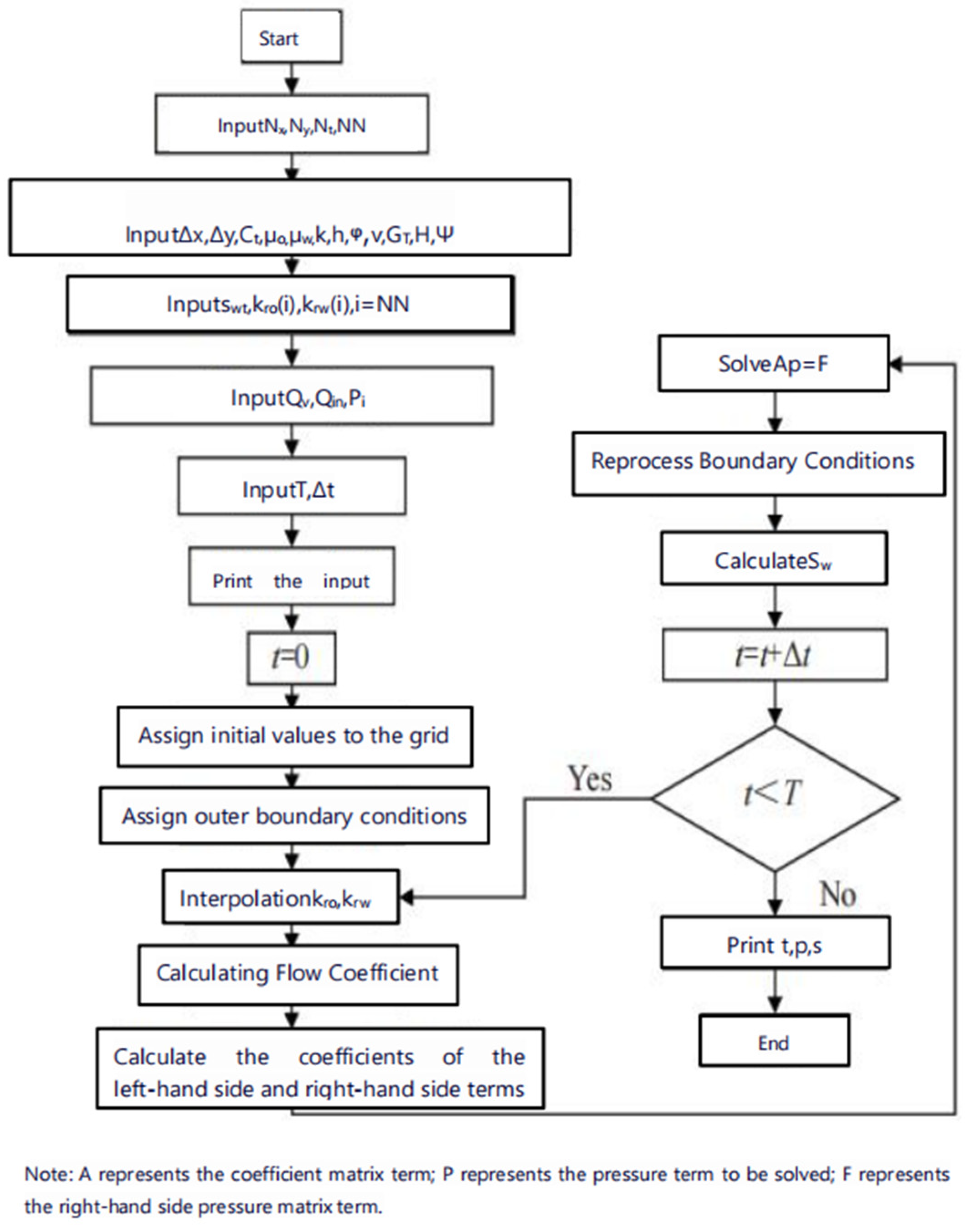
2.3. Solution of Pressure-Driven Model

The pressure analysis model for pressure-driven water injection wells describes a fluid–solid coupling and oil-water two-phase nonlinear seepage problem, which is challenging to solve analytically or semi-analytically. Therefore, the model is discretized, and the finite difference method is employed to find its solution. In the differential equations governing the seepage of oil and water phases, the right-hand side terms are discretized using the first-order forward difference, while the left-hand side terms are discretized using the second-order central difference. The unknowns are po, pw, so, sw, with the independent variables being (x, y, t). Expanding the differential equations for oil and water phases through discretization, the difference equations for the oil and water phases are obtained as follows:
T o y j 1 2 p o i , j 1 n + 1 + T o x j 1 2 p o i 1 , j n + 1 T o x i + 1 2 + T o x i 1 2 + T o y j + 1 2 + T o y j 1 2 + V i , j β o i , j Δ t p o i 1 , j n + 1 + T o x j + 1 2 p o i + 1 , j n + 1 + T o x j + 1 2 p o i , j + 1 n + 1 = V p i , j ρ o i , j s o i , j n + 1 s o i , j n Δ t Q o i , j V i , j β o i , j Δ t p o i , j n
T w y j 1 2 p w i , j 1 n + 1 + T w x j 1 2 p w i 1 , j n + 1 T w x j + 1 2 + T w x j 1 2 + T w x j + 1 2 + T w x j 1 2 + V i , j β w i , j Δ t p w i . j n + 1 + T w x j + 1 2 p w i + 1 , j n + 1 + T w x j + 1 2 p w i + 1 , j n + 1 = V p i , j β w i , j s w i , j n + 1 s w i , j n Δ t Q w i , j V i , j β w i , j Δ t p w i . j n
In this context,
T o y j ± 1 2 = λ o y j ± 1 2 Δ x i h 0.5 Δ y j + Δ y j ± 1 T o x j ± 1 2 = λ o x j ± 1 2 Δ y j h 0.5 Δ x i + Δ x i ± 1 , T w y j ± 1 2 = λ w y j ± 1 2 Δ x i h 0.5 Δ y j + Δ y j ± 1 T w y j ± 1 2 = λ w x j ± 1 2 Δ y i h 0.5 Δ x j + Δ x j ± 1 , λ o = ρ o k k r o μ o , λ w = ρ w k k r w μ w β 0 = ρ o φ s o C p + C o , β w = ρ w φ s w C p + C w V i , j = Δ x i Δ y j h , Q o i , j = q o i , j Δ x i Δ y i h , Q w i , j = q w i , j Δ x i Δ y j h V p i , j = φ i , j Δ x i Δ y j h
In Equations (8) to (9), Δxi represents the unit grid length in the x-direction, with units of meters (m). Δyj represents the unit grid length in the y-direction, with units of meters (m). Δt represents the unit time, with units of days (d). p o i , j n + 1 is the oil phase pressure at node (i,j) and time step (n + 1), with units of MPa. s o i , j n + 1 is the oil saturation at node (i,j) and time step (n + 1). p w i , j n + 1 is the water phase pressure at node (i,j) and time step (n + 1), with units of MPa. s w i , j n + 1 is the water saturation at node (i,j) and time step (n + 1). Cp is the rock compressibility coefficient. Co is the oil phase compressibility coefficient. Cw is the water phase compressibility coefficient. Vi,j is the volume of grid (i,j), with units of cubic meters (m3). Qoi,j,Qwi,j are the production or injection rates of grid (i,j), with units of cubic meters per day (m3/d). Vpi,j is the pore volume of grid (i,j), with units of cubic meters (m3). T o x i ± 1 2 , T o x i ± 1 2 , T o y j ± 1 2 , T o y j ± 1 2 are the relative permeabilities of the water and oil phases, respectively. Using the IMPES (Implicit Pressure, Explicit Saturation) method to implicitly solve for pressure s o = 1 s w , we can let A = ρ o ρ w represent porosity and [ K W f = W x , t 3 12 × 10 9 ( 8 ) ] × A , represent the absolute permeability. By introducing these notations and eliminating the saturation terms from the above equations, we focus on solving for pressure implicitly. Additionally, KWf represents the fracture conductivity, with units of 10−3 μm2·m.
c i , j p o i , j 1 n + 1 + a i , j p o i 1 , j n + 1 + e i , j p o i , j n + 1 + b i , j p o i + 1 , j n + 1 + d i , j p o i , j + 1 n + 1 = f i , j
Wherein:
c i , j = T o y j 1 2 + A T w y j 1 2 a i , j = T o x i 1 2 + A T w x i 1 2 e i , j = T o x i 1 2 + T o x i + 1 2 + T o y j 1 2 + T o y j + 1 2 + V i , j β o i , j Δ t A T W x i 1 2 + T W x i + 1 2 + T W y j 1 2 + T W y j + 1 2 + V i , j β W i , j Δ t b i . j = T o x i + 1 2 + A T w x i + 1 2 d i . j = T o y j + 1 2 + A T o y j + 1 2 f i , j = Q o i , j + V i , j β o i , j Δ t p o i , j n A Q w i , j + V i , j β w i , j Δ t p w i , j n
At each node, by applying Equation (11) to formulate equations, a pentadiagonal system of equations is obtained. By substituting the initial and boundary conditions into this system of equations, the pressure can be solved. Subsequently, the pressure values obtained are substituted into the water phase difference Equation (9) to explicitly solve for the water saturation. Finally, the fracture length, conductivity, pressure, and saturation distributions are updated, and the simulation calculation for the next time step is carried out, thereby achieving the solution of the pressure analysis model for pressure-driven water injection wells.
In the solution flowchart of the pressure-driven water injection well pressure analysis model depicted in Figure 1, the notations Nx, Ny, Nt, and NN represent the number of grid nodes in the x-direction, the number of grid nodes in the y-direction, the number of time steps, and the total number of iterations, respectively. T denotes the total simulation time.
During the process of solving the pressure-driven water injection well pressure analysis model, the following steps are typically followed:
(1)
Input Basic Parameters: Initially, the fundamental parameters required by the model are input. These parameters may include rock and fluid properties, well specifications, and operational conditions.
(2)
Initialization and Boundary Conditions: Each grid cell is assigned an initial value, and the outer boundary conditions of the model are specified. These boundary conditions define the pressure or flow conditions at the edges of the simulated reservoir.
(3)
Calculation of kro and krw: Using interpolation methods, the relative perm of oil (kro) and water (krw) are determined for each grid cell. These values are crucial in determining the flow behavior of the fluids within the reservoir.
(4)
Calculation of Flow Coefficients: Based on the reservoir’s fundamental parameters and the derived pressure-driven water injection well pressure analysis model, the flow coefficients for each grid cell are computed. These coefficients reflect the ease of fluid flow through the porous medium.
(5)
Formation of the Five-Diagonal Equation System: A system of five-diagonal equations is formulated, where each equation represents the pressure balance at a specific grid cell. This system encapsulates the governing equations of fluid flow and the interactions between adjacent grid cells.
(6)
Solution of the Equation System: The five-diagonal equation system is solved numerically to obtain the pressure values at different grid nodes. This step is crucial in determining the pressure distribution within the reservoir under the influence of the water injection well.
(7)
Explicit Saturation Calculation and Iteration: Following the pressure calculation, the saturations are updated explicitly using the new pressure values. This step involves applying the appropriate saturation–pressure relationships for the oil and water phases. The updated saturations are then used in the next iteration of the simulation.
(8)
Iteration and Simulation Completion: The above steps are repeated in a loop until the end of the simulation time is reached. Each iteration refines the pressure and saturation distributions, providing a more accurate representation of the reservoir’s response to the water injection well.
By following this iterative process, the pressure-driven water injection well pressure analysis model enables the prediction of pressure and saturation changes within the reservoir, facilitating informed decision-making in reservoir management and optimization.

3. Mechanism of Enhanced Oil Recovery Through Pressure-Driven Technology

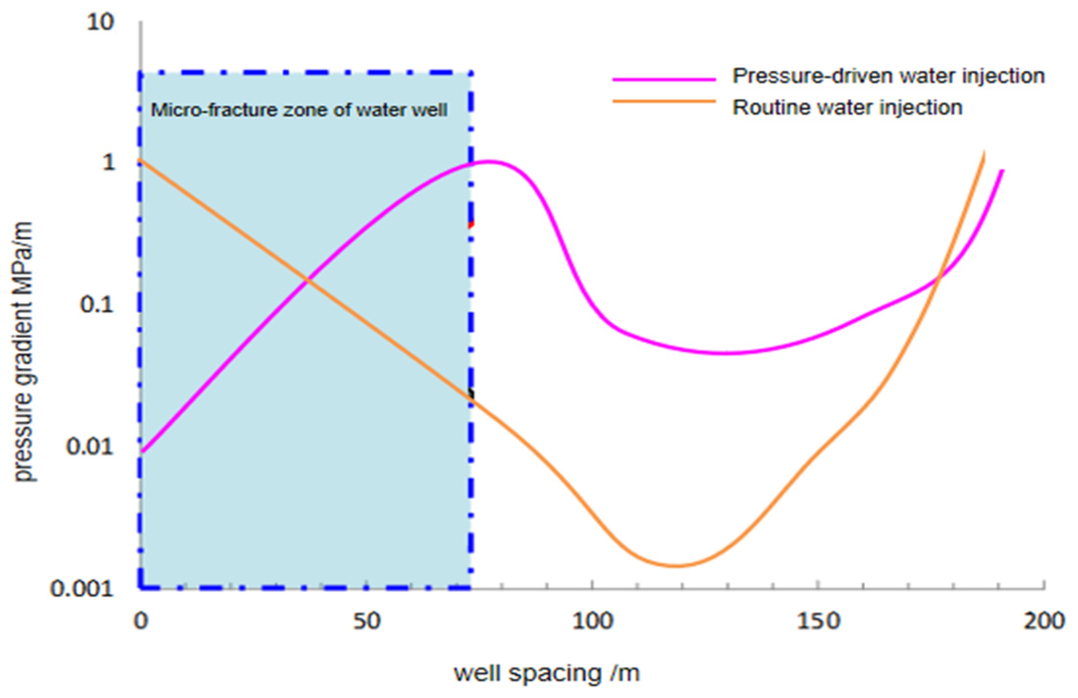
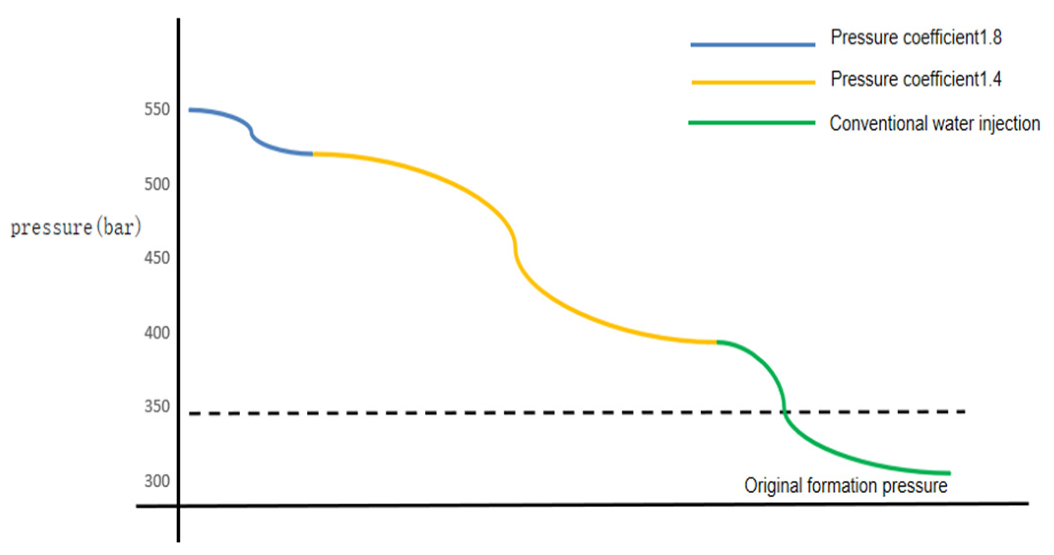
3.1. High Pressure Coefficient: The Key to Establishing a Stable and Continuous Pressure Profile for Long-Term Stable Production

The pressure-driven development of low-permeability reservoirs can create a complex fracture network through high-pressure fluid loss, significantly enhancing permeability and injection capacity for rapid energy replenishment. Compared to conventional water injection, the water injection capacity improves by 10–30 times after pressure-driven water injection. In the pressure-driven modification zone, the pressure front advances, increasing the displacement pressure gradient between wells by 5 to 10 times. Consequently, the range of easily flowing zones expands by 3 to 5 times (Figure 2), enabling the establishment of effective displacement between injection and production wells.
Figure 2 is a comparison of pressure gradient profiles between conventional water injection and pressure-driven water injection. As can be seen from the figure, when the well spacing reaches 80 m, the pressure head moves forward by 800 m, and at this point, the pressure gradient increases by 60 times. This indicates that at this specific well spacing, pressure-driven water injection can significantly improve the pressure gradient, which may enhance the development effect of the reservoir.
There are several reasons for this:
(1)
Fluid dynamics effect: As the well spacing increases, the flow path of the fluid becomes longer, leading to an increase in fluid resistance. In this case, using pressure-driven water injection can overcome this resistance, allowing the fluid to pass through the formation more effectively.
(2)
Influence of microfracture zones: In the area of microfracture zones between wells, the permeability of the formation will change. Pressure-driven water injection can activate these microfractures by increasing the injection pressure, thereby further improving the fluid flow capacity.
(3)
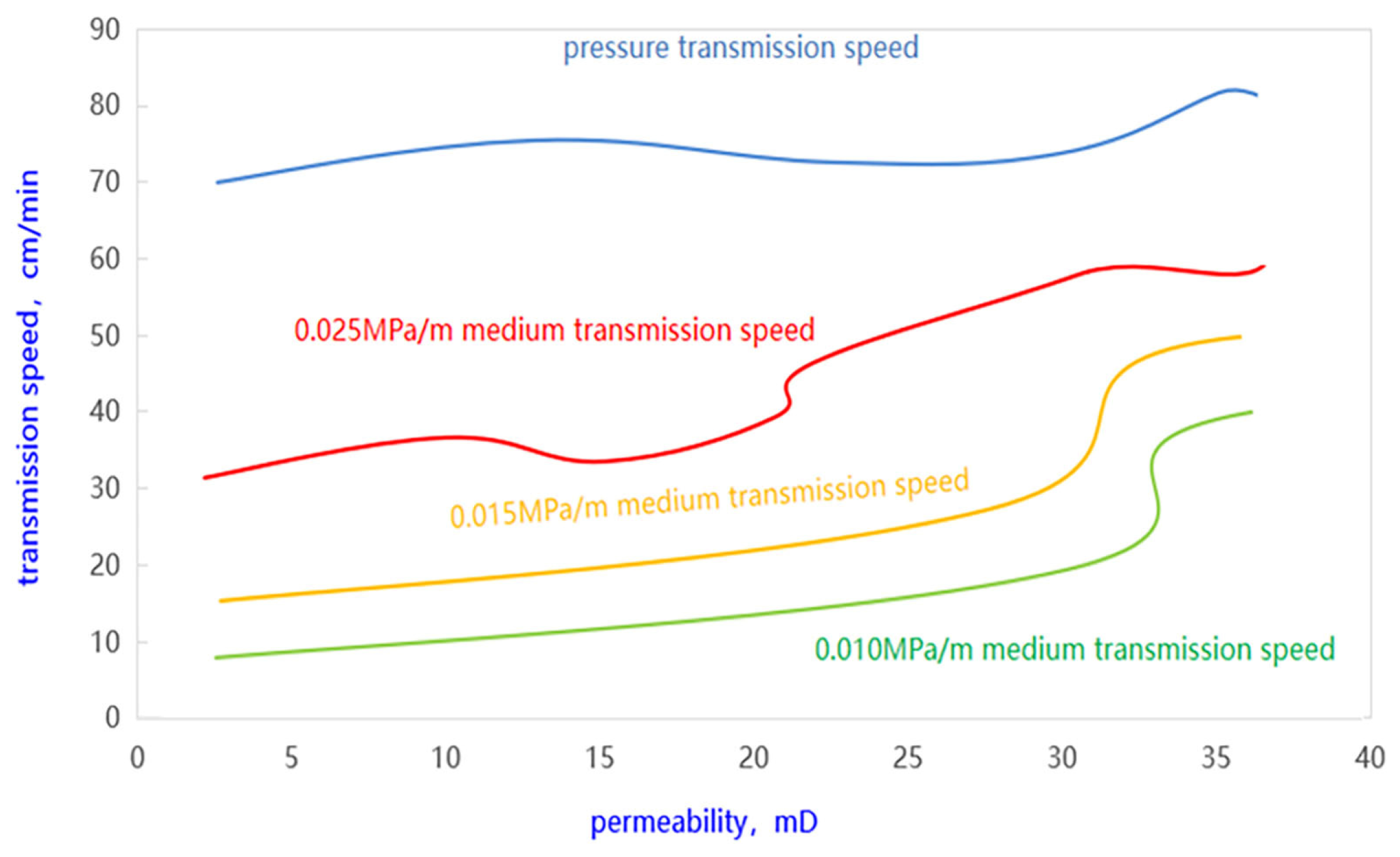
Influence of matrix properties: Factors such as matrix permeability and well spacing may affect the change in pressure gradient. Higher matrix permeability may make it easier for fluids to flow through the formation, while longer well spacing may require higher pressure to maintain the same flow rate.
In the actual oilfield development process, engineers typically determine the best water injection strategy based on field test data and experience. The effect of pressure-driven water injection within this range has been verified through multiple experiments and practical applications.
Our proprietary long-core pressure transmission experiments have demonstrated that the pressure transmission velocity is solely correlated with reservoir physical properties. In contrast, the medium transmission velocity is influenced by both physical properties and pressure gradients. Enhancing physical properties and displacement pressure gradients can reduce the discrepancy between these two velocities.
Pressure transmission refers to the energy transfer resulting from fluid and matrix compression, which is solely related to rock properties and the comprehensive compressibility coefficient of the reservoir. The calculation formula for pressure transmission is:
η = k μ 1 ϕ C t
  • η: Pressure Transmission Coefficient.
  • k: Permeability, with units expressed in Darcies (Darcy, darcies) or millidarcies (mD).
  • μ: Dynamic Viscosity, quantified in units of Pascal-seconds (Pa·s) or centipoise (cP), where 1 Pa·s is equivalent to 1000 cP.
  • φ: Porosity, which represents the ratio of pore space to the total volume, is a dimensionless value ranging from 0 to 1.
  • Ct: Total compressibility factor, encompassing the compressibility of both the fluid and the rock matrix, measured in units of reciprocal Pascals (1/Pa).
Medium transmission refers to the mass transfer caused by fluid migration, which is solely related to rock properties, fluid properties, and displacement pressure gradients. The calculation formula for medium transmission is:
v = k μ Δ p L
  • K: Permeability, units: Darcy (Darcy, darcies) or millidarcies (millidarcies, mD).
  • μ: Dynamic Viscosity, units: Pascal-seconds (Pa·s) or centipoise (centipoise, cP), where 1 Pa·s = 1000 cP.
  • Δp: Pressure Gradient, units: Pascals (Pa) or bars (bar), where 1 bar ≈ 100,000 Pa.
  • v: Fluid Flow Velocity, units: meters per second (m/s) or other velocity units.
  • L: Medium length, meters (m).
Physical simulation experiments on pressure transmission and medium transmission indicate that the lower the reservoir permeability, the greater the discrepancy between the pressure transmission velocity and the medium transmission velocity (Figure 3). When the permeability increases from 5 × 10⁻³ μm2 to 35 × 10−3 μm2, the pressure transmission velocity increases from 70 cm/min to 80 cm/min, a mere increase of 10 cm/min. However, under a pressure gradient of 0.025 MPa/m, the medium transmission velocity increases from approximately 20 cm/min to 50 cm/min. At a pressure gradient of 0.015 MPa/m, the medium transmission velocity rises from around 5 cm/min to 35 cm/min, and under a pressure gradient of 0.01 MPa/m, it increases from approximately 2 cm/min to 25 cm/min. Furthermore, the lower the reservoir permeability, the more significant the discrepancy between the pressure transmission velocity and the medium transmission velocity becomes.
Field practice in pressure-driven oil recovery demonstrates that under conditions of high pressure coefficients, the oil pressure drop rates of both oil and water wells are essentially the same, maintaining a relatively constant injection–production pressure differential. This is conducive to establishing a continuous and stable pressure profile, resulting in a relatively high initial production, a long natural flow period, and minimal decline.
Continuous Pressure Transmission Type: After the first phase of pressure-driven water injection in D-1, the pressure coefficient reached 1.8, with an initial daily oil production of 10.4 t/d. The natural flow period has been prolonged (>220 days) and is still ongoing without any decline. The oil pressure drop rate of the water well is 0.07 MPa/d, while that of the oil well is 0.1 MPa/d (Figure 4a, Continuous Pressure Transmission Type).
Unstable Pressure Transmission Type: After pressure-driven water injection in Block E-1, the pressure coefficient reached 1.3, with an initial daily oil production of 7.3 t/d. However, the natural flow period was short (62 days), followed by a monthly decline rate of 14.5% after flowback and 15.2% after switching to pumping, indicating a significant decline. The oil pressure drop rate of the water well was 0.04 MPa/d, while that of the oil well was 0.2 MPa/d (Figure 4b. Unstable Pressure Transmission Type).
Numerical simulation studies on fluid–solid coupling in pressure-driven oil reservoirs have shown that a high pressure coefficient can ensure stable pressure fronts, enhance the displacement pressure gradient, and facilitate the establishment of a stable and continuous pressure profile (Figure 5). The numerical simulation of the pressure-driven reservoir indicates that a high pressure coefficient ensures a stable pressure head, increases the displacement pressure gradient, and is beneficial for the establishment of a stable and continuous pressure profile. The advanced pressure drive forms a continuous pressure profile between the oil and water wells. Moreover, the high-pressure system can achieve high and stable production with long-term natural flow. Therefore, three regions will form: (1) In the natural flow zone (blue line), the pressure transmission profile is stable, with continuous natural flow; (2) In the stable pumping zone (yellow line), the displacement pressure is stably established, and the pumping maintains certain production capacity; (3) In the depletion decline zone (green line), near the original reservoir pressure, the production declines rapidly, with no period of natural flow.
Based on the above research, it is concluded that a high-pressure system can achieve long-term high and stable production with continuous natural flow.

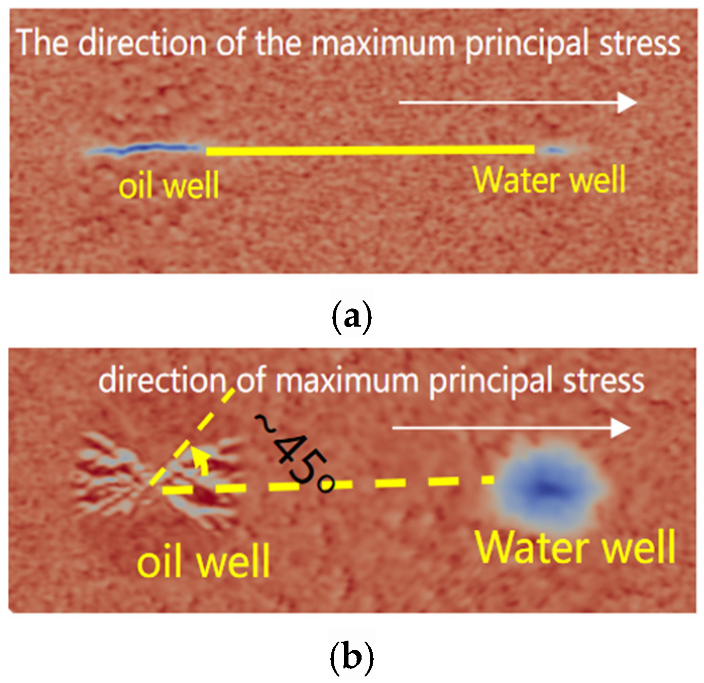
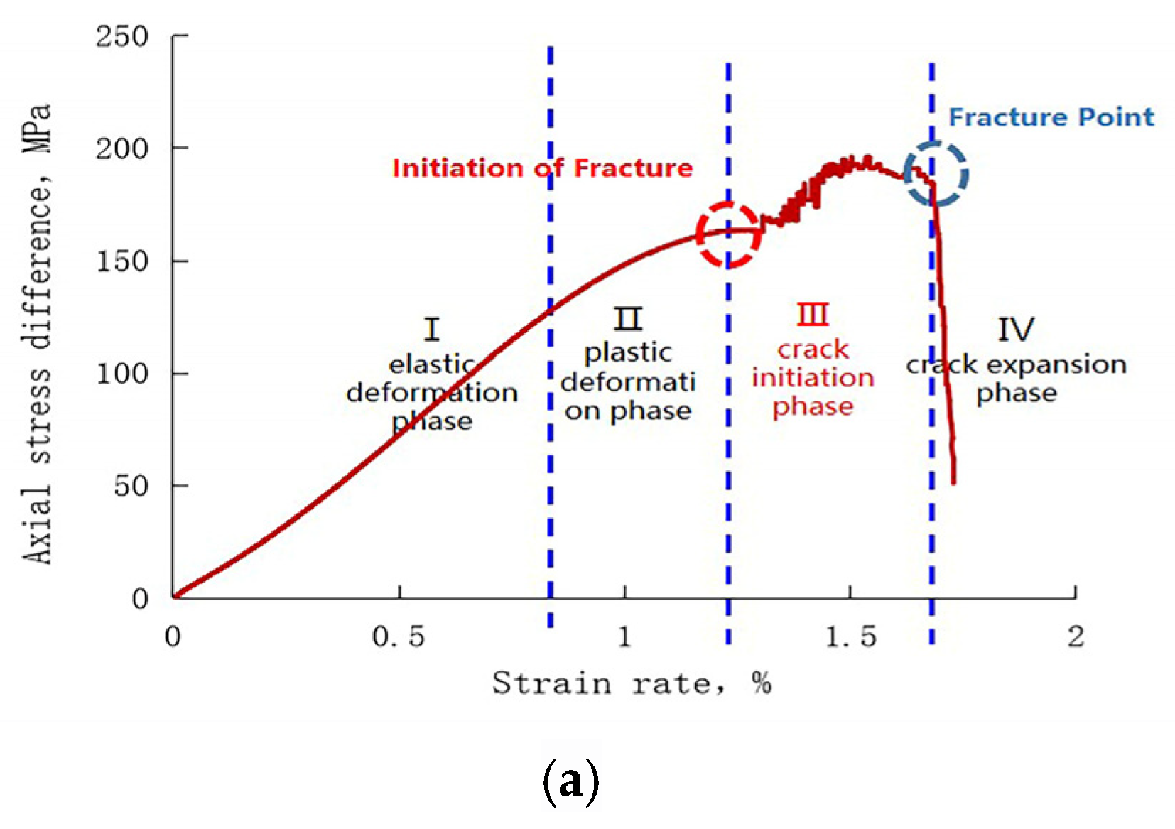
3.2. Sequential Pressure Drive Followed by Fracturing Facilitates the Formation of Complex Redirected Fracture Networks

Physical simulations indicate that high pore pressure reduces the compressive strength of rocks, making reservoirs more susceptible to fracturing. Higher reservoir pressure coefficients lead to lower rock fracture pressures, favoring the development of complex fracture networks. When water injection wells undergo pressure drive prior to fracturing oil wells, the stress field changes, resulting in the formation of redirected fractures.
A high pressure coefficient can ensure a stable pressure front, enhance the displacement pressure gradient, and help establish a continuous pressure profile. When a water injection well is pressure driven before fracturing an oil well, it can cause changes in the stress field. This change may cause the pressure front to become unstable. So, after regular water injection, sudden pressure changes can lead to an unstable pressure head, which in turn affects pressure distribution and causes a decrease. In addition, high pore pressure reduces the compressive strength of rocks, making reservoirs more prone to fracture and forming complex fracture networks. This further affects the propagation and distribution of pressure, leading to instability of the pressure front.
Rock mechanics failure experiments on cores from Block E-1-2 under varying pore pressures reveal that increased pore pressure decreases compressive strength. When the pore pressure is 10 MPa, the rock fracture strain variation rate is approximately 1.0, with an axial stress difference of around 100 MPa. At a pore pressure of 30 MPa, the rock fracture strain variation rate decreases to approximately 0.5, with an axial stress difference of approximately 25 MPa (Figure 6).
Fracture strength experiments on cores from Block E-1-2 under varying pressure coefficients demonstrate that higher pressure coefficients result in lower fracture pressures. At a pressure coefficient of 1.2, the core fracture pressure is 104.8 MPa; at 1.5, it decreases to 92.9 MPa; and at 1.8, it drops further to 30 MPa (Figure 7).
In the instance where the lithostatic ratio (LSR) is 1.2, the reduction in the fracturing pressure of the rock to 30 MPa is attributable to several factors:
(1)
Influence of Pore Pressure: The increase in pore pressure leads to a decrement in the compressive strength of the rock, rendering it more susceptible to fracturing. This is corroborated by Figure 6, wherein the stress differential curves under varying pore pressures illustrate a progressive decline in the rock’s load-bearing capacity as pore pressure intensifies.
(2)
Variations in Formation Stress: The alteration of the lithostatic ratio impacts the effective stress state of the formation. When the formation is under-compacted (with a lithostatic ratio less than 1), the rock may exhibit higher compressive strength; conversely, as the lithostatic ratio approaches or exceeds unity, the increment in pore fluid pressure results in a reduction in the rock’s effective stress, thereby diminishing its resistance to fracturing.
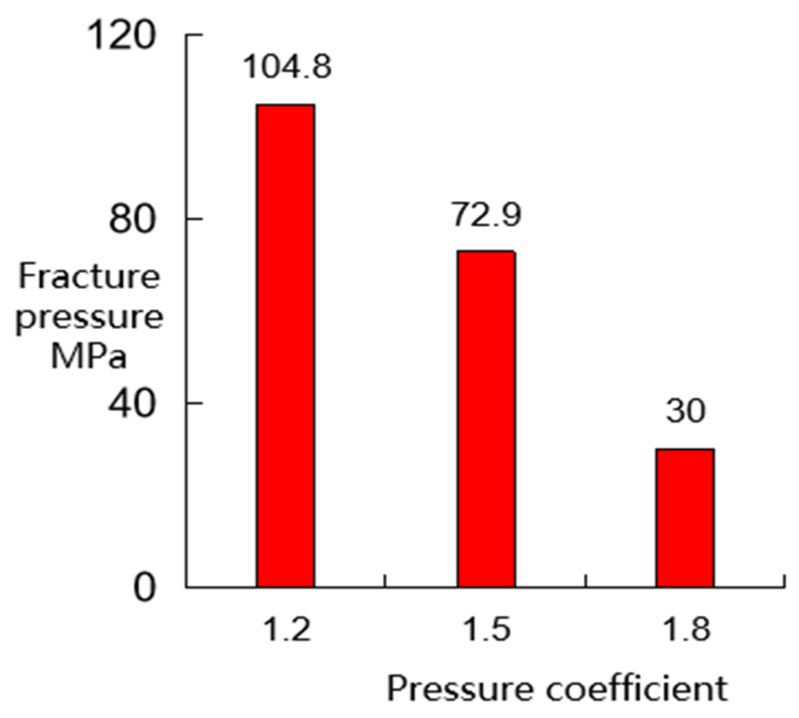
(3)
Support from Physical Simulation Experimentation: The relationship between the lithostatic ratio and fracturing pressure depicted in Figure 8 further endorses this perspective. As the lithostatic ratio increases from 1.0 to 1.8, a marked decrease in the rock’s fracturing pressure is observed, with a significant drop to 72.9 MPa at a lithostatic ratio of 1.5, and a further decline to 30 MPa when the ratio is 1.2.
The decrease in fracturing pressure to 30 MPa at a lithostatic ratio of 1.2 is attributed to the augmentation of pore pressure, which precipitates a decline in the rock’s compressive strength, concurrently with the pivotal role played by changes in formation stress. These findings are substantiated by the results of physical simulation experiments and are in alignment with actual field production scenarios in oil and gas operations.
Numerical simulations of firstly fracturing an oil well followed by pressure drive of a water well indicate that when an oil well is fractured and put into production while maintaining a formation pressure coefficient of 1.0, subsequent pressure drive of the water well tends to induce the formation of long fractures in the oil well that are parallel to the principal stress direction, creating wings on both sides (Figure 8a. Oil wells are fractured first, followed by pressure drive for water wells).
Physical experiments involving water well pressure drive preceding oil well fracturing demonstrate that when the water well undergoes water injection and pressure drive two months in advance, resulting in a formation pressure coefficient reaching 1.8, subsequent fracturing of the oil well leads to the formation of complex fractures, with fracture directions deflecting by approximately 45° (Figure 8b. Water wells undergo pressure drive first, followed by fracturing for oil wells).
Field practice has shown that when fracturing precedes pressure drive, rapid water breakthrough occurs in some oil wells. Adjusting the sequence of production and injection, i.e., performing pressure drive before fracturing, can effectively control water breakthrough.
In Block A-1, the water injection well was fractured prior to the pressure-driven enhancement of the oil well, resulting in rapid water breakthrough in the oil well. In December 2018, well A-1-1 in this block was fractured with two stages, each having a half-length of 122 m. In January 2021, generalized pressure-driven water injection was performed in the water injection well of this block, with a total cumulative water injection volume of 3.7 × 10⁴ m3. Following the pressure-driven water injection, the water cut in well A-1-1, aligned with the principal stress direction, increased rapidly, leading to swift water breakthrough in the oil wells in that same direction (Figure 9).
In Block Bin 435, water wells were initially subjected to pressure-driven injection prior to fracturing the oil wells, leading to a low water cut and a gradual increase in water cut for the oil wells. In January 2023, the water wells in this block underwent staged pressure-driven injection, with a total cumulative water injection volume of 9.6 × 10⁴ m3. By April 2023, the oil wells were brought into production following staged fracturing, which included three fracture stages and a half-fracture length of 157 m. After production commenced, the water cut remained stable, with a slow increase observed (Figure 10).
In Block B-1, the water injection well underwent pressure-driven treatment prior to the fracturing of the oil well, resulting in a low water cut and a gradual increase in the oil well’s water cut. In January 2023, the water injection well in this block experienced staged pressure-driven water injection, with a total cumulative volume of 9.6 × 10⁴ m3. In April 2023, the oil well was brought into production following staged fracturing, which included three fracture stages and a half-fracture length of 157 m. After production commenced, the water cut remained stable and increased slowly (Figure 10).

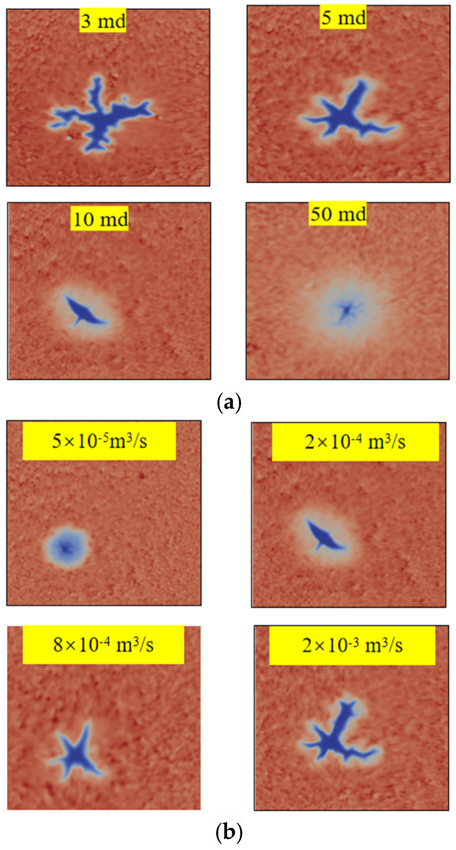
3.3. Reservoir Physical Properties and Injection Displacement Are the Main Controlling Factors Affecting the Morphology and Extension Range of Fracture Network

Physical experiments indicate that the rock-breaking mechanisms vary among reservoirs with different physical properties. Generally, fractures induced by pressure drive in low-permeability reservoirs form during the fracture initiation stage, whereas those in ultra-low-permeability reservoirs occur during the fracture propagation stage after rupture. The distinct stages lead to differences in the morphology and scale of pressure-driven fractures in reservoirs with varying physical properties.
Specifically, when the brittleness index is 2.71 and the gas-measured permeability is 16.0 × 10⁻³ μm2, pressure-driven fractures are generated during the fracture initiation stage (Figure 11a. Brittleness Index: 2.71 Gas Logging Permeability: 16.0 mD).
When the brittleness index is 59.7 and the gas-measured permeability is 3.58 × 10⁻³ μm2, pressure-driven fractures emerge during the fracture propagation stage following rupture (Figure 11b. Brittleness Index: 59.7 Gas Logging Permeability: 3.58 mD).
With a brittleness index of 88.4 and a gas-measured permeability of 0.871 × 10⁻³ μm2, pressure-driven fractures are generated during the fracture propagation stage subsequent to rupture (Figure 11c. Brittleness Index: 88.4 Gas Logging Permeability: 0.87 mD).
Numerical simulations indicate that higher permeability leads to shorter fracture propagation distances and more uniform fracture patterns, while higher injection rates result in longer fracture propagation distances and less uniform fracture patterns. Therefore, to achieve precise control over fracture morphology and propagation distance, it is necessary to match different injection rates with varying reservoir properties.
The schematic diagram of pressure-driven fracture propagation under different perms, with an injection rate of 2 × 10⁻⁴ m3/s and a cumulative injection volume of 0.1 PV, is presented as follows:
When the permeability is 3 × 10⁻³ μm2, the fracture propagation distance is the longest, with fractures extending in all directions. In contrast, when the permeability is 50 × 10−3 μm2, the fracture propagation distance is the shortest, resulting in a more uniform fracture pattern (Figure 12a. Fracture network formed by pressure drive in reservoirs with different physical properties).
With a permeability of 10 × 10−3 μm2 and a cumulative injection volume of 0.1 PV, the schematic diagram of pressure-driven fracture propagation under different injection rates is shown below:
When the injection rate is 2 × 10⁻³ m3/s, the fracture propagation distance is the longest, with fractures extending in all directions. Conversely, at an injection rate of 5 × 10⁻⁵ m3/s, the fracture propagation distance is the shortest, leading to a more uniform fracture pattern (Figure 12b. Fracture network formed by pressure drive in reservoirs with different physical properties).
By implementing advanced high-pressure drive with large well spacing in water wells, we reduced pressure sensitivity and friction, thereby addressing the challenge of inefficient production in low-abundance beach-bar sand reservoirs. Based on the different physical properties of oil layers, we innovatively established a three-dimensional pressure drive approach, optimizing different injection rates to control the propagation morphology of pressure-driven fractures. This achieved high-pressure fluid loss and fracture network creation, resolving the issue of interlayer production differences in ultra-low-permeability reservoirs. Through differential energy replenishment, response induction, displacement adjustment, and flooding, we achieved a synergistic and uniform displacement in the energy field, overcoming the problems of poor sweep efficiency and low recovery rates in conventional low-permeability reservoirs. The in-depth study of pressure drive mechanisms provides guidance for expanding the technical model of pressure drive development in low-permeability reservoirs.

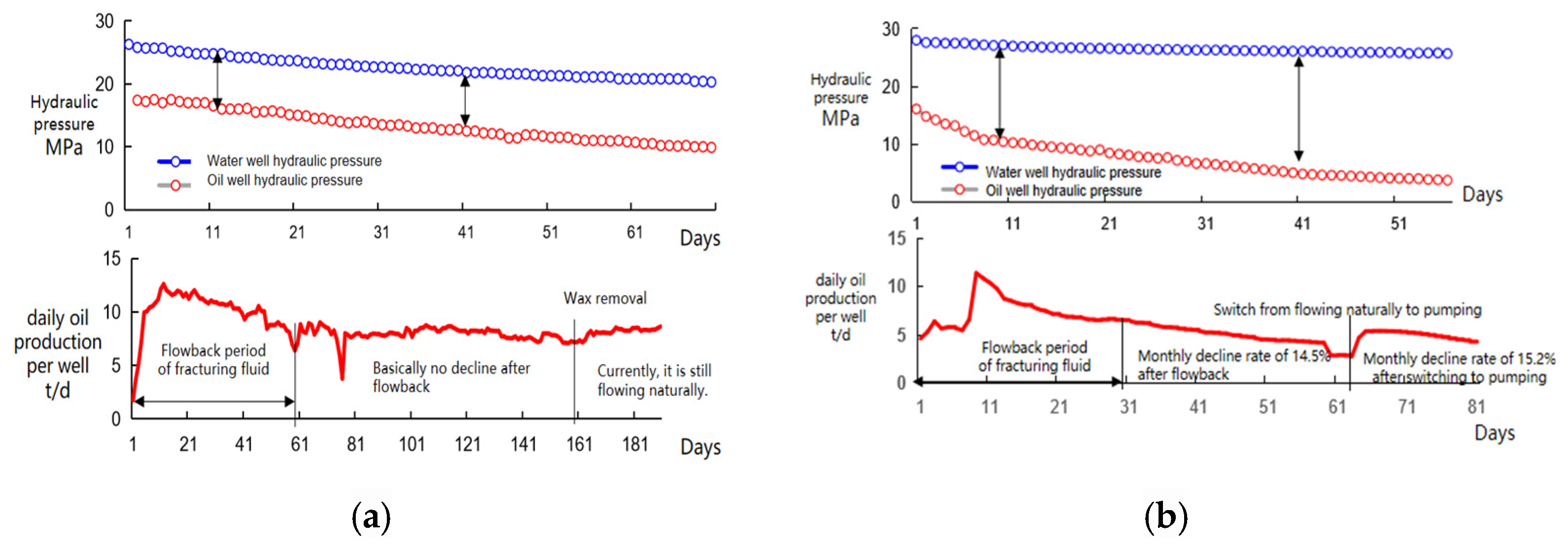
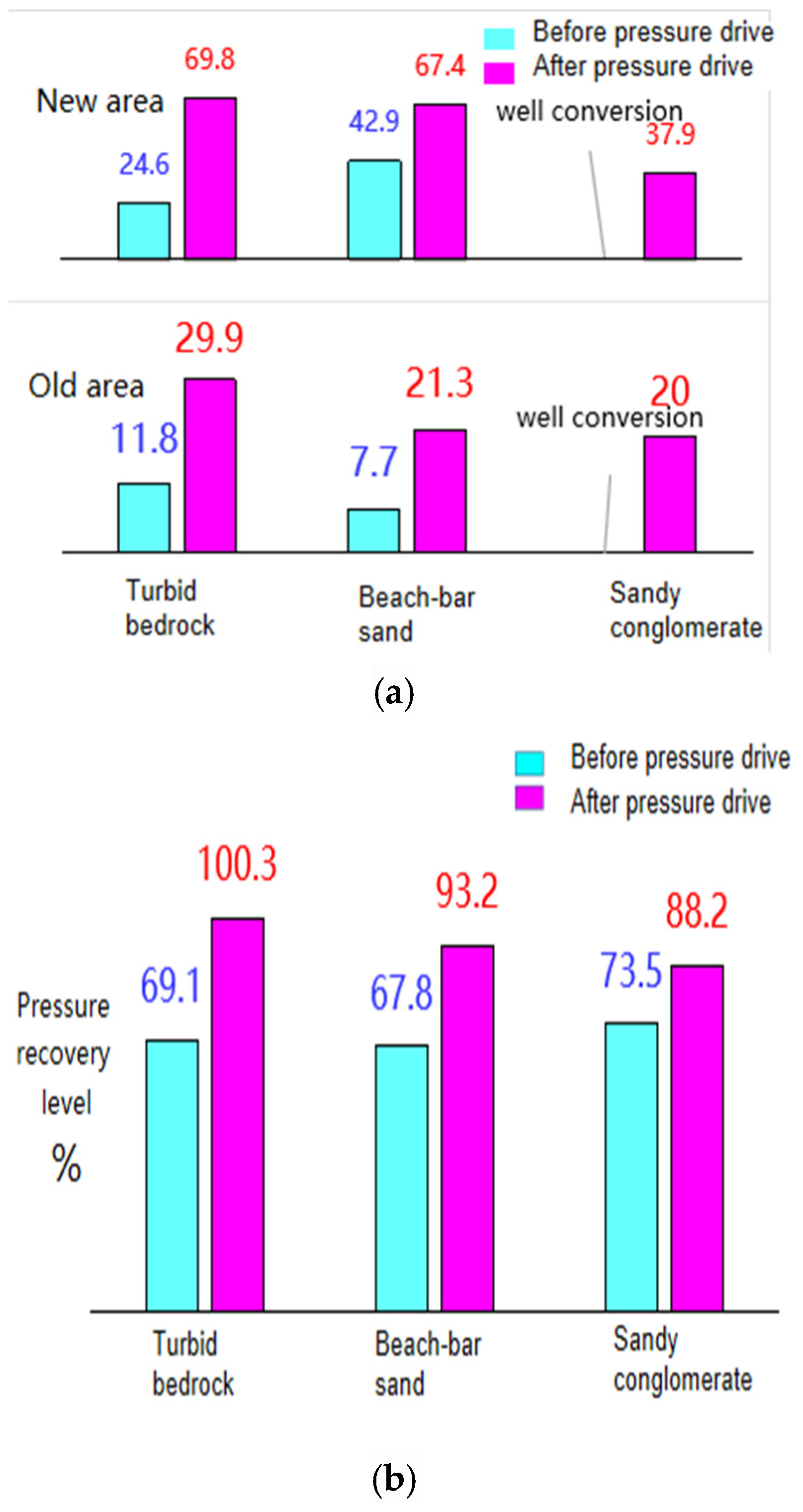
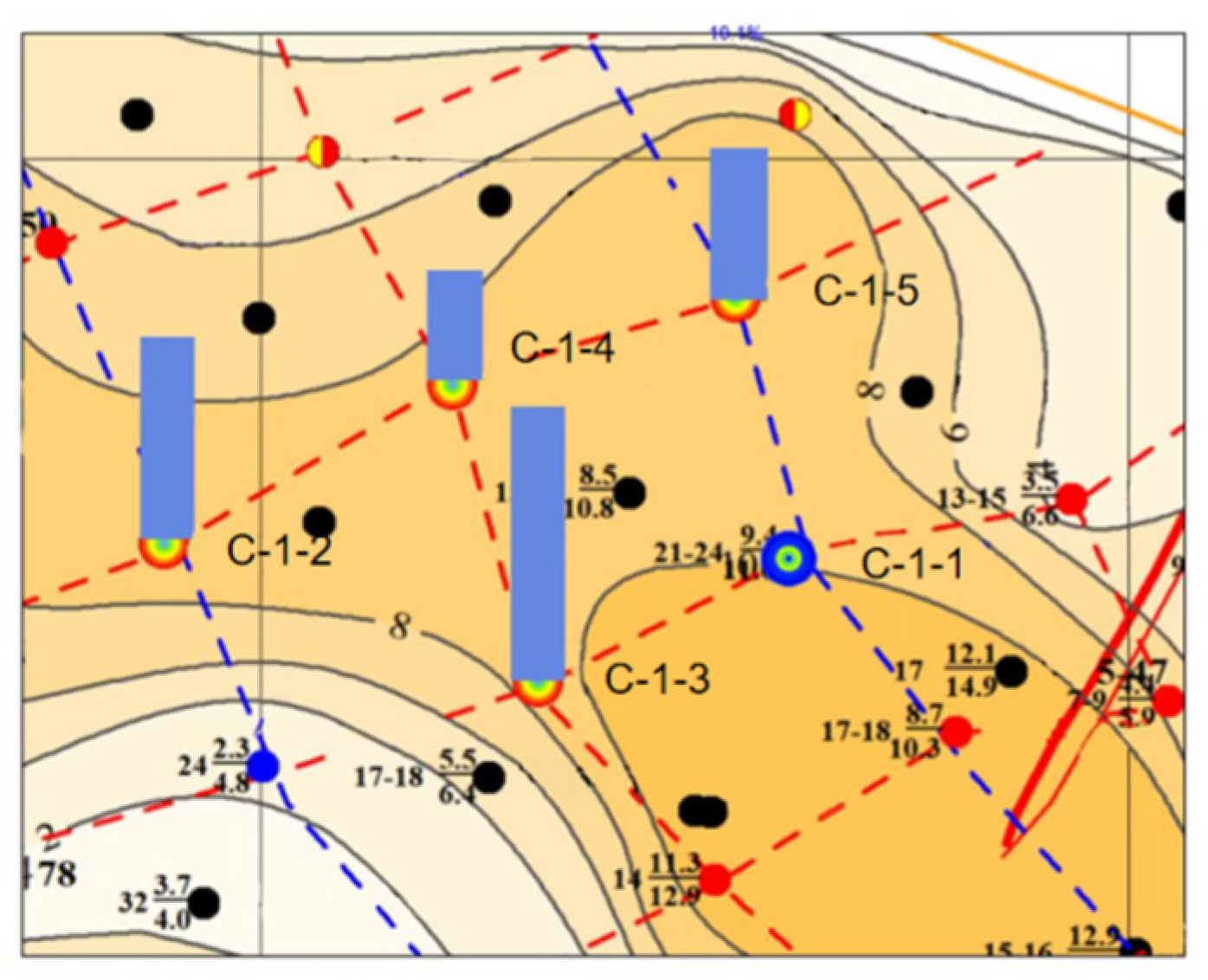
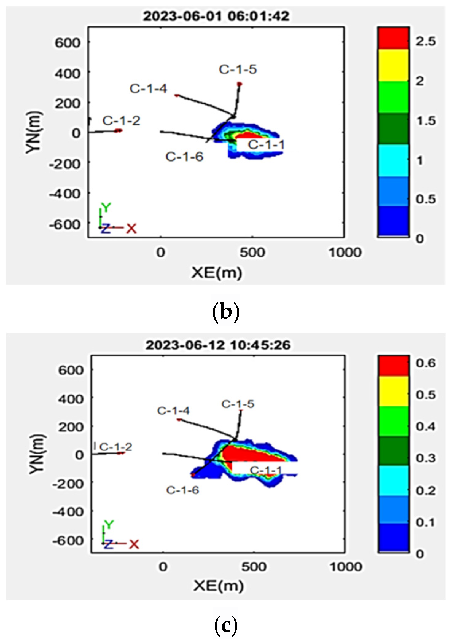
4. Research on Production Characteristics of Pressure Drive in Field Operations

Subsequently, we conducted research on the production characteristics of pressure drive in field operations. Following pressure drive implementation, the daily injection rate per well increased by more than two times, effectively solving the problem of “injection difficulty”. The formation pressure maintenance level rose from 69.3% to 95.7%, effectively restoring formation energy. The fluid production capacity of different types of reservoirs improved by more than 1.2 times, addressing the challenge of “production difficulty”.
We divided the regions into old and new areas, with the previously studied region designated as the old area and the newly developed one as the new area. Pressure drive effectively overcame the “injection difficulty” issue. In the new area, after pressure drive, the water injection capacity of turbidite rocks increased from 24.6 m3/d to 69.8 m3/d, and that of beach-bar sands increased from 42.9 m3/d to 67.4 m3/d. The daily water injection capacity after oil well conversion reached 37.9 m3/d, with a more than two-fold increase compared to pre-pressure drive levels, and a greater improvement observed in turbidite rocks than in beach-bar sands (Figure 13).
In the old area, after pressure drive, the water injection capacity of turbidite rocks increased from 11.8 m3/d to 29.9 m3/d, and that of beach-bar sands increased from 7.7 m3/d to 21.3 m3/d. The daily water injection capacity after oil well conversion reached 20 m3/d, also with a more than two-fold increase compared to pre-pressure drive levels, and a greater improvement in turbidite rocks than in beach-bar sands (Figure 13a. Effect diagram of single-well daily injection increased by more than 2 times compared to before pressure driving).
Pressure drive effectively restored formation energy, with notable improvements in pressure maintenance levels across different rock types. Specifically, for turbidite rocks, the pressure maintenance level increased from 69.1% prior to pressure drive to 100.3% post-pressure drive. Similarly, in beach-bar sands, the pressure maintenance level rose from 67.8% before pressure drive to 93.2% after the process. For conglomerates, the pressure maintenance level improved from 73.5% pre-pressure drive to 88.2% post-pressure drive. On average, the pressure maintenance level across all rock types increased from 69.3% before pressure drive to 95.7% afterward, with turbidite rocks exhibiting the highest pressure recovery level, followed by beach-bar sands, and then conglomerates (Figure 13b. Effect diagram showing a pressure maintenance level of 69.3% before pressure driving and recovery to 95.7% after pressure driving).
Pressure drive addressed the challenge of “inadequate production”. In the new area, the daily fluid production of turbidite rocks increased from 6.9 t/d before pressure drive to a peak of 8.8 t/d afterward, currently stabilizing at 7.6 t/d. For beach-bar sands, daily fluid production rose from 8.8 t/d pre-pressure drive to a peak of 17.0 t/d post-pressure drive, currently at 8.5 t/d. In conglomerates, daily fluid production increased from 10.0 t/d before pressure drive to a peak of 17.1 t/d afterward, currently averaging 13.8 t/d. These data indicate that turbidite rocks and conglomerates maintained relatively stable fluid production post-pressure drive, while beach-bar sands experienced a sharper increase and subsequent decline (Figure 13c. Effect diagram showing liquid production capacity increased by more than 1.2 times for different types of reservoirs).
In the old area, the daily fluid production of turbidite rocks rose from 4.3 t/d before pressure drive to a peak of 7.0 t/d afterward, currently at 5.7 t/d. For beach-bar sands, daily fluid production increased from 4.6 t/d pre-pressure drive to a peak of 8.0 t/d post-pressure drive, currently stabilizing at 4.8 t/d. In conglomerates, daily fluid production rose from 3.0 t/d before pressure drive to a peak of 3.8 t/d afterward, currently averaging 3.5 t/d. These observations suggest that turbidite rocks and conglomerates in the old area also maintained good fluid production capacity post-pressure drive, while beach-bar sands once again demonstrated a steeper increase followed by a quicker decline (Figure 13c. Effect diagram showing liquid production capacity increased by more than 1.2 times for different types of reservoirs).

5. Identify the Main Controlling Factors of Pressure-Driven Technology

In view of the differences in the effects of pressure drive, retrospective evaluations of the main controlling factors of pressure drive in new and old areas are conducted using big data analysis methods such as SHAP analysis and correlation analysis.
The SHAP values for the influencing factors on the effectiveness of pressure drive in the new area are as follows: water injection volume during pressure drive has a SHAP value of 1.1, injection–production well spacing has a SHAP value of 1.08, injection rate has a SHAP value of 0.9, original formation pressure has a SHAP value of 0.66, permeability has a SHAP value of 0.55, reservoir thickness has a SHAP value of 0.3, mid-depth of the reservoir has a SHAP value of 0.22, porosity has a SHAP value of 0.2, and crude oil viscosity has a SHAP value of 0.04 (Figure 14a. SHAP Values for Factors Influencing the Effectiveness of the New Area).
Factors Influencing Cumulative Oil Increment in the New Area and Their Correlation Coefficients:
The correlation coefficients for factors influencing cumulative oil increment in the new area are: water injection volume during pressure drive (0.45), injection–production well spacing (0.43), injection rate (0.40), original formation pressure (0.18), permeability (0.31), reservoir thickness (0.15), mid-depth of the reservoir (0.02), porosity (0.01), and crude oil viscosity (0.02) (Figure 14b Correlation Coefficients of Factors Influencing Cumulative Oil Increment in the New Area).
According to the SHAP values of the influencing factors of the effectiveness status in the new area and the correlation coefficient values of the influencing factors of cumulative oil increase in the new area, the impact values of the main controlling factors of pressure-driven technology in the new area, from largest to smallest, are: pressure-driven water injection volume > injection–production well spacing > injection rate.
SHAP Values for Factors Influencing Effectiveness in the Old Area:
The SHAP values for factors influencing the effectiveness of pressure drive in the old area are: depletion level (1.1), water injection volume during pressure drive (0.9), injection–production well spacing (0.72), injection rate (0.65), permeability (0.36), depleted volume (0.3), water cut before pressure drive (0.28), cumulative injection before pressure drive (0.25), original formation pressure (0.25), mid-depth of the reservoir (0.24), reservoir thickness (0.18), porosity (0.18), and crude oil viscosity (0.11) (Figure 14c. SHAP Values for Factors Influencing the Effectiveness of the Mature Area).
Correlation Coefficients for Cumulative Oil Increment in the Old Area:
The correlation coefficients for factors influencing cumulative oil increment in the old area are: depletion level (0.61), water injection volume during pressure drive (0.53), injection–production well spacing (0.50), injection rate (0.33), permeability (0.33), reservoir thickness (0.28), depleted volume (0.25), water cut before pressure drive (0.13), cumulative injection before pressure drive (0.14), original formation pressure (0.13), mid-depth of the reservoir (0.12), porosity (0.08), and crude oil (0.01) (Figure 14d. Correlation Coefficients of Factors Influencing Cumulative Oil Increment in the Mature Area Contributions).
Based on the SHAP values of the influencing factors of the effectiveness status in the old area and the correlation coefficient values of the influencing factors of cumulative oil increase in the old area, the impact values of the main controlling factors of pressure-driven technology in the old area, from largest to smallest, are: degree of depletion > pressure-driven water injection volume > injection–production well spacing.
Oil wells with large depletions are more prone to water breakthrough, and the pressure-driven design in old fields should pay more attention to the imbalance of pressure and flow field caused by historical exploitation. Taking the well group C-1-1 as an example, well C-1-2 in this group has a depletion of 12.1%, well C-1-3 has a depletion of 15.4%, well C-1-4 has a depletion of 7.1%, and well C-1-5 has a depletion of 10.1% (Figure 15). According to the monitoring of the water injection front of well C-1-1, water breakthrough occurred in well C-1-3, which has a larger depletion.
Figure 16 illustrates the changes in the water injection front for Well Group C-1-1 at different time periods, specifically on 24 May 2023, 1 June 2023, and 12 June 2023. As shown in (Figure 16a), the water injection front change on 24 May 2023; in (Figure 16b), the water injection front change on 1 June 2023; and in (Figure 16c), the water injection front change on 12 June 2023.

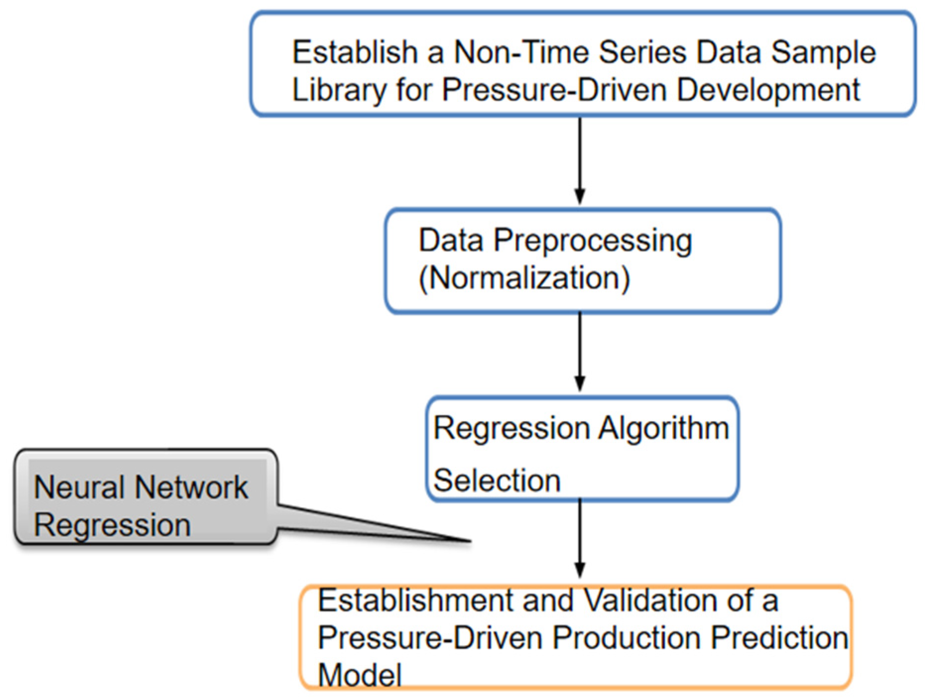
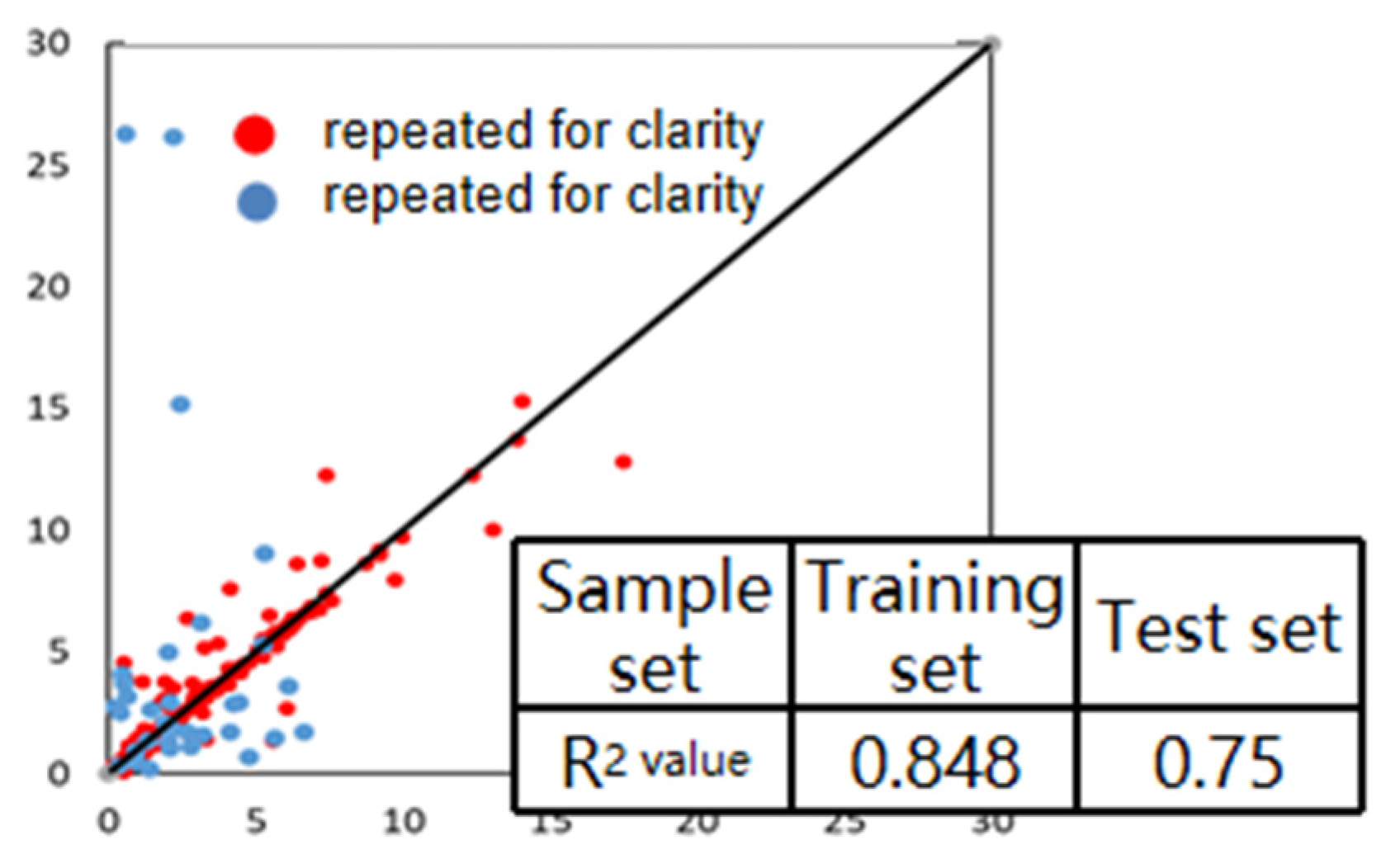
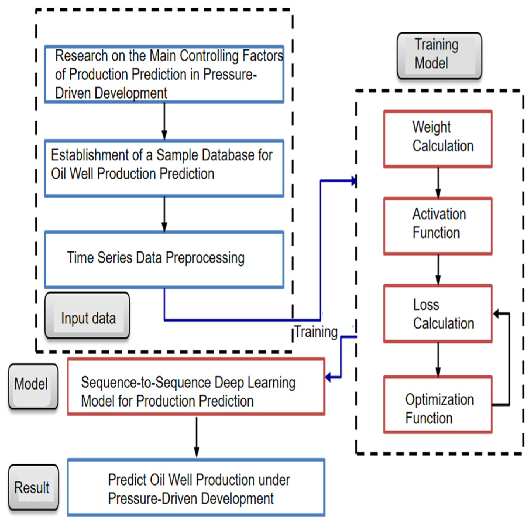
6. Prediction Model for Pressure Drive Effectiveness

A predictive model for pressure drive productivity, both non-time series- and time series-based, has been established utilizing data-driven approaches specific to pressure drive operations. This model aims to forecast the effectiveness of pressure drive measures by leveraging historical and real-time data pertaining to the process.
Flowchart for Establishing and Validating a Pressure-Driven Production Prediction Model with Non-Time-Series Data Sample Libraries, Including Data Preprocessing (Standardization), Selection of Appropriate Regression Algorithms (Figure 17).
In a neural network [41], multiple neurons can be combined to form a layer, and the stacking of these layers creates the network structure. We employ a Multi-Layer Perceptron (MLP).
z ( l ) = f ( W ( l ) a ( l 1 ) + b ( l ) )
where:
  • z(l) represents the activation output of the l $-th layer.
  • W(l) denotes the weight matrix associated with the l $-th layer.
  • a(l) is the activation output of the l-1 layer, which also serves as the input to the l layer.
  • b(l) is the bias vector for the l layer.
Non-time-series pressure-driven production capacity prediction model based on machine learning (neural network regression algorithm), with the neural network fitting diagram for the three months following pressure drive shown above (Figure 18).
Time Series Production Forecast Model Based on Deep Learning:
Based on the established pressure-driven production capacity prediction model, a regression plot for the daily oil production over three months was obtained, as shown in the above figure (Figure 19). A time series production forecast model employing a sequence-to-sequence (seq-seq) deep learning architecture has been developed. This model comprehensively considers not only the temporal influence of production dynamics on output but also the spatial impact of static geological parameters. The flowchart illustrating the model’s framework is presented below (Figure 20). Results from both training and testing phases (Figure 21) demonstrate that the proposed deep learning-based time series production forecast model achieves high accuracy, underscoring its effectiveness in predicting production outcomes.
Time series models for addressing pressure-driven problems can take various forms. We base our approach on the linear autoregressive model (AR) and incorporate pressure as an exogenous input variable. Let Pt denote the pressure at time t, and Xt represent the target variable at time t (e.g., flow rate, head height, etc.) The pressure-driven time series model can be expressed as:
X t = c + i = 1 p ϕ i X t i + θ P t + ε t
where:
  • c is the constant term.
  • ϕi is the coefficient of the autoregressive term, indicating the influence of past values of the target variable on the current value.
  • p is the order of the autoregressive model.
  • θ is the coefficient of the pressure term, representing the impact of pressure on the target variable.
  • Pt is the pressure at the current time.
  • εt is the error term, assumed to be a white noise process with a mean of zero.
This model assumes that the target variable Xt is influenced by its own past values as well as the current pressure Pt. Such a model can be utilized to predict future values of the target variable (including production) given current and past pressure data.

7. Conclusions

This study delves into the exploitation mechanism of pressure drive by establishing mathematical models for oil-water seepage in tight oil reservoirs, a model of fracture permeability, and a prediction model for the pressure drive effect, elucidating the underlying mechanisms of pressure drive technology in enhancing oil recovery (EOR).
(1)
An innovative approach to complex fracture networks was developed by investigating the strategy of pressure drive prior to fracturing, revealing that establishing a stable and continuous pressure profile with a high pressure coefficient is crucial for achieving long-term stable production, and also facilitates the formation of complex and branched fracture networks.
(2)
Based on the varying physical properties of reservoirs, we innovatively developed a three-dimensional pressure drive method, optimizing different injection rates to control the propagation patterns of pressure-driven fractures, ultimately leading to high-pressure leak-off and the creation of complex fracture networks.
(3)
The analysis identifies reservoir physical properties and injection displacement as the main controlling factors affecting the morphology and extension range of the fracture network.
(4)
We conducted field-scale studies on the production characteristics of pressure drive operations, utilizing big data analytic tools such as SHAP analysis and correlation analysis to retrospectively evaluate the primary controlling factors of pressure drive in both new and established fields.
Compared to previous research on oil recovery solutions, the pressure drive method investigated in this study yields more pronounced results. Looking forward, we aim to explore deeper issues, expand our sample range, and experiment with different approaches to further advance our understanding and application of this technology.

Author Contributions

Conceptualization, H.L.; Methodology, B.J.; Validation, B.J.; Formal analysis, H.L.; Investigation, B.J.; Resources, B.J.; Writing—original draft, H.L. All authors have read and agreed to the published version of the manuscript.

Funding

This research was funded by [“Key Technology for Profitable Development of Untapped Reserves in Ultra-Low Permeability Oil Reservoirs” project by Sinopec] grant number [P24021] And The APC was funded by [“Key Technology for Profitable Development of Untapped Reserves in Ultra-Low Permeability Oil Reservoirs” project by Sinopec].

Data Availability Statement

The original contributions presented in the study are included in the article, further inquiries can be directed to the corresponding authors.

Conflicts of Interest

Author Haicheng Liu was employed by the Exploration and Development Research Institute of Sinopec Shengli Oilfield Company. The remaining authors declare that the research was conducted in the absence of any commercial or financial relationships that could be construed as a potential conflict of interest.

References

  1. Qing, L.; Yuan, C.; Qiang, L. Establishment and evaluation of strength criterion for clayey silt hydrate-bearing sediments. Energy Sources Part A Recovery Util. Environ. Eff. 2018, 40, 742–750. [Google Scholar]
  2. Li, Q.; Wang, Y.; Wang, F. Effect of thickener and reservoir parameters on the filtration property of CO2 fracturing fluid. Energy Sources Part A Recovery Util. Environ. Eff. 2019, 42, 1705–1715. [Google Scholar] [CrossRef]
  3. Guo, H.; Cheng, L.; Wang, P.; Jia, P. Water flooding experiment and law of carbonate reservoir cores with different fracture occurrences. Pet. Geol. Recovery Effic. 2022, 29, 105–112. [Google Scholar]
  4. Yi, Z.; Yong, Y.; Zhi, S. Physical simulation of fracturing-flooding and quantitative characterization of fractures in low-permeability oil reservoirs. Pet. Geol. Recovery Effic. 2022, 29, 143–149. [Google Scholar]
  5. Li, C. Principles of Reservoir Engineering; Petroleum Industry Press: Beijing, China, 2011; pp. 190–197. [Google Scholar]
  6. Feng, Z. The Mechanism and Parameters-Optimization of Injection Fracture Pressure Propagation for Low Permeability Oil Field. Ph.D. Thesis, China University of Petroleum, Qingdao, China, 2009. [Google Scholar]
  7. Jie, C.; Bin, J.; Jia, W. A novel numerical simulation of CO2 immiscible flooding coupled with viscosity and starting pressure gradient modeling in ultra-low permeability reservoir. Front. Earth Sci. 2023, 17, 884–898. [Google Scholar]
  8. Jie, C.; Jia, W. A new calculation method on the critical well spacing of CO2 miscible flooding in ultra-low permeability reservoirs. J. Porous Media 2021, 24, 59–79. [Google Scholar]
  9. Guan, Z.; Xiao, X.; Qing, Z. Study on hydraulic fracture propagation mechanism of pore-elastic media based on time-step linear superposition method. Drill. Prod. Technol. 2021, 44, 88–92. [Google Scholar]
  10. Joseph, C.; Figueroa, A.A.; Ignacio, L.J. Self Adjusting Pressure Drive Shaft. Patent US20030226874A1, 11 December 2002. [Google Scholar]
  11. Stines, J.R. Rotational Pressure Drive for a Medical Syringe. Patent US07/960022, 1 March 1994. [Google Scholar]
  12. Pu, C.; Liu, Z.; Pu, G. On the Factors of Impact Pressure in Supercritical CO2 Phase-Transition Blasting—A Numerical Study. Energies 2022, 15, 8599. [Google Scholar] [CrossRef]
  13. Chang, X.; Yong, Z. Analysis of Oil Production and Fracturing Technologies for Low-Permeability Reservoirs. Petrochem. Technol. 2024, 31, 100–102. [Google Scholar]
  14. Ze, R. High-efficient Development of Low-permeability Reservoir with Geology and Engineering Integration: A Case Study of N25 Block in Dongying Sag. Drill. Prod. Technol. 2024, 47, 90–96. [Google Scholar]
  15. Shu, L.; Ding, Z.; Yong, W. Experimental Study on Micro-Nano Emulsion Injection Enhancement Technology for Low-Permeability Reservoirs. Petrochem. Technol. 2024, 53, 553–558. [Google Scholar]
  16. Duo, P. Research on Enhanced Oil Recovery Technologies for Low-Permeability Reservoirs. Petrochem. Technol. 2023, 30, 50–52. [Google Scholar]
  17. Liu, J.; Yao, Y.B.; Elsworth, D. Morphological complexity and azimuthal disorder of evolving pore space in low-maturity oil shale during in-situ thermal upgrading and impacts on permeability. Pet. Sci. 2024, 1, 1–20. [Google Scholar] [CrossRef]
  18. Jin, Y. Fracturing Technology and Development Trends in Low-Permeability Oilfields. China Pet. Chem. Stand. Qual. 2023, 43, 175–177. [Google Scholar]
  19. Yong, Y.; Shi, Z.; Xiao, C. Practice and understanding of pressure drive development technology for low-permeability reservoirs in Shengli Oilfield. Pet. Geol. Recovery Effic. 2023, 30, 61–71. [Google Scholar]
  20. Bai, X.F.; Li, J.H.; Liu, X.; Wang, R.; Ma, S.; Yang, F.; Li, X.; Liu, J. Evolution of the Anisotropic Thermo-physical Performance for LowMaturity Oil Shales at an Elevated Temperature and Its Implications for Re-storing Oil Development. Energy Fuels 2024, 38, 15216–15224. [Google Scholar] [CrossRef]
  21. Zhang, S.Q.; Liu, J.; Li, L.; Kassabi, N.; Hamdi, E. Petrophysical and Geochemical Investigation-Based Methodology for Analysis of the Multilithology of the Permian Longtan Formation in Southeastern Sichuan Basin, SW China. Energies 2024, 17, 766. [Google Scholar] [CrossRef]
  22. Li, L.; Ma, S.; Liu, X.; Liu, J.; Lu, Y.; Zhao, P.; Kassabi, N.; Elsworth, D. Coal measure gas resources matter in China: Review, challenges, and perspective. Phys. Fluids 2024, 36, 071301. [Google Scholar] [CrossRef]
  23. Chuan, C.; Huai, L.; Zhong, W. Analysis of pressures in water injection wells considering fracture influence induced by pressure-drive water injection. Pet. Reserv. Eval. Dev. 2023, 13, 686–694. [Google Scholar]
  24. Yi, L.; Feng, W.; Yu, W. Mechanism of Enhanced Oil Recovery by Pressure Driving in Medium-Low Permeability Reservoirs. Pet. Explor. Dev. 2022, 49, 752–759. [Google Scholar]
  25. Xiao, C. Practice and Understanding of Pressure-Driven Water Injection Technology in Binnan. Inn. Mong. Petrochem. Ind. 2024, 50, 43–46. [Google Scholar]
  26. Feng, W.; He, X.; Yi, L. Mechanism of Enhanced Oil Recovery by Pressure Driving Technology with High Pressure Drop Adsorption. Acta Pet. Sin. 2024, 45, 403–411. [Google Scholar]
  27. Qi, H.; Guo, P.; Yan, L. Pressure-Driven Water Injection Technology and Development Directions for Low-Permeability Reservoirs. Contemp. Petrochem. 2023, 31, 26–29. [Google Scholar]
  28. Liu, Y.; Yamada, Y. The Characteristics and Design of Hybrid Pressure Drive System with Turbofan and Switch Valve for Laminated Foam-based Soft Actuator. In Proceedings of the JSME annual Conference on Robotics and Mechatronics (Robomec), Osaka, Japan, 6–8 June 2021; pp. 2A1–D02. [Google Scholar] [CrossRef]
  29. Chiodini, G.; Paonita, A.; Aiuppa, A. Magmas near the critical degassing pressure drive volcanic unrest towards a critical state. Nat. Commun. 2016, 7, 13712. [Google Scholar] [CrossRef] [PubMed]
  30. Velarde, E.; Ezcurra, E.; Horn, M.H. Warm oceanographic anomalies and fishing pressure drive seabird nesting north. Sci. Adv. 2015, 1, e1400210. [Google Scholar] [CrossRef]
  31. Ishizuka, S.; Hamasaki, T.; Koumura, K. Measurements of flame speeds in combustible vortex rings: Validity of the back-pressure drive flame propagation mechanism. Proc. Symp. Combust 1999, 27, 727–734. [Google Scholar] [CrossRef]
  32. Nakazawa, H.; Yokota, S.; Kita, Y. A Constant Pressure Drive System for Engine-Flywheel Hybrid Vehicles (First Report, Simulations for Fuel Saving Analysis of Hybrid Vehicles Using a Flywheel Pump/motor). J. Jpn. Hydraul. Pneum. Soc. 1996, 27, 513–518. [Google Scholar] [CrossRef]
  33. Zhang, Z.; Xu, S.; Gou, Q.; Li, Q. Reservoir Characteristics and Resource Potential of Marine Shale in South China: A Review. Energies 2022, 15, 8696. [Google Scholar] [CrossRef]
  34. Han, Z.; Dong, M.A.; Hou, B.W. Post-earthquake hydraulic analyses of urban water supply network based on pressure drive demand model. Sci. Sin. Technol. 2019, 49, 351–362. [Google Scholar] [CrossRef]
  35. Jie, C.; JU, B.; Lyu, G. A computational method of critical well spacing of CO2 miscible and immiscible concurrent flooding. Pet. Explor. Dev. Online 2017, 44, 815–823. [Google Scholar]
  36. Jie, C.; Bin, J.; Wen, C. Laboratory simulation of CO2 immiscible gas flooding and characterization of seepage resistance. Front. Earth Sci. 2023, 17, 797–817. [Google Scholar]
  37. Jun, Z.; Peng, Y.; Su, W. 3D numerical simulation of fracture dynamic propagation in hydraulic fracturing of low-permeability reservoir. Acta Pet. Sin. 2010, 31, 119–123. [Google Scholar]
  38. Shuai, T.; Yong, H.; Jie, Z. Reasonable pattern well spacing deployment of lens lithologic reservoirs with low permeability. Lithol. Reserv. 2018, 30, 116–123. [Google Scholar]
  39. Ji, H. Application of advanced water injection inflow production relation model in low-permeability reservoir. Spec. Oil Gas Reserv. 2020, 27, 92–97. [Google Scholar]
  40. Quan, Z.; Ming, L.; Zi, Z. Application of volume fracturing technology in tight oil reservoirs of Shengli oilfield. China Pet. Explor. 2019, 24, 233–240. [Google Scholar]
  41. Song, F.; Ding, H.; Wang, Y.; Zhang, S.; Yu, J. A Well Production Prediction Method of Tight Reservoirs Based on a Hybrid Neural Network. Energies 2023, 16, 2904. [Google Scholar] [CrossRef]
Figure 1. Solution Framework for Pressure Analysis Model of Pressure-Driven Water Injection Wells.
Energies 17 05253 g001
Figure 2. Pressure Gradient Profiles of Conventional Water Injection versus Pressure-Driven Water Injection.
Energies 17 05253 g002
Figure 3. Variation Curves of Pressure and Fluid Transmission Velocity with Permeability.
Energies 17 05253 g003
Figure 4. Variation Curves of Oil Pressure and Daily Oil Production of Oil and Water Wells After Well Opening in Block D-1-1. (a) Continuous Pressure Transmission Type, (b) Unstable Pressure Transmission Type.
Energies 17 05253 g004
Figure 5. Continuous Pressure Profiles between Oil and Water Wells under Different Pressure Coefficients for Advanced Pressure-Driven Injection.
Energies 17 05253 g005
Figure 6. Rock Mechanics Failure Curves of Cores from Block E-1-2 under Different Pore Pressures.
Energies 17 05253 g006
Figure 7. Histogram of Fracture Pressures of Cores from Block E-1-2 under Different Pressure Coefficients.
Energies 17 05253 g007
Figure 8. Schematic Diagram of Fracture Propagation in Oil Wells after Initially Fracturing Water Wells and Subsequently Applying Pressure-Driven Injection to Oil Wells, and Schematic Diagram of Fracture Propagation in Oil Wells after Initially Applying Pressure-Driven Injection to Water Wells and Subsequently Fracturing Oil Wells. (a) Oil wells are fractured first, followed by pressure drive for water wells. (b) Water wells undergo pressure drive first, followed by fracturing for oil wells.
Energies 17 05253 g008
Figure 9. Water Cut Variation Curve of Oil Well A-1-1 in the Direction of Principal Stress (Block A).
Energies 17 05253 g009
Figure 10. Water Cut Variation Curve of Oil Well B-1-1 in the Direction of Principal Stress (Block B).
Energies 17 05253 g010
Figure 11. Strain–stress difference curves at permeabilities of 16.0 × 10⁻³ um2, 3.58 × 10⁻³ um2, and 0.871 × 10⁻³ um2, respectively. (a) Brittleness Index: 2.71 Gas Logging Permeability: 16.0 mD. (b) Brittleness Index: 59.7 Gas Logging Permeability: 3.58 mD. (c) Brittleness Index: 88.4 Gas Logging Permeability: 0.871 mD.
Energies 17 05253 g011aEnergies 17 05253 g011b
Figure 12. Fracture propagation patterns under different permeabilities, and fracture propagation patterns under different injection rates. (a) Fracture network formed by pressure drive in reservoirs with different physical properties. (b) Fracture network formed by pressure drive in reservoirs with different physical properties.
Energies 17 05253 g012
Figure 13. Histogram of Water Injection Capacity after Transition from Pressure-Driven Injection to Conventional Water Injection in Reservoirs of Different Lithologies. (a) Effect diagram of single-well daily injection increased by more than 2 times compared to before pressure driving. (b) Effect diagram showing a pressure maintenance level of 69.3% before pressure driving and recovery to 95.7% after pressure driving. (c) Effect diagram showing liquid production capacity increased by more than 1.2 times for different types of reservoirs.
Energies 17 05253 g013aEnergies 17 05253 g013b
Figure 14. Evaluation of main controlling factors of pressure-driven technology in new and old areas. New area: pressure-driven water injection volume > injection–production well spacing > injection rate; Old area: degree of depletion > pressure-driven water injection volume > injection–production well spacing (data bar chart). (a) SHAP Values for Factors Influencing the Effectiveness of the New Area. (b) Correlation Coefficients of Factors Influencing Cumulative Oil Increment in the New Area. (c) SHAP Values for Factors Influencing the Effectiveness of the Mature Area. (d) Correlation Coefficients of Factors Influencing Cumulative Oil Increment in the Mature Area Contributions.
Energies 17 05253 g014aEnergies 17 05253 g014b
Figure 15. Bar Chart of Oil Well Depletion Degree in Well Group C-1-1.
Energies 17 05253 g015
Figure 16. Variation in Water Injection Front at Different Time Periods in Well Group C-1-1. (a) Water Injection Front Variation Chart on 24 May 2023. (b) Water Injection Front Variation Chart on 1 June 2023. (c) Water Injection Front Variation Chart on 12 June 2023.
Energies 17 05253 g016aEnergies 17 05253 g016b
Figure 17. Flowchart of a Non-Temporal Pressure-Driven Production Prediction Model Based on Machine Learning.
Energies 17 05253 g017
Figure 18. Neural Network Fitting Chart for Three Months After Pressure-Driven Injection.
Energies 17 05253 g018
Figure 19. Regression Chart of Daily Oil Production Model for Three Months.
Energies 17 05253 g019
Figure 20. Time Series Production Prediction Model Based on Deep Learning.
Energies 17 05253 g020
Figure 21. Time Series Production Regression Chart for Deep Learning.
Energies 17 05253 g021
Disclaimer/Publisher’s Note: The statements, opinions and data contained in all publications are solely those of the individual author(s) and contributor(s) and not of MDPI and/or the editor(s). MDPI and/or the editor(s) disclaim responsibility for any injury to people or property resulting from any ideas, methods, instructions or products referred to in the content.

