Article

Proposal of Three Methods for Deriving Representative Mean Radiant Temperatures Considering Zone Spatial Distributions

1
Department of Architecture, Keimyung University, Daegu 42601, Republic of Korea
2
Division of Architecture, Inha University, Incheon 22212, Republic of Korea
3
Department of Architectural Engineering, Keimyung University, Daegu 42601, Republic of Korea
*
Author to whom correspondence should be addressed.
Energies 2024, 17(20), 5221; https://doi.org/10.3390/en17205221
Submission received: 24 September 2024 / Revised: 15 October 2024 / Accepted: 18 October 2024 / Published: 20 October 2024
(This article belongs to the Special Issue Energy Consumption and Environmental Quality in Buildings)

Abstract

:
Mean radiant temperature (MRT), which is a crucial factor for thermal comfort, varies within a space. This renders deriving the representative values for radiant heating and cooling control challenging. This study reviewed existing methods for deriving MRT in previous research and addressed their limitations by proposing a method for determining a representative MRT value. The existing methods were categorized as air temperature, single location, and area weighted. Three methods for deriving representative MRT values were proposed, considering the building’s usage, scale, and applicable system installations. The proposed methods were categorized as single-zone averaged, multi-zone averaged, and point-zone MRT. Experiments were conducted by distinguishing cases based on the control of equipment systems during heating and cooling periods. During the cooling season, the single-zone averaged MRT and air temperature differed by up to 4 °C, and the difference between the multi-zone averaged MRT and MRT at a point in the perimeter zone reached up to 7 °C. During the heating season, the single-zone averaged MRT and air temperature differed by up to 2.2 °C. Thus, the results of this study emphasize the importance of applying different methods of deriving representative MRT values depending on the size and usage of the building, and demonstrate that this facilitated more effective heating and cooling control systems.

1. Introduction

Maintaining indoor thermal comfort is crucial for an occupant in a building. Various active and passive systems are employed in buildings, including radiant cooling and heating panels, radiant floor heating systems, and indoor and outdoor awning systems. These systems use a heat transfer approach that directly manages both longwave and shortwave radiation. The impact of the indoor thermal environment through the control of longwave and shortwave radiation can be assessed by evaluating the mean radiant temperature (MRT) among various physical factors. When controlling the building’s thermal environment, a comprehensive thermal assessment through MRT and the control of heating and cooling systems must be considered.
When assessing a thermal environment, such as the predicted mean vote (PMV) in a single zone, the value is transmitted to the system as a single figure. Thus, a representative single value is required to assess the thermal environment using MRT. However, methods for deriving MRT in previous studies have shown limitations in deriving a representative single value. An MRT value that accurately represents the space along with an estimation method that characterizes the room are required to evaluate the overall thermal environment or transmit information to the indoor equipment system using a single value.
This study examined various methods for calculating representative MRT values used in prior research. Consequently, new methods for calculating representative MRT values were proposed. The proposed methods were categorized into three groups based on the building’s scale and usage, as well as the applicable conditions of equipment systems. Indoor MRT was measured by conducting experiments during both the heating and cooling seasons. Using the measured results, a comparative analysis was conducted considering the indoor MRT distribution, existing methods, and the proposed methods.

2. Review of Existing MRT Derivation Methods

To calculate the MRT required for controlling heating and cooling facilities, a representative MRT value for a single zone must be calculated. However, when measuring MRT, the consideration of longwave and shortwave radiation differs depending on the measurement method used, such as globe thermometer (GT), infrared (IR) camera, longwave and shortwave radiometers, and contact temperature sensors. In addition, the spatial distribution can vary based on the measurement location. Despite extensive research on the use of various MRT measurement methods and the evaluation of thermal environments, studies focused on estimating representative values for target spaces that consider the spatial distribution characteristics of MRT are scarce. Therefore, to effectively control heating and cooling equipment with respect to MRT, research on representative MRT estimation methods that comprehensively consider the distribution of shortwave and longwave radiation and spatial MRT is necessary. This review examined previous studies that addressed MRT values for controlling cooling and heating facilities or evaluating thermal environments, and assessed the suitability and limitations of MRT as a representative value. Table 1 provides a summary of the MRT derivation methods, measurement equipment, and the consideration of radiation.
In studies assessing the indoor overall thermal environment, the MRT value is frequently assumed to be equivalent to air temperature [1,2,3,16]. Deng and Chen [2] and Ku et al. [3] assumed MRT to be the same as air temperature when measuring physical factors for PMV evaluation, aiming to develop an artificial neural network (ANN) model for predicting thermal comfort and create a wireless sensor network and automatic control system based on the PMV model, respectively. Deng and Chen assumed MRT to be equivalent to the air temperature owing to the presence of window shades in the office, which limited the effect of sunlight, whereas Ku et al. assumed MRT to be the same as air temperature owing to the challenge of installing multiple sensors to measure MRT accurately. Park et al. [1,16] substituted the MRT value with the air temperature value because the measurements of air temperature exhibited only a slight difference from those of MRT in the development of a heating and cooling control device based on thermal comfort. However, Chaudhuri et al. [17] reported that assuming MRT as being equal to air temperature, even in case of a minor difference between the two values, could lead to inaccuracies in PMV values when evaluating thermal comfort. The discrepancy between MRT and air temperature measurements can be even more pronounced in spaces using radiant heating and cooling systems [18] or where solar irradiance enters through windows [19]. Therefore, when evaluating the overall thermal environment or controlling heating and cooling based on it, using air temperature values as a substitute for MRT values may have limitations regarding the types of zones where it can be applied. Consequently, the method assuming that MRT equals air temperature may have limitations as a method for determining a representative MRT value for a target zone because it does not account for longwave and shortwave radiant heat transfer.
The most frequently used method for accounting for both longwave and shortwave radiation is the MRT measurement technique involving a globe thermometer (GT). This method measures MRT by installing the GT at a chosen location, either at the center [4,6,8,10,20], perimeter zone [11], or interior zone [5,7]. A common approach for scenarios wherein solar irradiance is not considered indoors or where a representative value for a single zone is required involves the installation of the sensor at the center of the space. Kubwimana et al. [8] examined the performance of a radiant cooling ceiling panel both experimentally and numerically. They installed the panel at the center of the room to assess indoor thermal comfort. Depending on the building’s scale, the perimeter and interior zones can be managed through separate systems even within a single zone. In such cases, individual sensors must be used to evaluate and control the perimeter and interior zones separately. For these separate measurements, GTs are placed in the perimeter and interior zones. The GT method can incorporate both longwave and shortwave radiation; however, as GT measures MRT only at its installed location, it does not provide measurement values for other areas. In large rooms or spaces with windows, there can be significant deviations. Thus, additional sensors are required. Huang et al. [9] positioned GTs at four different locations based on their distance from the window to assess the impact of sunlight and variations based on location. Although the GT method accounts for both longwave and shortwave radiation, it only measures MRT at the installation point. This limitation can result in significant deviations based on the location, rendering it less suitable as a representative value for the entire room.
An area-weighted method is used to determine a single representative MRT value for an indoor space. This approach calculates a single MRT value by averaging the indoor surface temperatures, weighted according to the area of each surface. In contrast to the single-location method, this technique provides a representative MRT value for the entire space. To measure indoor surface temperatures, contact sensors [12] and thermal imaging cameras [13] are utilized. Equation (1) is used to calculate MRT using the indoor surface temperature and area-weighted average method [12,13].
t ¯ r = j = 1 n t S j A j j = 1 n A j
where t S j is the j -th indoor surface temperature [°C] and A j is the j -th indoor surface area [ m 2 ]. This method can yield a representative MRT by considering the impact of longwave radiation. This is because it incorporates the effects of radiative heat exchange based on surface area. However, it only incorporates longwave radiation associated with surface temperatures and does not factor in variations in solar irradiance (shortwave radiation).
Individual control at a specific location can be achieved by measuring the exact MRT at the occupant’s position. Arnesano et al. [14] measured the PMV index for the subzone of two rooms and deduced the MRT values for each sub-zone using an IR camera. Zampetti et al. [15] used MRT values, measured via a low-cost IR camera, to control the heating for each zone.
As previously noted, existing methods have limitations in considering both longwave and shortwave radiation and in addressing deviations in MRT values based on location. A study performed by Lee et al. [19] confirmed a difference of 16.8 °C in MRT values caused by shortwave radiation, depending on whether solar radiation was entering through the window, in a natural conditions classroom. Guo et al. [18] confirmed that under conditions where floor radiant heating was operating, there was approximately a 5 °C difference in MRT values depending on the height, ranging from 0.6 m to 1.8 m, due to longwave radiation. Considering the research findings mentioned earlier, it is clear that deviations based on sensor location and the consideration of both longwave and shortwave radiation are crucial factors. Therefore, improved methods are needed to address these issues. Computer simulations have facilitated the calculation of the MRT at multiple locations by incorporating both longwave and shortwave radiation, as well as angle factors. Kwon and Lee [21] derived representative MRT value by averaging the data measured from 2500 virtual sensor locations, which evenly divide the plane of the target space. This approach facilitated the prediction of the MRT at the occupant’s location and revealed significant deviations based on the occupant’s position.
The above studies reveal the limitations of various MRT derivation methods. The method that equates MRT to air temperature ignores radiation effects entirely. Methods that use a GT placed at the center, perimeter zone, or interior zone of a room consider both longwave and shortwave radiation but neglect angle factors. Further, the spatial distribution characteristics of MRT highlight the challenges of calculating it as a single value. Although the area-weighted method accounts for longwave radiation, it does not consider shortwave radiation, such as solar irradiance. Existing studies have confirmed the importance of methods for calculating representative MRT values. However, there is limited research on the representative MRT value that should be used for facility control within a space. The representative value can vary based on factors such as space usage, scale, and applicable conditions of equipment systems. Therefore, further research is required to develop methods for calculating representative values that consider these variables.

3. Derivation of Method

Indoor surface temperatures are measured using an IR camera, whereas solar irradiance entering the room is measured using a horizontal pyranometer and a decomposition model [22]. Equation (2) below is used to calculate MRT [19,23].
t ¯ r l , k i , t = j T S j 4 j , t F i j i , j + α k σ ε Ρ j I d i f   j , t F i j i , j + α k σ ε Ρ f p r o j I D N i , t 0.25 273.15
where T S j ( j ,t) represents the absolute surface temperature of indoor surface j at time t, I d i f ( j , t ) denotes the diffuse irradiance falling on the glass surface j at time t, I D N ( i , t ) is the direct normal irradiance reaching the occupant’s position i at time t through the glass, F i j i , j is the angle factor that represents the relationship between the occupant’s position i and all indoor surfaces j, and f p r o j represents the ratio of the projected area factor of the human body surface. The shortwave radiation absorption rate, α k , is set to 0.57 and the Stefan–Boltzmann constant, σ, has the value of 5.67 × 10 8 [ W m 2 K 4 ] . The emissivity of the occupant, ε P , was set to 0.97 [6,23].
By reviewing previous studies, the limitations of existing MRT derivation methods and the characteristics of MRT were identified. Consequently, this study proposes a method for calculating representative MRT values that addresses these limitations. Methods for calculating representative MRT values can be categorized based on a building’s scale and usage, as well as the applicable conditions of equipment systems. In large-scale situations, the perimeter and interior zones are managed separately, requiring representative values for each zone. Further, depending on the building’s usage, such as separating the stage and audience areas in a performance hall, or the field and seating areas in a stadium, distinct control is needed. Thus, based on a building’s size, usage, and control conditions of equipment systems, the representative MRT values for separate zones must be calculated.
In smaller spaces such as offices or school classrooms, wherein the indoor area is limited, the heating and cooling control is designed as a single zone. The single-zone averaged MRT (sMRT) method involves averaging the MRT by evenly dividing the n number of indoor measurements. Figure 1 shows a schematic illustrating the process of calculating the sMRT. The formula for calculating MRT measurements at n number of evenly spaced locations indoors and averaging them is expressed as Equation (3).
s M R T t = i = 1 n t ¯ r ( i , t ) n
where t ¯ r is the MRT [°C], i is the MRT calculation point, t denotes time, and n represents the number of calculation points. This method is suitable for situations wherein the size of a single zone is small and the entire indoor space is managed as a single zone. However, it is challenging to use this method for larger single zones, such as in large offices, dome stadiums, or airports, where the indoor space must be divided into perimeter and interior zones.
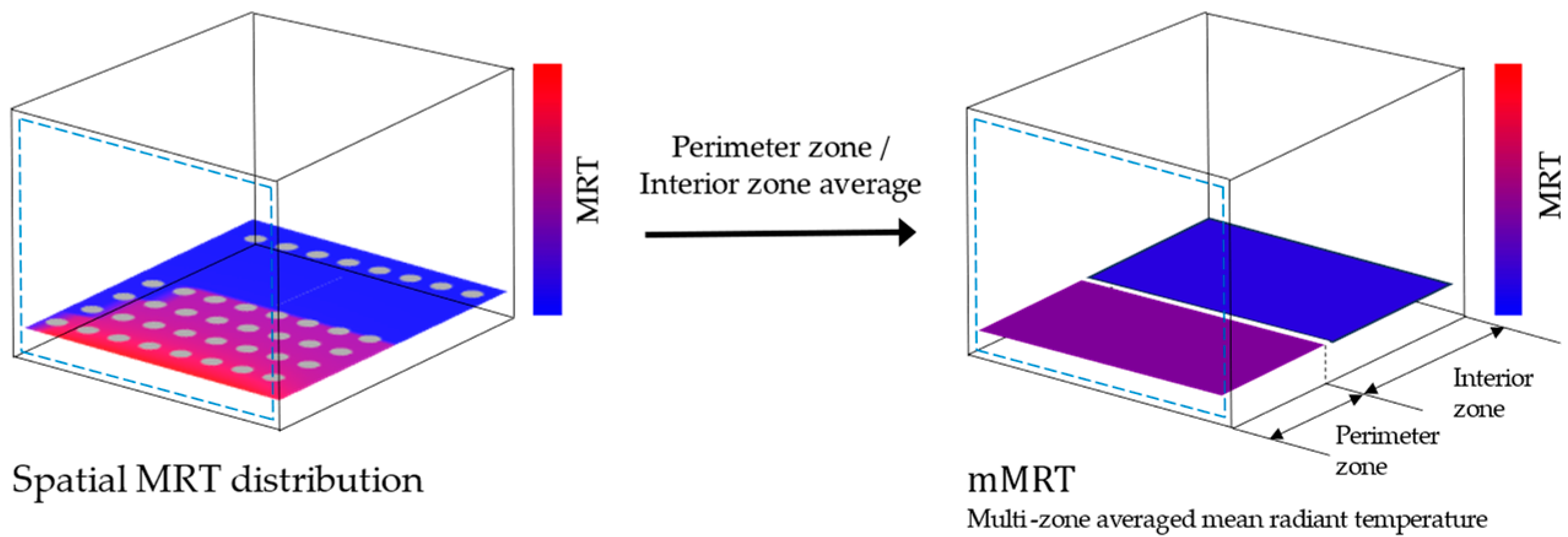
For large indoor spaces such as large offices, stadiums, or airports, the heating and cooling control is organized by dividing the space into distinct zones. The multi-zone averaged MRT (mMRT) method involves partitioning the indoor space into perimeter and interior zones, calculating the MRT for each zone, and then averaging these values to obtain a representative MRT. Figure 2 shows a schematic illustrating the process of calculating the mMRT. Equation (4) is used for calculating the mMRT in the perimeter zone, and Equation (5) is applicable for the interior zone.
m M R T P e r i . ( t ) = i P e r i . t ¯ r i , t n ( i P e r i . )
m M R T I n t . ( t ) = i I n t . t ¯ r i , t n ( i I n t . )
where t ¯ r is the MRT [°C], i is the MRT calculation point, t denotes time, and n represents the number of calculation points. This method manages the heating and cooling system by dividing the space into interior and perimeter zones, commonly used in large areas such as big offices. However, it is not suitable for controlling localized areas with devices such as radiators or small air conditioners.
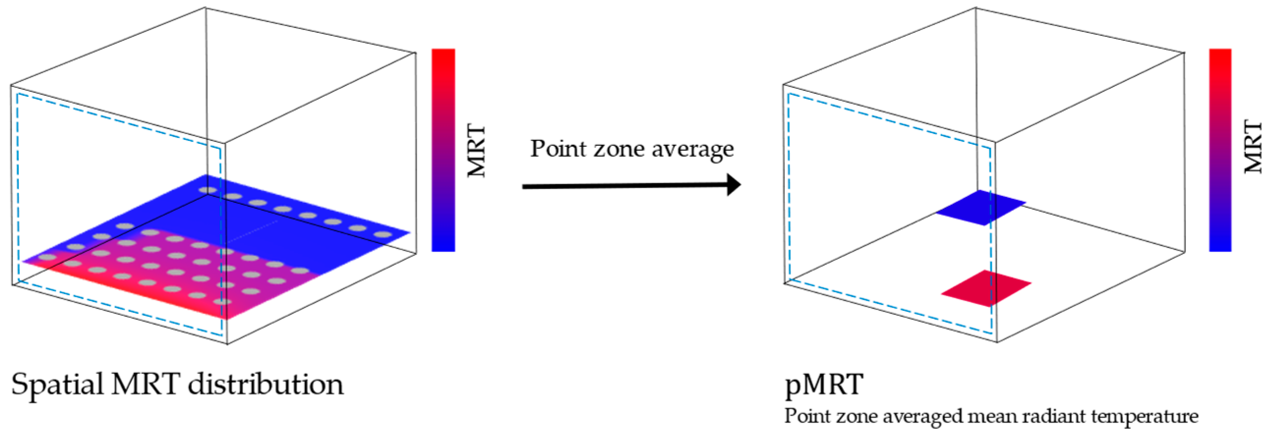
The sub-zonal method is used when individual control of localized spaces is necessary. Zampetti et al. [15] employed a sub-zonal method, where an IR scanning system was installed at the center of the target space to measure the thermal comfort in each sub-zone and independently control two electronic heaters based on the collected data. The point-zone MRT (pMRT) method involves the calculation of a representative value by averaging MRT measurements performed at specific points within a designated indoor zone. Figure 3 shows a schematic illustrating the process of calculating the pMRT. Equation (6) is formulated to derive the control target position exclusively.
p M R T i , t = t ¯ r i , t
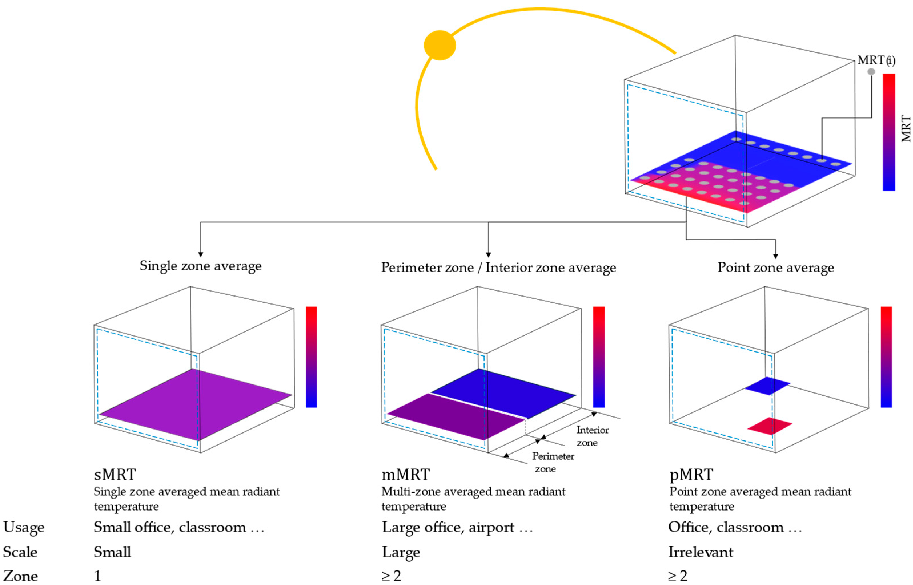
where t ¯ r is the MRT [°C], i is the MRT calculation point, and t denotes time. This method can be used when a radiator or small air conditioner is installed to control a specific sub-area. Figure 4 provides a brief overview of the schematics for the three representative value calculation methods: sMRT, mMRT, and pMRT.
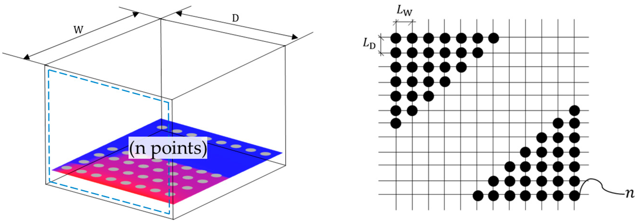
This study identified three calculation methods based on the building’s scale, usage, and applied conditions of equipment systems. Each of these methods can be applied when multi-point measurement is feasible. As the number of points increases, the calculation process becomes longer, which may be a drawback for real-time monitoring. Therefore, selecting an appropriate number of points is crucial, and this number may vary depending on the building’s scale and shape. The method for setting the spacing between points is as follows: one approach involves designing the number of points by evenly dividing the width and height of the target space, while another involves fixing the spacing between MRT calculation points and evenly distributing them. Figure 5 illustrates the design method for calculation points in space used for the MRT(i) calculation model. The figure on the left shows the distribution of points based on the width and height of the target space, and that on the right depicts the spacing of calculation points for the multi-point measurement method. Equations (7) and (8) describe the method for evenly dividing the width and height of the target space, respectively.
L W = W n 1
L D = D n 1
where L W is the width of the calculation points, L D is the depth of the calculation points, W is the width of the target space, D is the depth of the target space, and n is the number of calculation points. This method is suitable for spaces with a rectangular or square shape. However, if the space has a more irregular shape, the spacing of the calculation points should be fixed, and the width and height of the indoor area should be evenly divided for measurement. Equation (9) expresses a method for evenly dividing calculation points at fixed spacing.
L W = L D L m a x
where L m a x is the permissible spacing between calculation points along both horizontal and vertical directions. L m a x is selected considering the window width and the building scale. However, if the window is a standard type without any unique features, a spacing of 10 cm is selected.

4. Experiment and Result

4.1. Experiment Set-Up

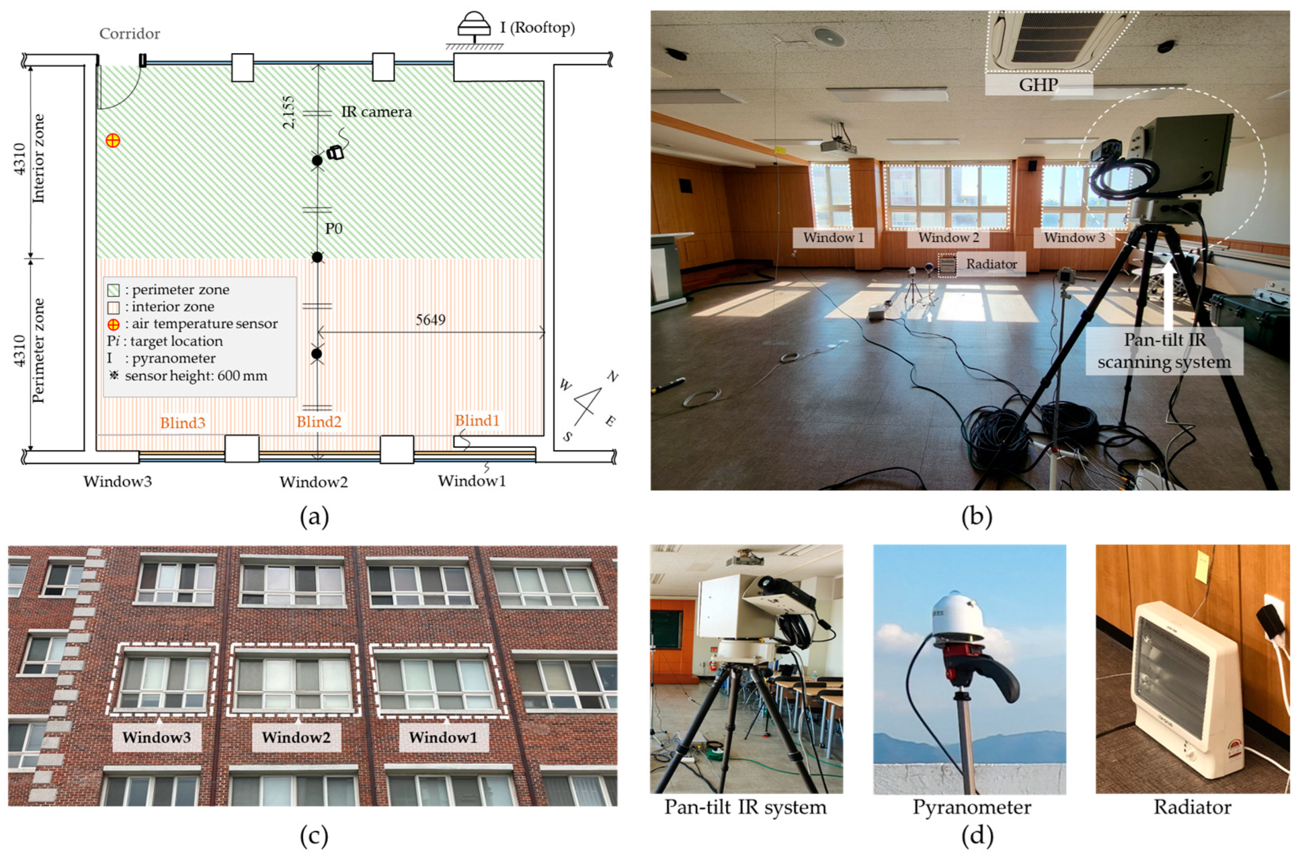
To determine the representative MRT value for the target space, a field experiment was conducted to compare MRT values obtained using the existing and proposed methods. Figure 6 shows the floor plan of the experimental space and installed equipment. The experiment was conducted within a university lecture room in Daegu, South Korea (latitude: 35.86, longitude: 128.49). The lecture room had internal dimensions of 8.6 m × 11.4 m × 2.9 m, with a glass wall on the north side and three windows with roller blinds installed on the south side. Three virtual sensors were modeled for the center of the room (P0), the perimeter zone (P1), and the interior zone (P2). The points for measuring the single-location MRT of the perimeter and interior zones were chosen as the center of each zone. In general, the depth of the perimeter zone is defined as twice the height from the floor to the ceiling [24]. In this study, the depth extending to the center of the zone was used to define the perimeter zone [5]. The sMRT was calculated based on the entire space, while the mMRT_(Peri.) and mMRT_(int.) were calculated for the perimeter and interior zones, respectively. The calculation of pMRT was not conducted in this experimental study.
To assess the differences and distribution characteristics of MRT based on measurement locations, a pan-tilt IR scanning system developed in a prior study [22] was utilized. The room was divided into 2500 equal sections to determine the measurement locations. An air temperature sensor was placed next to the gas heat pump (GHP) controller, ensuring that it was not influenced by solar radiation.
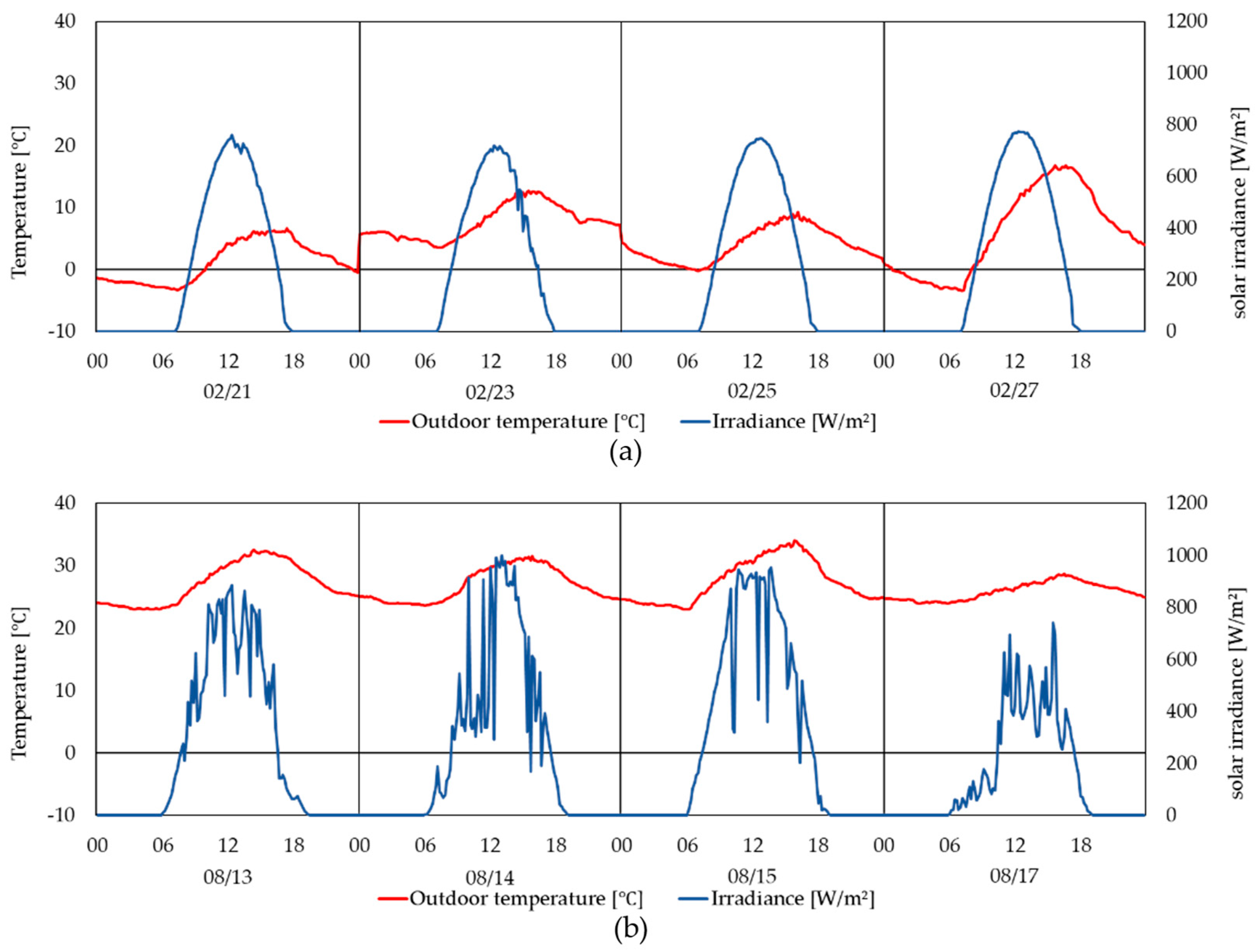
Table 2 presents cases categorized based on the control of the radiant heating and cooling systems on days with similar outdoor temperatures and solar irradiance during the heating and cooling seasons. The cases included natural conditions, a GHP, a roll blind which controls shortwave radiation or solar irradiance, and a radiator. The GHP system was set to a temperature of 24 °C and operated from 09:00 to 18:00. Figure 7 illustrates the graphs of outdoor temperature and irradiance for the heating (Figure 7a) and cooling (Figure 7b) seasons.
The findings of previous studies were employed to derive the MRT. Previous studies utilized factors such as unshaded fraction ( F u ), horizontal view factor (HVF), sky view factor (SVF), sunlit factor ( F s u n l i t ), angle factor ( F i j ), and solar transmittance ( T s o l ) in their results. The unshaded fraction ( F u ) indicates the percentage of the area above a window that remains unobstructed by elements such as awnings and is directly exposed to sunlight. This value is determined by considering the positions of the window, awning surfaces, and the sun [25]. The horizontal view factor (HVF) and sky view factor (SVF) only consider the spatial relationship between the window and awning surface [26]. The sunlit factor ( F s u n l i t ) indicates whether solar radiation reaches a specific location. It is calculated based on the positions of occupants, windows, awning surfaces, and the sun. The results are expressed as 0 (no solar radiation) or 1 (solar radiation present). It is calculated using three-dimensional (3D) model-based calculation tool, while considering the locations of the occupant and internal surfaces [26]. The angle factor ( F i j ) is determined using 3D model-based software, which calculates angle coefficients, and considers the positions of the occupant and internal surfaces [27]. For the calculation, the occupant was assumed to be seated with a height set to 600 mm. The solar transmittance ( T s o l ) refers to the ratio of solar energy that passes through the window, and it varies based on the glass’s physical properties. It is calculated using the WINDOW6 program and a curve fitting method to consider changes in the sun’s position [19]. The amount of solar radiation that enters the room is determined by this transmittance. The sunlit factor was assessed at three points (P0, P1, P2). Total solar radiation was determined using the decomposition model [28], where direct solar radiation and diffuse solar radiation were distinguished.
Table 3 presents the specifications of the equipment used for measurements. t ¯ r = t a was measured using a thermo-hygrometer. Single-location and area-weighted measurements were performed using a pan-tilt IR scanning system. The three MRT values estimated in this study were obtained using a pan-tilt IR scanning system and a pyranometer.

4.2. Result

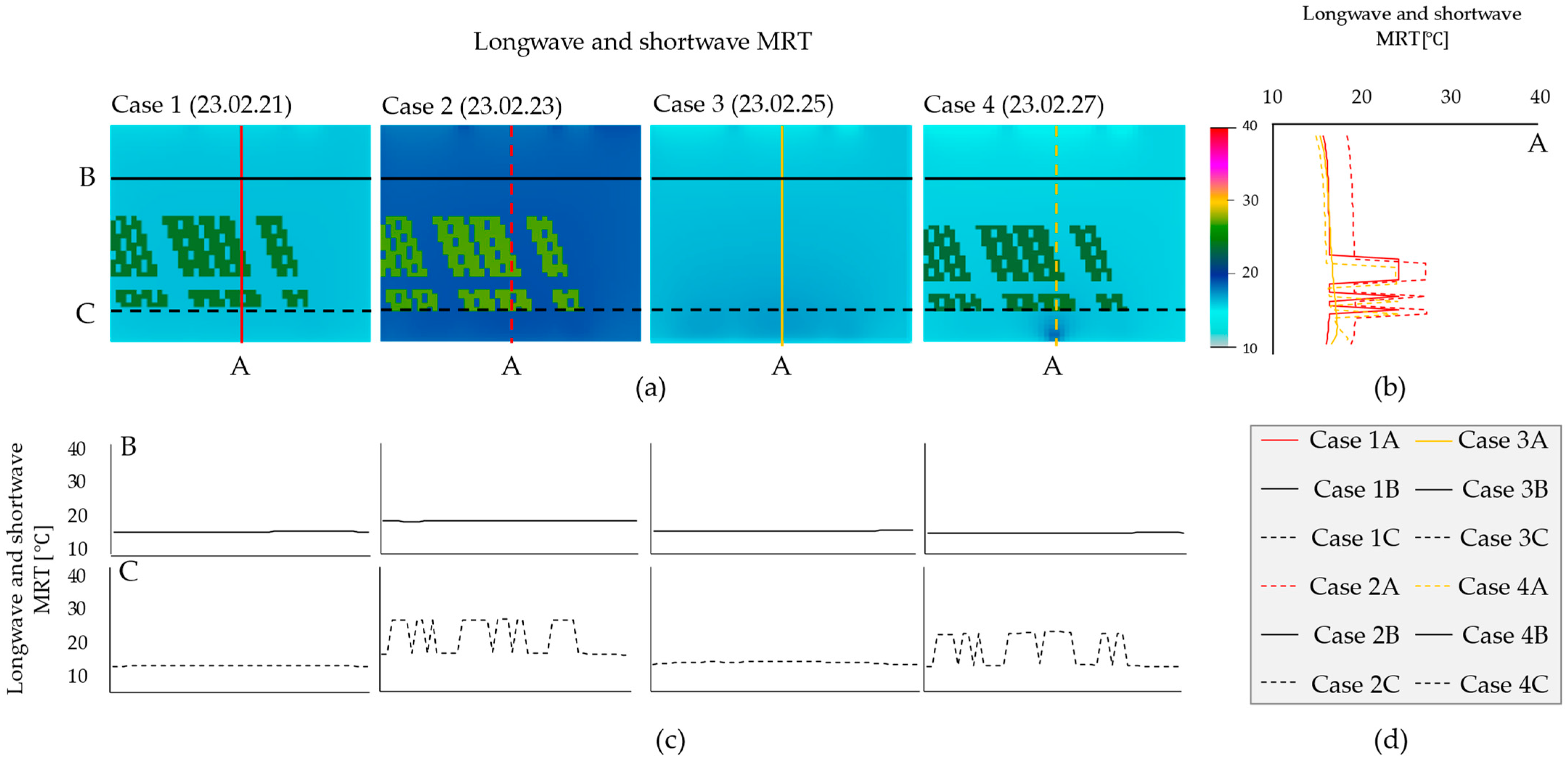
Figure 8 illustrates the MRT and its distribution across different cases during the heating season. Figure 8a shows an indoor heatmap of the MRT measurements, and Figure 8b shows the MRT for column A across various cases. Figure 8c shows the MRT for rows B and C, and Figure 8d presents the legend. In Case 3, rows B and C showed similar MRT distributions owing to the roll blinds managing solar radiation. In Case 2, controlling the air temperature with the GHP also affected the MRT. Specifically, in row A of Case 2, a noticeable difference of at least 3 °C was observed compared to the other cases. In Case 4, while controlling the radiator did not result in a significant difference from Case 1, certain changes were still evident in the heatmap.
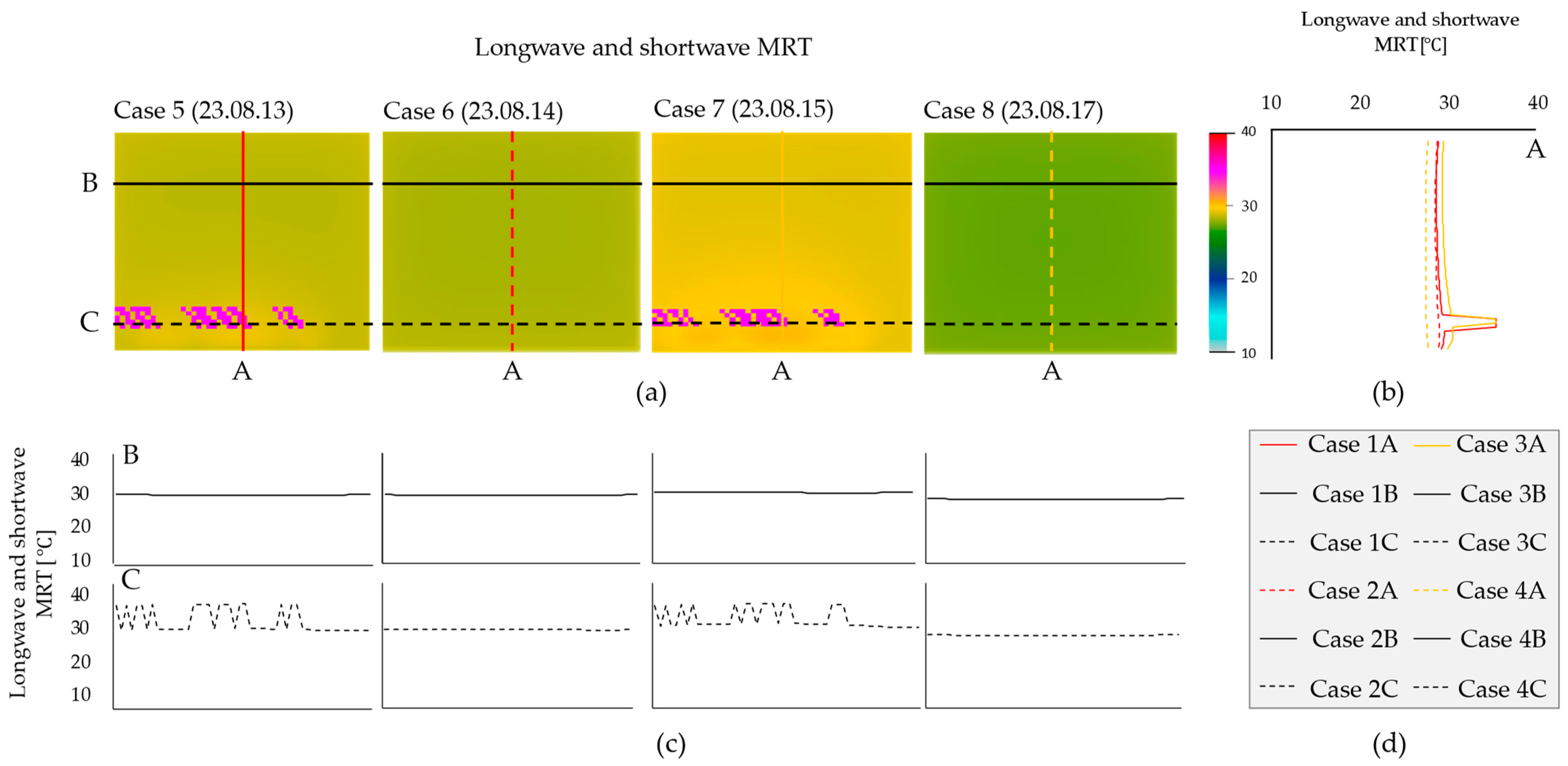
Figure 9 shows the MRT and its distribution for different cases during the cooling season. Cases 5 and 7 exhibited similar heatmaps, with a temperature difference of approximately 1 °C, except in areas influenced by solar radiation, as shown in column A. Row B also indicated differences of up to 1.2 °C, and row C exhibited a 1 °C difference at points excluding those affected by solar radiation. These variations were attributed to the impact of the GHP system controlling the air temperature. Comparing Case 6 and Case 8, it was observed that the heatmaps were similar owing to the roll blind control. The MRT difference between rows B and C was up to 1.3 °C, and column A showed a difference of approximately 1 °C. These variations were attributed to the impact of the GHP system controlling the air temperature. Figure 8 and Figure 9 illustrate the variations and distribution of MRT in response to the radiation and control of indoor equipment systems.
Table 4 presents a comparison of representative MRT values during the heating season, derived using the existing and proposed methods. The spatial MRT data were visually represented as a heatmap showing the spatial distribution of MRT values. The Min–Max values indicate the minimum and maximum MRT values distributed within the heatmap. A comparison of Cases 1 and 4 indicated an external air temperature average of approximately 4 °C higher, leading to a 1 °C increase in the overall temperature. For P2, the temperature difference remained within ±0.5 °C, whereas for P1, the difference was within ±0.5 °C, except at 09:05. In Case 4, under radiator control, the temperature did not show significant differences but was relatively slightly higher compared to other conditions. It was observed that the sMRT and t a measured at 09:05 in Case 1 differed by 2.2 °C each. Further, a 1 °C difference was observed with P0, and the area-weighted average also differed by 1.6 °C. In Case 2, the MRT values for P1 and the mMRT perimeter zone varied by 3.7–4.7 °C throughout the period. Similarly, the MRT values for P2 and the mMRT interior zone varied by 3.1–4.4 °C. These differences were attributed to the effects of solar radiation and the influence of the GHP controlling the air temperature. In Case 3, under the roll blind control (i.e., the awning is lowered), both the existing and proposed methods showed measurements within ±1 °C owing to the control of solar irradiance (shortwave radiation). Most of the P0 and area-weighted measurements in this case were within ±0.5 °C, and t ¯ r = t a at 09:05 was lower compared to other calculation methods, except in Case 3.
Table 5 presents a comparison of the representative MRT values during the cooling season derived by existing and proposed methods. During the cooling season, the MRT values did not show significant differences based on the measurement method, unlike in the heating season. At 12:05 in Cases 6–8, the sMRT values varied depending on the equipment system control. Although each system control resulted in a decrease in the sMRT, the most significant drop to 25.7 °C occurred when both the roll blind and GHP were controlled together. When only the GHP was controlled, the most noticeable difference between the air temperature and the sMRT was observed. The sMRT reduced to 26.7 °C under GHP control alone. Thus, although the air temperature remained relatively stable, the gap between the air temperature and the MRT widened. Therefore, relying solely on the air temperature data may not provide an accurate assessment of the thermal environment, as the sMRT also decreases when the air temperature is controlled. It is evident that controlling the GHP is more effective for controlling the MRT and the air temperature, compared to scenarios wherein only the roll blind or no control is applied without controlling the GHP. The MRT decreases progressively with equipment system control, with the most effective results achieved when both the roll blind and the GHP are controlled together. During the cooling season, the values for P1, P2, and pMRT showed insignificant variation, in contrast to that in the heating season. This limited variation was attributed to the specific virtual occupant locations used in the study. It is likely that changing these locations to areas with direct sunlight would reveal more noticeable differences.
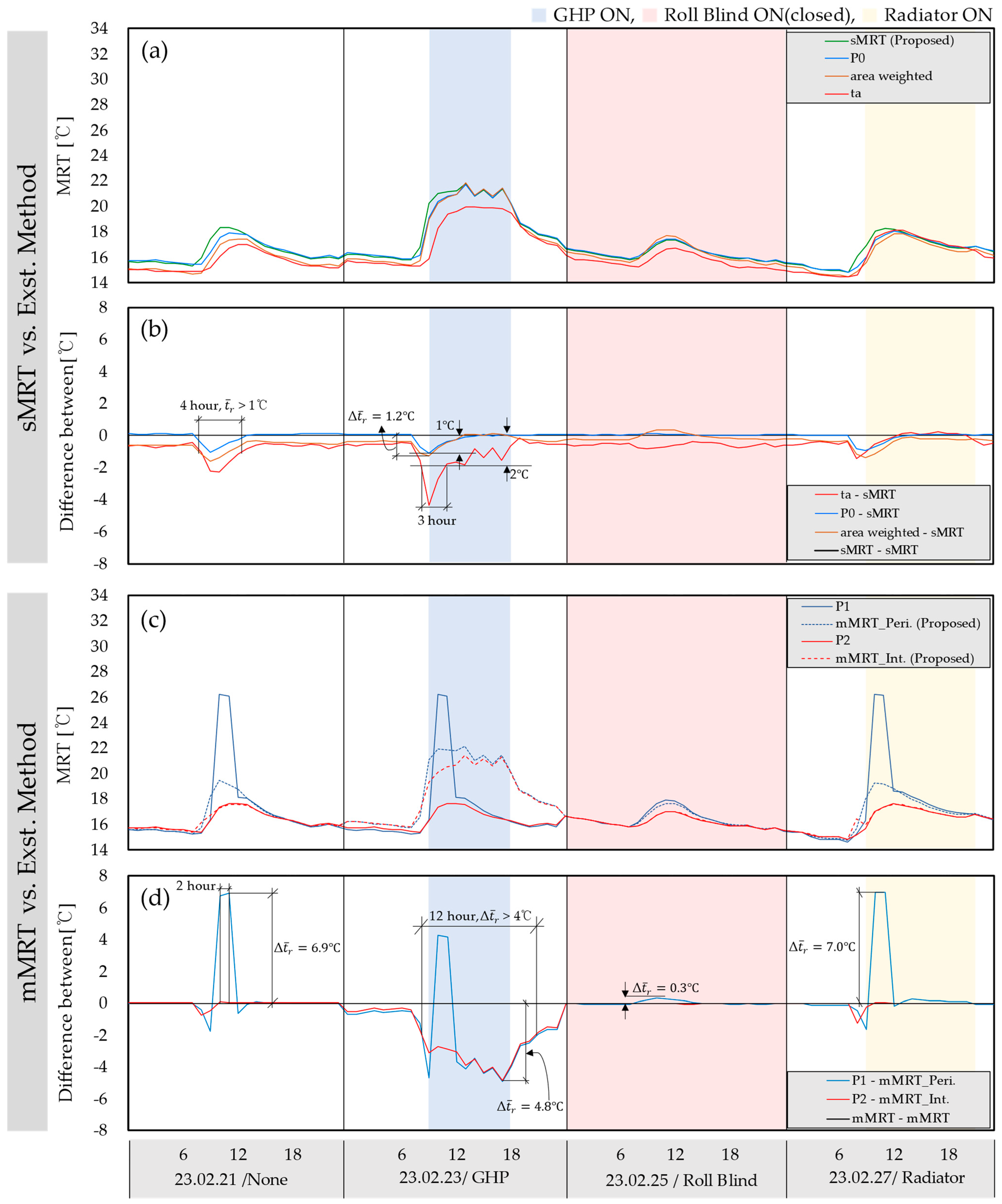
Figure 10 shows a comparison of representative values based on the method for deriving the MRT for the heating season. Figure 10a,c illustrate the representative value derivation methods for sMRT and mMRT, while Figure 10b,d show the errors between these methods. When “None” was applied, the time period during which the area-weighted method differed from the sMRT by more than 1 °C lasted for at least 4 h. Under the P0 condition, a difference greater than 0.5 °C persisted for approximately 4 h. For the method of using a representative value of the entire space, measurements at the center point can be more advantageous than using the area-weighted method. However, the situation varied under conditions of insolation. When the GHP was controlled, it was observed that the time during which t ¯ r = t a and the MRT differed by more than 1 °C lasted for over 7 h. Further, it was confirmed that the period with a difference of at least 2 °C lasted for approximately 3 h or more, with the maximum difference reaching up to 4 °C. As noted in previous reports, this study also confirmed that choosing a representative MRT value based on air temperature was not recommended. When comparing roll blind control, it was observed that the MRT was lower when the roll blind was in use, despite the outside temperature being higher at that time. Even under similar outside temperature conditions, it was confirmed that the radiant temperature increased owing to heat gain from the awning sunlight depending on the roll blind control. The impact of the radiator did not influence the overall MRT. A more noticeable difference was observed between the perimeter and the interior zones. For the “None” condition, P1 exhibited a difference of up to 6.9 °C compared to the mMRT, lasting for approximately 2 h. This was possibly attributable to solar gain. With GHP control, it was observed that the MRT difference for P1 of 4 °C or higher persisted for at least 12 h. P2 also showed a difference of up to 4.8 °C, which was attributed to the effect of the GHP on controlling the air temperature. With roll blind control, it was observed that the MRT difference was minimal, up to 0.3 °C. In contrast, with the radiator, the difference between P1 and the MRT reached up to 7 °C.
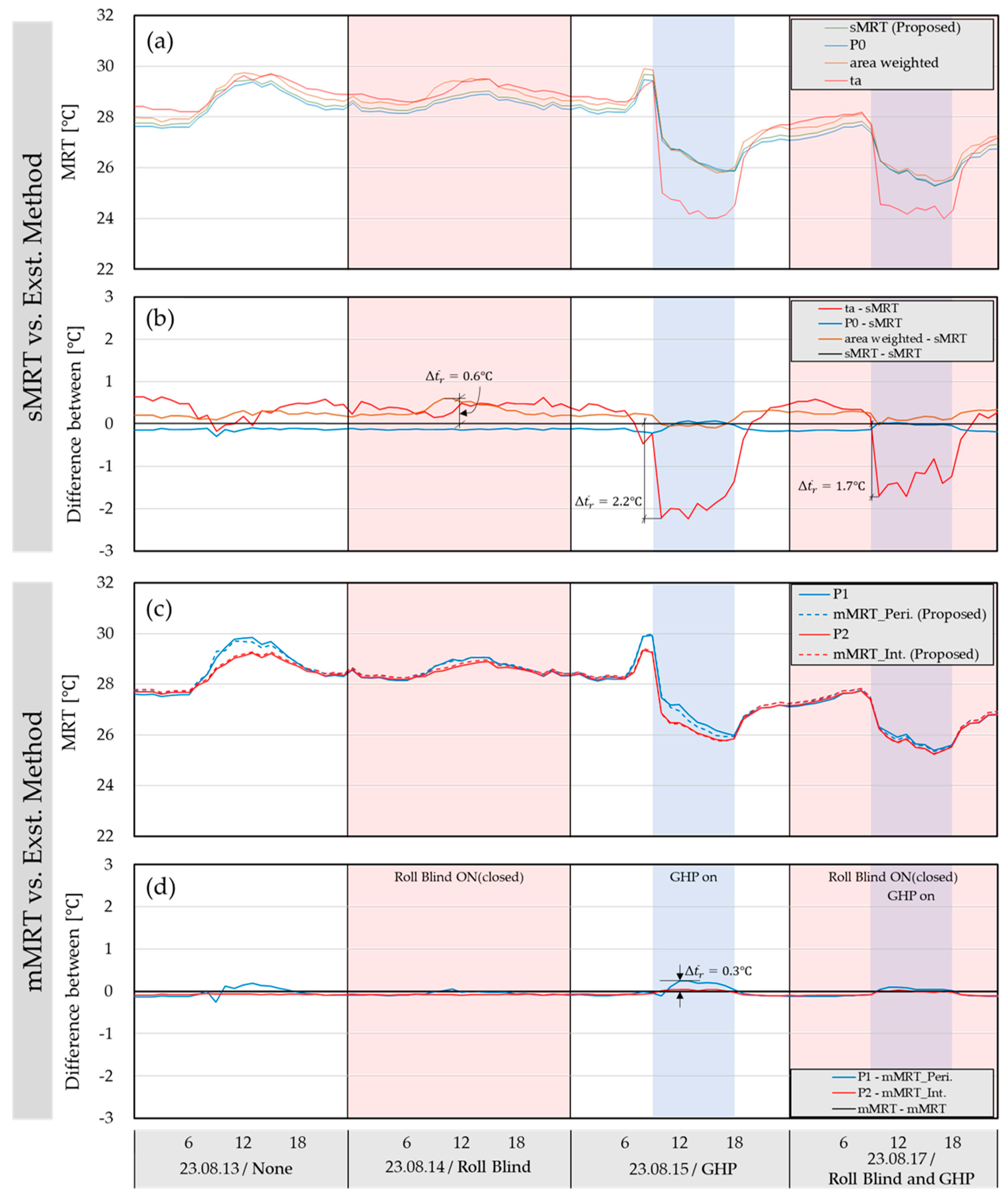
Figure 11 shows the comparison of representative values by method for deriving the MRT for the cooling season. Figure 11a,c illustrate the methods for deriving representative values of the sMRT and the mMRT, while Figure 11b,d display the errors between these methods. It was confirmed that there was almost no error in the P0 method for deriving the representative value of the sMRT. For the case where t ¯ r = t a , it was observed that the maximum difference was 0.6 °C with roll blind control. When GHP control was applied, it was confirmed that the difference exceeding 1 °C lasted for 8 h, with a maximum difference of 2.2 °C. When both the roll blind and the GHP were controlled together, an error of up to 1.7 °C was observed. In the case of the perimeter and interior zones, controlling the GHP resulted in a difference of up to 0.3 °C.
Figure 10 and Figure 11 confirm that the average radiation temperature was influenced by GHP control during both the heating and cooling seasons. Changes in wall surface temperature owing to convective heat transfer impacted the average radiation temperature. Specifically, it was observed that the MRT value significantly differed from the air temperature during the heating season. This highlights the importance of considering both air temperature and MRT when managing air conditioning.

5. Conclusions

To effectively control the thermal environment of occupants in indoor spaces through heating and cooling systems, it is crucial to monitor various physical environmental changes within the space. A recent study by M. Hawks et al. [29] reported that MRT measurement is significantly lacking in the industry, and this absence of MRT data limits the effectiveness of control systems. Research on MRT measurement [19,30] using computer simulation techniques has progressed to the point of enabling the analysis of spatial distributions of MRT values through experiments under various heating and cooling conditions. This progress has facilitated a visual analysis of the variations in MRT values depending on the occupants’ locations within a single space. However, to effectively apply the comprehensive measurement and evaluation results of the radiant environment in a space to the control of heating and cooling systems, a single representative MRT value is needed for the system’s feedback loop.
In this study, the existing MRT calculation methods were reviewed. Consequently, new methods for calculating representative MRT values were proposed. The proposed methods were classified into three approaches, considering factors such as building scale and use, equipment system type, and applied conditions. The proposed methods were based on the calculation of representative values as the average of the MRT, which were unevenly distributed, by dividing them into detailed areas (i.e., whole single zone, perimeter/interior zone, and sub-zone). Through experimental studies, the proposed method was tested under various operating conditions of equipment systems during both summer and winter. Experiments confirmed that the sMRT and the air temperature differed by up to 4 °C during the heating season. In the perimeter zone, the difference between the mMRT and the MRT under the measurement conditions of P1 reached up to 7 °C. During the cooling season, controlling the GHP resulted in a maximum difference of 2.2 °C. When both the roll blind and the GHP were controlled together, the maximum difference observed was 1.7 °C. It was confirmed that controlling the GHP altered the air temperature and increased the discrepancy with the MRT. This occurred because while the air temperature changed rapidly with GHP control, the mean radiant temperature changed minimally, leading to a significant deviation between the air temperature and the MRT. These findings indicate that relying solely on air temperature measurements to assess the indoor thermal environment has limitations, even in spaces with controlled air conditioning. The experimental results highlighted that considering only air temperature was insufficient for effectively managing various cooling and heating systems.
The purpose of this study was to examine the changes in MRT distribution and the differences in MRT values between the proposed and existing methods when shade, HVAC, and a radiator were in operation and under natural conditions. This study did not cover system control based on MRT and air temperature. In future research, the applicability of controlling heating and cooling systems based on operative temperature (OT) or predicted mean vote (PMV) will be investigated.
While assessing the thermal environment in buildings is crucial, current indoor thermal environment data from heating and cooling systems are limited to air temperature. To account for the comprehensive thermal environment, including the shape of a building, the type of heating and cooling equipment, and the impact of solar radiation owing to shading control, radiant environment information must be considered. Consequently, the integration of air temperature with mean radiant temperature is expected to offer new insights that have not previously been available to occupants and individual heating and cooling control systems.

Author Contributions

Writing—original draft preparation, methodology, data curation, visualization, S.-J.K.; Conceptualization, writing—review and editing, J.-H.J.; Conceptualization, writing—review and editing, methodology, supervision, D.-S.L.; All authors have read and agreed to the published version of the manuscript.

Funding

This research was funded by a National Research Foundation of Korea (NRF) grant (NRF-2022R1C1C2007250) funded by the government of the Republic of Korea (MSIP).

Data Availability Statement

The original contributions presented in the study are included in the article, further inquiries can be directed to the corresponding author.

Conflicts of Interest

The authors declare no conflicts of interest.

Nomenclature

Symbols
t ¯ r mean radiant temperature (°C)
t S j j-th indoor surface temperature (°C)
a j j-th indoor surface area ( m 2 )
T S j ( j ,t)absolute surface temperature of indoor surface j at time t
F i j angle factor
f p r o j projected area factor of human body surface
F s u n l i t sunlit factor
I D N direct normal irradiance (W/m2)
I d i f diffuse irradiance (W/m2)
α k shortwave radiation absorption coefficient ( α k = 0.57)
i MRT calculation point
ttime
n, n number of calculation points
P e r i . perimeter zone
I n t . interior zone
L W width of calculation points
L D depth of calculation points
W width of a target space
D depth of a target space
L m a x permissible spacing between calculation points along both horizontal and vertical directions
F u unshaded fraction
T s o l solar transmittance
Abbreviations and acronyms
MRTmean radiant temperature
PMVpredicted mean vote
GTglobe thermometer
CTcontact thermometer
IRinfrared
Win.winter
Sum.summer
S.L.single location
A.W.area weighted
S.Z.sub-zonal
sMRTsingle-zone averaged mean radiant temperature
mMRTmulti-zone averaged mean radiant temperature
pMRTpoint-zone mean radiant temperature
HVFhorizontal view factor
SVFsky view factor
GHPgas heat pump
Greek letters
ε emissivity
σ Stefan–Boltzmann constant ( σ = 5.67 · 10 8 W/m2K4)

References

  1. Park, J.; Kim, T.; Lee, C.-s. Development of Thermal Comfort-Based Controller and Potential Reduction of the Cooling Energy Consumption of a Residential Building in Kuwait. Energies 2019, 12, 3348. [Google Scholar] [CrossRef]
  2. Deng, Z.; Chen, Q. Artificial Neural Network Models Using Thermal Sensations and Occupants’ Behavior for Predicting Thermal Comfort. Energy Build. 2018, 174, 587–602. [Google Scholar] [CrossRef]
  3. Ku, K.L.; Liaw, J.S.; Tsai, M.Y.; Liu, T.S. Automatic Control System for Thermal Comfort Based on Predicted Mean Vote and Energy Saving. IEEE Trans. Autom. Sci. Eng. 2015, 12, 378–383. [Google Scholar] [CrossRef]
  4. Dogan, A.; Kayaci, N.; Demir, H.; Kemal, M. Energy & Buildings An Experimental Comparison of Radiant Wall and Ceiling Cooling System Integrated with Ground Source Heat Pump and Direct Expansion Fan Coil System in a Highly Glazed Office Room. Energy Build. 2023, 273, 112412. [Google Scholar] [CrossRef]
  5. Hwang, R.L.; Fang, P.L.; Chen, W.A. Impact of Solar Radiation on Indoor Thermal Comfort near Highly Glazed Façades in a Hot-Humid Subtropical Climate: An Experimental Evaluation. Build. Environ. 2023, 243, 110725. [Google Scholar] [CrossRef]
  6. Piasecki, M.; Fedorczak-cisak, M.; Furtak, M.; Biskupski, J. Experimental Confirmation of the Reliability of Fanger’ s Thermal Comfort Model—Case Study of a Near-Zero Energy Building (NZEB) O Ffi Ce Building. Sustainability 2019, 11, 2461. [Google Scholar] [CrossRef]
  7. Sung, S.H.; Yun, W.S.; Ryu, W.; Seo, H.; Hong, W.H. Development of Mean Radiant Temperature Virtual Sensor for Core and Perimeter Zones during the Summer Using Random Forest. J. Archit. Inst. Korea 2023, 39, 171–177. [Google Scholar] [CrossRef]
  8. Kubwimana, B.; Seyednezhad, M.; Najafi, H. Thermoelectric-Based Radiant Cooling Systems: An Experimental and Numerical Investigation of Thermal Comfort. Energies 2023, 16, 6981. [Google Scholar] [CrossRef]
  9. Huang, L.; John, Z. Critical Review and Quantitative Evaluation of Indoor Thermal Comfort Indices and Models Incorporating Solar Radiation Effects. Energy Build. 2020, 224, 110204. [Google Scholar] [CrossRef]
  10. Aparicio, P.; Salmerón, J.M.; Ruiz, Á.; Sánchez, F.J.; Brotas, L. The Globe Thermometer in Comfort and Environmental Studies in Buildings. Rev. Constr. 2016, 15, 57–66. [Google Scholar] [CrossRef]
  11. Uribe, D.; Vera, S. Assessment of the Effect of Phase Change Material (PCM) Glazing on the Energy Consumption and Indoor Comfort of an Office in a Semiarid Climate. Appl. Sci. 2021, 11, 9597. [Google Scholar] [CrossRef]
  12. Wang, D.; Chen, G.; Song, C.; Liu, Y.; He, W.; Zeng, T.; Liu, J. Experimental Study on Coupling Effect of Indoor Air Temperature and Radiant Temperature on Human Thermal Comfort in Non-Uniform Thermal Environment. Build. Environ. 2019, 165, 106387. [Google Scholar] [CrossRef]
  13. Chang, H.; Park, S.-H.; Park, B. Analysis on Indoor Thermal Comfort of Buildings in Campus during Intermediate Season. J. Arch. Inst. Korea 2014, 16, 187–194. [Google Scholar]
  14. Arnesano, M.; Calvaresi, A.; Pietroni, F.; Zampetti, L.; Magnani, S.; Casadei, O.; Revel, G.M. A Sub-Zonal PMV-Based HVAC and Façade Control System for Curtain Wall Buildings. Proceedings 2018, 2, 1596. [Google Scholar] [CrossRef]
  15. Zampetti, L.; Arnesano, M.; Revel, G.M. Experimental Testing of a System for the Energy-Efficient Sub-Zonal Heating Management in Indoor Environments Based on PMV. Energy Build. 2018, 166, 229–238. [Google Scholar] [CrossRef]
  16. Park, J.; Choi, H.; Kim, D.; Kim, T. Development of Novel PMV-Based HVAC Control Strategies Using a Mean Radiant Temperature Prediction Model by Machine Learning in Kuwaiti Climate. Build. Environ. 2021, 206, 108357. [Google Scholar] [CrossRef]
  17. Chaudhuri, T.; Soh, Y.C.; Bose, S.; Xie, L.; Li, H. On Assuming Mean Radiant Temperature Equal to Air Temperature during PMV-Based Thermal Comfort Study in Air-Conditioned Buildings. In Proceedings of the IECON 2016-42nd Annual Conference of the IEEE Industrial Electronics Society, Florence, Italy, 23–26 October 2016; pp. 7065–7070. [Google Scholar] [CrossRef]
  18. Guo, H.; Teitelbaum, E.; Houchois, N.; Bozlar, M.; Meggers, F. Revisiting the Use of Globe Thermometers to Estimate Radiant Temperature in Studies of Heating and Ventilation. Energy Build. 2018, 180, 83–94. [Google Scholar] [CrossRef]
  19. Lee, D.; Jo, J. Application of IR Camera and Pyranometer for Estimation of Longwave and Shortwave Mean Radiant Temperatures at Multiple Locations. Build. Environ. 2022, 207, 108423. [Google Scholar] [CrossRef]
  20. Kosiński, P.; Skotnicka-Siepsiak, A. Possibilities of Adapting the University Lecture Room to the Green University Standard in Terms of Thermal Comfort and Ventilation Accuracy. Energies 2022, 15, 3735. [Google Scholar] [CrossRef]
  21. Sung Jin, K.; Dong Seok, L. Method for Determining the Representative Mean Radiant Temperature for Heating and Cooling Control Application. J. Korean Inst. Archit. Sustain. Environ. Build. Syst. 2024, 18, 165–174. [Google Scholar]
  22. Lee, D.S.; Jo, J.H. Pan–Tilt Ir Scanning Method for the Remote Measurement of Mean Radiant Temperatures at Multi-Location in Buildings. Remote Sens. 2021, 13, 2158. [Google Scholar] [CrossRef]
  23. La Gennusa, M.; Nucara, A.; Rizzo, G.; Scaccianoce, G. The Calculation of the Mean Radiant Temperature of a Subject Exposed to the Solar Radiation—A Generalised Algorithm. Build. Environ. 2005, 40, 367–375. [Google Scholar] [CrossRef]
  24. Baker, N.; Steemers, K. Energy and Environment in Architecture a Technical Design Guide; Taylor & Francis: Abingdon, UK, 1998; p. 224. [Google Scholar]
  25. Choi, S.; Lee, D.; Jo, J. Method of Deriving Shaded Fraction According to Shading Movements of Kinetic Façade. Sustainability 2017, 9, 1449. [Google Scholar] [CrossRef]
  26. Lee, D.; Jo, J. Application of Simple Sky and Building Models for the Evaluation of Solar Irradiance Distribution at Indoor Locations in Buildings. Build. Environ. 2021, 197, 107840. [Google Scholar] [CrossRef]
  27. Lee, D.S.; Kim, E.J.; Cho, Y.H.; Kang, J.W.; Jo, J.H. A Field Study on Application of Infrared Thermography for Estimating Mean Radiant Temperatures in Large Stadiums. Energy Build. 2019, 202, 109360. [Google Scholar] [CrossRef]
  28. Kyung-soo, L.S.L. A Research on the Decomposition Model and Transposition Model Using the Measured Pyranometer Irradiation Data. J. Korean Sol. Energy Soc. 2018, 38, 1–20. [Google Scholar]
  29. Hawks, M.A.; Cho, S. Review and Analysis of Current Solutions and Trends for Zero Energy Building (ZEB) Thermal Systems. Renew. Sustain. Energy Rev. 2024, 189, 114028. [Google Scholar] [CrossRef]
  30. Guo, H.; Ferrara, M.; Coleman, J.; Loyola, M.; Meggers, F. Simulation and Measurement of Air Temperatures and Mean Radiant Temperatures in a Radiantly Heated Indoor Space. Energy 2020, 193, 116369. [Google Scholar] [CrossRef]
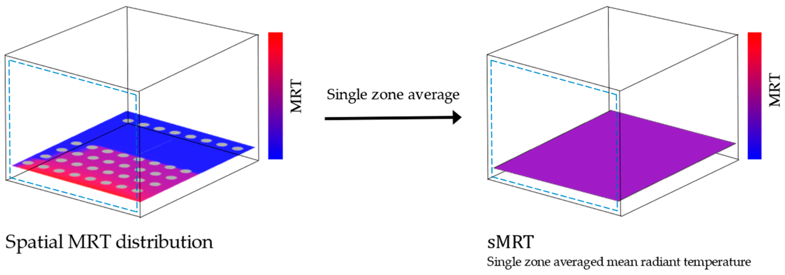
Figure 1. Schematic diagram for calculating sMRT.
Energies 17 05221 g001
Figure 2. Schematic diagram for calculating mMRT.
Energies 17 05221 g002
Figure 3. Schematic diagram for calculating pMRT.
Energies 17 05221 g003
Figure 4. Methods of deriving the three derivation representative MRT values.
Energies 17 05221 g004
Figure 5. Schematic diagram of MRT calculation points based on width and depth.
Energies 17 05221 g005
Figure 6. Experiment set-up. (a) floor plan; (b) arrangement of equipment for measuring indoor MRT; (c) external view of the target space; and (d) equipment for measuring MRT.
Energies 17 05221 g006
Figure 7. Outdoor temperature and solar irradiance. (a) heating season (Cases 1–4); and (b) cooling season (Cases 5–8).
Energies 17 05221 g007
Figure 8. Measurement results of MRT distributions during the heating season (09:05). (a) MRT distribution heatmap; (b) MRT heatmap A; (c) MRT heatmap B and C; and (d) legend.
Energies 17 05221 g008
Figure 9. Measurement results of MRT distributions during cooling season (09:05). (a) MRT distribution heatmap; (b) MRT heatmap A; (c) MRT heatmap B and C; and (d) legend.
Energies 17 05221 g009
Figure 10. Comparison of representative values by method for deriving MRT for the heating season. (a,c) methods for deriving representative values for sMRT and mMRT; (b,d) difference between methods for deriving representative values for sMRT and mMRT.
Energies 17 05221 g010
Figure 11. Comparison of representative values by method for deriving MRT for the cooling season. (a,c) methods for deriving representative values for sMRT and mMRT; (b,d) difference between methods for deriving representative values for sMRT and mMRT.
Energies 17 05221 g011
Table 1. Representative MRT derivation methods and instruments in existing studies.
YearBldg. TypeSeasonInstrumentRepresentative MRT *RadiantRef.
AirGTIRCT t ¯ r = t a S.L. A.W.S.Z.LWSW
2018OfficeWin. and sum.x x [1]
2019ChamberSum.x x [2]
2015OfficeSum.x x [3]
2023OfficeSum. x x xx[4]
2023ChamberSum. x x xx[5]
2019OfficeWin. x x xx[6]
2023ClassroomSum. x x xx[7]
2023ChamberNot presented x x xx[8]
2020OfficeWin. x x xx[9]
2016ChamberSum. x x xx[10]
2021OfficeSum. x x xx[11]
2019ChamberSum. x x x [12]
2014OfficeWin. x x x [13]
2020OfficeSum. x xx [14]
2018OfficeWin. x xx [15]
Abbreviation: Win. (winter), Sum. (summer), GT (globe thermometer), IR (infrared camera), CT (contact thermometer). * Representative MRT. t ¯ r = t a : method assuming that MRT is equal to air temperature. S.L.: single-location method selecting a single point at the center, perimeter, or interior zone. A.W.: area-weighted method averaging the indoor surface temperatures weighted by the area of each surface. S.Z.: sub-zonal method selecting various sub-zones (or point zones) and measuring separately.
Table 2. Control targets by case.
SeasonCasesSystem Type
HeatingCase 1None
Case 2GHP
Case 3Roll Blind
Case 4Radiator
CoolingCase 5None
Case 6Roll Blind
Case 7GHP
Case 8Roll Blind and GHP
Table 3. Specifications of the measuring devices.
Device NameSpecifications
Pan-tilt IR scanning system
(developed by Lee et al., 2021 [22])
ModelFLIR A310/±2 °C
Temperature range−20 to 350 °C
Accuracy±2%
IR resolution320 × 240 pixels
PyranometerModelMS-40
Irradiance range0 to 2000 W/m2
Accuracy±12 W/m2
Sensitivity7–14 µV/W/m2
Thermo-hygrometerModelTesto 174H
Operating temperature−20 to 70 °C
Accuracy(T) ± 0.5 °C
Resolution0.1 °C
Table 4. Comparison of representative MRT values during heating season, derived by existing and proposed methods.
Cases
System Type
Applied Methods *Measured Representative MRT Values
09:0512:0515:0518:05
Case 1
None
Measured dataSpatial
MRT data
Energies 17 05221 i001Energies 17 05221 i002Energies 17 05221 i003Energies 17 05221 i004
Min–Max15.7–24.216.6–26.716.1–17.115.7–16.4
Exst. t ¯ r = t a 15.217.016.415.6
Single locationP016.417.917.016.4
P1/P216.4/16.318.1/17.617.1/16.816.3/16.3
Area-weighted15.817.516.515.8
Prop. s M R T 17.418.116.916.3
m M R T Peri./Int.18.2/16.718.7/17.517.0/16.816.3/16.3
Case 2
GHP
Measured dataSpatial
MRT data
Energies 17 05221 i005Energies 17 05221 i006Energies 17 05221 i007Energies 17 05221 i008
Min–Max18.2–27.319.8–28.720.3–21.819.4–20.7
Exst. t ¯ r = t a 15.919.619.919.5
Single locationP019.121.021.420.2
P1/P216.4/16.318.1/17.617.1/16.816.3/16.3
Area-weighted19.021.021.320.1
Prop. s M R T 20.221.221.320.2
m M R T Peri./Int.21.1/19.421.8/20.721.4/21.220.1/20.1
Case 3
Roll Blind
Measured dataSpatial
MRT data
Energies 17 05221 i009Energies 17 05221 i010Energies 17 05221 i011Energies 17 05221 i012
Min–Max15.2–17.316.2–18.215.7–16.715.4–16.1
Exst. t ¯ r = t a 15.616.716.015.3
Single locationP016.617.416.516.0
P1/P217.0/16.217.9/17.016.6/16.316.0/15.9
Area-weighted16.617.716.415.8
Prop. s M R T 16.417.316.516.0
m M R T Peri./Int.16.7/16.217.6/17.016.6/16.416.0/15.9
Case 4
Radiator
(900 W)
Measured dataSpatial
MRT data
Energies 17 05221 i013Energies 17 05221 i014Energies 17 05221 i015Energies 17 05221 i016
Min–Max14.8–24.316.5–27.516.4–20.216.0–19.3
Exst. t ¯ r = t a 15.918.117.516.9
Single locationP016.018.017.516.9
P1/P216.3/15.718.7/17.617.9/17.217.0/16.7
Area-weighted15.617.817.316.6
Prop. s M R T 17.018.217.516.8
m M R T Peri./Int.18.0/15.918.8/17.617.7/17.316.9/16.7
* t ¯ r = t a : method assuming MRT is equal to air temperature. single location: method selecting a single point at the center, perimeter zone, or interior zone of the room for measurement. P0 is the center of room, P1 is the center of the perimeter zone, and P2 is the center of the interior zone. Area-weighted: method of averaging the indoor surface temperature weighted by the area of each surface. sMRT: method of averaging MRT by dividing the indoor space into n points. mMRT: method of averaging MRT by distinguishing between the perimeter and interior zone. Abbreviation: Exst. (Existing), Prop. (Proposed).
Table 5. Comparison of representative MRT values during cooling season, derived by existing and proposed methods.
Cases
System Type
Applied Methods *Measured Representative MRT Values
09:0512:0515:0518:05
Case 5
None
Measured dataSpatial
MRT data
Energies 17 05221 i017Energies 17 05221 i018Energies 17 05221 i019Energies 17 05221 i020
Min–Max28.6–35.429.1–33.929.2–30.128.7–29.1
Exst. t ¯ r = t a 28.829.629.729.3
Single locationP028.729.329.328.7
P1/P229.0/28.629.8/29.129.7/29.228.8/28.7
Area-weighted29.129.729.729.1
Prop. s M R T 29.029.429.428.8
m M R T Peri./Int.29.3/28.729.7/29.229.6/29.328.8/28.8
Case 6
Roll Blind
Measured dataSpatial
MRT data
Energies 17 05221 i021Energies 17 05221 i022Energies 17 05221 i023Energies 17 05221 i024
Min–Max28.5–29.028.7–29.228.9–29.328.6–29.0
Exst. t ¯ r = t a 28.829.429.529.2
Single locationP028.528.728.928.6
P1/P228.7/28.528.9/28.729.1/28.928.7/28.6
Area-weighted29.129.429.529.0
Prop. s M R T 28.628.929.028.7
m M R T Peri./Int.28.7/28.628.9/28.829.1/29.028.7/28.7
Case 7
GHP
Measured dataSpatial
MRT data
Energies 17 05221 i025Energies 17 05221 i026Energies 17 05221 i027Energies 17 05221 i028
Min–Max29.2–35.326.1–31.825.7–26.625.8–26.1
Exst. t ¯ r = t a 29.424.724.024.5
Single locationP029.426.726.125.9
P1/P229.9/29.327.2/26.526.4/26.026.0/25.8
Area-weighted29.926.726.026.0
Prop. s M R T 29.626.726.125.9
m M R T Peri./Int.30.0/29.326.9/26.426.2/25.925.9/25.9
Case 8
Roll Blind
and GHP
Measured dataSpatial
MRT data
Energies 17 05221 i029Energies 17 05221 i030Energies 17 05221 i031Energies 17 05221 i032
Min–Max27.4–27.825.6–26.025.4–25.825.5–25.7
Exst. t ¯ r = t a 27.724.424.324.3
Single locationP027.425.825.525.5
P1/P227.4/27.425.9/25.725.6/25.525.6/25.5
Area-weighted27.725.825.725.7
Prop. s M R T 27.525.725.525.6
m M R T Peri./Int.27.5/27.525.8/25.725.6/25.625.6/25.5
* t ¯ r = t a : method assuming MRT is equal to air temperature. single location: method selecting a single point at the center, perimeter zone, or interior zone of the room for measurement. P0 is the center of room, P1 is the center of the perimeter zone, and P2 is the center of the interior zone. Area-weighted: method of averaging the indoor surface temperature weighted by the area of each surface. sMRT: method of averaging MRT by dividing the indoor space into n points. mMRT: method of averaging MRT by distinguishing between the perimeter and interior zone. Abbreviation: Exst. (Existing), Prop. (Proposed).
Disclaimer/Publisher’s Note: The statements, opinions and data contained in all publications are solely those of the individual author(s) and contributor(s) and not of MDPI and/or the editor(s). MDPI and/or the editor(s) disclaim responsibility for any injury to people or property resulting from any ideas, methods, instructions or products referred to in the content.