Article

Machine Learning-Aided Dual-Function Microfluidic SIW Sensor Antenna for Frost and Wildfire Detection Applications

by
Amjaad T. Altakhaineh
1,
Rula Alrawashdeh
1,* and
Jiafeng Zhou
2,*
1
Electrical Engineering Department, Mutah University, Al-Karak 61710, Jordan
2
Department of Electrical Engineering and Electronics, University of Liverpool, Liverpool L69 3GJ, UK
*
Authors to whom correspondence should be addressed.
Energies 2024, 17(20), 5208; https://doi.org/10.3390/en17205208
Submission received: 5 September 2024 / Revised: 26 September 2024 / Accepted: 9 October 2024 / Published: 19 October 2024
(This article belongs to the Section F: Electrical Engineering)

Abstract

:
In this paper, which represents a fundamental step in ongoing research, a new smart low-energy dual-function half-mode substrate integrated waveguide cavity-interdigital capacitor (HMSIWC-DIC) antenna-based sensor is developed and investigated for remote frost and wildfire detection applications at 5.7 GHz. The proposed methodology exploits the HMSIW antenna-based sensor, a microfluidic channel (microliter water channel (50 μL)), interdigital capacitor technologies, and the resonance frequency parameters combined with machine learning algorithms. This allows for superior interaction between the water channel and the TE101 mode, resulting in high sensitivity (∆f/∆ε = 5.5 MHz/ε (F/m) and ∆f/∆°C = 1.83 MHz/°C) within the sensing range. Additionally, it exhibits high decision-making ability and immunity to interference, demonstrating a best-in-class sensory response to weather temperature across two ranges: positive (≥0 °C, including frost and wildfire) and negative (<0 °C, including ice accumulation). To address the challenges posed by the non-linear, unpredictable behavior of resonance frequency results, even when dealing with weak sensor antenna responses, an innovative sensory intelligent system was proposed. This system utilizes resonance frequency results as features to classify and predict weather temperature ranges into three environmental states: Early Frost, Normal, and Early Wildfire, achieving an accuracy of 96.4%. Several machine learning techniques are employed, including artificial neural networks (ANNs), random forests (RF), decision trees (DT), support vector machines (SVMs), and Gaussian processes (GPs). This sensor serves as an ideal solution for energy management through its utilization in RF-based weather temperature sensing applications. It boasts stable performance, minimal energy consumption, and real-time sensitivity, eliminating the necessity for manual data recording.

1. Introduction

Remotely monitoring the environmental temperature is of great importance for smart cities [1], as well as for industrial and environmental sensing [2] applications. For example, in renewable wind power farms, ice formation on wind turbines can reduce their power output by up to 30% per year [3]. In addition, around 1.7 billion people have been hit by natural disasters over the past decade, leaving behind more than 400,000 fatalities [4]. Apart from the well-known natural disasters such as earthquakes and flash floods, frost and wildfire disasters have destroyed agricultural crops and caused human losses, which can significantly degrade national economies and severely impact the global climate. For example, farmers in the Jordan Valley are affected by frost damage and their crops are destroyed yearly, resulting in financial losses exceeding tens of millions of USD. Recently, in August 2020 [5], flames ravaged several hectares of a date oasis at a time coinciding with the harvest season in Morocco. Furthermore, the losses resulting from wildfire disasters are not limited to damaged property; wildfires can reduce the effectiveness of solar power due to smoke and particulate matter blocking sunlight. Additionally, wildfires can damage wind farms and other renewable energy installations [6]. Unfortunately, such natural disasters occur suddenly, which makes early warning a very efficient way to mitigate the impact of these events. Therefore, designing early warning systems is essential to predicting or detecting early the presence of frost and wildfire disasters.
In fact, monitoring the medium’s temperature is one of the most effective forecasting methods and helps to detect the occurrence of frost disasters and forest fires early. National Weather Service forecasters consistently help farmers and firefighters by producing fire and frost weather forecasts on a daily basis during the warm and cold seasons [7]. To this end, several methods based on traditional temperature sensors (thermometers) have been used to detect and forecast the environmental temperature. Nonetheless, such sensors frequently demand specific requirements, such as installation and implementation, dedicated expert settings, and high-energy efficiency, which are factors that can consume considerable time and become unfeasible for the context of real-time monitoring in harsh environments [8]. Early Warning Systems (EWSs) are one of the major applications for wireless sensor networks (WSNs), in which the sensor nodes are designed to collaborate with the RF communication network to detect and transmit the sensing results [9,10,11]. Actually, the warning issued from the EWS should be reliable enough to prevent any wastage of resources spent in the reaction taken in response to the warning. However, WSN-based EWSs face several challenges that can degrade detection performance, such as real-time monitoring efficiency, the need to be provided with energy by a power supply, and the requirement of a transmission line connection between the sensor and the signal-processing system. On the other hand, energy consumption is a main concern in WSNs due to the limited energy resources equipped at the sensor nodes, as well as the difficulty faced when recharging or replacing batteries in areas that are usually widely spaced. Furthermore, these systems are compelled to activate a power-saving mode to conserve energy and resources, rendering them unsuitable for applications that require continuous, uninterrupted monitoring.
Over the last decade, sensors operating at RF frequencies have received huge applied research attention, since the technology can represent promising solutions for various fields and applications [12,13,14,15,16,17,18,19,20,21,22,23,24,25,26,27,28,29,30,31,32]. Such sensors offer a small footprint, non-intrusive detection, real-time monitoring, high detection capabilities, and high sensitivity. This results in the ability to integrate and implement them practically across wide areas, which have led to their widespread adoption in real Internet of Things (IoT) systems. Furthermore, RF-based sensors have the ability to be integrated into a wide range of areas without the need for any external electronic systems or transmission lines. This approach allows for simultaneous detection and signal processing within the sensor itself. As a result, it reduces the overall energy demand and supply requirements, enhancing efficiency and minimizing the need for additional power sources. This self-sufficiency makes RF-based sensors highly adaptable and energy-efficient for various applications that necessitate uninterrupted monitoring, even in environments where continuous operation without a saving mode is essential.
RF-based sensing follows a precise sensing process that allows for monitoring the interaction between the electric fields and the material under test, resulting in the observation of changes in the material’s properties (e.g., permittivity ε) in real time. This process can determine the properties of the tested samples by measuring the electromagnetic wave (EM) parameters. Furthermore, the RF-based sensors can be designed as radiators to act as a sensing platform while simultaneously transmitting the sensed signals. These structures, known as antenna sensors, have been adopted and developed for wireless ice accretion sensing [17], as well as material temperature monitoring [14,15,16,17,18,19,20,21,22,23,24,25], and crack propagation tracking [19]. Sensors based on RF antennas have attracted widespread attention because they are label-free, noninvasive, portable, affordable, environmentally friendly, sustainable, have low power consumption, and can integrate with the other parts of any sensor system. Regarding the antenna-based sensing methodology, antennas use various methods to measure and monitor the EM wave properties—these methods can be classified as resonate (standing wave) [17,31] and non-resonate (traveling wave) [32]. However, antennas operating based on resonance methods have become more popular since they can provide high reliability, accuracy, and sensitivity in detection. In addition, resonate antennas can offer multi-sensing parameters (parameters under test (PUT)) to measure the properties of the material under test (MUT) using both power and frequency measurements, such as resonance frequency, S-parameters, gain, efficiency, etc. In general, the performance of the sensor antenna primarily depends on the sensing area, as this area enhances the interaction between the material under test (MUT) and the antenna, leading to high sensitivity. However, based on the resonant method, achieving a robust sensing antenna is determined by providing a large distribution of capacitive elements. By doing so, the stored energy increases within the antenna, thereby enhancing its penetrating performance [12,13,14,15,16,17,18,19,20,21,22,23,24,25,26,27,28,29,30,31].
To this end, several wireless sensor antennas have been implemented for temperature sensing based on microstrip line technology for maintenance and suitable applications, including surface acoustic wave antennas (SAWs), passive antennas, and active antennas operating at microwave frequencies. Microstrip technology has gained significant popularity due to its simplicity, cost-effectiveness, compact size, and ease of integration and fabrication [26,27,28,29,30,31,32]. In [32], an acoustic wave antenna (SWA) was implemented to measure temperature wirelessly and to characterize the SiO2 thin films accurately. The SAW sensor worked by detecting the disturbances in the acoustic wave propagation characteristics caused by changing temperatures. However, the substrate of this design has unstable chemical properties at high temperatures, limiting its applications in high-temperature environments.
To manage this problem, a wireless passive sensor antenna was adopted in [20,21,22,23,24,25] based on microwave backscatter technology; in these studies, this type of antenna was implemented with battery-free and contactless measurements, making it a promising solution for harsh environments. Such antennas work by detecting and exploring the characteristics of the antenna’s substrate at different temperature levels by investigating and monitoring the properties of the reflected wave parameters. Unfortunately, such antennas utilize the reflected wave as a detecting parameter, leading to a susceptibility to noise and interference, thereby compromising the accuracy and reliability of their results. Furthermore, they necessitate precise alignment to capture the maximum reflected waves, resulting in a complex construction and significant spatial requirements. Moreover, all of these designs analyze the electrical properties of solid materials, which exhibit less sensitivity at low temperatures compared to liquid samples such as water. This renders their designs unsuitable for addressing frost disasters.
In contrast, an active microstrip antenna sensor was designed and characterized in [17] for wireless ice and frost detection. A T-shaped slot, along with coupled rectangular slabs, has been adopted to increase the sensor sensitivity and enhance the E-field interaction with the material under test (MUT). In that study, the authors relied on monitoring the ice accumulation on the top surfaces of the structure for frost and ice detection only. The detection relied on noticing the change in the radiated power and resonant frequency in correspondence with the change in water complex permittivity between frost and ice. Nevertheless, such a detection and evaluation process may not comprehensively reflect real-time temperature monitoring, real-world conditions, and the challenges that the sensor antenna might encounter during practical applications. These assessments might not accurately consider factors like multipath propagation, environmental influences, and interference from other adjacent elements. Furthermore, the greater the thickness of the accumulated ice, the more it affects the reliability of the detected results, which leads to reduced sensor performance and produces unrealistic results. Moreover, adopting significant volumes of water in samples reduces sensitivity and perturbation performance and increases costs, unlike those using microliter scales. Consequently, that design was unable to provide different sensing characteristics at different temperature scales. In addition, such a sensor does not offer ambient temperature monitoring, so it is not a suitable option for real-time frost and wildfire disaster detection.
In general, microstrip line antennas normally suffer from radiation losses, exhibit low immunity to noise, and are prone to interference due to their non-isolated sensor systems. These factors can adversely affect their sensitivity and performance, particularly in applications dependent on temperature monitoring. In contrast, substrate-integrated waveguide (SIW) technology offers integration capabilities while confining electromagnetic fields and ensuring isolated sensor systems, allowing the sensors to interact only with the material under test in isolation from the external environment [33,34,35,36,37,38,39]. Furthermore, SIW has superior performance in the far-field region in terms of radiation efficiency and directivity of radiation patterns [33]. This results in improved sensitivity and higher quality factors, making SIW technology a promising choice for wireless frost and wildfire disasters. SIW-based antenna sensors are applied and utilized in various fields and applications, including medical [36], hydrocarbon quality (such as water, ethanol, and methanol) [34,35,36,37,38,39], and industrial monitoring [33].
During the last decade, microfluidic (MF) technology has gained significant attention from researchers designing antennas for sensing applications [36,37,38,39,40]. Such technology can operate with a microliter sample of water, offering functionality that was previously reserved for traditional methods. This offers advantages in terms of high sensitivity, rapid response, precise control, non-invasiveness, and requiring reduced sample volumes. Microfluidic technology enables the integration of various sensing elements within the antenna structure, allowing for multifunctional sensor platforms. These sensors can detect a wide range of parameters relevant to disaster monitoring, such as low and high temperatures, using only a single chip. Furthermore, microfluidic-based sensors can be fabricated at the microscale, resulting in compact and portable devices. This miniaturization is advantageous for deploying sensors in remote or inaccessible disaster-affected areas, where space and resources are limited.
The determination of the environmental temperature from antenna resonance parameters is an inverse problem, which is generally solved using iterative methods. These iterative procedures require rigorous mathematical formulas and expressions to be solved. Since there is no direct mathematical equation to find the relationship between antenna parameters and environmental temperature, such problems can be alleviated by the usage of computationally intelligent systems. Machine learning (ML) is one of the most accepted techniques for making systems computationally intelligent. Machine learning can detect the characteristics of the water sample under test, even in small variations—a task that is challenging for humans. Artificial neural networks (ANNs) exhibit versatility in tasks such as prediction, clustering, and classification. They achieve this by discerning the properties of the liquid sample and establishing the relationship between antenna response and environmental state. To this end, scattering parameters are adopted in [34] to train the multi-layer ANN to detect the water concentration in fuel. Unlike [33], the ANN in [41] is implemented to determine methanol-water mixtures by examining the change in the resonance frequency. In [42], several ML techniques were proposed for regression tasks to predict and track the concentration of hydrocarbon materials in water. However, there is no study which has adopted ML for temperature predictions and classifications.
Based on the aforementioned study, it is clear that this study shares the same drawbacks and gaps that limit the development of sensors for frost and wildfire detection applications, which can be summarized as follows:
  • In general, the contributions discussed in previous works have primarily focused on detecting high temperatures, such as in [23], where the detection range was 50 °C to 1050 °C. In addition, efforts were applied to non-weather-related applications, making their approach more generalized. While the system in [17] detected frost within a temperature range of 0 °C to 20 °C, it had an open structure, making it susceptible to coupling and interference, as will be explained in the following point.
  • Open structures, such as patch antennas, make them susceptible to the coupling and interference of adjacent elements and environmental influences. Previous designs were mainly patch [26,31], loop [30], or slot [17,29]. Hence, a SIW antenna structure was selected for this work. The SIW antenna is considered a closed structure because it confines electromagnetic waves within the substrate, limiting energy leakage to the surrounding environment. This is achieved through the use of metalized vias or posts, which form sidewalls analogous to the metallic walls in a traditional rectangular waveguide. These vias act as boundaries, guiding the waves within the substrate and preventing radiation losses.
  • In terms of the MUT, all previous studies utilized large-scale material sizes [17,20,21,22,23,24,25], which invalidates the interaction with the EF and also contributes to an increase in the overall size of the system.
  • Evaluations were based only on testing the antenna resonance shift. This brings a considerable level of uncertainty. Hence, a ML model was developed to increase the certainty of predictions by providing comprehensive information, capturing distinctive signatures, reducing ambiguity, enhancing robustness to noise, and improving generalization capabilities. This leads to more confident and reliable predictions regarding environmental states like frost or wildfire.
  • Non-antenna sensors are limited by their functionality of sensing only, which means that an antenna must also be used with them. This increases hardware and power consumption since the sensors and antennas are separate, each consuming energy independently. The energy usage can be higher due to the combined needs of both components. Moreover, antennas can be also developed to harvest energy.
  • Unfortunately, all of these challenges are amplified at low temperatures, where the complex permittivity of water increases, causing small changes in resonance frequency. Consequently, manually extracting the environmental state becomes limited and difficult.
As mentioned, the designed RF resonant sensor represents a fundamental step in an ongoing investigation. This sensor is recommended for monitoring the temperature of the environment in a nondestructive manner by detecting the temperature of the water sample in the sensor’s sensing area. There are several main purposes in resonant sensor design that must be achieved, which can be summarized as follows: (1) Seamless integration with other microwave and electric circuit components, which is essential; (2) Compatibility with existing RF spectrum regulations, confined to ISM bands; (3) High sensitivity to small sample volumes; (4) Precision and responsiveness to changes in water permittivity, which are critical; (5) Simultaneous detection and transmission of environmental temperature without external RF circuitry; (6) Sensor antennas that can operate in real-time monitoring with low power consumption, eliminating the need for external power circuits; (7) Communication within a smart grid, facilitating efficient energy management by ensuring seamless information flow between different parts of the grid; (8) Intelligence and strong cognitive skills to extract environmental temperatures without manual intervention, which are imperative.
To these ends, in this paper, we develop and follow a standard methodology for designing an intelligent compact microfluidic-based SIW antenna sensor to operate on the principles of resonance for wireless frost and wildfire detection applications. This study offers an isolated, invasive, compact, robust sensor with high sensitivity, selectivity, and versatile sensing capabilities. This is achieved by leveraging SIW and microfluidic technologies to detect, forecast, and transmit environmental temperature states by studying the temperature levels of microscale water samples. To enhance the sensor’s certainty, decision-making capability, and sensitivity, several machine-learning techniques are implemented to classify the environmental state into three categories (Early Frost, Normal, Early Wildfire). By integrating machine learning algorithms with the advantages of SIW and microfluidic technologies, sensor antennas can be engineered to provide even more robustness, sensitivity, and multifunctional capabilities for detecting and monitoring diverse disaster-related parameters. This synergistic combination not only enhances the precision and accuracy of disaster detection but also enables real-time data analysis and predictive modeling. By leveraging machine learning, these sensor antennas can adaptively respond to evolving disaster scenarios, facilitating quicker and more informed decision-making for disaster preparedness, response, and mitigation strategies. Ultimately, this integrated approach contributes to more effective disaster management, helping to minimize the impact of disasters and safeguard communities.
The proposed design combines several advantages compared to other recently published studies.
  • To begin with the wireless sensor system, the proposed sensor antenna uses a 5.7 GHz band as the operating frequency. The decision to select such a frequency was made after careful consideration of its performance under various climatic conditions, especially those associated with frost and wildfire detection with low power consumption. In general, the 5.7 GHz band lies within the sub-6 band (<6 GHz); such a band offers a favorable balance between stable performance, availability, simplicity, and energy management, making it an appropriate choice for wireless sensor antenna applications compared with high-frequency bands. Unlike antennas operating in relatively low-frequency bands, such as the sub-6 band, high-frequency antennas increase power consumption due to the greater heat generated. As a result, energy systems must continuously adapt to manage this higher consumption, which becomes particularly challenging in complex or harsh environments [43,44]. Therefore, the selection of the sub-6 band can be attributed to several factors. Firstly, (1) the sub-6 band falls within the industrial, scientific, and medical (ISM) band, which is widely allocated for non-licensed use globally. This regulatory framework facilitates easier deployment and operational flexibility across different geographical regions. Furthermore, sub-6 GHz aligns with existing standards and technologies commonly employed in wireless sensor networks and IoT applications [40]. This compatibility ensures interoperability with other sensor systems and infrastructure, facilitating seamless integration into broader disaster management frameworks and data analytics contexts. Secondly, (2) the sub-6 GHz band’s frequencies can effectively propagate through the atmosphere while providing sufficient penetration for detection in conditions like fog, snow, and smoke, which are common in frost and wildfire scenarios [37,44]. Unlike high-frequency bands (e.g., mm wave bands), the sub-6 GHz band has lower interference and minimal atmospheric absorption, making the overall sensor system more robust to noise [45]. This is particularly advantageous in environments prone to electromagnetic interference from natural and human-made sources, thereby minimizing false alarms and improving detection accuracy. Lastly, (3) although lower frequencies are efficient, choosing very low frequencies increases the size of the antenna, complicating its installation process and thus increasing the complexity of the system. Therefore, in this study, the proposed design utilizes the upper frequency range within the sub-6 GHz band at 5.7 GHz.
  • Regarding the antenna/resonator design, this study is the first to adopt the SIW cavity for wireless frost and wildfire detection applications. By doing so, this sensor antenna provides a self-isolated system with low losses, eliminating the coupling and interference of the adjacent elements and environmental influences. This ensures that the decision-making and monitoring processes of the sensed values are reliable and highly accurate.
  • In terms of material under test (MUT), the proposed design utilizes a fixed microscale water volume of only 50 μL using microfluidic technology. Unlike study [31], such a configuration enhances the penetration and interaction between the electric field distributions and the water sample. Microfluidic sensors can perform detection processes on a small scale, resulting in efficient use of resources and energy while preventing MUT wastage and leakage.
  • Regarding the sensing area, the sensor antenna employs interdigital capacitor approaches [12], creating a large distributed capacitance that maximizes the sensitivity and interaction with the water sample. Additionally, the conductive fingers of the interdigital capacitors are arranged transversely to ensure uniform interaction with different parts of the water sample while occupying a small area. This arrangement enhances and linearizes the sensory response of the antenna’s parameters in the region of interest.
  • Regarding the sensing range, the proposed sensor can measure and detect a wide range of temperatures starting from 0 °C. This range represents frost and wildfire, while also responding to the negative temperature range that makes ice accumulation possible. In addition, using water as the material under test significantly enhances the sensing range, as water can monitor both low and high temperatures, ranging from 0 °C to 50 °C. This contrasts with the solid materials mentioned in previous studies, which are limited to specific temperature ranges. Water’s broad sensing capabilities make it a highly suitable choice for early warning detection systems.
  • Our study adopts several machine learning models based on classification tasks—artificial neural networks (ANNs), random forest (RF), decision trees (DTs), support vector machines (SVMs), and Gaussian process (GP)—to convert the simulated SIW parameters (resonance frequency, upper frequency, and lower frequency) into three categories (Early Frost, Normal, Early Wildfire). Including resonance frequency, upper frequency, and lower frequency features in the training of these models can increase the certainty of predictions by providing comprehensive information, capturing distinctive signatures, reducing ambiguity, enhancing robustness to noise, and improving generalization capabilities. This leads to more confident and reliable predictions regarding environmental states like frost or wildfire.
  • In terms of the single multi-function sensor antenna: despite the low likelihood of frost during an active wildfire, and because frost and wildfire represent contrasting climatic extremes (hot versus cold), there are several practical reasons for proposing this sensor. This sensor provides year-round utility in monitoring environmental changes, especially for those regions that experience frost in the winter and wildfires in the summer [2]. Therefore, having a single sensor for frost in colder months and wildfire in warmer months helps ensuring early detection, enabling preventive measures to mitigate damage. This dual capability underlines the valuable contribution of creating a sensor that is adaptable to a wide range of temperature-sensitive scenarios (not only for crop risks), providing enhanced reliability and resilience in various industrial and environmental applications [3].
  • Regarding low power consumption, the proposed sensor can utilize low-power wireless communication protocols such as LoRaWAN, Zigbee, or Bluetooth Low Energy (BLE). These protocols are specifically designed to use minimal power while transmitting small amounts of data over long distances. Compared to traditional temperature sensors (thermometers) that are collaborated with an external RF system, the proposed sensor antenna simultaneously senses and transmits data, eliminating the energy overhead typically required for separate data storage and later transmission [9]. In addition, traditional temperature sensors need external circuits for modulation, demodulation, and digital-to-analog converter systems; such a configuration raises the need for power.
  • This study offers promising solutions for smart IoT systems, particularly for those interested in remotely monitoring environmental conditions to prevent frost and wildfire disasters and optimize energy systems. It provides reliability and the ability to integrate with smart grid systems. Additionally, this design is a first step for those interested in predictive maintenance and optimizing the operation of renewable energy sources, such as protecting solar panels from frost and low temperatures. The proposed sensors can be utilized for the real-time monitoring of environmental conditions, providing accurate data on energy use and environmental impact to help optimize energy management strategies. Furthermore, integrating these sensors into smart grid systems can enhance the monitoring of energy flows and distribution, leading to more efficient energy management.
This paper was arranged sequentially, starting with Section 2, which presents the proposed sensor antenna design, analysis, and results, in addition to the far-field parameters performance. This is followed by Section 3, which presents the implementation process of machine learning models. Finally, Section 4 presents a summary of the proposed research and its methodology.

2. Sensor Design and Near-Field Operation Principle

This section focuses on the evolution of the antenna sensor design. The antenna sensor design involves developing and optimizing innovative sensing technologies, including HMSIW and microfluidic devices, for accurate data acquisition. The resonant frequency is used to evaluate the antenna sensor’s detection performance with changes in the water’s temperature. For the far-field performance evaluation, total efficiency and peak gain are adopted.

2.1. Design Configuration

Figure 1a shows the layout of the proposed microfluidic channel-loaded HMSIW interdigital capacitor (DIC) antenna sensor, which is fed by a coaxial cable. The design employs the FRB5 substrate, which has a thickness of 0.508 mm and a dielectric constant of 2.5. The design parameters (vias distance (S), vias diameter (d), width (W), and length (L)) of the HMSIW cavity are initially determined based on the fundamental resonant frequency of the full-mode SIW at 5.72 GHz, as will be calculated in the next subsection. To create a sensing area, interdigital capacitor fingers are placed on the upper surface of the HMSIW cavity. A microfluidic channel with a depth ( h c ) of 0.5 mm is integrated into a 1-mm-thick PDMS layer ε P D M S = 2.7 ) , which is then embedded on top of the substrate in a sandwich-like structure. To ensure proper insulation and prevent direct contact between the water sample and substrate, a two-sided adhesive film with a thickness of 0.05 mm and an effective relative permittivity ( ε F i l m ) of 3.4 is placed underneath the PDMS layer. Figure 1b shows the different layers of the proposed design in detail. The characteristics and potential of the sensor antenna, in terms of both transmitting and sensing capabilities, were determined by first selecting the antenna layers, specifically the substrate and PDMS. These materials were carefully chosen based on their effective relative permittivity and thickness. In terms of permittivity, increasing it can introduce higher losses, resulting in lower sensing and transmitting performance. Additionally, the thickness of both materials was designed with precision (as the thickness mainly determines the frequency optimization and sensitivity), as the thickness directly affects the resonance frequency. Increasing the thickness reduces the coupling between the microfluidic channel (water container) and corresponding sensor components, while also contributing to a larger overall size [33].

2.2. Evolution Process

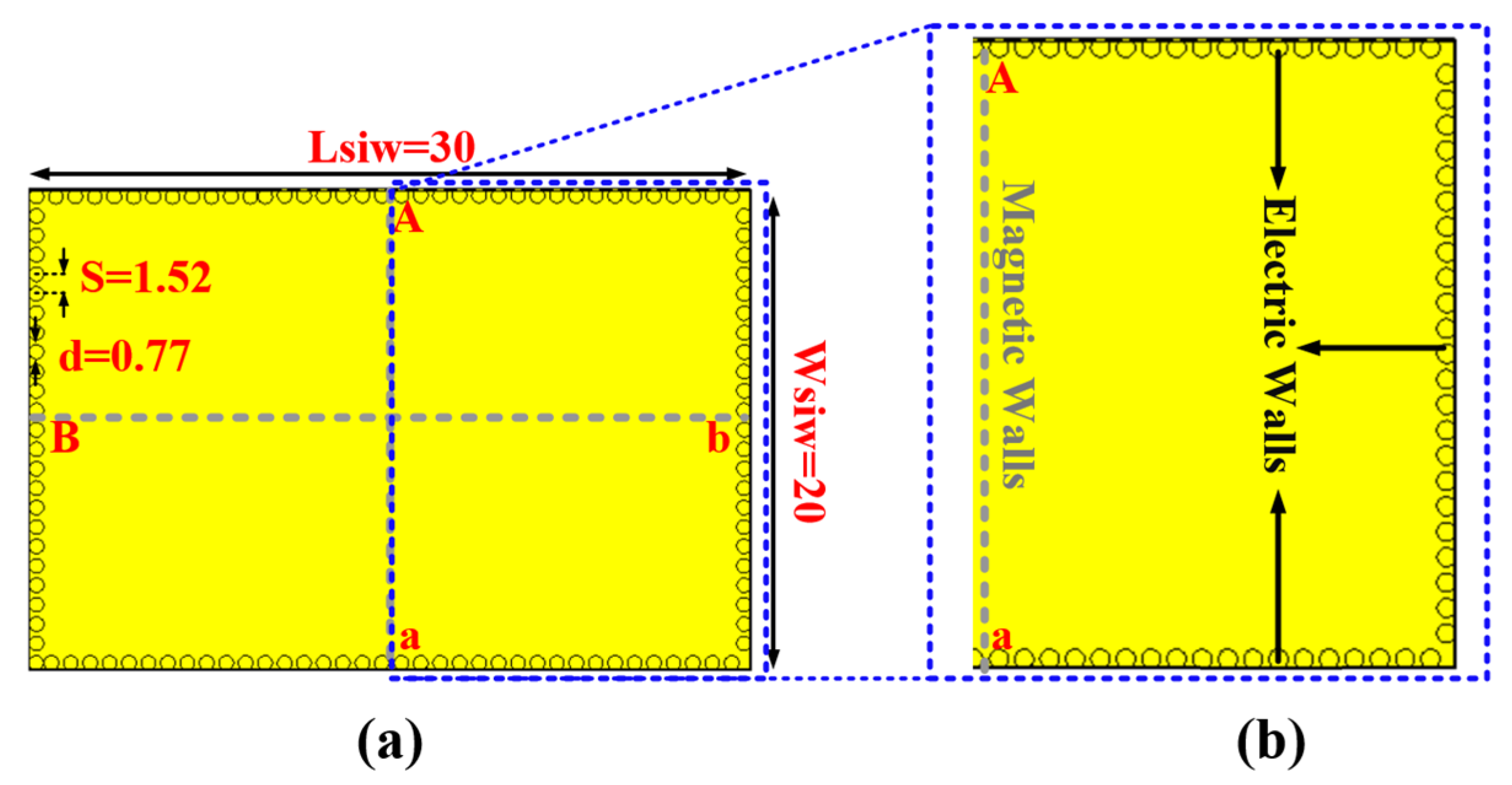
This research has taken steps toward realizing the proposed wireless sensor antenna with high sensitivity and accuracy. Therefore, the design process of the proposed wireless sensor antenna begins with the design of the antenna element, which refers to the HMSIW cavity. Thus, the evolution process of implementing the sensor antenna begins by designing a full-mode SIW (FMSIW) cavity structure to have a resonant frequency of its fundamental mode (TE110) at 6.2 GHz. The general geometry of the FMSIW is shown in Figure 2a, in which all design parameters are derived using Equations (1) and (2). It is worth noting that the SIW’s via parameters (s and d) are chosen carefully to avoid power leakage and to make sure the electric field is confined within the SIW structure [33].
d s 0.5
f T E 110 = 1 2 μ ε 1 W S I W 2 + 1 L S I W 2 ,   [ H z ]
where d represents via diameter, s represents the separation distance between vias, f T E 110 is the resonant frequency of the fundamental mode inside the FMSIW cavity, and W S I W and L S I W represent the width and length of the FMSIW cavity, respectively.
The eigenmode solver is deployed in the CST Microwave Studio to analyze the resonant mode’s frequency characteristics of the full-mode SIW cavity. As shown in Figure 3a, it has a full electric field distribution referring to the fundamental mode (TE110) frequency at 6.2 GHz. As can also be seen in Figure 3a, the electric field distributions are minimal near the via walls and strongly concentrated within the SIW cavity. Such a distinctive field distribution can contribute to boosting unique energy concentration and provide high levels of interaction situated within or in close proximity to the sensing area.
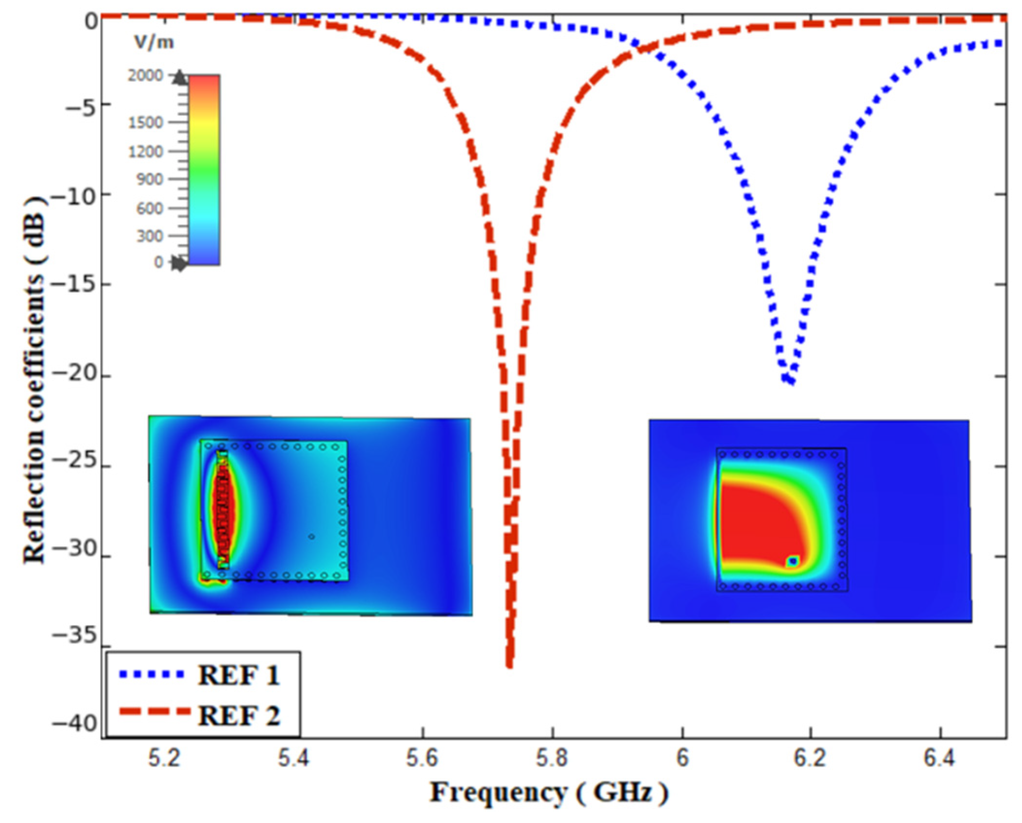
According to the symmetrical characteristics of the first order mode of the FMSIW, Figure 2a, a HMSIW cavity is created by dividing the FMSIW cavity along the magnetic walls (e.g., A–a), as shown in Figure 2b. One-half of the entire FMSIW cavity is highlighted in Figure 3b; it has a half cycle of the full mode and holds the same electric field characteristics of the TE110 at 6.2 GHz. This HMSIW cavity is excited using a coaxial cable to radiate the incident wave into free space through the magnetic wall, and is at a much smaller size (miniaturized design)—by about 50% of its full structure. The coaxial cable was selected as an appropriate option for the design due to its contactless capability, low power consumption, low cost, and ease of integration with circuits [24,33]. As depicted in Figure 4, the evaluation process of designing the sensor antenna begins with defining the HMSIW cavity, referring to REF 1.
In practice, the quality of the sensor antenna depends greatly on the sensing area. This area plays a significant role in determining the sensitivity and response of the sensor antenna to the alterations in the MUT. Thus, the implementation and creation of the sensing area depend on several parameters that must be considered, including (1) positioning it near the maximum electric field intensity and (2) enabling easy integration and cost-effective fabrication.
Creating a sensing area with a high-energy concentration can help increase the perturbation and interaction performance between the sensing site and the MUT. Typically, in the HMSIW cavity, the resonance and sensitivity properties predominantly rely on the electric field distribution between the open-end wall (the magnetic wall) and the ground. This region boasts the highest electric field intensity, rendering it an ideal selection for the sensing site. To this end, interdigital capacitor fingers are attached to the top surface of the HMSIW structure near the open-end wall (maximum electric field intensity); see REF 2, as shown in Figure 4. It is worth noting that the location of the interdigital fingers is precisely determined to capture the maximum electric field intensity, aligning with the open-ended wall area. Additionally, the size of the interdigital fingers (the width of the fingers and the distance between them) is optimized to tune the sensor antenna to operate efficiently at the desired frequency of 5.7 GHz. Selecting this frequency band enables the antenna to function within sub-6 GHz wireless communication bands.
In addition, such a configuration offers an array of shunt capacitors created between the fingers and the ground. This causes a larger capacitance, which contributes an increase in the energy stored in the sensing area. Consequently, any alterations in the dielectric properties within these specific regions can exert a notable influence on the sensor antenna response. Figure 5 shows the fundamental circuit model of the sensing area. C s is formed by the interdigital fingers and the ground and corresponds to the main sensing element, which is directly influenced by the dielectric permittivity of the integrated MUT [12]. L v is the inductance formed by the array of metallic vias, whereas C f   and L f form the conventional capacitance and inductance, respectively, from fingers themselves that correspond to the matching circuit, which does not vary with the MUT.
Figure 6 shows the simulated reflection coefficient for REF 1 and REF 2 antennas. It is can be seen that the HMSIW cavity (REF 1) resonates at 6.2 GHz, matching the resonance frequency of the TE110-mode FMSIW. This confirms our claim in which the ministered cavity holds the same electrical characteristics of the full structure. In the REF 2 antenna, the resonance frequency is shifted down to 5.7 GHz, which is due to the increasing capacitive effect that results from integrating the interdigital capacitor configuration. Furthermore, it can be seen that the resonance frequency of REF 2 has a deeper matching level; this is attributed to the fact that the HMSIW cavity stores a large amount of energy resulting from the capacitor structures in the sensing area. Figure 6 also depicts the simulated electric field distribution for REF 1 and REF 2 at the sensing area. This figure demonstrates that REF 2 exhibits a high field, with energy symmetrically concentrated along the open-ended line of the HMSIW. This characteristic makes REF 2 a favorable option for the proposed sensor antenna compared to REF 1.
Since the interdigital capacitance HMSIW cavity (REF 2) shows a good agreement between compact size and high energy concentration, it is used in the resonator section of the sensor. Thus, the proposed sensor antenna (REF 3) [Figure 4] is launched by integrating a microfluidic channel loaded with a water sample at a room temperature of 25 °C in the sensing area, which is placed exactly below the interdigital capacitor configuration. An interaction is then created in the region with the highest electric field, leading to a significant perturbation in the effective permittivity of the water sample. In addition to creating a strong field in the sensing area, the microfluidic channel provides a uniform distribution and excessive pressure to the water sample in the sensing area, making the high field and energy interact uniformly with the water sample. The errors that occur would be largely prevented, which would increase the sensor sensitivity.
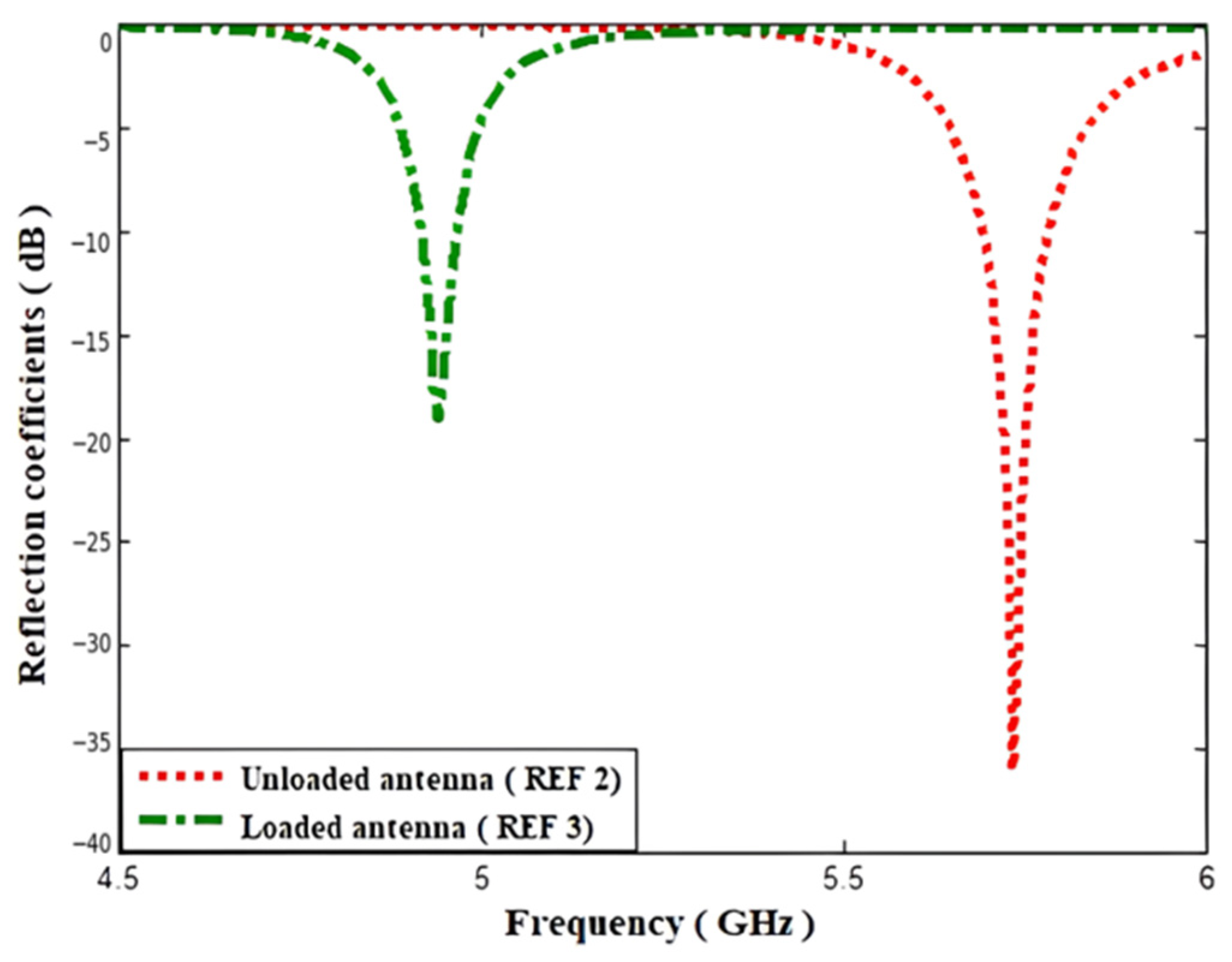
After integrating the PDMS layer and loading the microfluidic channel with the water sample, the detection process is launched by examining the variation in the effective permittivity with changes in the water’s temperature. It is worth noting that the PDMS layer does not influence the performance of the sensor antenna, as the electric properties of both substrate and PDMS layer are the same ( ε P D M S ε S u b 2.7 ). When the water sample is piped and comes into contact with the sensing area, the propagated electromagnetic waves penetrate the water sample, disturbing the electric fields. Now, due to the increase in the effective permittivity ( ε w a t e r ( 25   ° C ) = 78.6 ) at the sensing area, the sensor reflection response will change. Figure 7 shows the simulated refection coefficient for both REF 2 (unloaded sensor) and REF 3 (loaded sensor)—it can be seen that the resonance frequency of REF 2 is shifted down to 4.9 GHz when the effective permittivity increases. Additionally, Figure 7 demonstrates that the proposed sensor antenna (REF 3) sustains a stable matching level. This stability is credited to the robustness of REF 2, which efficiently maintains a high matching level to counteract the high losses resulting from the high effective permittivity. It is concluded that changing the resonance frequency serves as evidence of the antenna’s sensitivity and its ability to adapt to variations in the characteristics of the sensing area, thereby enabling accurate detection of changes in the water sample’s permittivity.

2.3. Description of Sensor Performance during Loading

As has become clear, the sensing principle of the proposed sensor is to change the resonance frequency created by loading the water sample into the sensing area. The performance of the sensor antenna is defined based on changing the capacitance at the sensing site, which results from electric field interaction with the MUT. Increasing the sample’s permittivity shifts the resonance frequency downward and shows a linear variation in the resonance frequency of the sensor. This correlation can be obtained using Equations (3) and (4), which show the relationships between the (effective permittivity and capacitance) and (capacitance and resonance frequency), respectively. In these equations, ε e f f   is the effective permittivity of water (representing the   C s material), A   is the capacitor plate area, and h c represents the distance between the plates, which corresponds to the antenna’s thickness. As mentioned earlier, this thickness plays a crucial role in selecting the operating frequency and determining the physical performance, such as antenna size. Additionally, the thickness governs the interaction between the EF and the MUT. Increasing the thickness of the antenna layer ( h c ) leads to an increase in capacitance (Cs), which, in turn, decreases the coupling and interaction of the EF with water [12].
  C s = ε e f f A h c
F 0 = 1 2 π L C s
In order to understand the validity of this structure as a temperature sensor, it is necessary to provide some information about the relationship between the dielectric permittivity of water and its temperature. This correlation is obtained from Equation (3), where it is shown that as the water permittivity decreases, the water temperature increases. Here, it can also be said that the change in the temperature of the water sample leads to a change in effective permittivity of the sensing area, which changes its effective permittivity. As a result, the resonance frequency of the sensor shifts. From this change in resonance, it can be deduced that the water’s temperature level has changed. The investigation of the sensing characteristics is carried out in the following manner:
  • Employ samples with diverse water temperatures ( T w a t e r ), ranging from 0 °C to 50 °C, for classification into frost and wildfire monitoring purposes.
  • Calculate the variation in the effective permittivity with the addition of each water sample’s temperature degree. This is achieved by calculating the dielectric constant of water over the range from 0 °C to 50 °C using Equation (5) [30]. This provides an approximation for calculating the effective permittivity of water based on the water temperature change in degrees:
      ε e f f = 87.740 0.40008   T + 9.398 × 10 4   T 2 1.410 × 10 6   T 3
    where ε e f f is the effective permittivity of the water and T is the temperature in degrees Celsius. In our case, ε 25   ° C   = ε R o o m   T e m p e r a t u r e = 78.6, ε 0   ° C   = ε f r o s t   = 87.740 , and ε 50   ° C   = 67.736, while ε I c e   = 3.2 (at temperature below 0 °C). The sensor’s antenna response can be described as follows: f / ε = 5.5 MHz/ε, and, f / c = 1.83 MHz/°C.
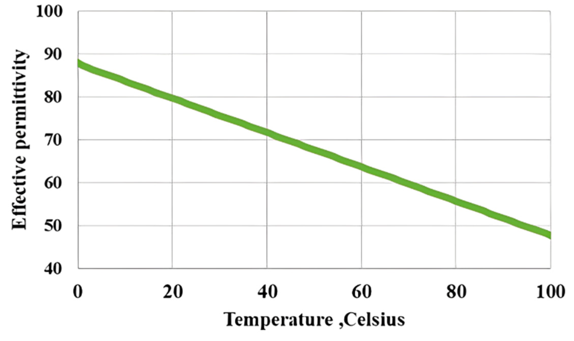
  • Investigate the relationship between the resonance frequency and water temperature. This is achieved by examining the relationship between the effective permittivity and water temperature at each degree. Figure 8 demonstrates that the effective permittivity increases with a decrease in water temperature (linear regression). On the other hand, the resonance frequency shifts downward with a decrease in water temperature, corresponding to an increase in effective permittivity, as shown in Figure 9a, demonstrating that the antenna sensor is able to distinguish medium temperatures from low to high; this reflects the ability of this design to detect and forecast frost and wildfires over the sensing region at an early stage. Furthermore, this sensor is capable of distinguishing the presence of ice when ε I c e   = 3.2, as shown in Figure 9b. Meanwhile, the simulated return loss displays a high sensitivity to water temperature changes over the sensing region and to the presence of ice. However, the antenna’s resonance frequency response is more reliable because the resonance frequency is not sensitive to the losses between the sensor antenna and the receiver side. In contrast, the resonance amplitude would be significantly impacted by the distance between two transmitting and receiving antennas. Table 1 presents the simulated resonance frequency with respect to each water sample’s temperature.

3. Far-Field Performance

To confirm our claim regarding the ability of the proposed sensor antenna to sense while simultaneously transmitting its sensing results, the far-field parameters in terms of total efficiency and peak gain are explored and examined in this subsection. As illustrated in Figure 10, the first-order mode of the HMSIW antenna sensor has a superior radiation efficiency and gain at 5.7 GHz (unloaded). Furthermore, Figure 11 shows that the proposed sensor antenna can sense and transmit the sensed results at the same time, where the antenna sensor radiates power with different amplitudes at different recorded resonance frequencies within the sensing temperature range, resulting in the reception of different signals at different temperatures. Moreover, the antenna sensor has stable far-field performance and the ability to radiate power even while the effective permittivity increases. In addition, the sensor can still operate within the UWB band, ensuring its reliability in transmitting sensed results. This is due to the use of an annotative combination of SIW and microscale water samples to prevent radiation losses. Based on the far-field results, the proposed antenna sensor has the full ability to monitor and detect the medium’s temperature in a wide sensing range with low cost and in real time, along with the additional advantages of wireless capability, which eliminates the need for long transmission lines in large structures.
Figure 12 displays the 2D comparison of the XY and XZ normalized far-field radiation patterns of the HMSIW sensor antenna at 5.7 GHz. Both patterns exhibit directional characteristics similar to the slotted SIW antenna. This supports what was mentioned previously, namely, that the interdigital capacitor slot concentrates the electric field disruptions. Furthermore, these patterns prove our claim that the sensor acts as an antenna by showing effective results in the far-field region. Finally, this study proves that the proposed design works as both a sensor and an antenna at the same time.

4. Proposed Smart Sensor Antenna

4.1. Problem Description

As observed in the previous section of the sensor antenna results, the differences between the near and far-field parameters, including resonance frequency, total radiation efficiency, and gain, all depend on the dielectric constant of water. This, in turn, will vary with changes in the degree of the water’s temperature. However, recording the simulated sensor results manually and using relevant mathematical formulas is not suitable for interpolation tasks, especially when dealing with non-linear behavior and unpredictable intervals. Such mechanisms cannot effectively capture the underlying smoothness in the data and provide unreliable predictions. This can be considered a disadvantage when dealing with small intervals in data points, where the estimations between closely spaced data points become crucial and uncertain. To mitigate this, machine learning (ML) can adapt to changes in the environment and weather conditions over time. ML offers several advantages for modeling the resonance frequency and detecting weather conditions such as frost, normal conditions, or wildfire, including its ability to capture non-linear behavior, its robustness to small shifts, and flexibility in selecting multiple detecting parameters (features), which allow for accurately characterizing the complex relationship between the features and weather conditions. Furthermore, the estimations provided by ML can help to quantify the confidence in the predictions and decision-making process, thereby improving the model’s ability to accurately classify any new data points related to weather conditions. In this paper, we present several machine learning models to estimate and classify the weather conditions into three types (frost, normal, and wildfire), instead of the typical use of analytical formulations and manual observation.
Let X = [ x 1 ,   x 2 , ,   x N x   ] denote an input feature vector where N x is the number of features considered. Our inputs consist of N x = 3 features, namely: the center frequency f c (resonance frequency), and the lower and upper frequencies ( f l   ,     f u   ) of −3 dB S 11 . In this paper, the inclusion of multiple frequency parameters adds redundancy to the model, making it more resilient to noise or measurement errors. If one parameter is affected by interference or inaccuracies, the model can still rely on the other parameters for accurate predictions. Furthermore, by incorporating all of the three parameters, the prediction window expands because the model has more data points and factors to consider. Each feature provides additional information that helps the model capture more complex patterns and relationships within the data. As a result, the model can explore a wider range of possible outcomes, increasing the flexibility and depth of predictions. Using these features can enhance certainty by confining the estimation results within the prediction area; for example, any new frequency points ( f l   ,   f c ,   a n d   f u ) located within this interval can provide estimations of the confidence level in the anticipated outcomes, enabling us to present the forecast results with greater accuracy and reliability. In contrast, when using a single feature, the model has limited information, and must rely solely on that feature for predictions. This constraint causes the model to predict new values that are close to the given feature’s known range, limiting the variability of outcomes. It is worth noting that all features (frequencies) have the same impact on weather detection. Each of these frequencies is similarly affected by changes in antenna permittivity, ensuring that they contribute equally to the detection process. This consistency in response supports the reliability of the system for accurately identifying weather conditions.
Let Y represent the output target single class indicating weather conditions: frost, normal, or wildfire. This classification task involves several steps: Firstly, the weather temperature ranging from 0 °C to 50 °C is categorized into three ranges: (0 °C to 6 °C), (7 °C to 30 °C), and (31 °C to 50 °C), corresponding to Early Frost (EF), Normal (N), and Early Wildfire (EW) conditions, respectively. These classifications of the environmental state were identified mainly in order to obtain an early detection characteristic, in addition to the various factors unique to each category. Frost is usually expected to occur at around 0 °C [17]. However, for early frost detection systems, the temperature threshold is typically set just above this temperature. Depending on the specific crop, location, and climate in question, frost can start forming even slightly above this point, so systems are often designed to detect temperatures around 0–5 °C [46]. The 0–6 °C range is selected as the threshold temperature range in order to guarantee detection at an early stage. In the case of wildfire, the temperature threshold is selected as 30–34 °C. This selection is mainly influenced by the 30–30–30 rule, which states that a temperature above 30 °C, humidity less than 30%, and wind speed above 30 kmph together indicate extreme fire risk [47]. A normal status refers to temperatures that are higher than the threshold for frost formation but lower than those that would trigger wildfire risks. By choosing water as the material under test, we are able to achieve a broader sensing range. This significantly enhances our model’s predictive capabilities, facilitating earlier detection of temperature variations from 0 to 50 °C and above, which is crucial for timely interventions. Unlike previous studies—which often used materials with restricted sensing ranges, either confined to very high or very low temperatures—our approach allows for more versatile monitoring across a wider spectrum of conditions. Within these ranges, the effective permittivity is calculated. Subsequently, a simulation process is initiated to identify the resonance frequencies (features: f l   ,   f c ,   a n d   f u   ) associated with each class (outputs: EF, N, and EW). This methodology enables the early estimation of disaster conditions, thereby facilitating proactive responses.

4.2. Data Generation and Preparation

For the present study, two classification supervised ML approaches (labeled data) are applied to extract the patterns mapping from X to Y that can then be used for the platform. This allows for an estimation of weather conditions without relying on tedious analytical and mathematical formula approaches. The initial classification model adopts the perception-based approach using artificial neural networks (ANNs), while the subsequent model employs the non-parametric approach, leveraging widely used machine learning models, such as random forest, support vector classification (SVC), and Gaussian process (GP) classification. The ML model used in this design relies mainly on ANNs, as other models were used to validate the sensor antenna detection performance. ANNs offer significant advantages over other machine learning models due to their ability to handle complex, non-linear relationships and their scalability. Unlike other models, ANNs automatically learn important features from the data without requiring extensive feature engineering. This is especially beneficial in applications where manual feature extraction might be challenging. Furthermore, the multi-layer structure of ANNs allows them to learn hierarchical features, making them effective for tasks where relationships between variables are not straightforward. In order to train our proposed ML models, a dataset of 280 samples was generated by simulating the proposed sensor antenna at the calculated effective permittivity across the three previously mentioned temperature ranges using the CST Microwave Studio software 2019. Each sample in the dataset consisted of the resonate frequency parameters (numerical), which were used to predicate and classify the weather conditions (categorical).
In order to obtain an effective ML model that can make accurate predictions, the dataset was prepared before the training process. To this end, we employed the standard scaling statistical model to normalize the input values, ensuring consistency and comparability across features. Additionally, we utilized the one-hot encoding technique to convert the three categorical classes into numerical representations, enabling the machine learning algorithms to effectively process and analyze the categorical data. After preparing the dataset, the training process was launched by splitting the labeled data samples, which contain the frequencies (scaled values) and weather condition states (encoded values). The sizes of the training samples were split based on the ML model’s requirements (as described later), in which these samples were used to train the ML models to capture the pattern between the frequencies and weather conditions. During the training, each model learns the patterns by adjusting its parameters. For example, a model like an ANN learns by adjusting weights during each pass-through of the data (using backpropagation) and improves its predictions based on the error rates (using a loss function). In contrast to other models, in RF, several decision trees are created using subsets of the data, and the results are aggregated for a final prediction. On the other hand, the SVC model attempts to find a hyperplane that best separates the classes, adjusting based on data points that are difficult to classify. The Gaussian process model learns by fitting the data into Gaussian distributions, providing probabilistic predictions rather than deterministic outputs.
After that, the monitoring process is guided by receiving the frequency values f l   ,   f c ,   a n d   f u   on the receiver side. The machine learning model is designed to capture any new incoming values of f l   ,   f c ,   a n d   f u   that fall within a predefined temperature range: (0–6 °C), (7–30 °C), or (31–50 °C). These values are then analyzed by the model to accurately identify the corresponding environmental condition, whether it is low (such as early frost) or high (such as wildfire conditions). The system ensures that frequencies associated with particular weather states are effectively recognized, thus minimizing the likelihood of confusing one condition with another (e.g., a low likelihood of frost detection during an active wildfire). This tailored monitoring approach allows for precise predictions based on real-time observed frequencies.

5. Proposed Machine Learning Approach

In the subsequent sections, we introduce two distinct approaches aimed at augmenting the reliability and assurance of the proposed intelligent sensor antenna. By incorporating various machine learning methodologies, we aim to bolster the decision-making capabilities of the sensor system, ensuring enhanced detection accuracy and confidence in its outputs. To this end, the perception-based approach using an ANN model is presented and mathematically described in this section. In addition, non-parametric-based approaches using the other models are adopted as validation models.

5.1. Perception-Based Approach

This approach falls within the realm of machine learning, specifically deep learning, utilizing a neural network model known as an ANN. Modeled after the computational principles of the human brain, ANNs comprise interconnected neurons, enabling them to perform complex computations and pattern recognition tasks. ANNs’ capability for forward and backward propagation facilitates the mapping of inputs to outputs while allowing self-error correction, making them well-suited for applications requiring forecasting and predictive analysis [44]. There are many different ANN structures used in the literature. Multilayer perceptrons (MLP s) [48,49,50,51,52,53,54], which are successfully and commonly employed in engineering problems, are preferred in this study because of their ability to learn and model complex patterns.
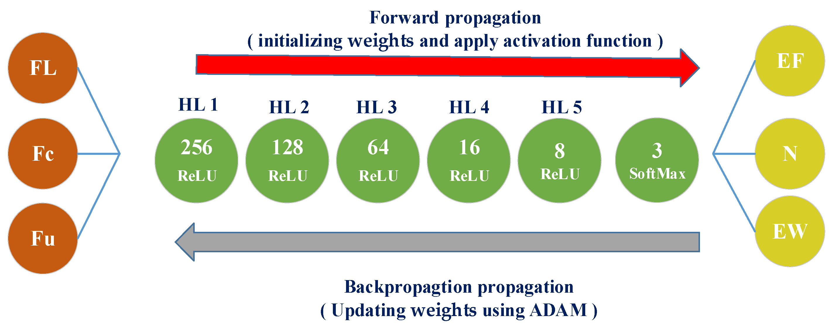
The architecture of the ANN we developed for disaster forecasting is further described in Table 2 and Figure 13 in terms of the number of layers, units, training hyper-parameters, and choice of activation. The network consists of an input layer that includes three input parameters. The input layer then feeds into several fully connected hidden layers, with decreasing numbers of hidden neurons activated using the Rectified Linear Unit (ReLU) function. It is important to note that the selection of the number of layers and neurons in the model is carefully tuned to achieve optimal accuracy and performance in the ANN. This tuning process ensures that the network is neither too simple, which might lead to underfitting, nor too complex, which could result in overfitting, thereby maximizing the model’s predictive capabilities. The final layer is a Softmax multi-label classification that predicts weather conditions. The regular feedforward operation in fully connected ANNs is given by the following equation:
v j = Z i w i j u i + b j ,  
where j represents the layer index, i represents the neuron index, v j is the output that adds up the input signals u i   after multiplying by weight w i j and adding the bias b j , and Z   represents the chosen activation function. The neural network’s weight vectors are initialized using Glorot normal initialization, which calculates the variance of weights based on the number of input and output units for each layer. This technique aims to ensure stable and efficient training by sampling weights from a Gaussian distribution with zero mean and the calculated variance, facilitating effective learning during training.
In this study, the MLP can be trained using the backpropagation (BP) mechanism, which is one of the primitive training mechanisms for neural networks. In our analysis, the generated dataset is split into 70% training, 10% validation, and 20% testing, using a random seed of 70. The ANN model is developed using the Tensorflow library [28] and trained using the adaptive moment estimation (ADAM) algorithm. The network is trained to minimize categorical cross entropy (CCE) as a loss function, which is given by [44]
C C E = 1 n   i = 1 n j = 1 m y i j l o g ( ŷ i j )
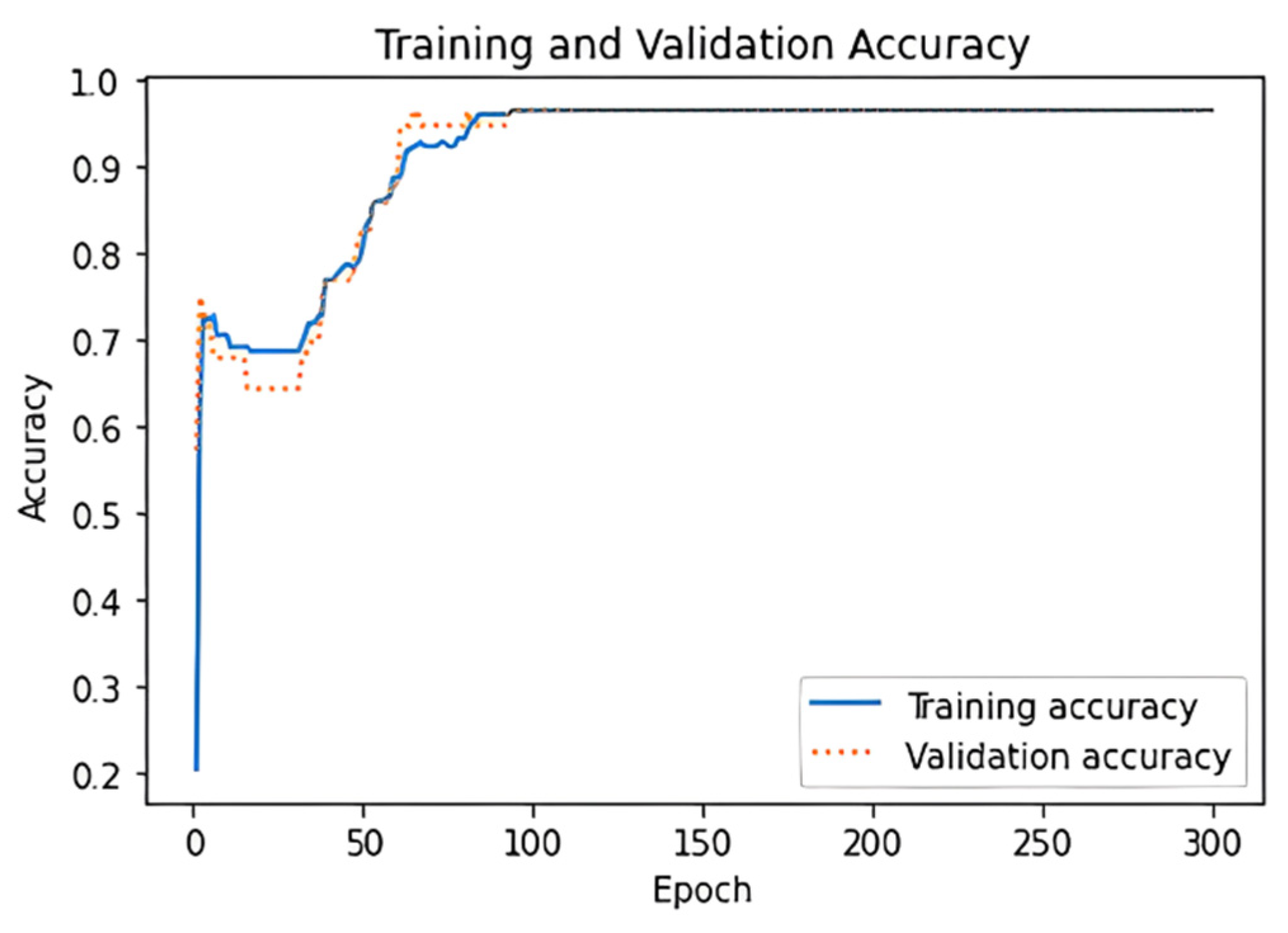
In the ANN model, the training process is launched by passing the training data samples through the network, layer by layer (forward propagation), with the ReLU activation function applied to introduce non-linearity. This non-linear relationship helps the model to capture complex patterns between the input features and the target outputs, enabling it to learn more sophisticated relationships within the data. Predictions are then made based on the current weight, and the error between predicted and actual outputs is computed using categorical cross entropy. After that, backpropagation adjusts the weights to minimize the error by calculating the gradient of the loss function with respect to each weight, and the Adam optimization algorithm updates the model’s parameters. Such a process happens over multiple epochs, where the entire training dataset is passed through the model several times in smaller batches to speed up learning. For each batch, weights are updated to minimize the error. To that end, minimizing the loss function and tuning the performance on the validation set is optimized via a process of obtaining the hyper-parameter: the number of neurons, the activation function, the weight initialization technique used in the hidden layer, and the number of epochs. Figure 14 depicts the evaluation process of both the training and validation sets. It illustrates that the model consistently demonstrates stable and commendable performance across 300 epochs. This stability suggests that the model is effectively learning the patterns present in the data and is not overfitting. Consequently, the model appears to have successfully captured the underlying relationships within the training data while generalizing well to unseen data, as evidenced by its performance on the validation set. This indicates a normal fitting process, implying that the model is adequately prepared and capable of handling the testing set.

5.2. Non-Parametric-Based Approach

This subsection presents the most popular non-parametric ML algorithms for classification tasks. Such algorithms do not make explicit assumptions about the functional form of the relationship between features and targets, allowing for flexibility in handling the complex data distribution. Instead, this approach uses techniques like kernel smoothing or use decision boundaries to approximate the underlying distribution of the data [51]. This enables the modeling of intricate interactions in a more adaptable manner, without relying on preexisting knowledge. In pursuit of accurate weather forecasting, three distinct models—random forest (RF), support vector machine (SVM), and Gaussian process (GP)—have been meticulously developed and implemented for validation purposes. Each model serves as a validation tool, contributing to a robust and reliable forecasting framework. The random forest model operates by constructing an ensemble of decision trees, utilizing bootstrapped subsets of the data and random feature selection to ensure diversity and robustness. The support vector machine model, on the other hand, seeks optimal hyperplanes to separate different weather patterns in a high-dimensional feature space. Finally, the Gaussian process model leverages probabilistic distributions to model the uncertainty inherent in weather predictions, offering insights into the confidence levels associated with forecasted outcomes. Together, these models collectively bolster the accuracy and certainty of weather forecasts, providing invaluable insights for various applications and decision-making processes. In these models, the generated dataset is split into 80% training and 20% testing, using a random seed of 70.

5.2.1. Random Forest (RF)

Random forest is an ensemble learning method that constructs multiple decision trees during training. Each decision tree is constructed on a random subset of the training data and a random subset of features. The final prediction of the random forest is determined and estimated by aggregating or voting on the predictions of individual trees [51]. For classification tasks, this aggregation is typically achieved by taking the mode of the predicted classes among all the trees.
Mathematically, let us denote our dataset as D = {(x1, y1), (x2, y2), …, (xN, yN)}, where x i represents the features and yi represents the corresponding labels. RF constructs M decision trees, where each tree Tm is trained on a bootstrap sample Dm of the original dataset. Additionally, at each node of the tree, a random subset of features Fm is selected to determine the best split. The final prediction of the RF ŷ for a new instance x is obtained by aggregating the predictions of all trees:
y ^ = m o d e ( T 1 ( x ) ,   T 2 ( x ) ,   ,   T M ( x ) )

5.2.2. Support Vector Classification (SVC)

Support vector machine is a supervised learning algorithm that estimates the optimal hyperplane in the feature space to separate different classes and is capable of performing linear or nonlinear classification, and even outlier detection. In a multi-classification scenario, SVM aims to find the hyperplane with the maximum margin between the nearest data points of different classes, known as support vectors [54]. The loss function of the SVC algorithm is given by
J   ( w ,   b ) = 1 2 w T w + C   i = 1 m max 0,1 t i w T x i + b  
The first sum in the cost function will push the model to have a small weight vector w , leading to a larger margin. The second sum, which contains the function m a x ( 0 , 1 t i ), is called the hinge loss function, and C is the regularization term. In this study, we use the linear function as the kernel, and C is selected to be 20.

5.2.3. Gaussian Process (GP)

The Gaussian process is a supervised machine learning probabilistic classification approach renowned for its high accuracy, robustness, and interpretability [52]. It excels in identifying the most relevant features while effectively handling noisy data, ensuring reliable classification performance. The GP has a number of advantages, including the fact that it can produce satisfactory findings even when working with a restricted collection of data, as well as its ability to provide measures of ambiguity for predictions. The GP adopts the Radial Basis Function (RBF) to estimate its predictions and provides a measure of certainty or confidence in its classification decisions, as given below:
k ( x , x ) = σ 2 e x p ( x x 2 2 σ 2 )
where x x 2 represents the squared Euclidean distance between x and x′, σ is the length scale parameter, which controls the “width” of the kernel and determines how quickly the similarity between data points decreases with distance.

6. Performance Measurement Metrics

The performance of the models is evaluated using the statistical metric widely used in the evaluation of classification models, which is the accuracy score [55]. The accuracy score measures the proportion of correctly classified samples out of the total number of samples. It is commonly used as an evaluation metric in classification tasks to assess the overall model performance:
A c c u r a c y = N u m b e r   o f   c o r r e c t   p r e d c t i o n s T o t a l   n u m b e r   o f   p r e d c t i o n s  

6.1. Performance on the Test Set

The performance of various models, including artificial neural networks (ANNs), random forests (RF), support vector classification (SVC), and Gaussian processes (GP), was evaluated on the test set, and the results were achieved with an accuracy of 96.2%. It is evident that all models exhibit remarkable predictive accuracy, boasting an impressive score of 96.4%. Notably, the ANN model demonstrates not only high accuracy but also robust generalization capabilities, as it performs well on data points beyond those encountered during training and validation, indicating resilience against overfitting.
Moreover, the outcomes obtained from RF, SVC, and GP models corroborate the effectiveness of ANNs in forecasting weather conditions. These findings underscore the reliability of the sensor antenna in estimating and predicting weather conditions for unseen data points. This suggests its potential utility in real-world applications, where accurate weather forecasting is paramount.

6.2. Performance on the Test Set Examples

In order to thoroughly assess the efficacy of the ANN alongside other algorithms, a meticulous validation process was conducted. This involved randomly selecting three samples from the test set and employing the models for inference to predict the weather conditions. Notably, the chosen samples were deliberately diverse, representing temperatures of 6 °C, 8 °C, and 33.8 °C, denoted as EF, N, and EW, with closely matched effective permittivity values of 85.3, 84.5, and 74.2, respectively. This deliberate selection aimed to simulate scenarios where the frequencies for both samples closely align, thereby presenting challenges for accurate decision-making and predictions. These samples were then used to simulate the proposed sensor antenna using CST in order to compare the CST results (actual) and ML results (predicted). This validation process involves several steps: (1) Sample selection: randomly select samples from each temperature category (6 °C, 8 °C, and 33.8 °C). (2) Effective permittivity calculation: calculate the effective permittivity for each sample using the aforementioned formula. (3) Sensor antenna simulation: simulate the proposed sensor antenna by changing the water permittivity. (4) Detecting parameter recording: record relevant detecting parameters from the simulation results. These parameters can be chosen from either the near-field or far-field data. (5) Use the recorded detecting parameters to predict the weather conditions using the machine learning model.
Upon analysis, the results depicted in the accompanying Table 3 reveal a striking alignment between the predicted values and the actual observations. This remarkable coherence underscores the sensor antenna’s adeptness in discerning weather conditions even amidst subtle shifts. Such findings serve to bolster our assertion regarding the sensor antenna’s prowess as an intelligent system capable of extracting nuanced weather patterns, thereby reinforcing its utility in diverse real-world applications.

7. State-of-the-Art-Comparison

For the purposes of proving the validity of the proposed design, in this section, previously published studies are compared with the proposed sensor antenna design for environmental temperature and weather conditions applications in terms of the antenna/resonator configuration, material under test (MUT), parameter under test (PUT), detection methodology (DM), and machine learning (ML). As is shown in Table 4, our proposed design is the first to monitor a wide range of temperatures for ice, frost, and wildfire conditions using multiple detecting parameters in conjunction with machine learning, unlike previously published sensor antennas that focus solely on high or low temperatures, using only a single detection parameter. Additionally, our design requires only a 50-μL water sample with microfluidic technology, compared to others that rely on solid materials and ice accumulation for detection. Moreover, we adopt an innovative approach by incorporating substrate-integrated waveguide (SIW) and interdigital capacitor techniques, which have not been used in previous studies that typically utilize traditional antenna types. Finally, there is no existing study that addresses real-world applications requiring sensor antennas for temperature monitoring, particularly for scenarios where temperature fluctuations can significantly impact performance.

8. Conclusions

This paper introduced an innovative microwave antenna sensor that integrates a microfluidic channel and a half-mode substrate-integrated waveguide cavity (HMSIW) to detect natural disasters caused by frost and wildfire through the monitoring of the temperature of microliter water at 5.7 GHz. The incorporation of a microfluidic channel and the TE101 mode HMSIW resonator allows for significant perturbations in the effective permittivity of the integrated water sample. The performance of the sensor was evaluated by investigating the behavior of dielectric permittivity changes as the 50-μL water temperature changes in a wide sensing range from a sample. The outcomes showed the resonance frequency’s excellent sensitivity, with changes of ∆f/∆ε = 5.5 MHz/ε and ∆f/(∆°C) = 1.83 MHz/°C, making it possible to precisely identify frost and wildfire disasters. Furthermore, the proposed design was confirmed in its ability to transmit the sensed data. This is supported by its excellent far-field performance at different water temperatures. To enhance decision-making capabilities and imbue the sensor system with cognitive abilities, several classifier-based machine learning techniques—such as artificial neural networks (ANNs), random forests (RF), decision trees (DT), support vector machines (SVMs), and Gaussian processes (GP)—were investigated. Such techniques were used to predict and classify environmental temperature levels into one of three environmental states (Early Frost, Normal, Early Wildfire), with an accuracy of 96.4%. Based on the results obtained in this study, it can be concluded that a machine learning approach is essential for frost and fire detection due to its ability to handle complex, dynamic environmental data in real time. It can adapt to various conditions, offering higher accuracy and reducing false alarms.

9. Future Work

According to the results obtained and the comparisons made with similar studies, the proposed RF sensor antenna may be a good candidate for use in temperature monitoring systems due to its many advantages, such as noninvasiveness, compactness, ease of integration and fabrication, low cost, low power consumption, and high sensitivity. But, as mentioned, this work represents a fundamental step in our ongoing research, and there are many steps ahead of us leading up to the commercialization stage and providing more solutions for smart grid systems. The proposed sensing antenna offers significant contributions to smart grid technology. Beyond tracking and detecting heat, it can perform additional tasks, such as harvesting energy using radio electromagnetic waves. This energy can be harvested from the main station or through other distributed sensing points within the smart grid. By integrating this antenna, smart grids can enhance their efficiency and resilience. The dual functionality of monitoring environmental conditions and energy harvesting not only optimizes energy management, but also provides a sustainable solution for powering distributed sensors and devices, contributing to a more reliable and robust smart grid infrastructure. Furthermore, integrating the proposed sensor antenna along with machine learning into the smart grid can provide a dynamic approach to maximize power efficiency; for example, solar panels can be oriented based on sunlight intensity (high temperature) predictions.

Author Contributions

Conceptualization, A.T.A., R.A. and J.Z.; methodology, A.T.A. and R.A.; software, A.T.A.; validation, A.T.A., R.A. and J. Z; formal analysis, A.T.A. and R.A; investigation, A.T.A. and R.A; resources, A.T.A.; data curation, A.T.A.; writing—original draft preparation, A.T.A.; writing—review and editing, A.T.A., R.A. and J. Z; visualization, A.T.A.; supervision, R.A.; project administration, R.A.; funding acquisition, R.A. and J.Z., All authors have read and agreed to the published version of the manuscript.

Funding

This research was funded by the North Atlantic Treaty Organization (NATO)/Science for Peace and Security (SPS), funder reference SPS G5932, project reference WT 433209.

Data Availability Statement

The data presented in this study are available on request from the corresponding authors.

Acknowledgments

We would like to thank the funder (NATO/SPS) in addition to Mutah University and the University of Liverpool for the support of this work.

Conflicts of Interest

The authors declare no conflicts of interest.

References

  1. Zhou, I.; Lipman, J.; Abolhasan, M.; Shariati, N.; Lamb, D.W. Frost monitoring cyber–physical system: A survey on prediction and active protection methods. IEEE Internet Things J. 2020, 7, 6514–6527. [Google Scholar] [CrossRef]
  2. Calfire. Cal FIRE. Available online: https://www.fire.ca.gov/ (accessed on 21 August 2024).
  3. Wei, K.; Yang, Y.; Zuo, H.; Zhong, D. A review on ice detection technology and ice elimination technology for wind turbine. Wind. Energy 2020, 23, 433–457. [Google Scholar] [CrossRef]
  4. Red Cross. The Climate Crisis: Why the World Must Act Now. Available online: https://www.redcross.org.uk/stories/disasters-and-emergencies/world/the-climate-crisis (accessed on 2 July 2024).
  5. The National Center for Security and Crisis Mangament (NCSCM). Jordan National Natural Disaster Risk Reduction Stratagy. 26 March 2019. Available online: https://www.preventionweb.net/files/68511_nationalnatrualdisasterriskreduciot.pdf (accessed on 2 July 2024).
  6. Kobziar, L.N.; Thompson, G.R. Wildfire smoke, a potential infectious agent. Science 2020, 370, 1408–1410. [Google Scholar] [CrossRef]
  7. National Weather Service. Wildfire Information and Safety Rules. Available online: https://www.weather.gov/otx/Wildfires (accessed on 2 July 2024).
  8. Somov, A. Wildfire safety with Wireless Sensor Networks. ICST Trans. Ambient. Syst. 2011, 11, e4. [Google Scholar] [CrossRef]
  9. Oolin, D.M.; Sitar, N. Wireless sensors forwildfire monitoring. In Proceedings of the Conference on Sensors and Smart Structures Technologies for Civil, Mechanical, and Aerospace Systems, San Diego, CA, USA, 7–10 March 2005; pp. 477–484. [Google Scholar]
  10. Leblon, B. Monitoring forest fire danger withremote sensing. Nat. Hazards 2005, 35, 343–359. [Google Scholar] [CrossRef]
  11. Jiang, X.; Taneja, J.; Ortiz, J.; Tavakoli, A.; Dutta, P.; Jeong, J.; Culler, D.; Levis, P.; Shenker, S. An architecture forenergy management in wireless sensor networks. ACM Sigbed Rev. 2007, 4, 31–36. [Google Scholar] [CrossRef]
  12. Ebrahimi, A.; Beziuk, G.; Scott, J.; Ghorbani, K. Microwave diferential frequency splitting sensor using magnetic-LC resonators. Sensors 2020, 20, 1066. [Google Scholar] [CrossRef]
  13. Su, L.; Muñoz-Enano, J.; Vélez, P.; Gil-Barba, M.; Casacuberta, P.; Martin, F. Highly sensitive refective-mode phase-variation permittivity sensor based on a coplanar waveguide terminated with an open complementary split ring resonator (OCSRR). IEEE Access 2021, 9, 27928–27944. [Google Scholar] [CrossRef]
  14. Malyuskin, O. Microplastic detection in soil and water using resonance microwave spectroscopy: A feasibility study. IEEE Sens. J. 2020, 20, 14817–14826. [Google Scholar] [CrossRef]
  15. Jha, A.K.; Mrozowski, M.; Delmonte, N.; Lamecki, A.; Bozzi, M. Planar microwave bragg refector resonant dielectric sensor. In Proceedings of the IMWS-AMP 2019—2019 IEEE MTT-S International Microwave Workshop Series on Advanced Materials and Processes for RF and THz Applications, Bochum, Germany, 16–18 July 2019; Institute of Electrical and Electronics Engineers Inc.: Piscataway, NJ, USA, 2019; pp. 160–162. [Google Scholar] [CrossRef]
  16. Gil, M.; Velez, P.; Aznar-Ballesta, F.; Munoz-Enano, J.; Martin, F. Diferential sensor based on electroinductive wave transmission lines for dielectric constant measurements and defect detection. IEEE Trans. Antennas Propag. 2020, 68, 1876–1886. [Google Scholar] [CrossRef]
  17. Kozak, R.; Khorsand, K.; Zarifi, T.; Golovin, K.; Zarifi, M.H. Patch antenna sensor for wireless ice and Frost Detection. Sci. Rep. 2021, 11, 13707. [Google Scholar] [CrossRef] [PubMed]
  18. Qiao, Q.; Zhang, L.; Yang, F.; Yue, Z.; Elsherbeni, A.Z. Reconfgurable sensing antenna with novel HDPE-BST material for temperature monitoring. IEEE Antennas Wirel. Propag. Lett. 2013, 12, 1420–1423. [Google Scholar] [CrossRef]
  19. Mohammad, I.; Huang, H. An antenna sensor for crack detection and monitoring. Adv. Struct. Eng. 2011, 14, 47–53. [Google Scholar] [CrossRef]
  20. Zainud-Deen, S.H.; Malhat, H.A.E.A.; El-Refaay, E.A.A. A. InSb based microstrip patch antenna temperature sensor for terahertz applications. Wirel. Pers. Commun. 2020, 115, 893–908. [Google Scholar] [CrossRef]
  21. Yan, D.; Yang, Y.; Hong, Y.; Liang, T.; Yao, Z.; Chen, X.; Xiong, J. AlN-based ceramic patch antenna-type wireless passive high-temperature sensor. Micromachines 2017, 8, 301. [Google Scholar] [CrossRef]
  22. Lu, F.; Wang, H.; Guo, Y.; Tan, Q.; Zhang, W.; Xiong, J. Microwave backscatter-based wireless temperature sensor fabricated by an alumina-backed au slot radiation patch. Sensors 2018, 18, 242. [Google Scholar] [CrossRef] [PubMed]
  23. Cheng, H.; Ebadi, S.; Ren, X.; Gong, X. Wireless passive high-temperature sensor based on multifunctional reflective patch antenna up to 1050 degrees centigrade. Sens. Actuators A Phys. 2015, 222, 204–211. [Google Scholar] [CrossRef]
  24. Xiong, J.; Wu, G.; Tan, Q.; Wei, T.; Wu, D.; Shen, S.; Dong, H.; Zhang, W. Dielectrically-loaded cylindrical resonator-based wireless passive high-temperature sensor. Sensors 2016, 16, 2037. [Google Scholar] [CrossRef]
  25. Tan, Q.; Guo, Y.; Zhang, L.; Lu, F.; Dong, H.; Xiong, J. Substrate integrated waveguide (SIW)-based wireless temperature sensor for harsh environments. Sensors 2018, 18, 1406. [Google Scholar] [CrossRef]
  26. Li, Y.; Bowler, N.; Johnson, D.B. A resonant microwave patch sensor for detection of layer thickness or permittivity variations in multilayered dielectric structures. IEEE Sens. J. 2011, 11, 5–15. [Google Scholar] [CrossRef]
  27. Meyne, N.; Fuge, G.; Zeng, A.P.; Jacob, A.F. Resonant microwave sensors for picoliter liquid characterization and nondestructive detection of single biological cells. IEEE J. Electromagn. RF Microw. Med. Biol. 2017, 1, 98–104. [Google Scholar] [CrossRef]
  28. Saeed, K.; Guyette, A.C.; Hunter, I.C.; Pollard, R.D. Microstrip resonator technique for measuring dielectric permittivity of liquid solvents and for solution sensing. In Proceedings of the 2007 IEEE/MTT-S International Microwave Symposium, Honolulu, HI, USA, 3–8 June 2007; IEEE: Piscataway, NJ, USA, 2007; pp. 1185–1188. [Google Scholar]
  29. T, M.S.K.; Ansari, M.A.H.; Jha, A.K.; Akhtar, M.J. Design of SRR-based microwave sensor for characterization of magnetodielectric substrates. IEEE Microw. Wirel. Compon. Lett. 2017, 27, 524–526. [Google Scholar]
  30. Kunte, A.; Gaikwad, A. Adulteration Detection in Petroleum Liquids using Stacked Multi Ring Resonator. In Proceedings of the 2018 Third International Conference on Electrical, Electronics, Communication, Computer Technologies and Optimization Techniques (ICEECCOT), Msyuru, India, 14–15 December 2018. [Google Scholar]
  31. Foundazi, A.; Donnell, K.M. Design of a Microstrip Patch Antenna for Microwave Sensing of Petroleum Production Lines. In Proceedings of the 2017 United States National Committee of URSI National Radio Science Meeting (USNC-URSI NRSM), Boulder, CO, USA, 4–7 January 2017. [Google Scholar]
  32. Da Cunha, M.P.; Lad, R.; Davulis, P.; Canabal, A.; Moonlight, T.; Moulzolf, S.; Frankel, D.; Pollard, T.; McCann, D.; Dudzik, E.; et al. Wireless acoustic wave sensors and systems for harsh environment applications. In Proceedings of the 2011 IEEE Topical Conference on Wireless Sensors and Sensor Networks, Phoenix, AZ, USA, 16–19 January 2011; IEEE: Piscataway, NJ, USA, 2011; pp. 41–44. [Google Scholar]
  33. Altakhaineh, A.T.; Alia’afreh, S.S. Machine Learning-Enhanced Microfluidic SIW Sensor for Water-in-Fuel Detection Applications. In Proceedings of the 2023 14th International Conference on Information and Communication Systems (ICICS), Irbid, Jordan, 21–23 November 2023; pp. 1–5. [Google Scholar] [CrossRef]
  34. Salim, A.; Memon, M.U.; Lim, S. Simultaneous detection of two chemicals using a TE20-mode substrate-integrated waveguide resonator. Sensors 2018, 18, 811. [Google Scholar] [CrossRef] [PubMed]
  35. Salim, A.; Lim, S. TM02 quarter-mode substrate-integrated waveguide resonator for dual detection of chemicals. Sensors 2018, 18, 1964. [Google Scholar] [CrossRef] [PubMed]
  36. Salim, A.; Kim, S.H.; Park, J.Y.; Lim, S. Microfluidic biosensor based on microwave substrate-integrated waveguide cavity resonator. J. Sens. 2018, 2018, 1324145. [Google Scholar] [CrossRef]
  37. Salim, A.; Memon, M.U.; Jeong, H.; Lim, S. Simplified approach to detect dielectric constant using a low-cost microfluidic quarter mode substrate-integrated waveguide. Sensors 2020, 20, 4985. [Google Scholar] [CrossRef]
  38. Memon, M.U.; Lim, S. Microfluidic high-Q circular substrate-integrated waveguide (SIW) cavity for radio frequency (RF) chemical liquid sensing. Sensors 2018, 18, 143. [Google Scholar] [CrossRef]
  39. Kiani, S.; Rezaei, P.; Karami, M.; Sadeghzadeh, R.A. Band-stop filter sensor based on SIW cavity for the non-invasive measuring of blood glucose. IET Wirel. Sens. Syst. 2019, 9, 1–5. [Google Scholar] [CrossRef]
  40. Jankovic, N.; Radonic, V. A Microwave Microfluidic Sensor Based on a Dual-Mode Resonator for Dual-Sensing Applications. Sensors 2017, 17, 2713. [Google Scholar] [CrossRef] [PubMed]
  41. Chen, Q.; Long, Z.; Shinohara, N.; Liu, C. A Substrate Integrated Waveguide Resonator Sensor for Dual-Band Complex Permittivity Measurement. Processes 2022, 10, 708. [Google Scholar] [CrossRef]
  42. Prakash, D.; Gupta, N. CSRR Based Metamaterial Inspired Sensor for Liquid Concentration Detection Using Machine Learning. Prog. Electromagn. Res. C 2023, 13, 255–267. [Google Scholar] [CrossRef]
  43. Haider, Z.; Modolo, J.; Liberti, M.; Apollonio, F.; Zhadobov, M. Millimeter-wave induced heating of cutaneous nerves and capillaries. IEEE J. Microw. 2023, 3, 170–180. [Google Scholar] [CrossRef]
  44. Rochman, M.I.; Fernandez, D.; Nunez, N.; Sathya, V.; Ibrahim, A.S.; Ghosh, M.; Payne, W. Impact of device thermal performance on 5G MMWAVE Communication Systems. In Proceedings of the 2022 IEEE International Workshop Technical Committee on Communications Quality and Reliability (CQR), Arlington, VA, USA, 13–15 September 2022. [Google Scholar]
  45. Alizadeh, A.; Vu, M.; Rappaport, T.S. A study of interference distributions in millimeter wave cellular networks. In Proceedings of the 2019 IEEE International Conference on Microwaves, Antennas, Communications and Electronic Systems (COMCAS), Tel-Aviv, Israel, 4–6 November 2019; pp. 1–6. [Google Scholar] [CrossRef]
  46. Caufield, C. When Should I Cover? A Guide to Frost. Backyard Harvest Project. 18 May 2022. Available online: https://www.backyardharvestproject.com/blog/when-should-i-cover-a-guide-to-frost (accessed on 21 September 2024).
  47. Mohapatra, A.; Trinh, T. Early Wildfire Detection Technologies in Practice—A Review. Sustainability 2022, 14, 12270. [Google Scholar] [CrossRef]
  48. Develi, I. Application of multilayer perceptron networks to laser diodenonlinearity determination for radio-over-fibre mobile communicat-ions. Microw. Opt. Technol. Lett. 2004, 42, 425–427. [Google Scholar] [CrossRef]
  49. Haykin, S.S. Neural Networks: A Comprehensive Foundation; Macmil-lan: New York, NY, USA, 1994. [Google Scholar]
  50. Jang, J.-S.R. Self-learning fuzzy controllers based on temporal back propagation. IEEE Trans. Neural Netw. 1992, 3, 714–723. [Google Scholar] [CrossRef]
  51. Sharma, Y.; Zhang, H.H.; Xin, H. Machine learning techniques for optimizing design of double T-shaped monopole antenna. IEEE Trans. Antennas Propag. 2020, 68, 5658–5663. [Google Scholar] [CrossRef]
  52. Haque, A.; Rahman, A.; Al-Bawri, S.S.; Yusoff, Z.; Sharker, A.H.; Abdulkawi, W.M.; Saha, D.; Paul, L.C.; Zakariya, M.A. Machine learning-based technique for gain and resonance prediction of mid band 5G Yagi antenna. Sci. Rep. 2023, 13, 12590. [Google Scholar] [CrossRef]
  53. Naous, T.; Al Merie, A.; Al Khatib, S.K.; Al-Husseini, M.; Shubair, R.M.; El Misilmani, H.M. Machine learning-aided design of dielectric-filled slotted waveguide antennas with specified sidelobe levels. IEEE Access 2022, 10, 30583–30595. [Google Scholar] [CrossRef]
  54. Awad, M.; Khanna, R. Support vector regression. In Efficient Learning Machines; Apress: Berkeley, CA, USA, 2015; pp. 67–80. [Google Scholar]
  55. Hossin, M.; Sulaiman, M.N. A review on evaluation metrics for data classification evaluations. Int. J. Data Min. Knowl. Manag. Process 2015, 5, 1. [Google Scholar]
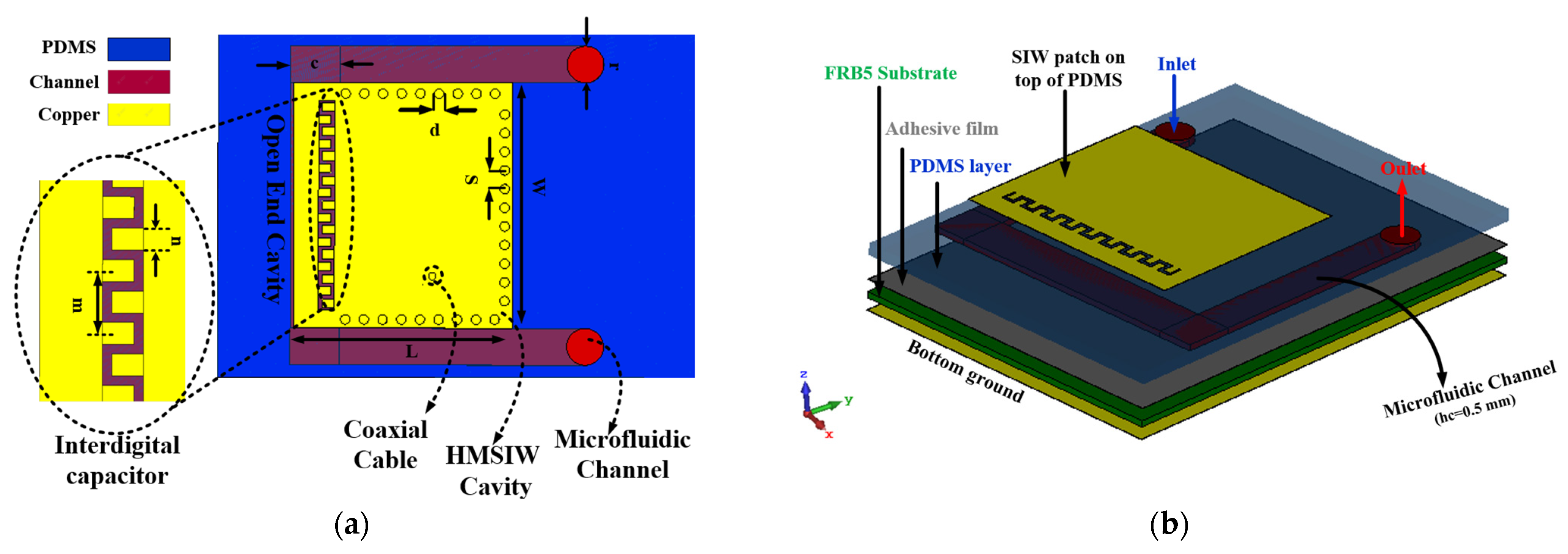
Figure 1. Configuration of the proposed HMSIW sensor: (a) top view, (b) layout view. Filling hole diameter r = 3 mm, channel width c = 5 mm, SIW diminutions (L = 17.7 mm, W = 20 mm), (vias diameter d = 0.77 mm, vias space S = 1.52), interdigital capacitor dimensions (n = 0.7 mm, m = 2 mm).
Energies 17 05208 g001
Figure 2. Top view of the proposed FMSIW cavity, (a) FMSIW, (b) HMSIW (REF1). The A–a and B–b lines mark the cutting edges of the magnetic walls.
Energies 17 05208 g002
Figure 3. Simulated electric field distributions of the fundamental mode TE101 at 6.2 GHz over (a) FMSIW cavity and (b) HMSIW cavity. The electric field distributions are minimal near the via walls (blue color) and strongly concentrated within the SIW cavity (red color).
Energies 17 05208 g003
Figure 4. Antenna structure evolution steps.
Energies 17 05208 g004
Figure 5. Fundamental equivalent circuit model of unit-section.
Energies 17 05208 g005
Figure 6. Simulated reflection coefficient of the REF 1 and REF 2 antennas, showing the electric field magnitude. The electric field distribution is represented using an intensity scale (heat map). The upper and lower rows indicate the minimum (blue) and maximum (red) magnitudes of the electric fields.
Energies 17 05208 g006
Figure 7. Simulated reflection coefficient of the loaded and unloaded antennas (REF 2 and REF 3).
Energies 17 05208 g007
Figure 8. Effective permittivity as a function of water temperature.
Energies 17 05208 g008
Figure 9. Simulated S11 of the sensor: (a) as a function of water temperature for different temperatures, (b) presence of ice, frost, and water.
Energies 17 05208 g009
Figure 10. The simulated far-field parameters of the HMSIW (unloaded): (a) total efficiency, (b) peak gain at 5.7 GHz.
Energies 17 05208 g010
Figure 11. Simulated far-field parameters of the antenna sensor for the sensing range: (a) total efficiency, (b) peak gain at 5.72 GHz.
Energies 17 05208 g011
Figure 12. Simulated normalized radiation patterns of sensor antenna at 5.72 GHz: (a) XY plane, (b) XZ plane.
Energies 17 05208 g012
Figure 13. The proposed ANN architecture. FC (resonance frequency), and the lower and upper frequencies (FL, Fu), hidden layers (HL), numbers of units (256, 128, 64, 16, etc.), and Early Frost (EF), Normal (N), and Early Wildfire (EW).
Energies 17 05208 g013
Figure 14. ANN Model accuracy for training and validation sets.
Energies 17 05208 g014
Table 1. Resonance frequency values at different water temperatures.
ε e f f F c , GHz T , °CState
87.744.91860Frost
86.54.92353Normal
84.14.92989Normal
78.64.942525Normal
71.74.959940High Temperature
67.74.972250High Temperature
3.25.69<0Ice
Table 2. Network hyper parameters.
LayersUnitsActivationKernel Initializer
1256ReLUglorot_normal
2128ReLUglorot_normal
364ReLUglorot_normal
416ReLUglorot_normal
58ReLUglorot_normal
63SoftMax-
Table 3. Validation samples with ML models.
LayersInputs, GHzML ModelsPredictedActual
f l f c f u
Sample 1
6 °C
4.92434.92434.9497ANNEFEF
RFEFEF
SVCEFEF
GPEFEF
Sample 2
8 °C
4.9274.9274.9522ANNNN
RFNN
SVCNN
GPNN
Sample 2
33.8 °C
4.964.964.99ANNEWEW
RFEWEW
SVCEWEW
GPEWEW
Table 4. Comparison between the proposed antenna and previous studies.
Ref.Antenna Mode/TypeMUTP#PUTDMMLApp
[21]Passive, MLSolid1permittivityNoHT
[22]Passive, MLSolid1permittivityNoHT
[23]Passive, MLSolid1permittivityNoHT
[24]Passive, MLSolid1permittivityNoHT
[25]Passive, MLSolid1permittivityNoHT
[26]Passive, MLSolid1permittivityNoHT
[27]Active, MLIce1ThicknessNoFrost
[*]MLLiquid3permittivityYesATR 1
# Numbers, * Proposed antenna, 1 All Temperature Range.
Disclaimer/Publisher’s Note: The statements, opinions and data contained in all publications are solely those of the individual author(s) and contributor(s) and not of MDPI and/or the editor(s). MDPI and/or the editor(s) disclaim responsibility for any injury to people or property resulting from any ideas, methods, instructions or products referred to in the content.