Article

A Generalized Deep Reinforcement Learning Model for Distribution Network Reconfiguration with Power Flow-Based Action-Space Sampling

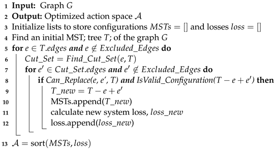
Electrical and Computer Engineering, University of Alberta, Edmonton, AB T6G 1H9, Canada
*
Author to whom correspondence should be addressed.
Energies 2024, 17(20), 5187; https://doi.org/10.3390/en17205187
Submission received: 21 September 2024 / Revised: 15 October 2024 / Accepted: 16 October 2024 / Published: 18 October 2024

Abstract

:
Distribution network reconfiguration (DNR) is used by utilities to enhance power system performance in various ways, such as reducing line losses. Conventional DNR algorithms rely on accurate values of network parameters and lack scalability and optimality. To tackle these issues, a new data-driven algorithm based on reinforcement learning is developed for DNR in this paper. The proposed algorithm comprises two main parts. The first part, named action-space sampling, aims at analyzing the network structure, finding all feasible reconfiguration actions, and reducing the size of the action space to only the most optimal actions. In the second part, deep Q-learning (DQN) and dueling DQN methods are used to train an agent to take the best switching actions according to the switch states and loads of the system. The results show that both DQN and dueling DQN are effective in reducing system losses through grid reconfiguration. The proposed methods have faster execution time compared to the conventional methods and are more scalable.

1. Introduction

The primary goal of distribution network reconfiguration (DNR) is to reduce power losses in the system by altering the network’s topology and switch settings [1]. DNR has become a fundamental part of distribution system operation due to power fluctuations caused by increasing penetration of distributed generation (DG) units and electric vehicles [2]. It can also increase the hosting capacity for distributed energy resources, improve the voltage profile, and minimize DG power curtailments.

1.1. Motivation and Literature Review

The DNR problem can be classified as a mixed-integer nonlinear problem that falls under the category of NP-hard problems, mathematically speaking [3]. The non-linearity of AC power flow and the radiality constraint of the network contribute to this classification. Therefore, it can only be optimized after simplifications [4] or through search algorithms [5]. To this end, the Lévy flight and chaos disturbed beetle antennae search (LDBAS) algorithm is used in [6] to solve a multi-objective dynamic reconfiguration model minimizing active power loss, load balancing index, and maximum node voltage deviation subject to stochastic power output from DG units and electric vehicles. Similarly, a multi-objective optimization problem is formulated in [7] and solved through a social beetle swarm algorithm to minimize network loss, load imbalance, and voltage deviation. In [8], the water cycle algorithm (WCA) is employed to address the network reconfiguration problem and to determine the optimal size and location of the DG units. Other relevant methods to solve network reconfiguration problem include the molecular differential evolution algorithm [9], Harris Hawks optimization (HHO) algorithm [10], Bayesian learning-based evolutionary algorithm [11], modified particle swarm optimization (PSO) [12], and genetic algorithm (GA) [13]. However, none of these methods can guarantee the optimality of the obtained solutions since they are only search algorithms. Furthermore, the time taken to execute them increases exponentially as the system size grows.
In the second type of study, mathematical programming and optimization methods are used to solve simplified formulations of the DNR problem. For instance, linear DistFlow equations are used in [14] to measure the voltage volatility of a bus and a Benders-decomposition-based method is used to solve the proposed DNR problem as a mixed-integer quadratic program (MIQP). Similarly, an MIQP model is proposed in [15] for the DNR problem after linearizing the power-flow equations. The DNR problem was addressed in [16] by formulating it as a mixed-integer linear model and solving it with the commercial solver CPLEX. This was achieved through the linearization of power-flow equations and load models. The major drawback of this approach is that, due to the linearization of power-flow equations and the use of simplified assumptions, the obtained results are not accurate.
Several recent studies have used machine learning techniques to perform the DNR procedure. The authors of [17] incorporated chaotic local search and quasi-oppositional-based learning techniques into the original neural network algorithm to tackle the challenges of network reconfiguration and distributed generation allocation concurrently. Nevertheless, optimization-focused artificial intelligence algorithms tend to have poor convergence and are highly susceptible to being trapped in local optima [6]. The authors of [18] used a long short-term memory (LSTM) network to capture the mapping mechanism present between load distribution and the most effective reconfiguration strategies. The study presented in [19] involved the training of a deep convolutional neural network to establish the correlation between the network structure and the short-term voltage stability performance by analyzing historical data. Once trained, the network was used for the DNR process. The primary drawback of these two techniques is that the size of the neural network required for training tends to increase as the network size grows, resulting in an increase in computational expenses. Moreover, as these networks are exclusively trained on past operational data, they cannot find novel reconfiguration strategies. The study in [20] employed a deep neural network to construct a probability distribution (PD) forecasting network that could anticipate the joint PD for DG outputs and loads. Subsequently, a variant of the column-and-constraint generation technique with efficient scenario decomposition solved the DNR problem in the worst-case scenario of PD for DG outputs and loads. In this instance, neural networks were only used to predict the PD of DG outputs.
Most current studies adopt a model-based control strategy for DNR, which requires exact knowledge of distribution network parameters. However, obtaining accurate parameter estimates is challenging for electric utilities due to the complex nature of distribution networks and changes caused by weather-related fluctuations [21]. Moreover, as the network size grows, the computational complexity of model-based algorithms rapidly increases, making real-time control infeasible [22].

1.2. Related Work

Reinforcement learning (RL) is a machine learning technique based on the action and response process; it has been successful in solving many difficult sequential decision-making problems [23]. In the process of transforming DNR into a Markov decision process (MDP) for RL, each instance of manipulating various switches to either open or closed is regarded as a singular action. As a consequence, the action space becomes notably expansive. Therefore, the primary challenge when using RL for DNR lies in effectively managing this extensive action space while also ensuring the optimality of the achieved outcomes compared to alternative mathematical or heuristic methods.
In terms of addressing this challenge, RL studies can be divided into three groups. In the first set of studies, the RL agent is trained on only a very limited historical operational dataset. To this end, the method proposed in [24] for DNR involves training a batch-constrained soft actor–critic RL algorithm using a finite historical operational dataset. However, the performance of this algorithm largely depends on accurate historical DNR data, which is difficult to obtain. In addition, the algorithm does not search for new reconfiguration strategies since it is trained only on previous strategies that might not be optimal.
The second set of studies utilize the multi-agent RL approach to manage the extensive action space. This is achieved by distributing the action space among multiple agents. In [25], a complex multi-objective DNR model is introduced, considering multiple factors, including renewable energy curtailment, voltage stability, power loss, and generation cost. It is solved using a deep Q-learning (DQN)-assisted multi-objective bacterial foraging optimization algorithm. To reduce the action-space size, the action space is divided into smaller subspaces, with each subspace being handled by a separate DQN. The study in [26] introduces a deep RL-based method to reconfigure distribution networks during extreme events, creating microgrids to restore critical services. The approach employs a multi-agent soft actor–critic (MA-SAC) strategy to efficiently control circuit breakers for isolating sections of the network and accommodating various system states and scales. In [27], a cloud–edge collaboration architecture is developed and combined with a deep RL model for real-time optimal reconfiguration of urban distribution networks. This approach involves multi-level dynamic reconfiguration, integrating feeder, transformer, and substation levels, using a multi-agent system. The model employs both offline and online learning phases, incorporating a Q-learning-based multi-agent conservative Q-learning algorithm for stability in offline learning, and a multi-agent deep deterministic policy gradient algorithm for exploration and experience pool updates in online learning. The primary limitation of this methodology stems from the extensive action space within large systems, such as the 136-node test system encompassing over three million feasible actions. Consequently, even after partitioning this action space among multiple agents, its sheer magnitude persists, presenting a challenge for comprehensive action-space exploration. Furthermore, all of these studies lack direct comparisons with solutions documented in the existing literature; thus, the efficacy of the proposed approach remains uncertain.
The third category of studies does not present any approach for reducing the dimensions of the action space. In such cases, it is not clear how the action space for the DNR agent is selected. These studies include a branching double DQN (BDDQN) and multi-policy soft actor–critic (MPSAC) for rapid decision making in sequential reconfiguration with soft open points in [28], a DQN method to address DNR within both the IEEE 33-node system and a real-life, large-scale testing environment in [29], a DQN-based network reconfiguration to enhance the reliability of distribution networks, particularly when confronted with the fluctuating nature of distributed renewable energy resources in [30,31], and a NoisyNet DQN method coupled with a loop-based encoding for DNR in [32]. Finally, a dynamic network reconfiguration strategy aimed at minimizing operation costs and load shedding is introduced in [33]. It employs a three-stage deep RL approach to optimize the reconfiguration and set-points of distributed generators in real-time, enhancing distribution network stability and reliability by quickly adapting to events and uncertainties. Double DQN (DDQN) is used in the offline learning process for optimal reconfiguration and three RL algorithms including deep deterministic policy gradient (DDPG), soft actor–critic, and twin-delayed DDPG (TD3) are evaluated to determine the real-time set-points of distributed generators and energy storage systems. However, this study does not describe any method to reduce the dimension of the action space.

1.3. Contributions

Managing the extensive action space within the DNR problem is a crucial topic in ensuring the optimality and faster convergence of RL algorithms, and it has not been adequately addressed in previous research. To address the limitations encountered in the existing literature regarding the effective management of extensive action spaces within the DNR problem, this paper introduces an innovative approach for reducing the dimensions of action space. This method leverages a graph theory-based procedure, known as the Yamada–Kataoka–Watanabe algorithm, in conjunction with power-flow analysis. Employing the DQN and dueling DQN methodologies, this approach trains agents to select optimal switching actions across a range of distribution systems, substantially improving the convergence and optimality of the solutions obtained by the RL agent. A comprehensive comparative analysis is conducted between these two advanced techniques and the conventional methodologies in the literature. Through this comparison, the respective merits and drawbacks, as well as the optimality of the obtained solutions are demonstrated. The following are the key contributions of this paper:
  • Development of a novel method rooted in graph theory and power-flow analysis, aimed at reducing the size of the action space, which enhances the optimality and convergence of solutions generated by RL algorithms;
  • Conducting a comprehensive sensitivity analysis of the action-space dimensions to demonstrate the substantial impact of action-space size on the performance of the RL agent;
  • A thorough comparative analysis between the proposed method and conventional DNR methods in terms of execution speed and optimality of the obtained solutions, confirming the effectiveness of the proposed method.
The remainder of the paper is organized as follows. Section 2 covers key RL preliminaries and provides an overview of relevant RL algorithms. Section 3 explains the formulation of the problem as an RL task and introduces the proposed method for action-space sampling. In Section 4, the main results, applying the method to 33-, 119-, and 136-node test systems, along with a sensitivity analysis and a comparison with previous studies, are presented. Finally, Section 5 provides the concluding remarks.

2. RL Foundations and Algorithms

This section focuses on the fundamental principles and key algorithms that form the basis of RL. It lays the groundwork by explaining the core concepts of RL, including the agent–environment interaction, states, actions, rewards, and the objective of learning optimal strategies. The section further explores various RL algorithms, providing insights into their workings, advantages, and applications.

2.1. RL Preliminaries

In a standard RL structure, an agent interacts with an environment E for a number of steps and receives an instant reward r t + 1 for each action a t that it performs inside E at time step t. After performing the action a t at time t according to state s t , the environment arrives at a new state s t + 1 . The process is illustrated in Figure 1. The aim of the agent is to increase its cumulative reward over time. To use RL, it is necessary to create an environment that can be modeled as an MDP. This involves defining the action space A , state space S , reward function R , transition probabilities P , discount factor γ , and time horizon T .
Based on the present state s t S , the agent chooses an action a t A . After the agent executes the selected action in the environment, it receives a reward r t + 1 , determined by the current state s t and the action taken a t . Subsequently, the agent transitions to a new state, determined by the state transition probability function P . The control process can either continue indefinitely with T , or it can end when the time step t reaches the final time T . Finally, the agent determines the optimal control policy π that maximizes the expected discounted return G computed by taking the sum of the rewards obtained at each time step in episodic tasks and as G t = j = 0 γ j r t + j + 1 in continuous tasks. The Bellman optimality equation is used in each state to find the optimal action value function, denoted by Q π ( s t , a t ) . In each state, the optimal policy is the one that maximizes the rewards, hence π * = argmax a Q * ( s , a ) . However, at the beginning of the training, the optimal Q-values are unknown. In deep RL algorithms, the q-values are determined using a target neural network ( Q _ t a r g ) and the Bellman equation. Therefore, the policy neural network is updated by minimizing the following temporal difference error:
δ = Q π ( s t , a t ) ( r ( s t , a t ) + γ max a Q _ t a r g ( s t + 1 , a ) ) .

2.2. RL Algorithms

The behavior policy refers to the policy adopted by the agent to make its action choices, while the target policy is the one that the agent aims to acquire through learning. In general, there are two types of RL algorithms: on-policy and off-policy. On-policy learning refers to a method where the behavior and target policies used by the agent are the same, whereas in off-policy learning, they are distinct. As a result, on-policy learning has a higher chance of becoming stuck in a suboptimal policy. Therefore, in this DNR study, two off-policy methods are implemented and tested: DQN and dueling DQN.
In DQN, the policy is determined by a neural network. The input of this neural network is the state of the agent and the output is the Q-value for each action in the action space. DQN overcomes unstable learning by using experience replay and target network. Using experience replay, previous transitions are stored in memory as ( s t , a t , r t + 1 , s t + 1 ). Later, these transitions are sampled from the memory in mini-batches and used to update the neural network. In this way, the correlation between experiences to update the neural network is reduced and catastrophic forgetting is prevented by reusing past transitions. Catastrophic forgetting or policy collapse is a common issue in policy gradient methods, where the agent starts to forget a policy it has learned before.
Algorithm 1 briefly describes the general training process of RL algorithms. For a specified number of steps, an action is chosen by the policy and executed to obtain a full trajectory ( s t , a t , r t + 1 , s t + 1 ) (lines 3–5). The transitions are added to the memory and a batch of transitions are chosen from the memory to compute the loss and update the policy (lines 6–8).
Algorithm 1: RL Training Procedure
Energies 17 05187 i001
Dueling DQN is an improved version of DQN. In some states, performing an action does not always increase the obtained reward. Therefore, in this method, it is unnecessary to know the value of each action at every time step instead, the state value and advantage function are used to find the optimal policy. The state value is the expected sum of discounted returns when starting from that state and is expressed as
V π ( s ) = E π [ t = 0 T 1 γ t r t | s t = s ] .
The difference between the action value and the state value is computed to obtain the advantage function, which can be expressed as
A π ( s , a ) = Q π ( s , a ) V π ( s ) .
The advantage function is utilized to determine the relative benefit of choosing an action compared to other actions at a particular state. In the dueling DQN method, one neural network with two streams is used to compute both the state value and advantage function. Then, the Q-value for the policy network is calculated according to
Q π ( s t , a t ) = V ( s t ) + ( A π ( s t , a t ) 1 | A π | a A π ( s t , a ) ) .
Similarly to the DQN method, a target neural network (which is a copy of the policy neural network) is used to calculate the values of V _ t a r g ( s t + 1 ) , A _ t a r g ( s t + 1 , a t + 1 ) , and eventually, Q _ t a r g ( s t , a ) . The policy network is iteratively updated using the temporal difference error from Equation (1).

3. Problem Formulation

In this section, the basics of RL are first discussed. Then, the DNR problem is reformulated as an MDP. Finally, the power flow-based action-space sampling method is proposed and two RL algorithms for training the agents are presented.

3.1. System Modeling

In reconstructing the DNR as an MDP problem, the opening and closing of each line is considered an action. The system receives the action in binary format, where a zero value shows an open line and one shows a closed line. In this study, an agent can open or close as many lines as needed in a single action. For example, changing the line states from [1, 1, 1, 0, 1, 0] to [1, 1, 1, 1, 0, 1] is considered one action. This form of representation allows avoiding loops or disconnections in the system while opening or closing lines. The state of the system, shown as s t = [ p t , q t , α t ], is the real ( p t = [ p 1 t , p 2 t , , p n t ] ) and reactive ( q t = [ q 1 t , q 2 t , , q n t ] ) power consumption of the buses as well as the switch states, α t = [ α 1 t , α 2 t , , α m t ] . Parameters n and m denote the number of buses and lines in the system, respectively. After each action, the time t is incremented by 1. The random process of power injections is assumed to represent the transition probability, P , between time steps.
Since the aim of DNR in this paper is to minimize the total line losses, the reward function is defined as
R ( s t , a t ) = C p l t ( s t + 1 ) R _ v ( s t + 1 ) .
In this equation, the penalty function for line losses, in 1/kW, is represented by C, and p l t ( s t + 1 ) denotes the total line losses at state s t + 1 . The second term is defined as the penalty function R _ v ( s t + 1 ) for violating the voltage constraint of the system and is computed as   
R _ v ( s t + 1 ) = λ ( max ( V t , n ) 1 ) if V max < max ( V t , n ) λ ( 1 min ( V t , n ) ) if min ( V t , n ) < V min 0 otherwise .
Here, a significantly high value is assigned to the variable λ to represent a highly negative reward when an action causes voltage violation in the system. The variable V t , n represents voltage at time t at bus n and V max and V min denote the maximum and minimum voltage limits in the system. Other system constraints, including radiality and load balance constraints, are imposed while selecting the action space A , as described in the following subsection.

3.2. Action-Space Sampling

The original action space for DNR is extremely vast. If there are 33 lines in the system and all lines have switches to be opened and closed, the complete action space contains 233 actions. However, the majority of these actions are not practical to be executed in an actual distribution system because they can cause loops or disconnections in the network. Therefore, a graph theory-based algorithm named Yamada–Kataoka–Watanabe [34] is used in this study to form the action space for RL by only selecting the feasible actions. The Yamada–Kataoka–Watanabe algorithm can identify every minimum spanning tree present in an undirected graph. All power networks can be considered undirected graphs where each bus is a node and the power lines are edges. A minimum spanning tree refers to a selection of edges from a graph, which connects all nodes without forming any cycles. Therefore, using this algorithm, a set of all reconfigurations and actions that cause no disconnections and loops in the power system can be found. This set is called the feasible action space.
The feasible action space for power networks can still be fairly large. Therefore, a rational action-space sampling method is needed to only select the optimal actions as the final action space. For instance, consider the schematic diagram of an IEEE 33-node distribution system [35] with a total demand of 22,709 MW and 17,041 MVAr depicted in Figure 2. Although opening the lines 2–19, 9–10, 15–14, 25–29, 32–22, and closing the lines 7–8 and the rest of the lines is a feasible reconfiguration action, it cannot be considered an optimal action since it would open a line very close to the substation and would put too much load on other lines, increasing the system loss.
To address this issue, a new power flow-based action-space sampling method is developed in this paper to only select the optimal actions as the DNR action space. At the same time, this reduces the action-space size and further improves the convergence of the RL algorithm. In this method, a power flow is performed first, considering the standard load values and assuming that all lines are closed. Then, active power losses of each line are calculated. This is shown by red numbers in Figure 2. Finally, the total system losses for each of the feasible actions are calculated and the actions are sorted based on the system loss. The optimal actions are the ones with higher calculated system loss. This is because, according to Figure 2, lines near the main substation carry more current and have more active power losses. Therefore, disconnecting these lines causes more reduction in overall system losses. As a result, the actions with higher calculated losses disconnect lines further away from the substation and are optimal.
To adapt the Yamada–Kataoka–Watanabe method together with power flow-based action-space sampling to the DNR problem, a graphical model of the power system network as an undirected graph G = ( V , E ) is first developed, where each node v V corresponds to a bus, and each edge e E represents a distribution line. Later, Algorithm 2 is employed to identify feasible actions and rank them according to their effectiveness.
Algorithm 2: Graph of Power-Flow Action Sampling
Energies 17 05187 i002

4. Simulation and Results

To verify the effectiveness of the proposed method, it is applied to solve DNR in 33-, 119-, and 136-node test systems. Section 4.1 presents the parameters of the algorithms used for the simulations. Section 4.2 presents the results of the action-space sampling. Section 4.3, Section 4.4 and Section 4.5 describe the results obtained by applying the proposed method on test systems. A sensitivity analysis is discussed in Section 4.6. Finally, the proposed method is compared with other studies in Section 4.7.

4.1. Experimental Setup and Data

The lower and upper limits for the voltage levels in constraint (6) are defined as 0.95 p.u. and 1.05 p.u., respectively. Based on empirical performance, the value of the parameter R l is assigned as 10,000 and λ as 1,000,000. The pandapower package in Python is used to create a model of the power network, and the Newton–Raphson method to perform power-flow calculations. The graph analysis is performed using the NetworkX package (version 3.1) and the Yamada–Kataoka–Watanabe algorithm. Hourly load data for 3000 days are generated by assuming a normal distribution with a standard deviation of 15% to the standard 33-, 119-, and 136-bus network loads. The input states, comprising the active and reactive power of the buses’ and switches’ states, are scaled using min–max scaling to ensure that they contribute equally to the learning process. The tuned parameters of the DQN and dueling DQN algorithms are given in Table 1.

4.2. Action-Space Sampling

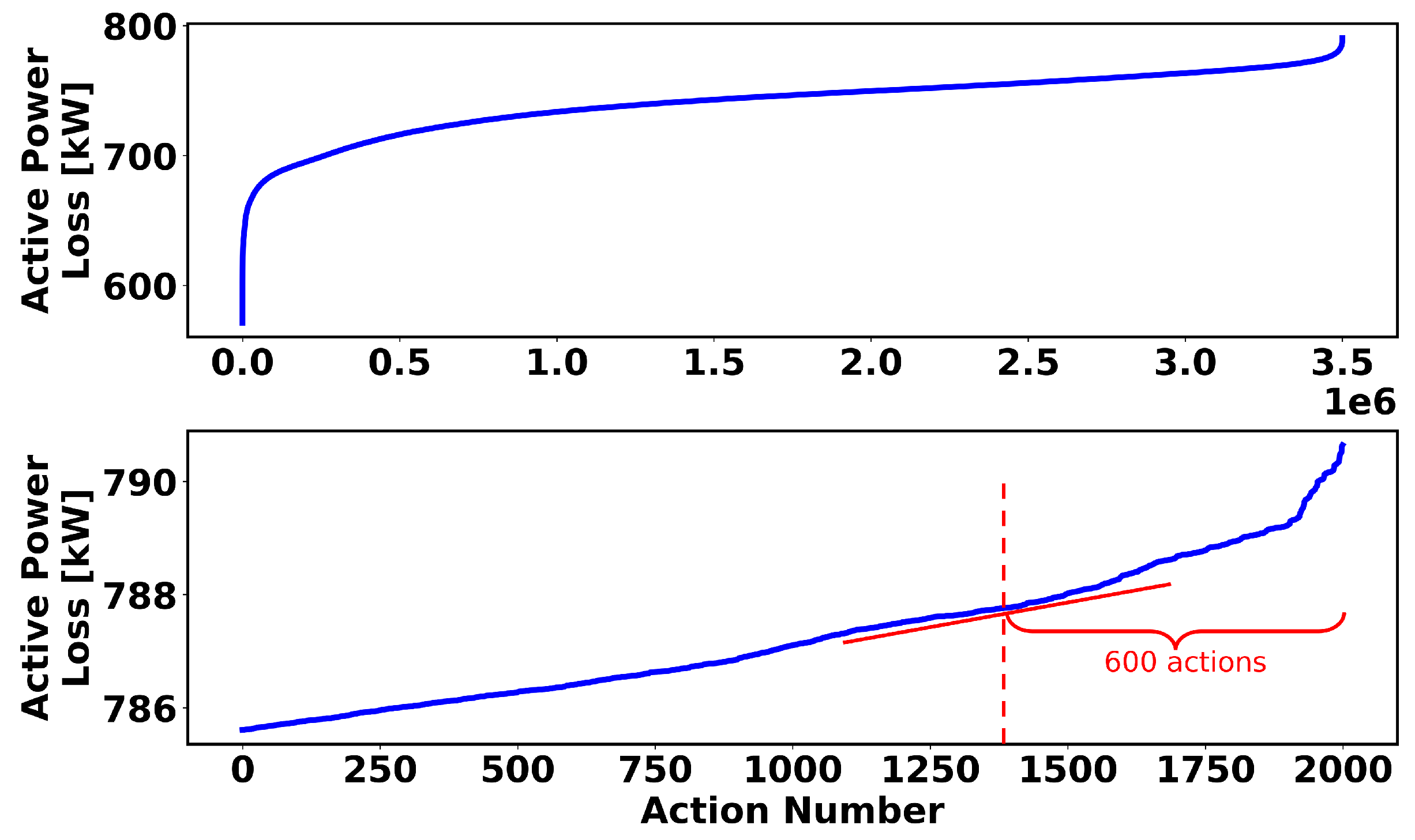
When applying the Yamada–Kataoka–Watanabe algorithm to the 33-node test system, 50,751 feasible actions are found. Applying the same algorithm to the 119- and 136-node test systems finds more than 3,500,000 feasible actions. However, to prevent the memory overflow problem, the number of feasible actions is restricted to 3,500,000. Using the proposed action-space sampling methodology, the sorted values of losses for the 33-node system are depicted in Figure 3. The top illustration presents the sorted active power loss for all the feasible actions in the 33-node system. On the other hand, the lower illustration presents an enlarged perspective of the aforementioned upper illustration, focusing on a subset of 2000 actions from the right side. Since the active power reduction slope decreases after 300 actions, the top 300 actions are chosen as the optimal actions for the 33-node system.
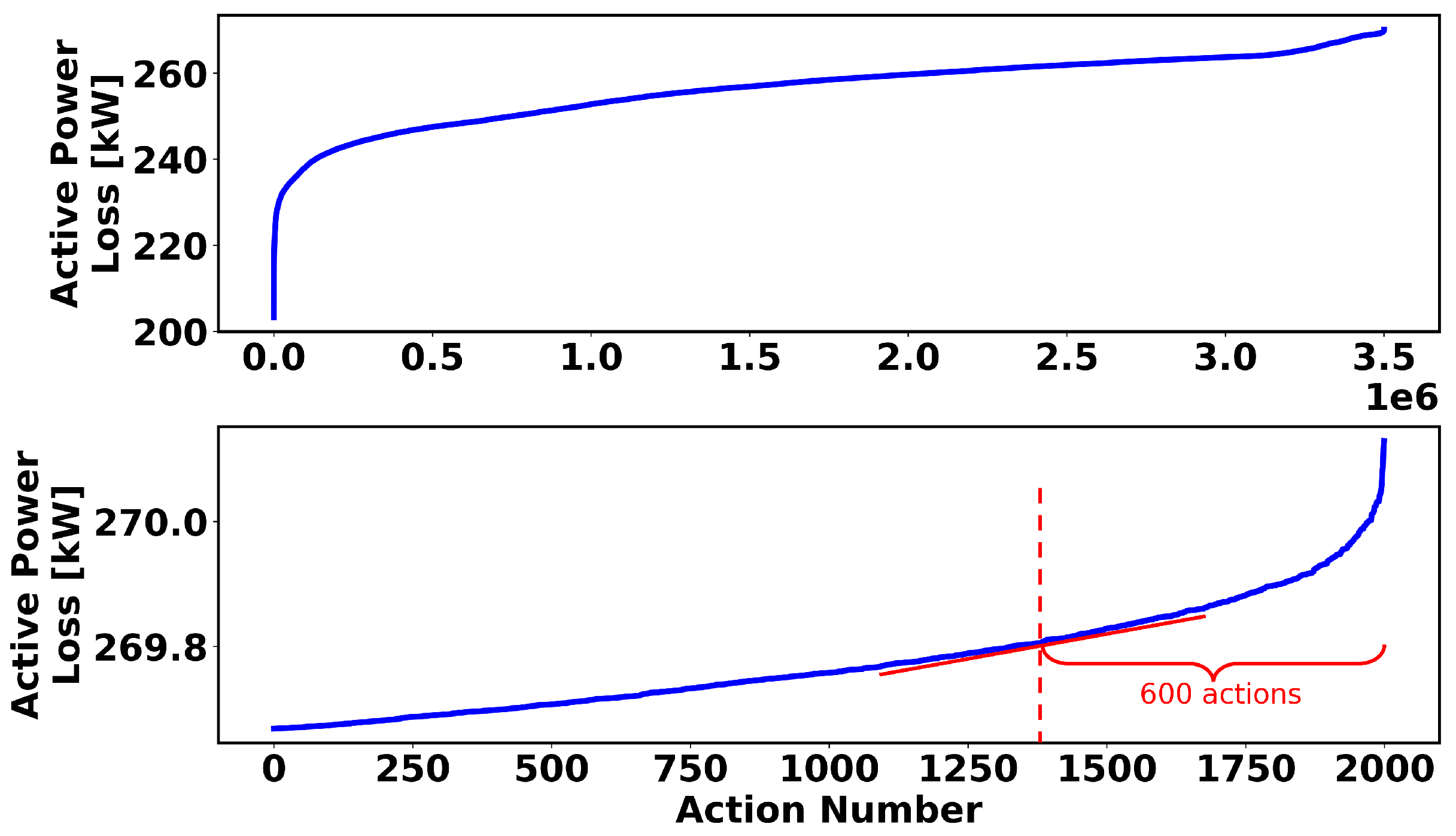
The sorted values of active power losses for different actions in the 119- and 136-node test systems are illustrated in Figure 4 and Figure 5, respectively. Similarly, the top 600 actions are selected as the optimal actions to form the action space for the RL algorithms in the 119- and 136-node systems, as this provides a trade-off between loss reduction and the action-space size. It is important to note that a comprehensive sensitivity analysis on the action-space size is conducted in Section 4.6.
This study makes a significant contribution by introducing a new action-space sampling method, which greatly improves the efficacy of RL agents in achieving optimal solutions. Additionally, by careful hyperparameter tuning, factors such as the balance between exploration and exploitation, neural network size for function approximation, and learning rate are adjusted to ensure optimal rewards and solutions. In essence, ensuring the accuracy of DQN and dueling DQN involves a holistic approach that encompasses comprehension of their theoretical foundations, thorough analysis of components like function approximation and experience replay, strategic hyperparameter optimization, and rigorous empirical assessments to validate their performance across diverse tasks.

4.3. The 33-Node Test System

The IEEE 33-node test system is a very popular network for power system studies. This network is operated at 12.66 kV and has a total demand of 22,709 MW and 17,041 MVAr. Given the persistent interaction of the RL agent with the environment spanning over 50,000 iterations, the obtained rewards tend to exhibit fluctuations when directly visualized. Therefore, a good strategy for assessing the progression of reward accumulation is to calculate the mean value of daily rewards. Additionally, to effectively represent the upward trend in these rewards, it is conventional in the field of RL to employ a technique known as the “n-step moving average” of rewards. Applying these techniques to the 33-node system, Figure 6 shows the average daily rewards and the 60-step moving average for the DQN and dueling DQN algorithms as they train and converge. When the obtained rewards stabilize, it is an indication of convergence of the RL algorithm and the training can be stopped. In the visualized figures, the higher the obtained rewards, the better the algorithm has performed. It appears from these figures that the RL agent can find a control policy that minimizes system losses. Therefore, the obtained rewards increase over time. In addition, DQN converges faster than dueling DQN.
The small fluctuations after convergence are mainly due to load fluctuations at different hours and the exploration property of the algorithms. Table 2 presents the DNR solution obtained using DQN and dueling DQN in the 33-node system for a single hour. The tie switches represent the open lines.

4.4. The 119-Node Test System

To demonstrate the scalability of the proposed method, it is applied to a large-scale 119-node test system [36]. The nominal voltage of this network is 11 kV, and the total demand is 22,709 MW and 17,041 MVAr. The average daily rewards using DQN and the 60-step moving average are depicted in Figure 7. These curves show that the agent learns to choose better actions and maximize rewards over time. Also, the convergence time is acceptable.
The DNR result for a single hour is given in Table 3. Overall, the results show that the proposed method performs well for a large-scale distribution system and that the convergence time is at an acceptable level.

4.5. The 136-Node Test System

To demonstrate the applicability of the proposed method on a real test system, it is tested on a 136-node system in the Midwest of Brazil [37]. This network has a relatively complex structure and operates at 13.8 kV. Figure 8 shows the average daily rewards and the moving average during training in the 136-node test system. Similar to the other test cases, the rewards increase over time, indicating agent learning, and DQN converges faster than dueling DQN. DNR results for a single operating hour are given in Table 4.

4.6. Sensitivity Analysis

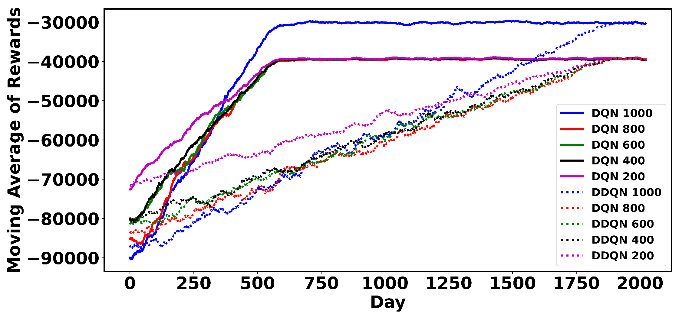
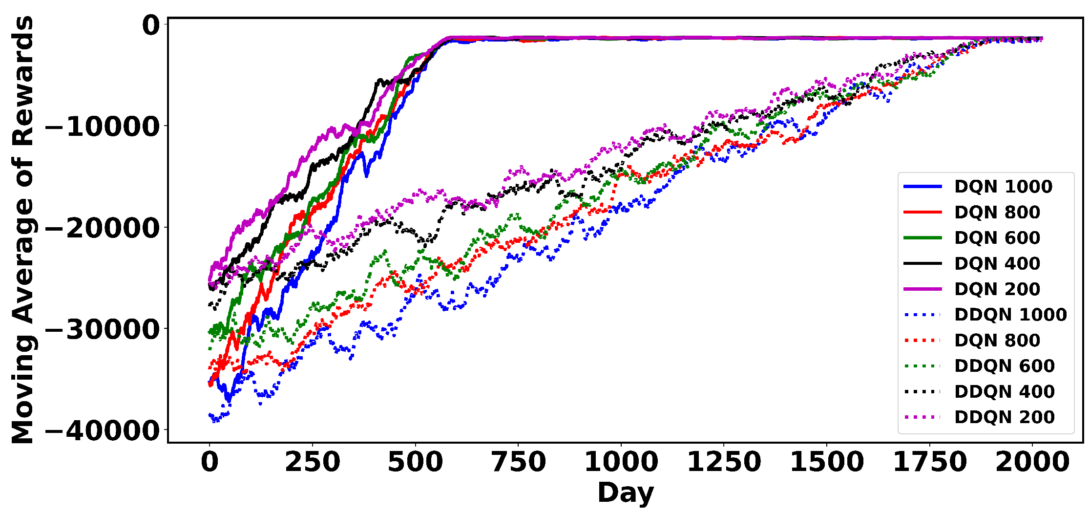
To investigate the effect of selecting a different number of actions on the results, simulations are repeated with various sizes of action sets. The results are presented in Figure 9, Figure 10 and Figure 11. It can be observed from Figure 9 that increasing the action-space size from 200 to 500 does not have much impact on the rewards obtained in the 33-node system. However, choosing a much smaller action space (e.g., 100) significantly reduces the obtained rewards. Therefore, it can be concluded that the optimal actions are within the first batch of 200 actions.
In the 119-node test system, action-space sizes of 200, 400, 600, and 800 obtain similar rewards. However, increasing the size to 1000 significantly improves the obtained rewards. This indicates that the optimal actions lie within the initial batch of 1000 actions. In the 136-node system, action-space sizes of 200–1000 all obtain similar rewards since the best actions are within the first batch of 200 actions.
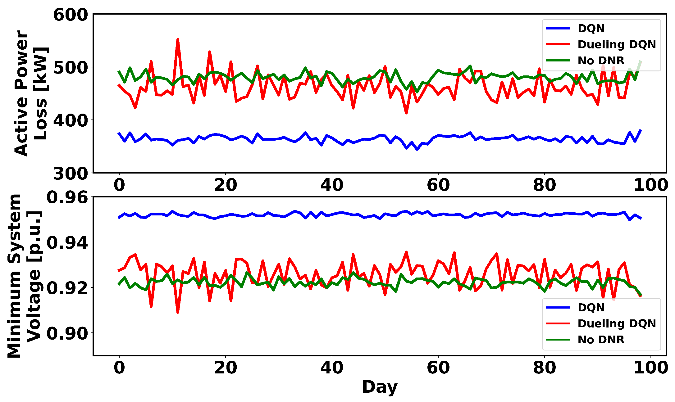
To show the robustness of the proposed method under extreme load fluctuation events, the load values are intentionally changed to significantly deviate from the average load on which the RL algorithms were trained. For this purpose, the standard deviation of these loads is set at 35% of the previous average loads. The trained RL algorithms are executed for 2400 steps and the results are averaged daily. The system loss and minimum system voltage in this case are shown in Figure 12, Figure 13 and Figure 14 for the 33-, 119- and 136-node systems, respectively. Comparing the obtained results with the base case where there is no DNR in the system reveals that, using DQN and dueling DQN, the loss is lower and the voltage is higher, and the agent chooses the actions that minimize the system loss and improve the voltage profile. In the 119- and 136-node test systems, the dueling DQN sometimes chooses actions that are not optimal. Therefore, it can be concluded that DQN is more robust to unforeseen states or extreme events.
In RL studies, the reward function is typically designed to optimize the agent’s performance. This study performs a sensitivity analysis on the reward function coefficient to validate that its parameters indeed enhance performance. Voltage limit violations render the power network inoperable, necessitating avoiding such scenarios. By assigning a high value to the parameter λ , the agent can effectively avoid such conditions. Consequently, this analysis focuses on the impact of varying C. Figure 15 illustrates the system loss and voltage penalty associated with different C values. It is evident that while the voltage penalty remains consistent across various C values, setting C to 10,000 leads to a significantly lower system loss.

4.7. Comparative Study

In this section, the computational speed of the proposed method and the optimality of its results are compared with published results obtained using the switch opening and exchange (SOE) [35] mathematical programming (MP) methods (which encompass mixed-integer linear and mixed-integer nonlinear programming) [35], adaptive ant colony optimization (AACO) method [5], MIQP [15], and two RL methods, BCSAC [24] and NoisyNet DQN [32]. The DNR execution times of all these methods are given in Table 5. As can be inferred from this table, the execution times for DQN and dueling DQN are quite similar, and both are significantly faster compared to other non-RL methods in the 136-node system, with a speed improvement factor of at least twenty. The efficiency of the RL algorithms becomes even more important as the system size increases. The offline training times for DQN and dueling DQN algorithms are given in the last row of the same table. Training was carried out on a system with an Intel i9-9820X 3.30 GHz CPU and 100 GB of RAM.
Finally, the optimality of the results obtained by the proposed method is compared with other published results in Table 6. As can be seen, the results for the small 33-node system are within only a 0.3% optimality gap of the best solution presented in the literature and the maximum optimality gap that occurs for the 119-node system is only 10.58%. In heuristic methodologies, adherence to system constraints is ensured by imposing large penalties when they are violated. As a consequence, these methods occasionally find solutions that effectively minimize the objective function; nonetheless, their feasibility may be compromised. Such challenges are often encountered in solutions documented in the existing literature. Conversely, the results obtained by the approach proposed in this study do not exhibit any constraint violations.

5. Conclusions

This article employed a Markov decision process as a modeling technique for the DNR problem and leveraged two RL algorithms, namely, DQN and dueling DQN, to tackle the problem. First, the feasible action space for DNR was obtained using the Yamada–Kataoka–Watanabe algorithm. Then, a power flow-based action sampling method was applied to reduce the size of the action space. This was to facilitate faster convergence of the RL algorithms and optimize the results. The proposed method was applied to 33-, 119-, and 136-node test systems to demonstrate its scalability.
The results indicated that the learning performances of DQN and dueling DQN are very similar. However, DQN has faster convergence. In addition, a comparison with conventional methods proved that the proposed RL-based method is at least 20-times faster and that the obtained results are within a maximum 10.58% optimality gap of the best solution presented in the literature. This demonstrated that the proposed power flow-based action-space sampling method was effective and it only chose the most optimal actions. Future studies will focus on implementing the same method for semi-open lines to increase the electric vehicle hosting capacity and balance network loads.

Supplementary Materials

The following supporting information can be downloaded at: https://www.mdpi.com/article/10.3390/en17205187/s1.

Author Contributions

Conceptualization, P.M.; methodology, N.G.; investigation, N.G.; resources, P.M.; writing—original draft preparation, N.G.; writing—review and editing, P.M.; supervision, P.M.; project administration, P.M.; and funding acquisition, P.M. All authors have read and agreed to the published version of the manuscript.

Funding

This research was funded by the Natural Sciences and Engineering Research Council (NSERC) of Canada grant number ALLRP 549804-19 and by Alberta Electric System Operator, AltaLink, ATCO Electric, ENMAX, EPCOR Inc., and FortisAlberta.

Data Availability Statement

Data available on request due to restrictions (large data size). A minimal data representing the original has been provided at submission and is available in Supplementary Material.

Conflicts of Interest

The authors declare that this study received funding from Alberta Electric System Operator, AltaLink, ATCO Electric, ENMAX, EPCOR Inc., and FortisAlberta. The funder was not involved in the study design, collection, analysis, interpretation of data, the writing of this article or the decision to submit it for publication.

References

  1. Pereira, E.C.; Barbosa, C.H.N.R.; Vasconcelos, J.A. Distribution Network Reconfiguration Using Iterative Branch Exchange and Clustering Technique. Energies 2023, 16, 2395. [Google Scholar] [CrossRef]
  2. Mahdavi, E.; Asadpour, S.; Macedo, L.H.; Romero, R. Reconfiguration of Distribution Networks with Simultaneous Allocation of Distributed Generation Using the Whale Optimization Algorithm. Energies 2023, 16, 4560. [Google Scholar] [CrossRef]
  3. Gao, H.; Ma, W.; Xiang, Y.; Tang, Z.; Xu, X.; Pan, H.; Zhang, F.; Liu, J. Multi-objective Dynamic Reconfiguration for Urban Distribution Network Considering Multi-level Switching Modes. J. Mod. Power Syst. Clean Energy 2022, 10, 1241–1255. [Google Scholar] [CrossRef]
  4. Hong, H.; Hu, Z.; Guo, R.; Ma, J.; Tian, J. Directed graph-based distribution network reconfiguration for operation mode adjustment and service restoration considering distributed generation. J. Mod. Power Syst. Clean Energy 2017, 5, 142–149. [Google Scholar] [CrossRef]
  5. Swarnkar, A.; Gupta, N.; Niazi, K. Adapted ant colony optimization for efficient reconfiguration of balanced and unbalanced distribution systems for loss minimization. Swarm Evol. Comput. 2011, 1, 129–137. [Google Scholar] [CrossRef]
  6. Wang, J.; Wang, W.; Wang, H.; Zuo, H. Dynamic Reconfiguration of Multiobjective Distribution Networks Considering DG and EVs Based on a Novel LDBAS Algorithm. IEEE Access 2020, 8, 216873–216893. [Google Scholar] [CrossRef]
  7. Chen, Q.; Wang, W.; Wang, H.; Wu, J.; Li, X.; Lan, J. A Social Beetle Swarm Algorithm Based on Grey Target Decision-Making for a Multiobjective Distribution Network Reconfiguration Considering Partition of Time Intervals. IEEE Access 2020, 8, 204987–205013. [Google Scholar] [CrossRef]
  8. Muhammad, M.A.; Mokhlis, H.; Naidu, K.; Amin, A.; Franco, J.F.; Othman, M. Distribution Network Planning Enhancement via Network Reconfiguration and DG Integration Using Dataset Approach and Water Cycle Algorithm. J. Mod. Power Syst. Clean Energy 2020, 8, 86–93. [Google Scholar] [CrossRef]
  9. Peng, C.; Xu, L.; Gong, X.; Sun, H.; Pan, L. Molecular Evolution Based Dynamic Reconfiguration of Distribution Networks With DGs Considering Three-Phase Balance and Switching Times. IEEE Trans. Ind. Inform. 2019, 15, 1866–1876. [Google Scholar] [CrossRef]
  10. Helmi, A.M.; Carli, R.; Dotoli, M.; Ramadan, H.S. Efficient and Sustainable Reconfiguration of Distribution Networks via Metaheuristic Optimization. IEEE Trans. Autom. Sci. Eng. 2022, 19, 82–98. [Google Scholar] [CrossRef]
  11. Zhong, T.; Zhang, H.T.; Li, Y.; Liu, L.; Lu, R. Bayesian Learning-Based Multi-Objective Distribution Power Network Reconfiguration. IEEE Trans. Smart Grid 2021, 12, 1174–1184. [Google Scholar] [CrossRef]
  12. Fu, Y.Y.; Chiang, H.D. Toward Optimal Multiperiod Network Reconfiguration for Increasing the Hosting Capacity of Distribution Networks. IEEE Trans. Power Deliv. 2018, 33, 2294–2304. [Google Scholar] [CrossRef]
  13. Cebrian, J.C.; Kagan, N. Reconfiguration of distribution networks to minimize loss and disruption costs using genetic algorithms. Electr. Power Syst. Res. 2010, 80, 53–62. [Google Scholar] [CrossRef]
  14. Song, Y.; Zheng, Y.; Liu, T.; Lei, S.; Hill, D.J. A New Formulation of Distribution Network Reconfiguration for Reducing the Voltage Volatility Induced by Distributed Generation. IEEE Trans. Power Syst. 2020, 35, 496–507. [Google Scholar] [CrossRef]
  15. Ahmadi, H.; Martí, J.R. Distribution System Optimization Based on a Linear Power-Flow Formulation. IEEE Trans. Power Deliv. 2015, 30, 25–33. [Google Scholar] [CrossRef]
  16. Franco, J.F.; Rider, M.J.; Lavorato, M.; Romero, R. A mixed-integer LP model for the reconfiguration of radial electric distribution systems considering distributed generation. Electr. Power Syst. Res. 2013, 97, 51–60. [Google Scholar] [CrossRef]
  17. Tran, T.V.; Truong, B.H.; Nguyen, T.P.; Nguyen, T.A.; Duong, T.L.; Vo, D.N. Reconfiguration of Distribution Networks With Distributed Generations Using an Improved Neural Network Algorithm. IEEE Access 2021, 9, 165618–165647. [Google Scholar] [CrossRef]
  18. Liu, N.; Li, C.; Chen, L.; Wang, J. Hybrid Data-Driven and Model-Based Distribution Network Reconfiguration With Lossless Model Reduction. IEEE Trans. Ind. Inform. 2022, 18, 2943–2954. [Google Scholar] [CrossRef]
  19. Huang, W.; Zheng, W.; Hill, D.J. Distribution Network Reconfiguration for Short-Term Voltage Stability Enhancement: An Efficient Deep Learning Approach. IEEE Trans. Smart Grid 2021, 12, 5385–5395. [Google Scholar] [CrossRef]
  20. Zheng, W.; Huang, W.; Hill, D.J.; Hou, Y. An Adaptive Distributionally Robust Model for Three-Phase Distribution Network Reconfiguration. IEEE Trans. Smart Grid 2021, 12, 1224–1237. [Google Scholar] [CrossRef]
  21. Gao, Y.; Foggo, B.; Yu, N. A Physically Inspired Data-Driven Model for Electricity Theft Detection With Smart Meter Data. IEEE Trans. Ind. Inform. 2019, 15, 5076–5088. [Google Scholar] [CrossRef]
  22. Pegado, R.A.; Rodriguez, Y.P.M. Distribution Network Reconfiguration with the OpenDSS using Improved Binary Particle Swarm Optimization. IEEE Lat. Am. Trans. 2018, 16, 1677–1683. [Google Scholar] [CrossRef]
  23. Zhang, Z.; Zhang, D.; Qiu, R.C. Deep reinforcement learning for power system applications: An overview. CSEE J. Power Energy Syst. 2020, 6, 213–225. [Google Scholar] [CrossRef]
  24. Gao, Y.; Wang, W.; Shi, J.; Yu, N. Batch-Constrained Reinforcement Learning for Dynamic Distribution Network Reconfiguration. IEEE Trans. Smart Grid 2020, 11, 5357–5369. [Google Scholar] [CrossRef]
  25. Li, Y.; Hao, G.; Liu, Y.; Yu, Y.; Ni, Z.; Zhao, Y. Many-Objective Distribution Network Reconfiguration Via Deep Reinforcement Learning Assisted Optimization Algorithm. IEEE Trans. Power Deliv. 2022, 37, 2230–2244. [Google Scholar] [CrossRef]
  26. Wu, T.; Wang, J.; Lu, X.; Du, Y. AC/DC hybrid distribution network reconfiguration with microgrid formation using multi-agent soft actor-critic. Appl. Energy 2022, 307, 118189. [Google Scholar] [CrossRef]
  27. Jiang, S.; Gao, H.; Wang, X.; Liu, J.; Zuo, K. Deep reinforcement learning based multi-level dynamic reconfiguration for urban distribution network: A cloud-edge collaboration architecture. Glob. Energy Interconnect. 2023, 6, 1–14. [Google Scholar] [CrossRef]
  28. Yin, Z.; Wang, S.; Zhao, Q. Sequential Reconfiguration of Unbalanced Distribution Network with Soft Open Points Based on Deep Reinforcement Learning. J. Mod. Power Syst. Clean Energy 2023, 11, 107–119. [Google Scholar] [CrossRef]
  29. Kundačina, O.B.; Vidović, P.M.; Petković, M.R. Solving dynamic distribution network reconfiguration using deep reinforcement learning. Electr. Eng. 2022, 104, 1487–1501. [Google Scholar] [CrossRef]
  30. Oh, S.H.; Yoon, Y.T.; Kim, S.W. Online reconfiguration scheme of self-sufficient distribution network based on a reinforcement learning approach. Appl. Energy 2020, 280, 115900. [Google Scholar] [CrossRef]
  31. Malekshah, S.; Rasouli, A.; Malekshah, Y.; Ramezani, A.; Malekshah, A. Reliability-driven distribution power network dynamic reconfiguration in presence of distributed generation by the deep reinforcement learning method. Alex. Eng. J. 2022, 61, 6541–6556. [Google Scholar] [CrossRef]
  32. Wang, B.; Zhu, H.; Xu, H.; Bao, Y.; Di, H. Distribution Network Reconfiguration Based on NoisyNet Deep Q-Learning Network. IEEE Access 2021, 9, 90358–90365. [Google Scholar] [CrossRef]
  33. Bui, V.H.; Su, W. Real-time operation of distribution network: A deep reinforcement learning-based reconfiguration approach. Sustain. Energy Technol. Assess. 2022, 50, 101841. [Google Scholar] [CrossRef]
  34. Yamada, T.; Kataoka, S.; Watanabe, K. Listing all the minimum spanning trees in an undirected graph. Int. J. Comput. Math. 2010, 87, 3175–3185. [Google Scholar] [CrossRef]
  35. Zhan, J.; Liu, W.; Chung, C.Y.; Yang, J. Switch Opening and Exchange Method for Stochastic Distribution Network Reconfiguration. IEEE Trans. Smart Grid 2020, 11, 2995–3007. [Google Scholar] [CrossRef]
  36. Tran, T.T.; Truong, K.H.; Vo, D.N. Stochastic fractal search algorithm for reconfiguration of distribution networks with distributed generations. Ain Shams Eng. J. 2020, 11, 389–407. [Google Scholar] [CrossRef]
  37. UNESP-FEIS Electrical Energy Systems Planning Laboratory Homepage, T.S. Available online: https://www.feis.unesp.br/#!/departamentos/engenharia-eletrica/pesquisas-e-projetos/lapsee/english/ (accessed on 10 February 2022).
  38. Landeros, A.; Koziel, S.; Abdel-Fattah, M.F. Distribution network reconfiguration using feasibility-preserving evolutionary optimization. J. Mod. Power Syst. Clean Energy 2019, 7, 589–598. [Google Scholar] [CrossRef]
  39. Harsh, P.; Das, D. A Simple and Fast Heuristic Approach for the Reconfiguration of Radial Distribution Networks. IEEE Trans. Power Syst. 2023, 38, 2939–2942. [Google Scholar] [CrossRef]
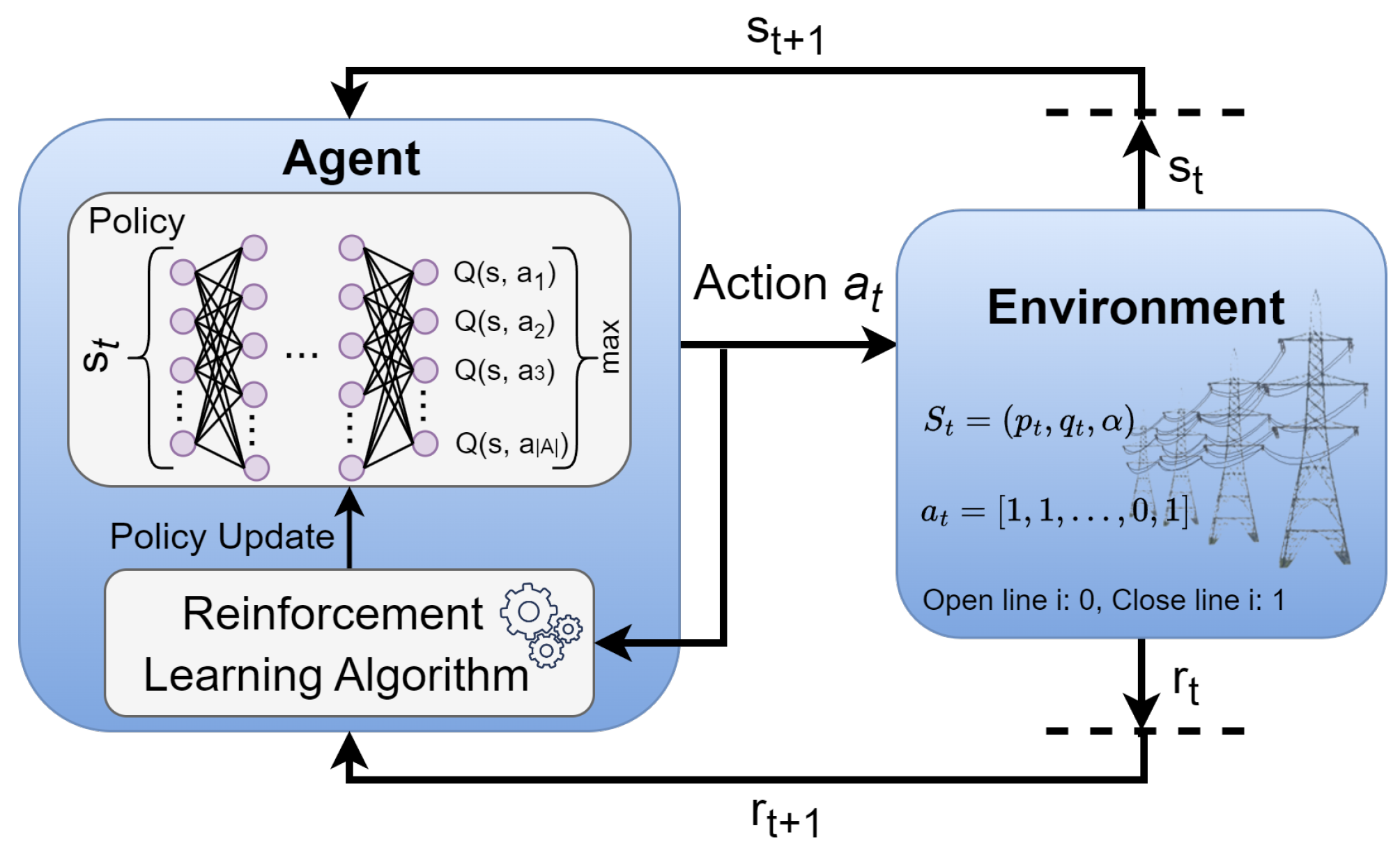
Figure 1. Schematic diagram showing how RL works.
Energies 17 05187 g001
Figure 2. Active power losses for a fully connected 33-node test system.
Energies 17 05187 g002
Figure 3. The 33-node system’s sorted active power loss for 50,751 actions (top) and 1000 actions with maximum loss (bottom).
Energies 17 05187 g003
Figure 4. The 119-node system’s sorted active power loss for 3,500,000 actions (top) and 2000 actions with maximum loss (bottom).
Energies 17 05187 g004
Figure 5. The 136-node system’s sorted active power loss for 3,500,000 actions (top) and 2000 actions with maximum loss (bottom).
Energies 17 05187 g005
Figure 6. The mean daily rewards (top) and their 60-step moving average (bottom) for 33-node system during training.
Energies 17 05187 g006
Figure 7. The mean daily rewards (top) and their 60-step moving average (bottom) for 119-node system during training.
Energies 17 05187 g007
Figure 8. The mean daily rewards (top) and their 60-step moving average (bottom) for 136-node system during training.
Energies 17 05187 g008
Figure 9. The 60-step moving average of daily rewards for 33-node system with a varying number of actions.
Energies 17 05187 g009
Figure 10. The 60-step moving average of daily rewards for 119-node system with a varying number of actions.
Energies 17 05187 g010
Figure 11. The 60-step moving average of daily rewards for 136-node system with a varying number of actions.
Energies 17 05187 g011
Figure 12. RL agent’s response to unforeseen loads in the 33-node system.
Energies 17 05187 g012
Figure 13. RL agent’s response to unforeseen loads in the 119-node system.
Energies 17 05187 g013
Figure 14. RL agent’s response to unforeseen loads in the 136-node system.
Energies 17 05187 g014
Figure 15. System loss and voltage penalty for various R l values in 136-node system.
Energies 17 05187 g015
Table 1. DQN and dueling DQN parameters.
ParameterValue
Learning rate ( α ) 0.001
Batch size (b)512
Discount factor ( γ ) 0.99
Neural network structure { 1024 , 1024 }
Experience replay memory size 30,000,000
Table 2. Tie switches of the DNR result for a single hour in 33-node system.
AlgorithmTie SwitchesSystem Loss [kW]
DQN7-8, 10-11, 14-15, 28-29, 32-33140.71
Dueling DQN7-8, 9-10, 14-15, 28-29, 32-33139.98
Table 3. Tie switches of the DNR result for a single hour in 119-node system.
AlgorithmTie SwitchesSystem Loss [kW]
DQN23-24, 32-33, 72-73, 109-110, 46-27,1025.98
17-27, 54-43, 62-49, 37-62, 9-40, 58-96,
88-75, 99-77, 108-83, 105-86
Dueling DQN20-21, 34-35, 72-73, 109-110, 46-27,1015.04
17-27, 54-43, 62-49, 37-62, 9-40,
58-96, 88-75, 99-77, 108-83, 105-86
Table 4. Tie switches of the DNR result for a single hour in 136-node system.
AlgorithmTie SwitchesSystem Loss [kW]
DQN47-62, 89-90, 105-106, 134-135,288.84
46-27, 7-73, 9-24, 15-83, 25-51,
50-96, 55-98, 66-79, 79-131, 84-135,
91-104, 90-129, 92-104, 92-132,
96-120, 126-76, 128-77, 135-98
Dueling DQN31-35, 48-51, 89-90, 106-107,294.33
7-73, 9-24, 15-83, 50-96, 55-98,
62-120, 66-79, 79-131, 84-135,
91-104, 90-129, 92-104, 92-132,
96-120, 126-76, 128-77, 135-98
Table 5. Computational speed comparison.
AlgorithmExecution Time [s]
33 Buses119 Buses136 Buses
DQN 0.21 0.88 0.78
Dueling DQN 0.21 0.88 0.79
BCSAC [24] 0.4 2.2 -
NoisyNet DQN [32] 0.48 --
SOE [35]1 12.3 16.9
MIQP [15] 3.2 39.4 188.4
AACO [5] 0.3 430.74 894.20
MP [35]1940071236
Approximate RL
Training Time
15,14545,45453,000
Table 6. Loss and minimum voltage comparison for different methods.
AlgorithmTest System
33 Nodes119 Nodes136 Nodes
LossVoltageLossVoltageLossVoltage
DQN 140.70 0.94 958.90 0.93 285.34 0.96
Dueling DQN 139.98 0.94 954.62 0.93 286.32 0.96
SOE [35] 139.55 0.94 853.58 0.93 280.94 0.96
MIQP [15] 139.55 0.94 871.23 0.93 261.97 0.96
AACO [5] 139.55 0.94 865.86 0.93 279.75 0.96
MP [35] 139.55 - 853.58 - 280.14 -
FPEO [38] 140.33 0.94 861.19 0.93 - -
FHA [39] 139.55 - - - 280.19 -
No DNR 202.68 0.91 1298.09 0.87 320.36 0.93
Optimality gap0.3%10.58%1.95%
Disclaimer/Publisher’s Note: The statements, opinions and data contained in all publications are solely those of the individual author(s) and contributor(s) and not of MDPI and/or the editor(s). MDPI and/or the editor(s) disclaim responsibility for any injury to people or property resulting from any ideas, methods, instructions or products referred to in the content.