Article

Recurrence Multilinear Regression Technique for Improving Accuracy of Energy Prediction in Power Systems

by
Quota Alief Sias
1,
Rahma Gantassi
1,
Yonghoon Choi
1,* and
Jeong Hwan Bae
2
1
Department of Electrical Engineering, Chonnam National University, Gwangju 61186, Republic of Korea
2
Department of Economics, Chonnam National University, Gwangju 61186, Republic of Korea
*
Author to whom correspondence should be addressed.
Energies 2024, 17(20), 5186; https://doi.org/10.3390/en17205186
Submission received: 13 September 2024 / Revised: 9 October 2024 / Accepted: 15 October 2024 / Published: 18 October 2024
(This article belongs to the Section F: Electrical Engineering)

Abstract

:
This paper demonstrates how artificial intelligence can be implemented in order to predict the energy needs of daily households using both multilinear regression (MLR) and single linear regression (SLR) methods. As a basic implementation, the SLR makes use of one input variable, which is the total amount of energy generated as an input. The MLR implementation involves multiple input variables being taken from various energy sources, including gas, coal, geothermal, wind, water, biomass, oil, etc. All of these variables are derived from detailed energy production data from the various energy sources. The purpose of this paper is to demonstrate that it is possible to analyze energy demand and supply directly together as a way to produce a more in-depth analysis. By analyzing energy production data from previous periods of time, a prediction of energy demand can be made. Compared to the SLR implementation, the MLR implementation is found to perform better because it is able to achieve a smaller error value. Furthermore, the forecasting pattern is carried out sequentially based on a periodic pattern, so this paper calls this method the recurrence multilinear regression (RMLR) method. This paper also creates a pre-clustering using the K-Means algorithm before the energy prediction to improve accuracy. Other models such as exponential GPR, sequential XGBoost, and seq2seq LSTM are used for comparison. The prediction results are evaluated by calculating the MAE, RMSE, MAPE, MAPA, and time execution for all models. The simulation results show that the fastest and best model that obtains the smallest error (3.4%) is the RMLR clustered using a weekly pattern period.

1. Introduction

An energy system flows energy from generators on the supply side to consumers on the demand side, with the settings and monitoring carried out by an energy management system (EMS). An EMS can be on a small scale, for example, a single house [1] with several generating sources such as solar panels, grids, and generators [2]. An EMS can also be implemented on a larger scale, such as a city [3] or country [4], with all energy sources distributing electricity to consumers, as shown in Figure 1. Consumers on the demand side use the EMS to save electricity costs, while power generation companies on the supply side use the EMS to ensure that the energy generation process is efficient. A power plant must ensure that there are enough energy sources available to meet the energy needs of consumers. Power system operations require the accurate prediction of energy demand (known as load forecasting) due to the simultaneous generation and consumption of electric power [5]. The results of the load forecasting process can also be used to generate the amount of electricity needed to match the amount of load consumed. A lack of precision in forecasting electrical loads can result in blackouts that partially or entirely disable the power grid. Excess power generation can result in economic losses if overestimations are made. In light of its importance, several studies have been conducted on energy demand forecasting. The load forecast can be based on historical data from the energy demand as univariate [6] and can involve other factors such as weather, seasonal patterns, or other multivariate factors [7].
The load forecast can be divided into long-term load forecast [8], medium-term load forecast for up to several months [9,10], and short-term forecast of less than one day (hourly or minutely) [11,12]. There are many models that can be used to forecast loads, including regression models. Regression models are still top-rated because they are simple and produce good prediction accuracy. The simplest model is linear regression [13], which has also been implemented to forecast daily peak loads in South Korea. Linear models are very suitable when all features have a reasonable correlation. The model often consists of only one variable [14] using a single linear regression model. Subsequently, it became a multivariate model using a multilinear regression [15]. A multivariate model can be implemented by a multivariate output [16] or a multivariate input [17]. Using multivariate data certainly requires many new features as input variables to the regression model. Generally, load forecasting only uses historical data from the load as time series data, which involve the use of only one variable from the load side [18]. Predictions on the supply side, such as renewable energy generation [19], rarely involve load data in their analysis. Supply and load predictions can simultaneously provide more complete and complementary information on the EMS [20].
There are many regression models, and one that has been proven to have the best performance compared to many other regression models is exponential Gaussian process regression (GPR) [12]. The sequential XGBoost model can also be used as a comparison, which is also based on multivariate data for long-term predictions and can cope with the fluctuating nature of peak power demand during these periods [21]. The best model for different time series machine learning methods that are often used is sequential long short-term memory (LSTM) [22,23]. The LSTM model provides good performance for daily energy prediction [24] and becomes more accurate by using a multistep time series in seq2seq LSTM [25]. The newest model that can further increase precision is the use of K-Means to group data [26] during the forecasting process [27]. Single models are certainly faster in the prediction process, while multi-models provide more accurate forecasting opportunities [28]. Although hybrid techniques have the potential to be more accurate, fundamental models, such as linear regression, can still provide the best prediction results [29].
For all models to make energy forecasts, elements that are often added as parameters to strengthen prediction accuracy are the weather [30], seasons, and holiday patterns [31]. These parameters are often obtained from different sources or companies that are sometimes not open to the public. Because these parameters often differ from country to country, it is not always possible to use the same model in different places. This paper discusses the implementation of the K-Means algorithm in recursive load forecasting models with daily, weekly, monthly, and quarterly patterns. In order to make a daily energy prediction, the energy data from the previous day are used as a reference. When a forecast is made weekly, the prediction for a specific day on a particular day refers to the same day from the previous week. The process of predicting the demand for energy on a monthly and quarterly basis is processed similarly. Exponential GPR, sequential XGBoost, and seq2seq LSTM are used as comparison models to validate the prediction results. The prediction results of all models are evaluated using error calculations to show the accuracy of their predictions. This paper explains how to build an energy demand prediction model using multivariate data of historical energy supply. This paper also combines periodic patterns to improve the prediction results. Because it is based only on periodic patterns, the simulation results can conclude on the best pattern to make predictions, and the proposed model is expected to be applied in all countries without weather or season constraints. Based on the proposed model for carrying out load forecasting, this paper has the following contributions:
  • This paper proposes the energy supply (production) as an input data model (coal, gas, oil, nuclear, river, wind, solar, etc.) to predict energy demand (consumption).
  • It develops a multilinear regression model from a single linear regression to implement a multivariate input model.
  • It also combined the K-Means clustering algorithm and multilinear regression to make fewer errors.
  • It uses periodic daily, weekly, monthly, and quarterly patterns to improve the accuracy of energy prediction.

2. Proposed RMLR Model and Evaluation

The data of energy demand (consumption) and energy supply (generation) of the electrical system based on open data in Turkey [17] consist of several energy resources as shown in Figure 2. The correlation between energy consumption and energy production is perfectly matched if there are no losses of energy based on the conservation of energy laws, as expressed in (1). W s u p p l y represents energy generation consisting of several energy resources. W d e m a n d represents the energy load from consumers. W l o s s expresses the energy that changes to other energy, such as heat, when electricity is transferred from the generator to the consumer. If load forecasting on time series data only uses historical load data, while the energy load trend historically always increases every time, the next prediction result will definitely also increase and need a limiter as a constraint. Equation (1) explains the importance of analyzing demand and supply simultaneously because in reality, energy consumption cannot exceed energy generation. In reality, there is a loss of energy due to many factors, for example, the loss of energy in the transmission and distribution line. If the energy loss is constant, it is inevitable that an increase in energy demand also leads to an increase in energy supply and vice versa. The energy demand is not allowed to exceed the supply energy and is limited by circuit breakers for each electricity user. The circuit breaker is used not only for the safety of electricity users but also for the safety of the generator side. Although the trend for energy demand throughout the world is increasing, this cannot be realized in every country because the energy supply has limits, and the generators also have limits to their capabilities.
W s u p p l y = W d e m a n d + W l o s s
Generally, there is more than one type of energy source used to supply electrical energy to consumers. Based on the data in this article, a correlation between each source of energy supply, total energy supply, and energy demand is shown in Figure 3. The total energy supply and the energy demand have an almost perfect linear correlation value of 0.98 according to the law of energy conservation. A very high positive value in this correlation indicates that the two variables are very strongly correlated; for example, if there is a slight increase in energy demand, the energy supply will also increase. According to (1), a perfect correlation value is impossible because there is always energy loss. Another condition that makes it not perfect is the inaccuracy of measurements or missing data in the EMS. If the total energy supply is broken down, each energy source contributes a different correlation value to the energy demand. Gas energy sources have a correlation value of 0.55, which is the highest level of linearity with respect to energy demand compared to other energy sources. The total energy supply and each energy supply source are used as a single variable and multivariate feature in the model of an energy demand forecaster.

2.1. The Proposed RMLR Techniques

Datetime, pandas, numpy, scikit-learn, seaborn, matplotlib, and plotly were among the Python libraries used in data preparation, model development, and evaluation. A regression equation involving one independent input variable and one dependent output variable is represented in (2) where the variable x represents the input, and the variable y represents the output. Using the SLR model, we can find one of the intercept values α 0 and one of the slope values α 1 . Multilinear regression models are described in (3), where multiple independent variables are input, and a single dependent output variable is used. Due to the MLR model’s input value also containing more than one value, the slope value is also more than one. The proposed model is based on the MLR model because it can reduce the error value more than the SLR model as it has more than one slope.
y = α 0 + α 1 x
y = α 0 + α 1 x 1 + α 2 x 2 + α 3 x 3
Data from historical seven-year periods were used to develop a model for energy use and production in Turkey considering coal, gas, geothermal, hydro, biomass, wind, oil, and others. The output variable of the models was the forecast of energy consumption in all training data. An SLR model took into account the total energy generation from all sources as a single input variable. MLR models were constructed on the basis of the energy produced by various energy sources. A regression model was used to predict the result once the slope and intercept values were obtained. The method of recurrence regression was described as a periodic forecasting process. The performance of the energy demand model was determined by the difference between the predictions and the actual historical data.
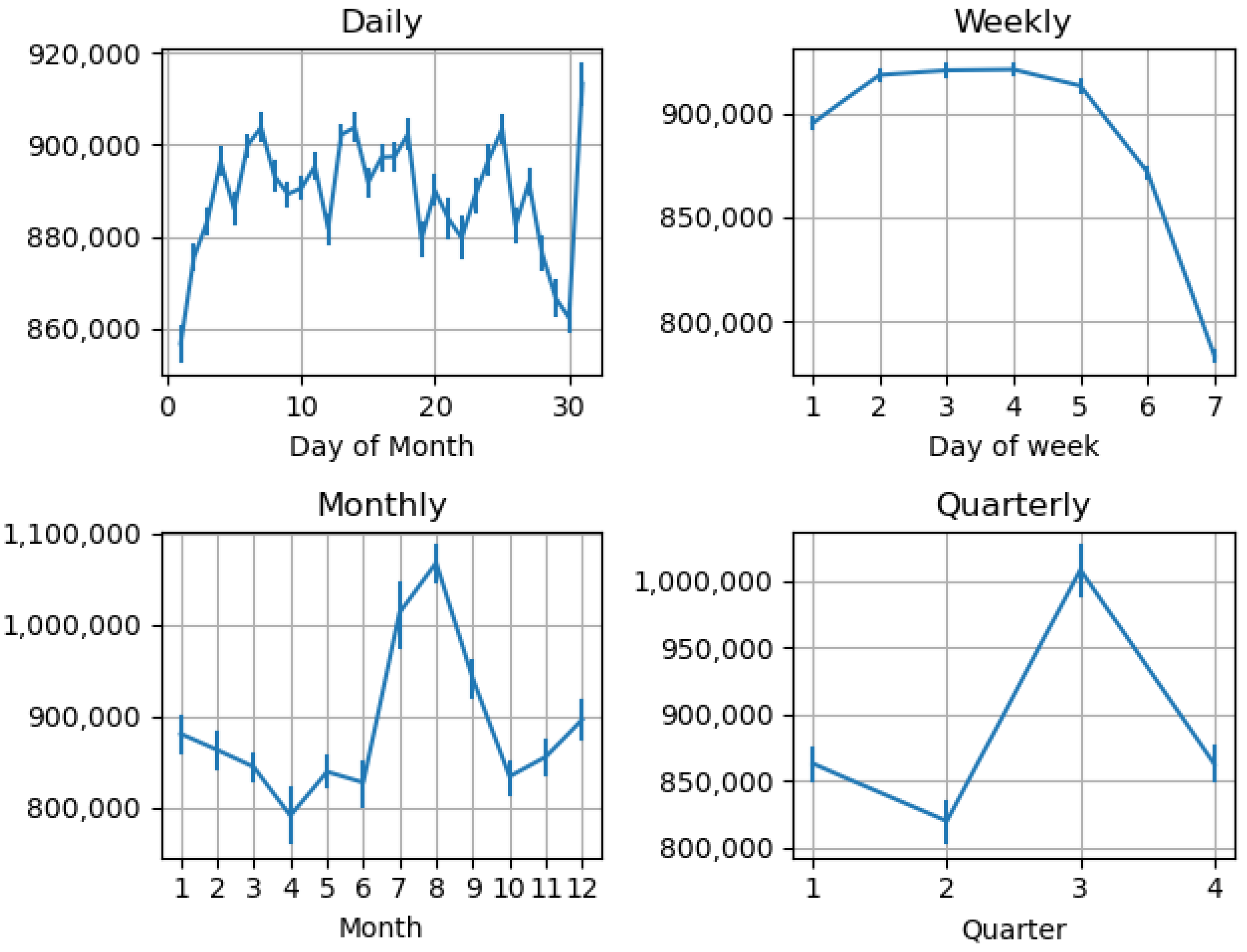
Four periodic patterns were used in all models for energy forecasting in this paper. Figure 4 illustrates how the energy consumption patterns were divided according to the previous day in the month (day of the month), the weekday (day of the week), the day of the month (the same month) and the quarter day (the same quarter). Data from the previous day were used to predict energy usage on a daily basis. On a weekly basis, energy predictions also referred to the same day the previous week, and on a quarterly basis, the process was similar. The proposed periodic patterns are common repetition patterns that can be applied to all countries. In the daily pattern, it indicates that the training or testing data only used historical data on the same day on the date of the previous month. The weekly pattern involved making predictions using data from the corresponding day of the previous week. For example, the prediction for Monday was based solely on the data from the previous Monday. In the monthly pattern, the prediction for January was based on the previous January in previous years, and so were the other months’ predictions. Although the quarter pattern can represent a country with four seasons, the prediction for this year’s winter was only based on the data from the previous year’s winter, and so were the other seasons’ predictions.
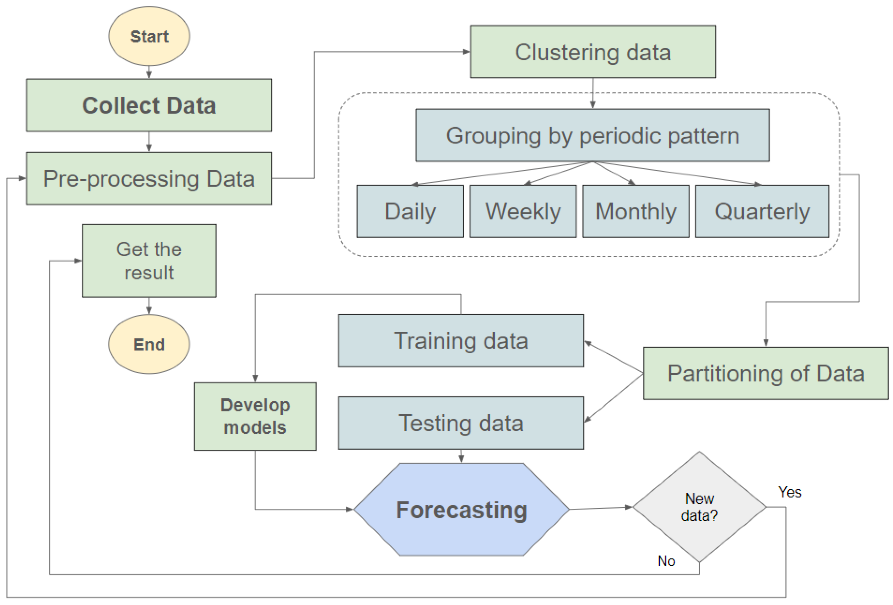
Apart from dividing data based on periodic patterns, pre-clustering was performed using the K-Means algorithm. This clustering was used to obtain clusters from historical energy data in the forecasting process. Variable y represents the output (total energy load), load forecasting, and x represents the inputs: a single variable (total energy supply) for SLR, or multiple variables (each energy resource) for MLR. This article used simulations of both SLR and MLR models to highlight the advantages of MLR over SLR. All training data were used to obtain intercept α 0 and slope values ( α 1 , α 2 , α 3 , etc.) for the SLR and MLR models for each cluster and grouping result. The test data were also partitioned based on clusters and groupings of the four periodic patterns selected for the forecast. The four proposed periodic patterns were tested for all selected models and used to find the best pattern. A detailed explanation is given in Algorithm 1, which explains the details of the SLR or MLR implementation based on Equations (2) and (3). Figure 5 explains the flowchart used in this article. The first step was to collect historical data on energy generation and consumption. The next step was to preprocess the data so that the data were valid and complete without missing data. After that, the data were clustered and grouped according to the proposed periodic pattern. Data partitioning was performed for each group. The model was built and trained on the basis of its group using training data. Furthermore, load forecasting was performed with test data according to the group. If there were new data, the data were also be preprocessed and grouped prior to the prediction process.
Algorithm 1 Clustering RMLR algorithm
Energies 17 05186 i001

2.2. Model Performance Evaluation

An evaluation of a model can be carried out by calculating the root-mean-square error (RMSE), the mean average error (MAE), the mean average percentage error (MAPE), the mean average percentage accuracy (MAPA) of the model, and the execution time. The MAPE is the same as the MAE when expressed as a percentage and when compared with the model as a whole. The MAPA is calculated by subtracting 100% accuracy from the MAPE in order to calculate the accuracy of the model. The MAPA is a measure of how accurately the model predicts the outcome, while the MAE and RMSE measure how far the model is from the actual value. All of these metrics are important to consider when evaluating a model’s performance.
  • All calculated errors are divided by the square root of the mean to obtain the RMSE. The forecast error is a measure of prediction accuracy, measured as the difference between forecast and actual data.
    RMSE = x = 1 X ( Y t Y t ^ ) 2 X
  • The MAE represents the average error of all the forecasting results from the training data. The error is calculated based on a comparison between the predicted and actual electricity demand.
    MAE = x = 1 X | Y t Y t ^ | 2 X
  • Using data from forecast results, the MAPE can be used to calculate the average error as a percentage. For the error percentage, the mean value of the prediction results compared to the actual electricity demand is multiplied by 100%.
    MAPE = x = 1 X | Y t Y t ^ | Y t X × 100 %
  • The mean absolute percentage accuracy is the model prediction accuracy value. MAPA is obtained after calculating the error percentage value with a perfect accuracy of 100% minus the total average error percentage obtained.
MAPA = 100 % MAPE
X is the total quantity of all predicted data starting from x = 1. Y t ^ represents the energy forecast by the models, while Y t represents the energy used under actual conditions.

3. Simulation Results

In renewable energy systems such as wind [32] or photovoltaic [33] systems, establishing a reliable and precise day-to-day energy forecast is crucial for the EMS. To construct the model, this article used electrical data from Turkey from 2017 to 2023 on energy consumption and production resulting from various energy sources (gas, coal, geothermal, hydro, wind, biomass, oil, etc.). Essentially, this paper focused on historical energy data that could be broken down into daily energy data, so it could be used as a reference and a guide for making monthly and yearly predictions for energy consumption. Hourly data were recorded and collected to obtain daily data from both the production side and the electricity consumption side. These data were added 24 h in advance to obtain daily data from demand and supply on both sides.

3.1. Data Preprocessing

A total of 59,856 rows and 21 columns were included in the final dataset, which was a representation of historical daily performance data relating to energy consumption and production collected over a period of seven years. It was calculated from the raw data by adding the values of energy consumption every 24 h to arrive at the daily value of energy consumption. All data were confirmed to be complete (no missing data), and no errors were reported as a result. The data were converted into the same data type and proven to be valid, making it easier to perform further data processing and analysis to help obtain further information using the data.This research minimized uncertainty with confidence intervals for coefficients and prediction intervals for forecasting. There is a higher uncertainty associated with wider intervals, either due to data noise or model limitations. Therefore, a narrower prediction interval indicates a lower uncertainty in the prediction of the model, as it indicates a higher degree of confidence [34].
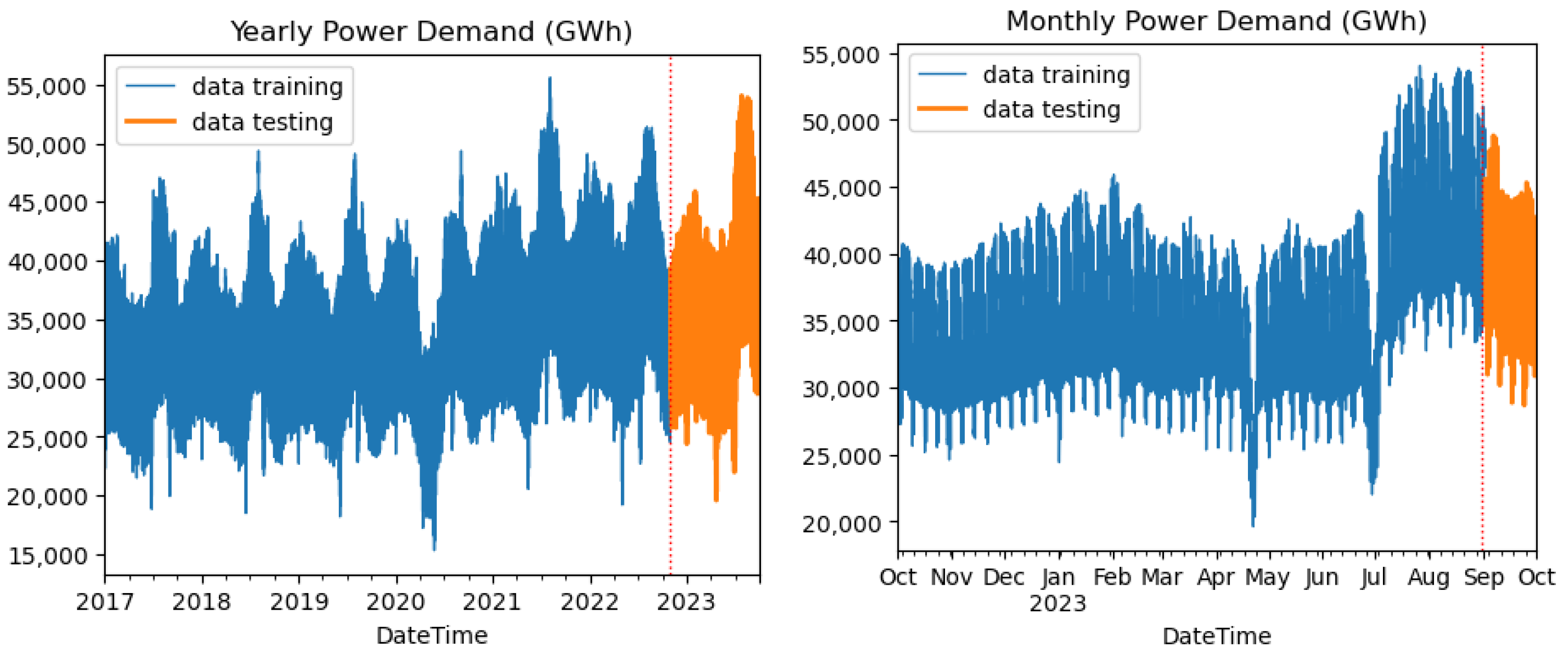
Data in this article were divided into a smaller number of test sets of less than thirty percent [35] of the whole dataset in order to allow a fair comparison of load forecasting. Detailed data on historical energies were divided into two parts so that a model could be created based on these data, as shown in Figure 6. Predictions for a year were based on training data over the course of six years and testing data over the course of one year. When it came to making monthly predictions, the training process used eleven months of data, and the testing process used one month of testing data. The SLR model was developed by following the preparation of the data according to (2), and the MLR model was developed according to (3). After the data were prepared, the K-Means clustering technique was used before making predictions based on the RMLR model and period patterns.

3.2. Clustering Multilinear Regression

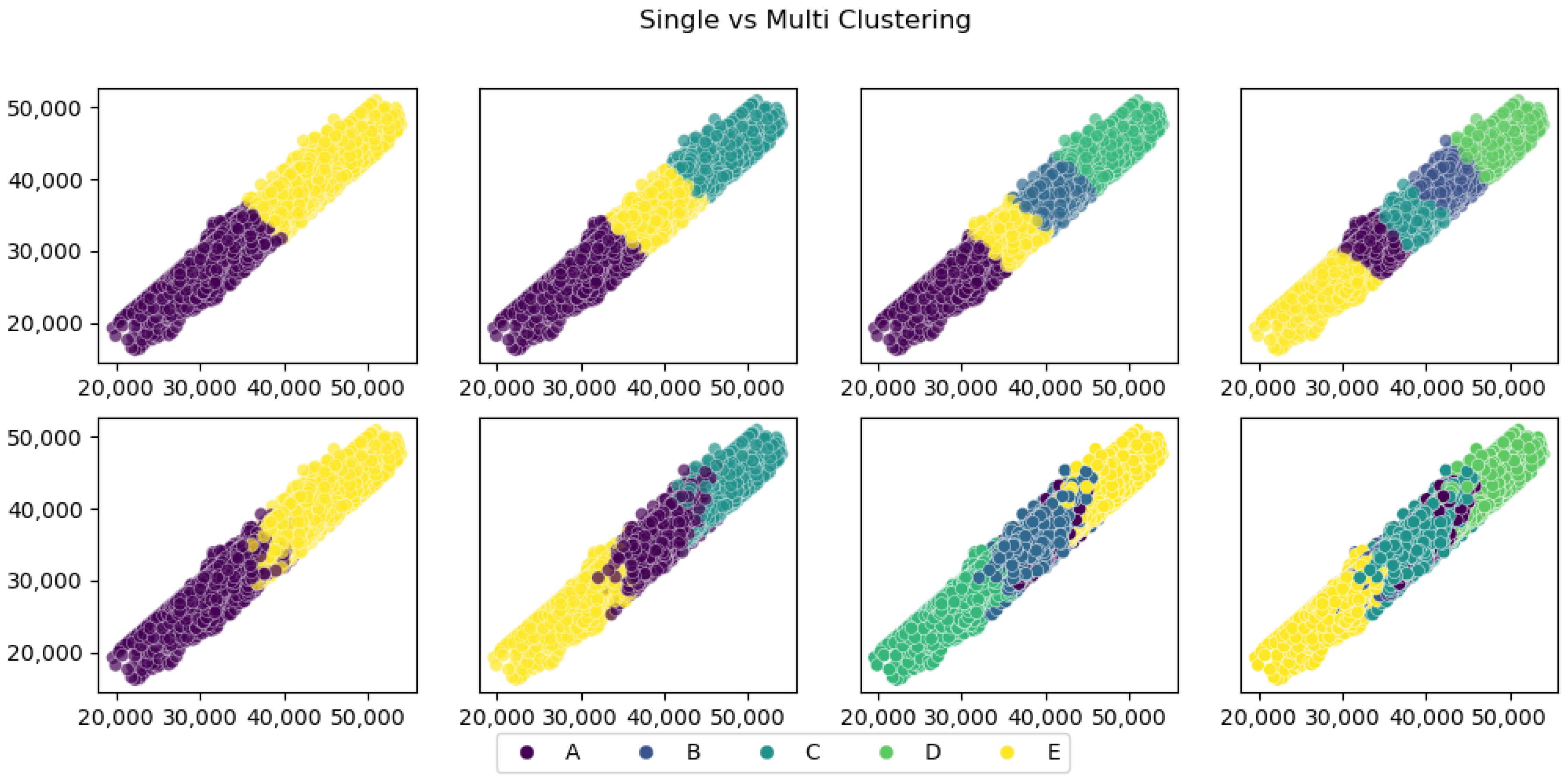
As a method to predict the load using machine learning, the K-Means clustering algorithm was used in the proposed method. It is an unsupervised learning technique that divides a dataset into K distinct pairs of data points that do not overlap. Based on K-Means, similar data points are grouped together and assigned to the same cluster so that the variance within each cluster is minimized. The implementation of the K-Means algorithm can use single variables and multiple variables. The authors in [36] selected five clusters as the optimum number using the gap statistic for load forecasting in PV systems. Other authors [37] also used K-Means clustering to obtain the optimal number of clusters, which was five for the daily characteristic factor data collected based on the CH index (the relationship between the degree of separation and the compactness of the dataset). In [25], the authors also mentioned the goodness of fit of the number of clusters for our multistep time series clustering algorithm by using the Silhouette score, from two to four clusters, showing two clusters fitted the business and school load curves. Figure 7 explains the clusters that were created based on the energy data, which consisted of two to five clusters. For single variables, the total energy supply was used as an input variable compared to the energy demand as an output variable to produce clusters that were distributed proportionally based on distance. For multiple variables, each energy source was used as a multivariate input to calculate the cluster distance, so that the clusters appeared random even though they were actually still based on proportional distances from each input variable.
The performance of the model was evaluated using the error metrics expressed in (4)–(7). Table 1 lists all the error metrics, such as MAE, RMSE, and MAPE. The errors were calculated for single-variable and multivariate K-Means clustering for each cluster pattern given by each clustering algorithm. The results show that the performance of the MLR compared to the SLR was always better because it had a small error. The best number of clusters, especially for the MLR model, was only two clusters with an MAE error value of 19,019 MWh for single-variable clustering and 16,337 for multivariate clustering. This result also showed that multivariate clustering was a better solution than single-variable clustering and that it was an effective solution to improve the proposed model. Additionally, the use of the MLR model could be improved using a multivariate K-mean with two clusters. Multivariate clustering could also be used to identify outliers and patterns in the data.
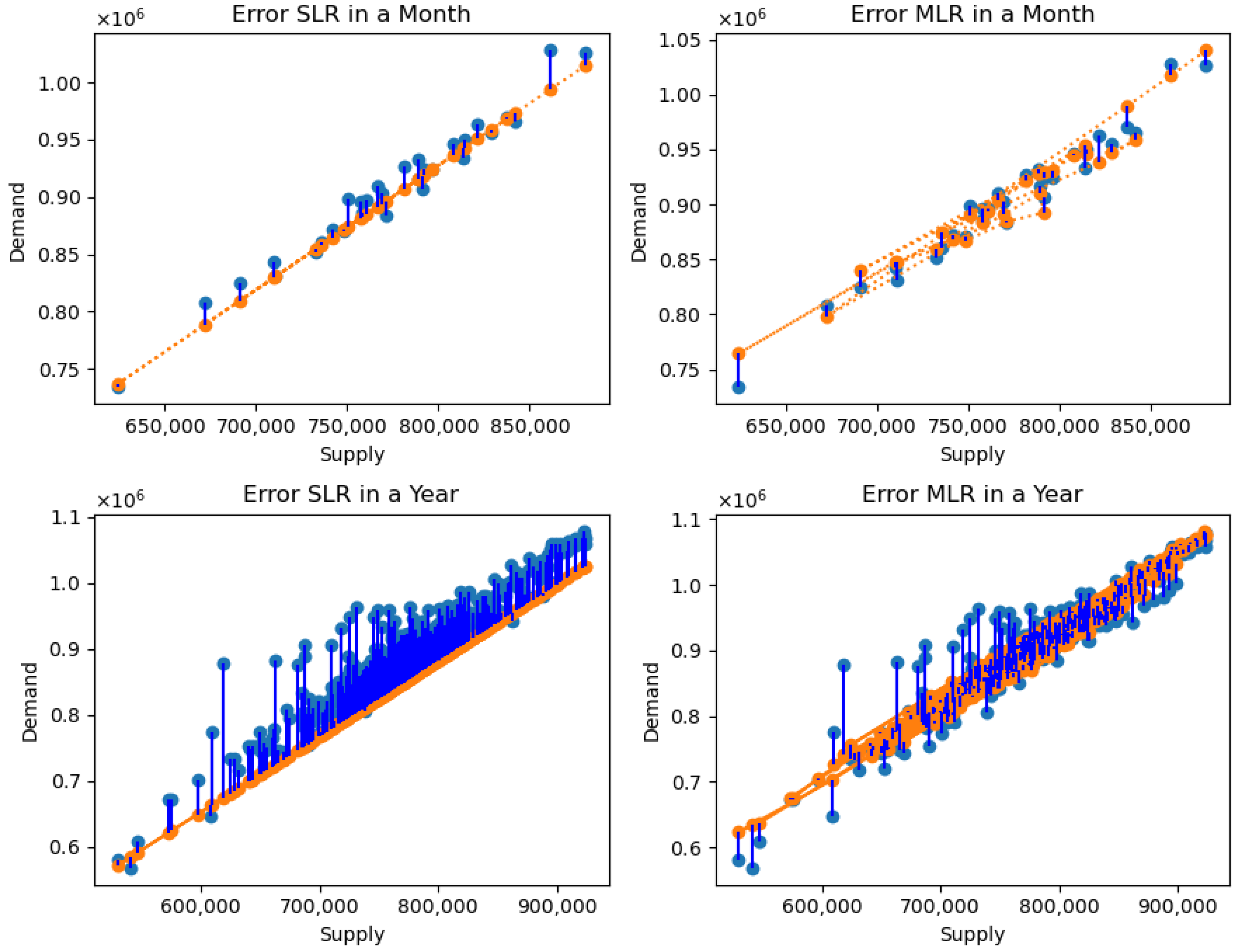
Since MLR has multiple slope values in addition to a single slope value, MLR has the potential to produce better predictions compared to SLR. The monthly and annual prediction curves can be seen in Figure 8; the SLR shows only a single line of descent while the MLR has more than one slope value, which depends on the number of energy values that are sent as input variables from each of the energy sources. There is definitely a possibility that whenever there is more than one slope value, the error value can be lower because all of the energy sources have a direct or indirect influence on the total amount of energy sent to consumers. This means that the accuracy of the MLR model can be improved by taking into account the multiple energy sources. Furthermore, this can also be beneficial for energy suppliers and consumers as the model can provide more accurate predictions and estimates.

3.3. Comparison with Other Methods

To compare the performance of the proposed model, the following models were used: exponential GPR, sequential XGBoost, and seq2seq LSTM. Details about the exponential GPR model can be found in [12], and those for the sequential XGBoost can be found in [21]. Ref. [25] provides an explanation of the parameters involved in the construction of the seq2seq LSTM model used to generate the model mentioned above. Recursive load forecasting models based on these patterns were developed and applied to daily, weekly, monthly, or quarterly forecasting models. Table 2 lists the MAE, RMSE, MAPE, and MAPA for all models’ predictions based on pattern periods. According to the simulation results, all models produced excellent forecasts with an accuracy of more than 99% on average. The proposed model obtained the smallest error values, 91.304 MWh for the RMSE and 91.201 MWh for the MAE. This RMLR model showed the best results when using the proposed pattern for the weekly data period using the proposed model. The execution time on the same model was influenced by how much data were used; the less data used, the faster the time required for prediction. The monthly pattern was the fastest because it only used one month’s data from each year, followed by the quarterly pattern which used four months’ data in one year. Daily patterns almost had the same speed as weekly data because the data could be used on all days only from day 1 until 28. The weekly pattern was the best because it used data from all days and captured repeating patterns every week.
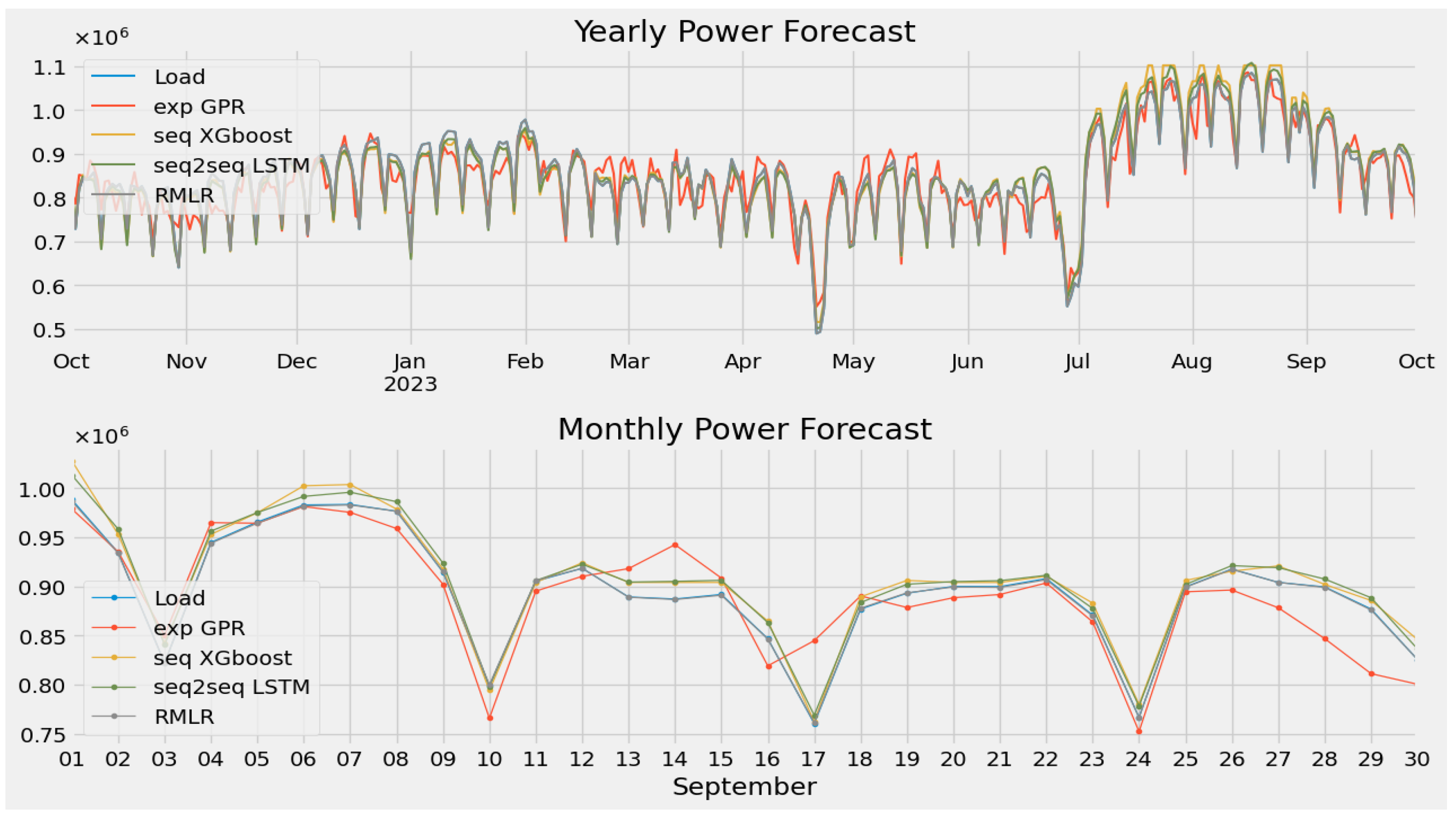
Based on test data, the average error value for all models was based on the forecast results and actual data from 2023, which covered a one-year period. The MAE and RMSE were found to be the same in units of MWh and were plotted side by side, as shown in Figure 9. The MAPE is a percentage error expressed in the form of a percentage value, which is a measure of the MAE based on error Formula (6). Figure 9 shows the average error value of all period patterns from all models presented in Table 2. The best model was RMLR, with an error value of 91.304 MWh for the RMSE and 91.201 MWh for MAE. In terms of RMSE, the exponential GPR (91.293 MWh) and sequential XGBoost (92.441 MWh) were the next best performing models, and in terms of MAE, it was the seq2seq LSTM model with 109.518 MWh. Figure 10 shows the results of the daily energy predictions over a period of one month and one year based on the distribution of training and testing data previously described in Figure 6. The fastest prediction time was also obtained from the proposed MLMR model because it used a simple single fundamental model of linear regression. The proposed model outperformed other models because it used a multivariate input and combined K-Means techniques with periodic patterns. All models can be used to predict daily loads in monthly and annual periods, and the resulting prediction curve can always follow the actual value of the energy demand.

4. Conclusions

An in-depth analysis of the correlation between energy demand and supply can be achieved by analyzing them directly together to produce an energy forecast. Energy consumption can be predicted by regression models based on energy production data from previous periods. It was found that multiple variables using the MLR implementation performed better than single variables on the SLR implementation since it achieved a better prediction. In addition, this paper used a K-Means algorithm to pre-cluster data before predicting energy demand using regression models. Other models used for comparison were exponential GPR, sequential XGBoost, and seq2seq LSTM models. This paper used recurrence multilinear regression to forecast daily energy based on periodic patterns. Recursive load forecasting models were developed using these patterns on a daily, weekly, monthly, or quarterly basis. To evaluate the precision of the predicted results, the RMSE, the MAE, the MAPE, the MAPA, and the execution time were calculated for all models. Based on the simulation results, it was shown that a clustered RMLR was the fastest, and using a weekly pattern period produced the best model, obtaining the smallest errors. All models proposed in this paper could be used to forecast daily load energy with an accuracy of more than 99% and obtained a prediction result that followed the actual energy demand. This paper still used a fundamental model with a new method of preprocessing data using multivariate combinations with clustering and periodic patterns. This technique can also be applied in various parts of the world because of the ease of obtaining data such as climate, weather, or other external data. However, to upgrade the model for future research, using the latest advanced deep learning models will be necessary. They can be hybrid models or ensemble learning and expand the model to include external variables such as weather conditions, political data, social data, etc. Implementing these techniques in the EMS will help optimize the energy system according to the actual demand response conditions. Implementing optimization techniques in models can save energy costs, especially if connected to energy trading in the energy system.

Author Contributions

The research was carried out successfully with contribution from all authors. The main research idea and manuscript preparation were contributed by Q.A.S.; Y.C., R.G. and J.H.B. contributed to the manuscript preparation and gave several suggestions from industrial perspectives. All authors have read and agreed to the published version of the manuscript.

Funding

This work was supported by the Ministry of Education of the Republic of Korea and the National Research Foundation of Korea (NRF-2023S1A5C2A07096111).

Data Availability Statement

The original contributions presented in the study are included in the article, further inquiries can be directed to the corresponding author.

Conflicts of Interest

The authors declare no conflicts of interest.

References

  1. Aurangzeb, K.; Alhussein, M. Deep learning framework for short term power load forecasting, a case study of individual household energy customer. In Proceedings of the International Conference on Advances in the Emerging Computing Technologies (AECT), Madinah, Saudi Arabia, 10 February 2020; pp. 1–5. Available online: https://ieeexplore.ieee.org/abstract/document/9194153 (accessed on 20 September 2023).
  2. Parkash, B.; Lie, T.T.; Li, W.; Tito, S.R. End-to-End Top-Down Load Forecasting Model for Residential Consumers. Energies 2024, 17, 2550. [Google Scholar] [CrossRef]
  3. Tang, L.; Yi, Y.; Peng, Y. An ensemble deep learning model for short-term load forecasting based on ARIMA and LSTM. In Proceedings of the IEEE International Conference on Communications, Control, and Computing Technologies for Smart Grids (SmartGridComm), Beijing, China, 21–23 October 2019; pp. 1–6. Available online: https://ieeexplore.ieee.org/abstract/document/8909756 (accessed on 20 September 2023).
  4. Sias, Q.A.; Lim, S.; Gantassi, R.; Choi, Y. Implementation of Single and Multi Linear Regression for Prediction of Energy Consumption based on Previous Data of Energy Production. In Proceedings of the 2023 International Conference on Artificial Intelligence in Information and Communication (ICAIIC), Bali, Indonesia, 20–23 February 2023; pp. 830–832. Available online: https://ieeexplore.ieee.org/document/10066989 (accessed on 20 September 2023).
  5. Alquthami, T.; Zulfiqar, M.; Kamran, M.; Milyani, A.H.; Rasheed, M.B. A Performance Comparison of Machine Learning Algorithms for Load Forecasting in Smart Grid. IEEE Access 2022, 10, 48419–48433. [Google Scholar] [CrossRef]
  6. Zhu, J.; Dong, H.; Zheng, W.; Li, S.; Huang, Y.; Xi, L. Review and prospect of data-driven techniques for load forecasting in integrated energy systems. Appl. Energy 2022, 321, 119269. [Google Scholar] [CrossRef]
  7. Habbak, H.; Mahmoud, M.; Metwally, K.; Fouda, M.M.; Ibrahem, M.I. Load Forecasting Techniques and Their Applications in Smart Grids. Energies 2023, 16, 1480. [Google Scholar] [CrossRef]
  8. Lindberg, K.B.; Seljom, P.; Madsen, H.; Fischer, D.; Korpås, M. Long-term electricity load forecasting: Current and future trends. Util. Policy 2019, 58, 102–119. [Google Scholar] [CrossRef]
  9. Alkawaz, A.N.; Abdellatif, A.; Kanesan, J.; Khairuddin, A.S.M.; Gheni, H.M. Day-Ahead Electricity Price Forecasting Based on Hybrid Regression Model. IEEE Access 2022, 10, 108021–108033. [Google Scholar] [CrossRef]
  10. Sharma, A.; Jain, S.K. A novel seasonal segmentation approach for day-ahead load forecasting. Energy 2022, 257, 124752. [Google Scholar] [CrossRef]
  11. Huy, P.C.; Minh, N.Q.; Tien, N.D.; Quynh, T. Short-term Electricity Load forecasting based on Temporal Fusion Transformer Model. IEEE Access 2022, 10, 106296–106304. [Google Scholar] [CrossRef]
  12. Madhukumar, M.; Sebastian, A.; Liang, X.; Jamil, M.; Khan, S. Regression Model-Based Short-Term Load Forecasting for University Campus Load. IEEE Access 2022, 10, 8891–8905. [Google Scholar] [CrossRef]
  13. Lee, G.-C. Regression-Based Methods for Daily Peak Load Forecasting in South Korea. Sustainability 2022, 14, 3984. [Google Scholar] [CrossRef]
  14. Kareem, S.; Akpinar, M. Removing Seasonal Effect on City Based Daily Electricity Load Forecasting with Linear Regression. In Proceedings of the International Symposium on Networks, Computers and Communications (ISNCC), Dubai, United Arab Emirates, 31 October–2 November 2021; pp. 1–6. Available online: https://ieeexplore.ieee.org/abstract/document/9615873 (accessed on 26 October 2023).
  15. Ardiansyah; Masood, Z.; Choi, D.; Choi, Y. Seq2Seq regression learning-based multivariate and multistep SOC forecasting of BESS in frequency regulation service. Sustain. Energy Grids Netw. 2022, 32, 100939. [Google Scholar] [CrossRef]
  16. Selvi, M.V.; Mishra, S. Investigation of Performance of Electric Load Power Forecasting in Multiple Time Horizons with New Architecture Realized in Multivariate Linear Regression and Feed-Forward Neural Network Techniques. IEEE Trans. Ind. Appl. 2020, 56, 5603–5612. [Google Scholar] [CrossRef]
  17. Sias, Q.A.; Gantassi, R.; Choi, Y.; Afandi, A. Recurrence Multi Linear Regression of Historical Energy Supply for Energy Demand Forecaster. In Proceedings of the 2023 8th International Conference on Electrical, Electronics and Information Engineering (ICEEIE), Malang City, Indonesia, 28–29 September 2023; pp. 1–4. Available online: https://ieeexplore.ieee.org/abstract/document/10334912 (accessed on 26 October 2023).
  18. Mohammadi, E.; Alizadeh, M.; Asgarimoghaddam, M.; Wang, X.; Simões, M.G. A Review on Application of Artificial Intelligence Techniques in Microgrids. IEEE J. Emerg. Sel. Top. Ind. Electron. 2022, 3, 878–890. [Google Scholar] [CrossRef]
  19. Patel, R.K.; Kumari, A.; Tanwar, S.; Hong, W.-C.; Sharma, R. AI-Empowered Recommender System for Renewable Energy Harvesting in Smart Grid System. IEEE Access 2022, 10, 24316–24326. [Google Scholar] [CrossRef]
  20. Cai, H.; Shen, S.; Lin, Q.; Li, X.; Xiao, H. Predicting the Energy Consumption of Residential Buildings for Regional Electricity Supply-Side and Demand-Side Management. IEEE Access 2019, 7, 30386–30397. [Google Scholar] [CrossRef]
  21. Zhang, T.; Zhang, X.; Rubasinghe, O.; Liu, Y.; Chow, Y.H.; Iu, H.H.C.; Fernando, T. Long-term Energy and Peak Power Demand Forecasting based on Sequential-XGBoost. IEEE Trans. Power Syst. 2023, 39, 3088–3104. [Google Scholar] [CrossRef]
  22. Suresh, V.; Aksan, F.; Janik, P.; Sikorski, T.; Revathi, B.S. Probabilistic LSTM-Autoencoder Based Hour-Ahead Solar Power Forecasting Model for Intra-Day Electricity Market Participation: A Polish Case Study. IEEE Access 2022, 10, 110628–110638. [Google Scholar] [CrossRef]
  23. Neeraj; Mathew, J.; Behera, R.K. EMD-Att-LSTM: A Data-driven Strategy Combined with Deep Learning for Short-term Load Forecasting. J. Mod. Power Syst. Clean Energy 2022, 10, 1229–1240. [Google Scholar] [CrossRef]
  24. Qi, Y.; Luo, H.; Luo, Y.; Liao, R.; Ye, L. Adaptive Clustering Long Short-Term Memory Network for Short-Term Power Load Forecasting. Energies 2023, 16, 6230. [Google Scholar] [CrossRef]
  25. Masood, Z.; Gantassi, R.; Ardiansyah; Choi, Y. A Multi-Step Time-Series Clustering-Based Seq2Seq LSTM Learning for a Single Household Electricity Load Forecasting. Energies 2022, 15, 2623. [Google Scholar] [CrossRef]
  26. Shafique, T.; Gantassi, R.; Soliman, A.-H.; Amjad, A.; Hui, Z.-Q.; Choi, Y. A Review of Energy Hole Mitigating Techniques in Multi-Hop Many to One Communication and its Significance in IoT Oriented Smart City Infrastructure. IEEE Access 2023, 11, 121340–121367. [Google Scholar] [CrossRef]
  27. Dong, X.; Deng, S.; Wang, D. A short-term power load forecasting method based on k-means and SVM. J. Ambient. Intell. Humaniz. Comput. 2022, 13, 5253–5267. [Google Scholar] [CrossRef]
  28. Mamun, A.A.; Sohel, M.; Mohammad, N.; Sunny, M.S.H.; Dipta, D.R.; Hossain, E. A Comprehensive Review of the Load Forecasting Techniques Using Single and Hybrid Predictive Models. IEEE Access 2020, 8, 134911–134939. [Google Scholar] [CrossRef]
  29. Asghar, Z.; Hafeez, K.; Sabir, D.; Ijaz, B.; Syed; Ro, J. RECLAIM: Renewable Energy Based Demand-Side Management Using Machine Learning Models. IEEE Access 2023, 11, 3846–3857. [Google Scholar] [CrossRef]
  30. Mehedi, I.M.; Bassi, H.M.; Rawa, M.; Ajour, M.N. Intelligent Machine Learning with Evolutionary Algorithm Based Short Term Load Forecasting in Power Systems. IEEE Access 2021, 9, 100113–100124. [Google Scholar] [CrossRef]
  31. Permata, R.P.; Prastyo, D.D.; Wibawati. Hybrid dynamic harmonic regression with calendar variation for Turkey short-term electricity load forecasting. Procedia Comput. Sci. 2022, 197, 25–33. [Google Scholar] [CrossRef]
  32. Wang, W.; Feng, B.; Huang, G.; Guo, C.; Liao, W.; Chen, Z. Conformal asymmetric multi-quantile generative transformer for day-ahead wind power interval prediction. Appl. Energy 2023, 333, 120634. [Google Scholar] [CrossRef]
  33. Wang, L.; Mao, M.; Xie, J.; Liao, Z.; Zhang, H.; Li, H. Accurate solar PV power prediction interval method based on frequency-domain decomposition and LSTM model. Energy 2023, 262, 125592. [Google Scholar] [CrossRef]
  34. Sluijterman, L.; Cator, E.; Heskes, T. How to evaluate uncertainty estimates in machine learning for regression? Neural Netw. 2024, 173, 106203. [Google Scholar] [CrossRef]
  35. Zhang, Y.; Wen, H.; Wu, Q.; Ai, Q. Optimal adaptive prediction intervals for electricity load forecasting in distribution systems via reinforcement learning. IEEE Trans. Smart Grid 2022, 14, 3259–3270. [Google Scholar] [CrossRef]
  36. Sleiman, A.; Su, W. Combined K-Means Clustering with Neural Networks Methods for PV Short-Term Generation Load Forecasting in Electric Utilities. Energies 2024, 17, 1433. [Google Scholar] [CrossRef]
  37. Zeng, W.; Li, J.; Sun, C.; Cao, L.; Tang, X.; Shu, S.; Zheng, J. Ultra Short-Term Power Load Forecasting Based on Similar Day Clustering and Ensemble Empirical Mode Decomposition. Energies 2023, 16, 1989. [Google Scholar] [CrossRef]
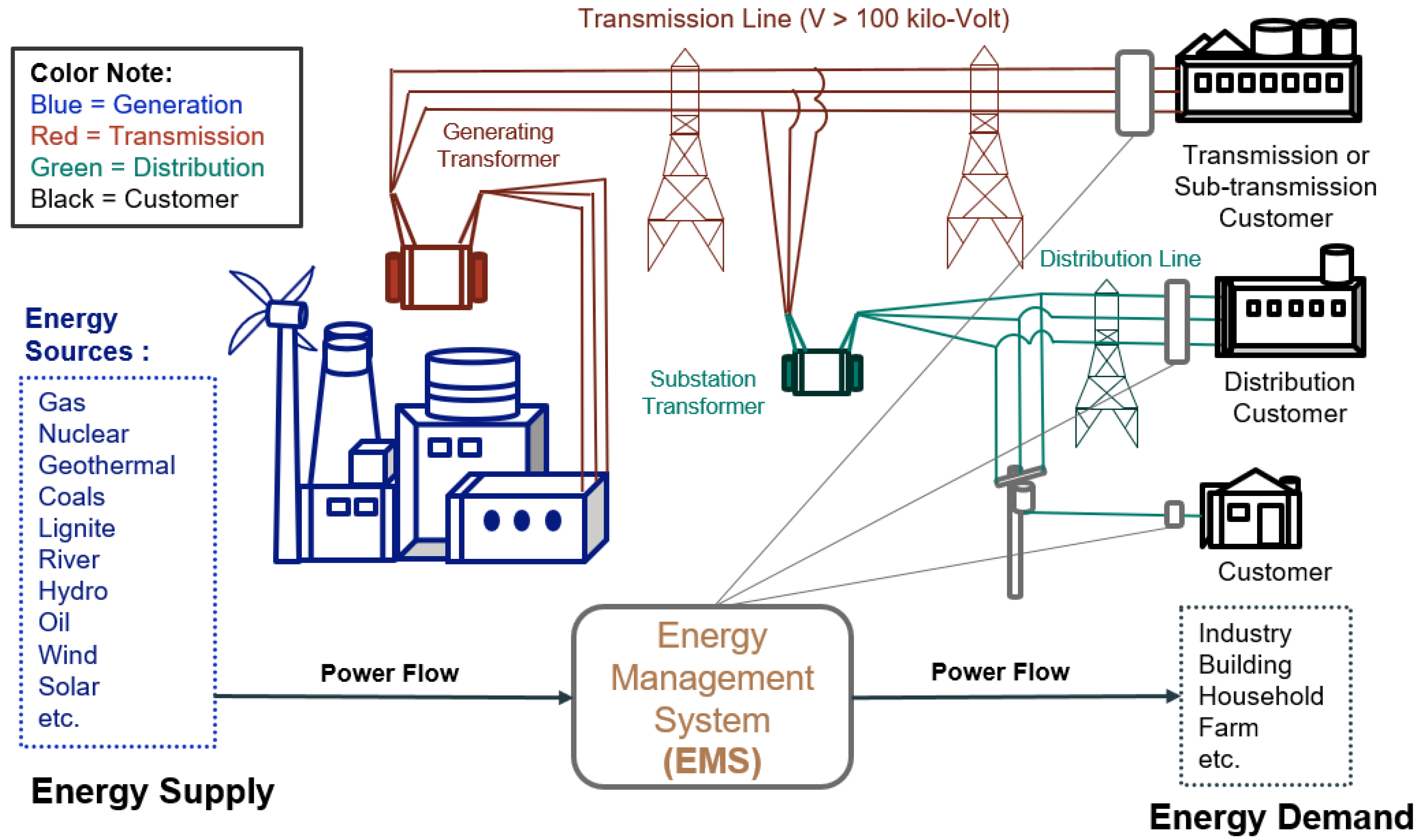
Figure 1. Energy transmission within the power system via the EMS.
Energies 17 05186 g001
Figure 2. The sources of electrical power generation.
Energies 17 05186 g002
Figure 3. The correlation between a set of features in the dataset.
Energies 17 05186 g003
Figure 4. Recurring patterns of energy consumption over the past seven years (GWh).
Energies 17 05186 g004
Figure 5. A flowchart of the methodology in this research.
Energies 17 05186 g005
Figure 6. Splitting the dataset of electrical energy for training and testing the models.
Energies 17 05186 g006
Figure 7. Energy demand vs. supply for single and multivariate clustering.
Energies 17 05186 g007
Figure 8. SLR vs. MLR prediction energy performance.
Energies 17 05186 g008
Figure 9. Error values of real and predicted energy from testing data.
Energies 17 05186 g009
Figure 10. Yearly and monthly energy prediction from testing data.
Energies 17 05186 g010
Table 1. Errors from the MLR and SLR clustering.
ErrorModel2345
Single-variable clustering
MAESLR46.16746.05847.13648.002
MLR19.01921.34019.87024.500
RMSESLR54.69254.22356.05856.239
MLR28.84631.49630.17634.517
MAPESLR0.05480.05470.05330.0533
MLR0.02190.02490.02310.0278
Multivariate clustering
MAESLR48.26346.75546.24349.043
MLR16.33720.18330.09026.048
RMSESLR55.24652.28651.70454.825
MLR25.81927.44137.18734.520
MAPESLR0.05400.05290.05250.0553
MLR0.01850.02330.03490.0295
Table 2. Performance results of the models.
ModelRMSEMAEMAPEMAPATime
Daily
exp GPR99.849123.5330.10999.8901.986
seq XGboost101.325122.6790.10999.8900.127
seq2seq LSTM100.665119.1570.10999.89122.243
RMLR92.72691.8550.04799.9530.24
Weekly
exp GPR91.293111.0490.10099.9002.124
seq XGboost92.441111.4390.09999.9100.212
seq2seq LSTM96.526109.5180.10599.89522.873
RMLR91.30491.2010.03499.9660.37
Monthly
exp GPR96.889112.8940.10799.8931.337
seq XGboost102.172115.3960.03699.9640.098
seq2seq LSTM98.324111.6200.10799.89320.991
RMLR91.61391.3250.03699.9640.004
Quarterly
exp GPR100.604117.0500.11099.8901.549
seq XGboost101.661117.0460.10899.8920.103
seq2seq LSTM106.171119.1740.11499.88621.461
RMLR91.51191.3650.03899.9620.011
Error values are in MWh and time is in seconds.
Disclaimer/Publisher’s Note: The statements, opinions and data contained in all publications are solely those of the individual author(s) and contributor(s) and not of MDPI and/or the editor(s). MDPI and/or the editor(s) disclaim responsibility for any injury to people or property resulting from any ideas, methods, instructions or products referred to in the content.