Multiple Load Forecasting of Integrated Renewable Energy System Based on TCN-FECAM-Informer

Abstract

In order to solve the problem of complex coupling characteristics between multivariate load sequences and the difficulty in accurate multiple load forecasting for integrated renewable energy systems (IRESs), which include low-carbon emission renewable energy sources, in this paper, the TCN-FECAM-Informer multivariate load forecasting model is proposed. First, the maximum information coefficient (MIC) is used to correlate the multivariate loads with the weather factors to filter the appropriate features. Then, effective information of the screened features is extracted and the frequency sequence is constructed using the frequency-enhanced channel attention mechanism (FECAM)-improved temporal convolutional network (TCN). Finally, the processed feature sequences are sent to the Informer network for multivariate load forecasting. Experiments are conducted with measured load data from the IRES of Arizona State University, and the experimental results show that the TCN and FECAM can greatly improve the multivariate load prediction accuracy and, at the same time, demonstrate the superiority of the Informer network, which is dominated by the attentional mechanism, compared with recurrent neural networks in multivariate load prediction.

1. Introduction

In order to cope with the energy and environmental crises, energy transition is imperative, and integrated renewable energy systems (IRESs) have become an important method of energy utilization in the process of energy transition by bringing the links between various energy systems closer. Therefore, the development of integrated renewable energy systems will be an important method of energy utilization in the future. IRESs emphasize the integration of the generation, conversion, storage, distribution, and consumption of multiple forms of energy [1], which can greatly improve the utilization rate of energy. Unlike traditional energy systems that consider a single load forecast, IRESs need to consider a multivariate load forecast that contains complex coupled information, which puts higher requirements on the accuracy of the load forecast.

1.1. Related Work

The key to improving the accuracy of load forecasting lies in the selection of load forecasting models and the extraction of valid information from raw data. In terms of load forecasting model selection, it can be mainly categorized into traditional machine learning and deep learning methods.

For traditional machine learning, Ref. [2] proposes a predictive model for power load forecasting based on phase space reconstruction and support vector machine (SVM). Ref. [3] uses LSSVM combined with the multitask learning weight sharing mechanism for IRES multivariate load forecasting, and Ref. [4] analyzes a variety of regression models by comparing them, and ultimately recommends the use of the Gaussian process regression model for power load forecasting.

Deep learning methods use multi-layer neural network stacking to construct models for load forecasting. Ref. [5] developed a complex neural network (ComNN) for multivariate load forecasting. Ref. [6] utilized a long short-term neural network (LSTM) combined with genetic algorithms (GAs) for pre-training, and then fine-tuned it using transfer learning to build a multivariate load forecasting model GA-LSTM. Ref. [7] proposed a multivariate load prediction model combining the transformer and Gaussian process.

In order to further improve the overall performance of the model and fully exploit the effective information of relevant features and historical load data, signal decomposition techniques and convolutional neural networks are applied in load forecasting.

For signal decomposition techniques, Ref. [8] utilized the backpropagation (BP) neural network for the initial load prediction and utilized improved complete ensemble empirical mode decomposition with adaptive noise (ICEEMDAN) to decompose and reconstruct the results, before utilizing the gated recurrent unit (GRU) algorithm for the further prediction of the reconstructed components and combining it with the prediction results of the BP neural network. Ref. [9] proposed a two-stage decomposition hybrid forecasting model for the multivariate load forecasting of IRESs by combining modal decomposition with the bidirectional long short-term memory neural network (Bi-LSTM). Ref. [10] utilized variational mode decomposition (VMD) with the k-means clustering algorithm (FK) combined with the SecureBoost model for the forecasting of electricity load, and Ref. [11] used a combination of complete ensemble empirical mode decomposition with adaptive noise (CEEMDAN) and VMD to form a secondary mode decomposition. CEEMDAN decomposes the load sequence into multiple subsequences, while VMD further decomposes the high-frequency components for multivariate load prediction. Ref. [12] combines ICEEMDAN and successive variational mode decomposition (SVMD) to form an aggregated hybrid mode decomposition (AHMD) for modal decomposition, and after that, the multivariate linear regression (MLR) model is used, respectively, with the temporal convolutional network-bidirectional gated recurrent unit (TCN-BiGRU) fusion neural network for the prediction of low-frequency components and medium–high-frequency components, respectively, and the prediction results are superimposed for IES load prediction. In Ref. [13], modal decomposition is combined with the multitask learning model; the middle- and high-frequency sequences of multivariate loads after modal decomposition are input into the multitask transformer model for prediction; the low-frequency sequences are input into the multitask bi-directional gated logic recurrent unit for prediction; and the results of the two are ultimately superimposed to obtain the final prediction results.

In terms of the convolutional neural network, Ref. [14] performed feature extraction by fusing the convolutional neural network (CNN) and GRU, followed by a multitask learning approach to build a multivariate load prediction model. Ref. [15] utilized the multi-channel convolutional neural network (MCNN) to extract high-dimensional spatial features and combined it with the LSTM network for IRES load prediction. Ref. [16], on the other hand, used a three-layer CNN to extract features, followed by load prediction using the transformer model.

The analysis of the previous related research revealed the following aspects that can be improved in the research related to multivariate load forecasting:

(1)

Most of the different feature extraction methods use traditional modal decomposition and convolutional neural networks, and more advanced networks can be further adopted and improved to enhance the model’s feature analysis capability and improve the model’s performance.

(2)

Most of the deep prediction models in the research use traditional recurrent neural networks, and attempts can be made to use other types of network structures to capture correlations between sequences and to improve the ability of deep prediction models to parallelize the computation and the learning of long-term dependencies of sequences.

Therefore, a multivariate load forecasting model combining an improved time-series convolutional TCN and Informer network is proposed for multivariate load prediction. First, the channel attention mechanism (CAM) and discrete cosine transform (DCT) are combined with the TCN to improve the feature processing capability of the model. Second, the overall prediction model is constructed by combining the Informer network. Finally, by considering an arithmetic example, the model’s effectiveness in multivariate load forecasting is demonstrated.

1.2. Contributions

(1)

The CAM and DCT are combined with TCN for feature analysis. The CAM and DCT enhance the extraction of key features, and the TCN is responsible for the modeling of time series to lay the foundation for the next prediction.

(2)

The Informer network combined with the improved TCN is applied to the prediction of multivariate loads, and the feasibility of the network model of the encoder–decoder framework, which is dominated by the attention structure in the deep prediction model, is verified for the multivariate load prediction.

(3)

This paper uses the MIC method to analyze the correlation between multivariate loads and other factors such as meteorology mainly in order to analyze the correlation between multivariate loads and other factors, and to make the selection of features for the input model.

The next part of this paper focuses on the following: the second part introduces the TCN model, the improvement module, and the subsequent Informer network model used for predicting, and proposes an overall modeling framework for improving the TCN combined with the Informer network. In the third part, the effectiveness of the proposed model is analyzed using practical examples. Finally, conclusions are drawn and future plans are outlined.

2. The Principles of the Relevant Methods

2.1. TCN Model

The TCN is a deep learning network structure, which is very different from traditional neural networks. Its structure is based on a one-dimensional convolutional neural network, which can effectively extract the correlation between data by integrating various mechanisms such as inflationary convolution, causal convolution, and the residual module, and can better deal with time series prediction problems [17].

The core of the TCN is the inflated causal convolution. Causal convolution is a unidirectional structure, i.e., the output at a point in time at the previous level is only relevant to the input at that point in time and earlier at the next level. The sense field of causal convolution is linearly related to the depth of the network, which requires a deeper network structure and longer training time when dealing with long history information, resulting in causal convolution not being able to effectively capture information from long time series. Therefore, the TCN uses the expansion convolution to sample the input data at intervals, which is calculated as shown in Equation (1).

$$F(t)={\displaystyle {\sum }_{i=0}^{k-1}f(i)}\cdot x_{t-d\cdot i}$$

(1)

$F$ is the convolution operation, $F(t)$ is the output value at time point $t$, $k$ is the size of the convolution kernel, $f(i)$ is the $i$ element in the convolution kernel, and $x_{t-d\cdot i}$ is the input value corresponding to shifting from the $t$ moment to the past $d\cdot i$ moment.

The expansion coefficient of inflated causal convolution grows exponentially with the increase in the number of layers, which in turn expands the receptive fields, enabling the model to capture local features on different time scales, thus improving the modeling capability for time-series data. And local features are the patterns and regularities captured within these limited receptive fields. However, compared to ordinary convolutional networks, TCNs have a reduced number of layers, but they are able to obtain a larger receptive field, thus avoiding the repeated extraction of information and being able to fully analyze the features of the data.

As the number of layers increases, the expansion coefficient increases exponentially, which in turn expands the receptive fields, allowing the model to capture local features on different time scales. And local features are the patterns and regularities captured within these limited receptive fields. However, compared with the ordinary convolutional network, the TCN is reduced in the number of layers, but it is able to obtain a larger receptive field, thus avoiding the repeated extraction of information and being able to fully analyze the characteristics of the data.

In addition, traditional neural networks are prone to gradient explosion and network degradation when the number of layers is gradually deepened, so the residual connectivity module [18] is applied in the output layer of the TCN. In Figure 1, the residual connectivity module structure is shown. The module consists of two identical internal units and a one-dimensional convolutional network, where the internal units include the expansion causal convolutional layer, the normalization layer, the activation function, and the dropout layer.

2.2. Frequency-Enhanced Channel Attention Mechanism (FECAM)

The FECAM is an improvement in CAM. The CAM has been applied in CNNs. In the squeeze-and-excitation (SE) module [19], the relationships between different channels of the feature map are modeled using global information, and the feature map is re-modified to improve its representational ability. However, the frequency domain information of the data extracted by the Fourier transform in channel attention can introduce high-frequency components due to the period problem, thus affecting the feature extraction. The FECAM uses the DCT [20] instead of the Fourier transform to avoid the above problem. The steps of the FECAM are as follows:

First, the FECAM splits each input feature map along the channel dimension into $n$ subgroups as $V^i=\left\{v_0,v_1,\dots ,v_{n-1}\right\}$. Then, the DCT is performed on all the components of each subgroup, where each single channel is subjected to the same frequency of components to obtain Equation (2):

$$Fre{q}^i=DC{T}_j(V^i)={\displaystyle {\sum }_{j=0}^{j=L_s}({V^i}_l)}{B}_l^j$$

(2)

$$B_l^{\mathrm{j}}=\cos ({\displaystyle \frac{\pi l}{L_s}}(j+{\displaystyle \frac{1}{2}}))$$

(3)

where $l\in \{0,1,\dots ,L_s-1\}$, $i\in \left\{0,1,\dots ,n-1\right\}$, and $j\in \left\{0,1,\dots ,L_S-1\right\}$, in which $j$ are the frequency component 1D indices corresponding to $V^i$, and $Fre{q}^i\in R^L$ is the $L$-dimensional vector after the discrete cosine transformation.

Then, the whole frequency channel vector can be obtained by stack operation.

$$Freq=DCT(V)=stack([Fre{q}^0,Fre{q}^1,\dots ,Fre{q}^{n-1}])$$

(4)

where $Freq\in R^{C\times L}$, $V\in R^{C\times L}$, and $Freq$ is the attention vector of $V$.

The whole equations for the entire frequency-enhanced attention mechanism is as follows:

$$F_c-att=\sigma (W_2\delta (W_{1}DCT(V)))$$

(5)

$$att=\sigma (W_2\delta (W_{1}Z))$$

(6)

$$Zc=GAP(x_c)={\displaystyle \frac{1}{L_S}}{\displaystyle \sum _{i=1}^{L_S}{x}_c(i)}$$

(7)

In Equation (4), $\sigma$ and $\delta$ are RELU and Sigmoid activation functions, and $W_1$ and $W_2$ are the two fully connected layers. In Equation (5), $att$ is the learned attention vector that can be scaled for each channel of data, $Z$ consists of $Zc$ from different channels; in Equation (6), $Z_c$ is obtained by scaling the inputs $x$ in the temporal dimension, and $L_S$ is the length of the time-series sequence.

Through the frequency-enhanced channel attention mechanism, each channel feature interacts with each frequency component to comprehensively obtain important temporal information from the frequency domain and enhance the diversity in information of features extracted by the network.

2.3. Informer Network

The whole architecture of the Informer network is an encoder–decoder architecture.

The main role of the encoder is to uncover information about the features of the input data, and its core modules are the Prob-Sparse self-attention mechanism and distillation operation. The Prob-Sparse self-attention mechanism receives either the input or the output of the previous encoder, and multiplies the received data by different weights to obtain the three matrices $Q$, $K$, and $V$. The Prob-Sparse self-attention module is

$$A(Q,K,V)=Soft\max ({\displaystyle \frac{\overline{Q}{K}^T}{\sqrt{d}}})V$$

(8)

where $Q$ is the improved query matrix, $K$ is the attention content, and $\overline{Q}{K}^T$ calculates the attention weight of $Q$ on $V$.

The distillation operation assigns higher weights to dominant features with dominant attention. From the $j$ layer to $j+1$, the distillation operation is as follows:

$$X_{j+1}^t=MaxPool(ELU(Conv1d({\left[X_j^t\right]}_{AB})))$$

(9)

${[\cdot ]}_{AB}$ is the attention module, and the one-dimensional convolution on the time series is denoted by $\mathrm{Conv}1\mathrm{d}[\cdot ]$. This is followed by maximum pooling after passing the activation function ELU.

The decoder is mainly responsible for processing the feature information obtained from the encoder, and finally outputting the result through the fully connected layer.

2.4. Maximum Information Coefficient (MIC)

The Maximum Information Coefficient can be used to represent a linear or nonlinear relationship between two variables, with a wide range of applicability and low computational complexity. The MIC takes a value in the range of 0–1, and the closer it is to 1, the stronger the correlation.

The basic principle of the MIC is that if there is a correlation between two variables, a grid can be plotted on a scatterplot consisting of two variables and the MIC can be calculated using MI (Mutual Information) and grid partitioning. The specific steps for correlation analysis using the MIC are as follows.

First, let the weather factor variable be $A=\left\{a_i\right\}(i=1,2,3,\dots ,n)$ and the multivariate load variable be $B=\left\{b_j\right\}(j=1,2,\dots ,m)$, where $n$ and $m$ are the number of weather factor and multivariate load variables, respectively. The formula for calculating the MI value is as follows:

$$f_{M1}(A,B)={\displaystyle \sum _{a_i\in A}{\displaystyle \sum _{b_j\in B}p(a_i,b_j)}}{\log }_2{\displaystyle \frac{p(a_i,b_j)}{p(a_i)p(b_j)}}$$

(10)

where $p(a_i,b_j)$ is the joint probability density of variables $a_i$ and $b_j$, and $p(a_i)$ and $p(b_j)$ are the marginal probability densities of variables $a_i$ and $b_j$, respectively.

Second, define a grid, denoted as $G\left(x,y\right)$; divide $a_i$ and $b_j$ in the dataset $D=\left\{(a_i,b_j)\right\}$ into two grids, $x$ and $y$, respectively; and compute to obtain the maximum MI value of $D$ under the division of the grid $G$:

$$f_{M1}(D,x,y)=\max f_{M1}(D|G)$$

(11)

where $f_{M1}(D|G)$ is the MI value of dataset $D$ under $G$.

Third, for a fixed dataset $D$, all the maximum MI values of different grids $G$ on $D$ are normalized to the (0, 1) interval, and the normalization is calculated as follows:

$$M{(D)}_{x,y}={\displaystyle \frac{f_{M1}(D,x,y)}{{\log }_2\min \left\{x,y\right\}}}$$

(12)

Finally, MIC is the normalized maximum MI value and is calculated as follows:

$$f_{MIC}=\underset{\left|x\right|\left|y\right|<B}{\max }\left\{M{(D)}_{x,y}\right\}$$

(13)

2.5. TCN-FECAM-Informer

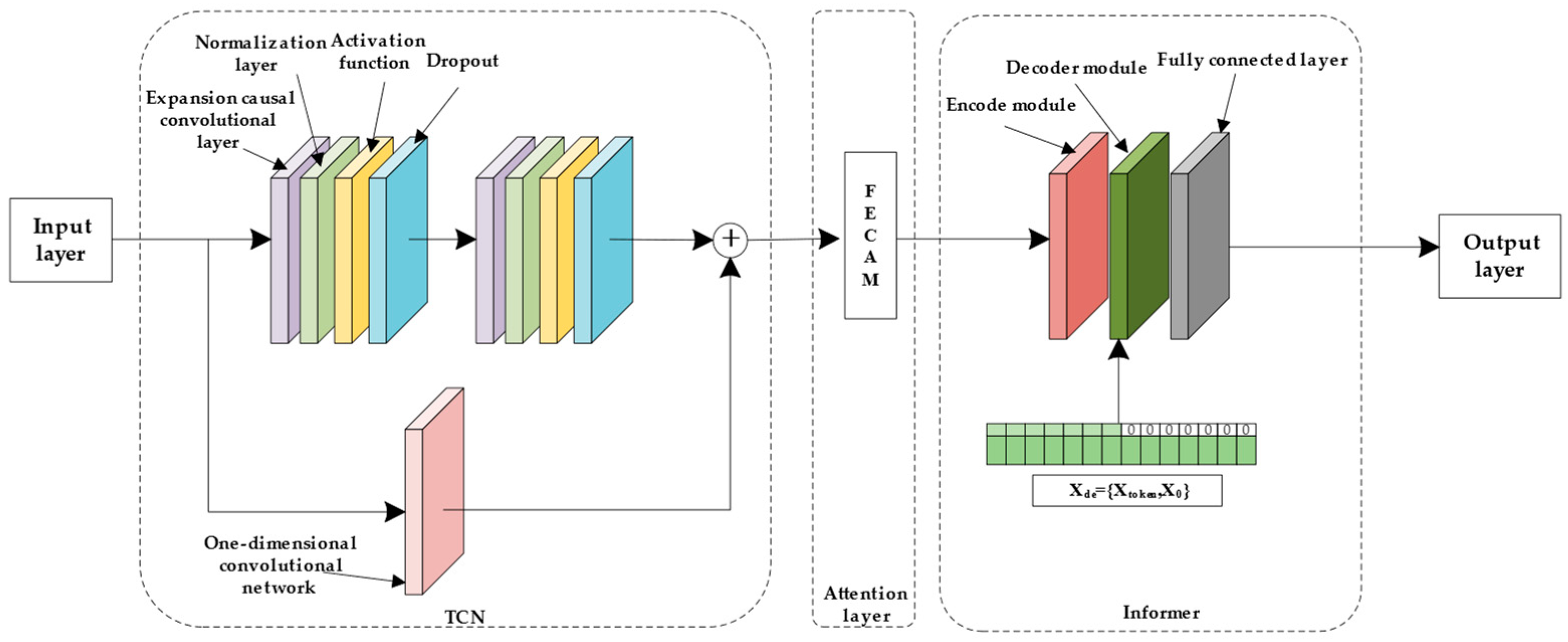
Combined with the analysis of the above-related model structure, this paper proposes a multivariate load pre-model fusing the TCN, frequency-enhanced channel attention mechanism, and Informer network, and it is shown in Figure 2.

Firstly, the features with strong correlation with the load screened by the MIC method are fed into the TCN to extract the local information in it, such as load fluctuation due to rainfall. Secondly, the output of the TCN is processed through the FECAM to enhance the diversity in information of the extracted information, and to generate attention vectors with weights to increase the influence of important features. Then, the processed feature data are input to the Informer network for prediction to obtain the final prediction result.

3. Example Analysis

3.1. Experimental Environment

The experiments in this paper were realized through Python version 3.10.11 with torch version 2.0.1 as the learning framework. The computer configuration was an Intel Core i7-12700H 2.30 GHz CPU, NVIDIA GeForce RTX 3060 laptop GPU (Produced by NVIDIA, a company headquartered in Santa Clara, CA, USA), and a Windows 11 operating system.

3.2. Data Sources

The multivariate load data for the example were the electric, heat, and cold load data from the Tempe School District Integrated Energy System, Tempe, AZ, USA, for the year 2021 [21], and the electric, heat, and cold loads were in kW, MMBTU, and tons, respectively. The meteorological data were the meteorological data from the National Oceanic and Atmospheric Administration website for the year 2021 [22]. The sampling intervals for all the selected data were 1 h, and the data were collected 24 times a day.

3.3. Evaluation Indicators

In this paper, the three parameters of mean absolute error (MAE), root-mean-square error (RMSE), and mean absolute percentage error (MAPE) were selected as the indexes for evaluating the effect of the model. The MAE can be used to identify errors between predictions and actuals, and the RMSE can be used to reflect the degree of deviation between these two. The MAPE can reflect the overall performance of the model. Relevant expressions are shown in

Table 1. Evaluation indicators.

	Definition	Equation
MAE	Mean Absolute Error	$MAE={\displaystyle \frac{1}{m}}{\displaystyle {\sum }_{i=1}^m\left|(Y_i-{\widehat{Y}}_i)\right|}$
RMSE	Root Mean Square Error	$RMSE=\sqrt{{\displaystyle \frac{1}{m}}{\displaystyle {\sum }_{i=1}^m{(Y_i-{\widehat{Y}}_i)}^2}}$
MAPE	Mean Absolute Percentage Error	$MAPE={\displaystyle \frac{100\%}{m}}{\displaystyle \sum _{i=1}^m\left|\frac{{\widehat{Y}}_i-Y_i}{Y_i}\right|}$

$Y_i$ is the true value, ${\widehat{Y}}_i$ is the predicted value, and $m$ is the number of samples in test set.

.

3.4. MIC-Based Feature Correlation Analysis

There are energy conversions between different loads of the IRES and coupling relationships between loads. Therefore, in order to carry out the prediction of multiple IRES loads, the characteristics corresponding to different loads should be clarified first. The characteristics related to different loads are analyzed using MIC analysis, and

Table 2. A correlation analysis of multivariate load and characteristics.

	Electric Load	Heat Load	Cold Load
Temperature	0.43	0.34	0.55
Relative Humidity	0.13	0.11	0.16
Pressure	0.11	0.08	0.14
Wind Speed	0.08	0.05	0.08
Precipitable Water	0.52	0.45	0.53
Surface Reflectance	0.13	0.13	0.17
Electric Load	1	0.50	0.64
Heat Load	0.50	1	0.53
Cold Load	0.64	0.53	1

provides the results.

Firstly, the correlation between multiple loads is analyzed, and the strongest correlation is found between electric and cold load, followed by the correlation between cold and heat load, and the correlation between electric load and heat load, which are 0.53 and 0.5, respectively. Then, the meteorological correlation characteristics are analyzed. Electric, heat, and cold load are all strongly correlated with temperature and precipitable water, while the correlations with the other features are weak. In conclusion, there are both strong and relatively weak correlations between multiple loads, and temperature and precipitable water among meteorological factors are the key features affecting multiple loads. Therefore, the multivariate loads and the key features selected are shown in Figure 3.

3.5. Comparative Analysis of Forecast Results

3.5.1. Comparison of Multiple Load Forecasting and Single Load Forecasting

In order to verify the effectiveness of the MIC method in multivariate load forecasting and the difference in the strength of the correlation between multivariate loads and multiple factors, single load forecasting and multivariate load forecasting are compared, and the results are shown in

Table 3. Single load forecasting and multivariate load forecasting results.

	MAPE/%
	Electric Load	Heat Load	Cold Load
Single load forecasting	2.98	3.80	7.92
Multiple load forecasting	2.25	3.69	10.21

.

The multivariate load prediction considers the mutual coupling characteristics among electric, heat, and cold loads, which reduces the errors of electric, heat, and cold loads by 24.5%, 2.90%, and 22.42%, respectively, indicating that there is a correlation among the multivariate loads. In the comprehensive energy system of the campus, the correlation between electric load, cooling load, and other loads is strong, and the correlation between heat load and other loads is weak.

3.5.2. Results of Different Model Predictions

To verify the validity of the proposed model, the results of multivariate load forecasting of this paper’s model is compared with those of TCN-Informer, Informer, and TCN-FECAM-Transformer. The learning rate of the proposed model is set to 0.0001, the step size is set to 30, the batch size is set to 32, and the number of training iterations is 60.

(1)

Comparison of TCN-FECAM-Informer, TCN-Informer, and Informer

By comparing this paper’s model TCN-FECAM-Informer with TCN-Informer and the Informer model in electric, heat, and cold multivariate load forecasting, the evaluation results of individual models are obtained to verify the performance of this paper’s model, and the results are shown in

Table 4. Comparison of TCN-FECAM-Informer, TCN-Informer, and Informer in electric load forecasting.

	Electric Load/kW
	MAPE/%	MAE	RMSE
Informer	2.64	405.56	583.27
TCN-Informer	1.76	264.08	368.45
TCN-FECAM-Informer	1.36	205.01	287.46

,

Table 5. Comparison of TCN-FECAM-Informer, TCN-Informer, and Informer in heat load forecasting.

	Heat Load/MMBTU
	MAPE/%	MAE	RMSE
Informer	4.27	74.56	96.88
TCN-Informer	2.96	51.70	65.03
TCN-FECAM-Informer	2.03	35.21	45.10

and

Table 6. Comparison of TCN-FECAM-Informer, TCN-Informer, and Informer in cold load forecasting.

	Cold Load/Tons
	MAPE/%	MAE	RMSE
Informer	4.91	688.43	918.01
TCN-Informer	4.57	609.26	814.59
TCN-FECAM-Informer	4.00	545.49	730.27

below.

Analyzing the prediction results, the following conclusions can be drawn: firstly, in multivariate load prediction, the prediction error of the TCN-Informer network is lower than that of the Informer model, which indicates that the TCN is able to carry out preliminary extraction of the local features of the factors affecting the load, and thus the overall prediction effect of the combined model is superior to that of the single network model. In contrast, the model proposed in this paper combines the FECAM to analyze the frequency domain of the processed data from TCNs, filtering the high-frequency noise to further enhance the effectiveness of the extracted features, which further improves the effectiveness in dealing with multivariate load forecasting. The prediction error of the TCN-FECAM-Informer model is lower than that of the TCN-Informer model, in which the MAPE of the electric, heat, and cooling loads decreases by 22.7%, 31.4%, and 12.5%, respectively. In summary, the combined forecasting model proposed in this paper has good forecasting results and is feasible in multivariate load forecasting. The multivariate load forecasting results of different models are shown in Figure 4, Figure 5 and Figure 6 below.

(2)

Comparison between TCN-FECAM-Informer, TCN-FECAM-Transformer, and LSTM

In order to analyze the impact of the underlying network choice on the model prediction performance, this paper compares the proposed model with the TCN-FECAM-Transformer model and the LSTM model, which is a network that uses LSTM for both the encoder and decoder. The results are shown in

Table 7. Comparison of TCN-FECAM-Informer, TCN-FECAM-Transformer, and LSTM in electric load forecasting.

	Electric Load/kW
	MAPE/%	MAE	RMSE
LSTM(Seq2seq)	5.10	750.99	1006.56
TCN-FECAM-Transformer	2.26	319.77	400.34
TCN-FECAM-Informer	1.36	205.01	287.46

,

Table 8. Comparison of TCN-FECAM-Informer, TCN-FECAM-Transformer, and LSTM in heat load forecasting.

	Heat Load/MMBTU
	MAPE/%	MAE	RMSE
LSTM(Seq2seq)	8.80	145.01	178.03
TCN-FECAM-Transformer	3.69	65.27	83.42
TCN-FECAM-Informer	2.03	35.21	45.10

and

Table 9. Comparison of TCN-FECAM-Informer, TCN-FECAM-Transformer, and LSTM in cold load forecasting.

	Cold Load/Tons
	MAPE/%	MAE	RMSE
LSTM(Seq2seq)	29.90	3639.03	3984.12
TCN-FECAM-Transformer	7.93	966.05	1175.56
TCN-FECAM-Informer	4.00	545.49	730.27

.

The prediction effect of the LSTM model is not as good as those of the other two models. The transformer model and Informer model are encoder–decoder architecture models based on the attention mechanism, which are unsupervised learning models. In this paper, supervised training is used for training, and the attention mechanisms of the transformer network and Informer network are utilized to calculate the correlation between the data at any position of the input sequence, to explore more effective information of the input sequence, to overcome the problem of long dependence on the data that cannot be extracted by the traditional recurrent neural network, and to improve the overall prediction performance of the model. The Informer network, on the other hand, improves on the transformer network and further enhances the predictive performance of the model, with the MAPE of electric, heat, and cold loads reduced by 39.8%, 45.0%, and 49.6%, respectively. The comparison results are shown in Figure 7, Figure 8 and Figure 9 below.

4. Conclusions

In this paper, in order to deal with the coupling relationship between multivariate loads for IRESs, which include low-carbon-emission renewable energy sources, the correlation analysis and feature selection of different influencing factors of multivariate loads are carried out by using the MIC; the basic principles of the FECAM, TCN, and Informer network are analyzed; and the TCN-FECAM-Informer multivariate load forecasting model is proposed.

The TCN-FECAM-Informer multivariate load combination prediction model proposed in this paper gives full play to the feature information extraction capability of the TCN, FECAM, and Informer network, thus improving the prediction accuracy of multivariate loads, which has certain application prospects in the field of multivariate load prediction and provides ideas for the subsequent research.

In future research, methods to enhance the performance of IRES multivariate load forecasting under more uncertainties will be further analyzed.

References

1. Jin, Y.; Xiong, X.; Zhang, J.; Pan, L.; Li, Y.; Wu, X.; Shen, J. A prospective review on the design and operation of integrated energy system: The spotlight cast on dynamic characteristics. Appl. Therm. Eng. 2024, 253, 123751. [Google Scholar] [CrossRef]
2. Tan, Z.; De, G.; Li, M.; Lin, H.; Yang, S.; Huang, L.; Tan, Q. Combined electricity-heat-cooling-gas load forecasting model for integrated energy system based on multi-task learning and least square support vector machine. J. Clean. Prod. 2020, 248, 119252. [Google Scholar] [CrossRef]
3. Li, G.; Li, Y.; Roozitalab, F. Midterm Load Forecasting: A Multistep Approach Based on Phase Space Reconstruction and Support Vector Machine. IEEE Syst. J. 2020, 14, 4967–4977. [Google Scholar] [CrossRef]
4. Madhukumar, M.; Sebastian, A.; Liang, X.; Jamil, M.; Shabbir, M.N.S.K. Regression Model-Based Short-Term Load Forecasting for University Campus Load. IEEE Access 2022, 10, 8891–8905. [Google Scholar] [CrossRef]
5. Zhao, P.; Cao, D.; Hu, W.; Huang, Y.; Hao, M.; Huang, Q.; Chen, Z. Geometric Loss-Enabled Complex Neural Network for Multi-Energy Load Forecasting in Integrated Energy Systems. IEEE Trans. Power Syst. 2024, 39, 5659–5671. [Google Scholar] [CrossRef]
6. Wang, Y.; Wang, H.; Meng, X.; Dong, H.; Chen, X.; Xiang, H.; Xing, J. Considering the dual endogenous-exogenous uncertainty integrated energy multiple load short-term forecast. Energy 2023, 285, 129387. [Google Scholar] [CrossRef]
7. Hu, J.; Hu, W.; Cao, D.; Sun, X.; Chen, J.; Huang, Y.; Chen, Z.; Blaabjerg, F. Probabilistic net load forecasting based on transformer network and Gaussian process-enabled residual modeling learning method. Renew. Energy 2024, 225, 120253. [Google Scholar] [CrossRef]
8. Xu, P.; Song, Y.; Du, J.; Zhang, F. Town gas daily load forecasting based on machine learning combinatorial algorithms: A case study in North China. Chin. J. Chem. Eng. 2024, in press. [CrossRef]
9. Shi, J.; Teh, J.; Alharbi, B.; Lai, C.-M. Load forecasting for regional integrated energy system based on two-phase decomposition and mixture prediction model. Energy 2024, 297, 131236. [Google Scholar] [CrossRef]
10. Yang, Y.; Wang, Z.; Zhao, S.; Wu, J. An integrated federated learning algorithm for short-term load forecasting. Electr. Power Syst. Res. 2023, 214, 108830. [Google Scholar] [CrossRef]
11. Chen, J.; Hu, Z.; Chen, W.; Gao, M.; Du, Y.; Lin, M. Load prediction of integrated energy system based on combination of quadratic modal decomposition and deep bidirectional long short-term memory and multiple linear regression. Autom. Electr. Power Syst. 2021, 45, 85–94. [Google Scholar]
12. Chen, H.; Huang, H.; Zheng, Y.; Yang, B. A load forecasting approach for integrated energy systems based on aggregation hybrid modal decomposition and combined model. Appl. Energy 2024, 375, 124166. [Google Scholar] [CrossRef]
13. Zhang, Y.; Sun, M.; Ji, X.; Ye, P.; Yang, M.; Cai, F. Short-term load forecasting of integrated energy system based on modal decomposition and multi-task learning model. High Volt. Eng. 2024, 1–18. [Google Scholar] [CrossRef]
14. Xuan, W.; Shouxiang, W.; Qianyu, Z.; Shaomin, W.; Liwei, F. A multi-energy load prediction model based on deep multi-task learning and ensemble approach for regional integrated energy systems. Int. J. Electr. Power Energy Syst. 2021, 126, 106583. [Google Scholar] [CrossRef]
15. Li, R.; Sun, F.; Ding, X.; Han, Y.; Liu, Y.; Yan, J. Ultra-short-term load forecasting method of user-level integrated energy system considering multi-energy space-time coupling. Power Syst. Technol. 2020, 44, 4121–4131. [Google Scholar]
16. Tian, Z.; Liu, W.; Jiang, W.; Wu, C. CNNs-Transformer based day-ahead probabilistic load forecasting for weekends with limited data availability. Energy 2024, 293, 130666. [Google Scholar] [CrossRef]
17. Limouni, T.; Yaagoubi, R.; Bouziane, K.; Guissi, K.; Baali, E.H. Accurate one step and multistep forecasting of very short-term PV power using LSTM-TCN model. Renew. Energy 2023, 205, 1010–1024. [Google Scholar] [CrossRef]
18. Wu, X.; Fan, B.; Wang, J.; Hu, Q. Life prediction of lithium battery based on VMD-TCN-Attention. Chin. J. Power Sources 2023, 47, 1319–1325. [Google Scholar]
19. Hu, J.; Shen, L.; Sun, G. Squeeze-and-Excitation Networks. In Proceedings of the 2018 IEEE/CVF Conference on Computer Vision and Pattern Recognition, Salt Lake City, UT, USA, 18–23 June 2018; pp. 7132–7141. [Google Scholar]
20. Jiang, M.; Zeng, P.; Wang, K.; Liu, H.; Chen, W.; Liu, H. FECAM: Frequency enhanced channel attention mechanism for time series forecasting. Adv. Eng. Inform. 2023, 58, 102158. [Google Scholar] [CrossRef]
21. Aus. Campus Metabolism [DB/OL] America. Available online: http://cm.asu.edu/ (accessed on 31 July 2023).
22. National Centers for Environmental Information [DB/OL] America. Available online: https://www.ncei.noaa.gov/ (accessed on 31 July 2023).
Figure 1. Residual connectivity module structure.
Energies 17 05181 g001
Figure 2. The whole framework of TCN-FECAM-Informer.
Energies 17 05181 g002
Figure 3. Characterization of the main effects of multiple loads.
Energies 17 05181 g003
Figure 4. Comparison of TCN-FECAM-Informer, TCN-Informer, and Informer in electric load forecasting.
Energies 17 05181 g004
Figure 5. Comparison of TCN-FECAM-Informer, TCN-Informer, and Informer in heat load forecasting.
Energies 17 05181 g005
Figure 6. Comparison of TCN-FECAM-Informer, TCN-Informer, and Informer in cold load forecasting.
Energies 17 05181 g006
Figure 7. Comparison of TCN-FECAM-Informer, TCN-FECAM-Transformer, and LSTM in electric load forecasting.
Energies 17 05181 g007
Figure 8. Comparison of TCN-FECAM-Informer, TCN-FECAM-Transformer, and LSTM in heat load forecasting.
Energies 17 05181 g008
Figure 9. Comparison of TCN-FECAM-Informer, TCN-FECAM-Transformer, and LSTM in cold load forecasting.
Energies 17 05181 g009