Fusion Forecasting Algorithm for Short-Term Load in Power System

Abstract

Short-term load forecasting plays an important role in power system scheduling, optimization, and maintenance, but no existing typical method can consistently maintain high prediction accuracy. Hence, fusing different complementary methods is increasingly focused on. To improve forecasting accuracy and stability, these features that affect the short-term power system are firstly extracted as prior knowledge, and the advantages and disadvantages of existing methods are analyzed. Then, three typically methods are used for short-term power load forecasting, and their interaction and complementarity are studied. Finally, the Choquet integral (CI) is used to fuse the three existing complementarity methods. Different from other fusion methods, the CI can fully utilize the interactions and complementarity among different methods to achieve consistent forecasting results, and reduce the disadvantages of a single forecasting method. Essentially, a CI with n inputs is equivalent to n! constrained feedforward neural networks, leading to a strong generalization ability in the load prediction process. Consequently, the CI-based method provides an effective way for the fusion forecasting of short-term load in power systems.

1. Introduction

Short-term load forecasting is a crucial task in the power system and serves as a fundamental basis for power load scheduling, optimization, and maintenance [1]. However, the power loads have real-time, rapid-changeable, and non-storage characteristics. Ensuring the stability, safety, and economy of the power system through accurate forecasting has always been a key issue [2].

The current effective forecasting methods include two categories [3], current deep learning and traditional machine learning. The deep learning methods that have been applied to short-term load forecasting in power systems include convolutional neural networks, long short-term memory networks, and lightweight networks, etc. [4]. Deep learning methods can effectively solve load forecasting issues if there are sufficient representative samples and if load changes exhibit a strong repeatability. However, for short-term power system load forecasting, the above conditions often are not met, and thus their predicted results may have a high uncertainty and produce significant errors [5]. Moreover, their interpretability and operability are often quite restricted. On the other hand, traditional machine learning methods are effective under certain conditions and usage environments. Notably, three commonly used algorithms are Kalman filtering (KF) [6], backpropagation (BP) neural networks [7], and the gray system (GS) model [8], each with its own characteristics and applicable range. These methods have the advantages of clear principles, easy realization, and good interpretability.

KF is a recursive, optimally filtering and forecasting method. It is a highly efficient and useful method for solving a large amount of time series forecasting problems with prior and subsequent correlations. When KF is used for power system load forecasting, it may have an easy realization, clear principles, and stable forecasting results. However, KF is easily affected by noise and nonlinear variables [9]. For irregular load changes, constructing the recursive matrix and observation matrix in KF is key and challenging in practice. Moreover, possible random interference factors and noisy data also limit its forecasting accuracy and stability.

The BP neural network is widely used in traditional machine learning, with numerous open-source systems and functional modules available in most software packages and computing platforms. The use of BP for short-term load forecasting can establish causal relationships between various related factors, offer explanations for load measurements, and improve forecasting accuracy under certain conditions. However, BP networks have evident limitations, such as the difficulty in avoiding the problem of local optima of the objective function and the gradient disappearing in the learning process [10], which have not been fundamentally solved so far.

The GS is a modeling and approximation method based on gray theory [11]. It is a simple and practical method to solve modeling, forecasting, and optimization in inconsistent, uncertain, and incomplete situations. Currently, many uncertain and random factors affect daily power load changes, and both mechanistic and semi-mechanistic models struggle to accurately describe and quantitatively calculate these factors. In contrast, the GS method offers advantages such as simple calculations, strong practicality, and a high accuracy for power forecasting, particularly when the load changes are not rapid. So, the GS may be suitable for short-, mid-, and long- term power load forecasting. However, GS-based forecasting is less effective when samples are complex. Especially for time series with long-term and persistent load changes, the forecasting results may be inaccurate.

In summary, the above studies partially or entirely use meteorological information, daily patterns, and historical loads as the key factors of feature selection in the forecasting of power load [12]. Their input features are not processed based on the characteristics of the short-term load forecasting task before inputting the features into the forecasting model, optimization, and computation. Therefore, they are unable to effectively utilize existing experience and prior knowledge in the learning and forecasting models. Furthermore, most machine learning-based methods the predict power load independently and do not consider integration and time series characteristics, leading to limitations such as a reduced applicability and unstable results [13]. Nevertheless, integrating multiple load forecasting methods can provide more accurate and stable short-term forecasting for the power system, offering practical significance and urgency.

In this study, the three commonly used short-term load forecasting methods, KF, BP, and GS, are used to model and predict short-term loads. After exploring their applicability and complementarity, the Choquet integral (CI) model [14] is proposed as a fusion forecasting method to enhance accuracy and stability. The CI is a nonlinear fusion model that considers the interactions among various methods or information sources. It can automatically identify the advantages and disadvantages of different methods by solving model parameters, and thereby endowing a higher importance to those accurate sources, reducing the limitations of single methods in predicting unstable or inaccurate results under different conditions. The proposed method based on the CI is validated by predicting the annual load data of a certain district in Tianjin, China, and further practical results are obtained as to the applicability of the new method.

2. Related Work

2.1. KF Technique

The KF provides the state estimation of any dynamic system through recursive relationships, and is the optimal estimator for non-stationary stochastic processes under the criterion of minimum error covariance [15]. The implementation of KF consists of the following five fundamental equations [16]:

$$Y_k=H_k{X}_k+W_k (\mathrm{Measurement} \mathrm{equation})$$

(1)

$$X_{k+1}=A_k{X}_k+V_k (\mathrm{State} \mathrm{equation})$$

(2)

where $A_k$ is the one-step state transition matrix; $V_k$ is the dynamic noise of the system at the kth moment; $H_k$ is the observation matrix; $X_k$ is an N-dimensional state vector; and $W_k$ is the random interference noise at the kth moment. The forecasting at time (k + 1) is

$${\tilde{X}}_{k+1}=A_k{\widehat{X}}_k$$

(3)

where ${\widehat{X}}_k$ is the filtering estimation at time k. After obtaining the new measurement Y_k+1, the forecasting error $(Y_{k+1}-{\tilde{Y}}_{k+1})$ is multiplied by an appropriate coefficient as the correction term for state forecasting, and the estimated value at time k + 1 is obtained as

$${\tilde{X}}_{k+1}=A_k{\widehat{X}}_k+K_{k+1}(Y_{k+1}-H_{k+1}{A}_k{\widehat{X}}_k)$$

(4)

After selecting the gain matrix $K_{k+1}$, the covariance matrix of the estimation error $(X_{k+1}-{\widehat{X}}_{k+1})$ is obtained as

$$P_{k+1}=E\{(X_{k+1}-{\widehat{X}}_{k+1}){(X_{k+1}-{\widehat{X}}_{k+1})}^T\}$$

(5)

The KF forecasting result is achieved by recursively using the above five key equations.

2.2. BP Neural Network

BP first selects the factors that primarily reflect load changes as the input X of the network and uses the load forecasting value Y as the output. This forms a pair (X, Y) and further constructs a time series. The BP modeling steps are as follows [17]:

Step 1. Initialize parameters. Namely, the number of input layer nodes n, the number of hidden layer nodes l, the number of output layer nodes m, the connection weights W_ij and W_jk from the input to the hidden layer and output layer neurons, the hidden layer threshold a, the output layer threshold b, and learning rate $\eta$.

Step 2. Compute hidden layer. The output in the hidden layer H_j is calculated as

$$H_j=f({\displaystyle {\sum }_{i=1}^n{W}_{ij}}{X}_i-a),i=1,2,\dots ,n;j=1,2,\dots ,l$$

(6)

where f is the hidden layer excitation function.

Step 3. Update output. It is calculated as

$$O_k={\displaystyle {\sum }_{j=1}^i{H}_j{W}_{jk}-b_k},k=1,2,\dots ,m$$

(7)

Step 4. Calculate error. According to O_k and the actual/real output Y_k, the error e_k is calculated as

$$e_k=Y_k-O_k,k=1,2,\dots ,m$$

(8)

Step 5. Update weighting value. The connecting weighting values among the nodes are calculated as

$$W_{ij}=W_{ij}+\eta H_j(1-H_j)X_i{\displaystyle {\sum }_{k=1}^m{W}_{jk}}{e}_{k}s.t., W_{jk}=W_{jk}+\eta H_j{e}_k$$

(9)

where i = 1, …, n; j = 1, …, l; k = 1, …, m.

Step 6. Update threshold. The threshold is updated as

$$\left\{\begin{array}{l}{a}_j=a_j+\eta H_j(1-H_j){\displaystyle {\sum }_{k=1}^m{W}_{jk}}{e}_k,j=1,2,\dots ,l\\ b_j=b_k+e_k,k=1,2,\dots ,m\end{array}\right.$$

(10)

2.3. GS Model

The GS model uses any historical data series to establish a differential equation as

$$dX/dt+aX=u$$

(11)

where a and u are a pair of coefficients [18].

Let the variable X⁽⁰⁾ be the original data sequence X⁽⁰⁾ = (X⁽⁰⁾(1), X⁽⁰⁾(2), …, X⁽⁰⁾(n)) that generates the following first-order sequence as

$$X^{(1)}=(X^{(1)}(1),X^{(1)}(2),\dots ,X^{(1)}(n)), s.t., X^{(1)}\left(k\right)={\displaystyle {\sum }_{i=1}^k{x}^{(0)}(i)}$$

(12)

where X⁽¹⁾(k) satisfies the discrete form along the following differential equations,

$$X^{(1)}(k+1)=[X^{(0)}(1)-\widehat{u}/\widehat{a}]e^{\widehat{a}k}+\widehat{u}/\widehat{a}$$

(13)

The GS model for the original data column X⁽⁰⁾ can be obtained by

$${\widehat{X}}^{(0)}(k+1)={\widehat{X}}^{(1)}(k+1)-{\widehat{X}}^{(1)}(k)=(e^{-a}-1)[X^{(0)}(1)-\widehat{u}/\widehat{a}]e^{\widehat{a}k}$$

(14)

where k = 0, 1, 2, 3, …

In the GS model, the sequence X⁽¹⁾(k) obeys an exponential growth law, and its solution follows the discrete first-order differential equation as

$$X^{(1)}(k+1)+{\displaystyle \frac{1}{2}}a[X^{(1)}(k+1)+X^{(1)}(k)]=u, k=1,2,\dots ,n$$

(15)

Based on the residual between the predicted and the actual value, the least squares criteria method can estimate the values of a and u. Hence, the power load forecasting can be realized by (15).

3. Proposed Fusion Method

3.1. Feature Extraction

The total load of the power system L can generally be decomposed into four components according to the type of influencing factors [19], namely

L = L_n + L_w + L_s + L_r

(16)

where L_n represents the normal trend of the load component, typically characterized by the load of typical historical days; L_w is the power load component related to meteorological factors, primarily influenced by changes in various meteorological factors; L_s is caused by special external factors such as holidays; and L_r is a random component of the power load, which, while having a small proportion, is usually difficult to predict. Therefore, we focus on the first three key factors.

(1) Temperature and humidity: Based on previous research experiences in power load forecasting [20], the two meteorological factors of temperature and relative humidity have the strongest correlation with power system load. Thus, we construct their daily mean and variance into a vector,

H_k = (t_m(k), t_v(k), h_m(k), h_v(k)), k = 1, 2, …, K,

(17)

where K is the total number of observed days, and t_m(k) and t_v(k) refer to the daily mean and variance of the temperature_, and h_m(k) and h_v(k) those of the humidity. According to the range of annual temperature and humidity in the detection area, the ranges of the four variables can be determined. All the above vectors consist of a set SH = {H_k|k = 1, 2, …, K}.

(2) Special days. The power loads are very different between working and non-working days, and particularly special days such as Spring Festival, Labor Day, and National Day. Each of them usually includes a group of continuous non-working days. Hence, a feature vector to represent any special day is constructed as follows,

D_q = (d_q1, d_q2,⋯, d_qm), q = 1, 2,…,Q;

(18)

where q denotes the qth special day, m is the number of non-working days, and Q is the total number of special days. All such vectors consist of a set, SD = {D_q|q = 1, 2, …, Q}.

(3) Normal day. Owing to the cyclical and continuous changes, normal historical power loads from a week except special days are nearly repeated [21]. Assume that the total number of normal days is N; all normal days consist of a set, SN = {D_p|p = 1, 2, …, N}.

Therefore, the power load must be forecasted individually over special days and normal days after considering the influences of temperature and humidity. And any predicted power load firstly is distinguished by SD∪SH with relative power loads, and SN∪SH with relative power loads, respectively.

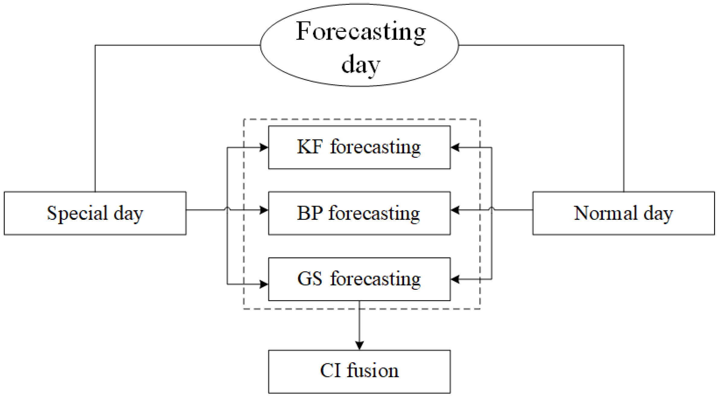
Let the forecasting model be q = F(H, c), where q is the power load and c is the data type. We use KF, BP, and the GS to construct forecasting models to approximate F(·,·) using historical data. For each predicted day, the three models provide power load forecastings, which are then integrated into the CI model to achieve a more accurate forecasting of power loads. Figure 1 shows the flowchart of our proposed model.

3.2. Forecasting of the Three Existing Typical Methods

As an example, the historical load data used in this study consists of daily 24 h loads in a district in Tianjin from 1 July 2019 to 30 June 2021. The sampling unit is hours, and in total, 17,088 pieces of data are collected.

Table 1. Data features of historical loads in two years (unit: MW).

Period\Feature	Maximum	Minimum	Average	Variance	Standard Deviation
June 2019–June 2020	4785.15	1834.64	3206.40	789.93	28.11
July 2020–July 2021	3464.79	587.22	2345.73	312.54	17.68

shows their main features, such as their maximum, minimum, average, standard deviation, and variance. All data are partitioned into two groups, and the data in the first year are used to construct the forecasting model and the second year to evaluate the predicting accuracy of the model.

3.2.1. KF Forecasting

The KF forecasting method is developed using relative power loads from SD∪SH and SN∪SH in the first year. Denote the load data at time k as q_k, k = 1, 2, …, n. Each piece of data is defined as a node, and the kth node refers to a three-dimensional vector $X_k:(q_k,q_k^{\prime },q_k^{″})$, where $q_k^{\prime }$ and $q_k^{″}$ are defined as

$$q_k^{\prime }=q_k-q_{k-1} and q_k^{″}=q_k^{\prime }-q_{k-1}^{\prime }$$

(19)

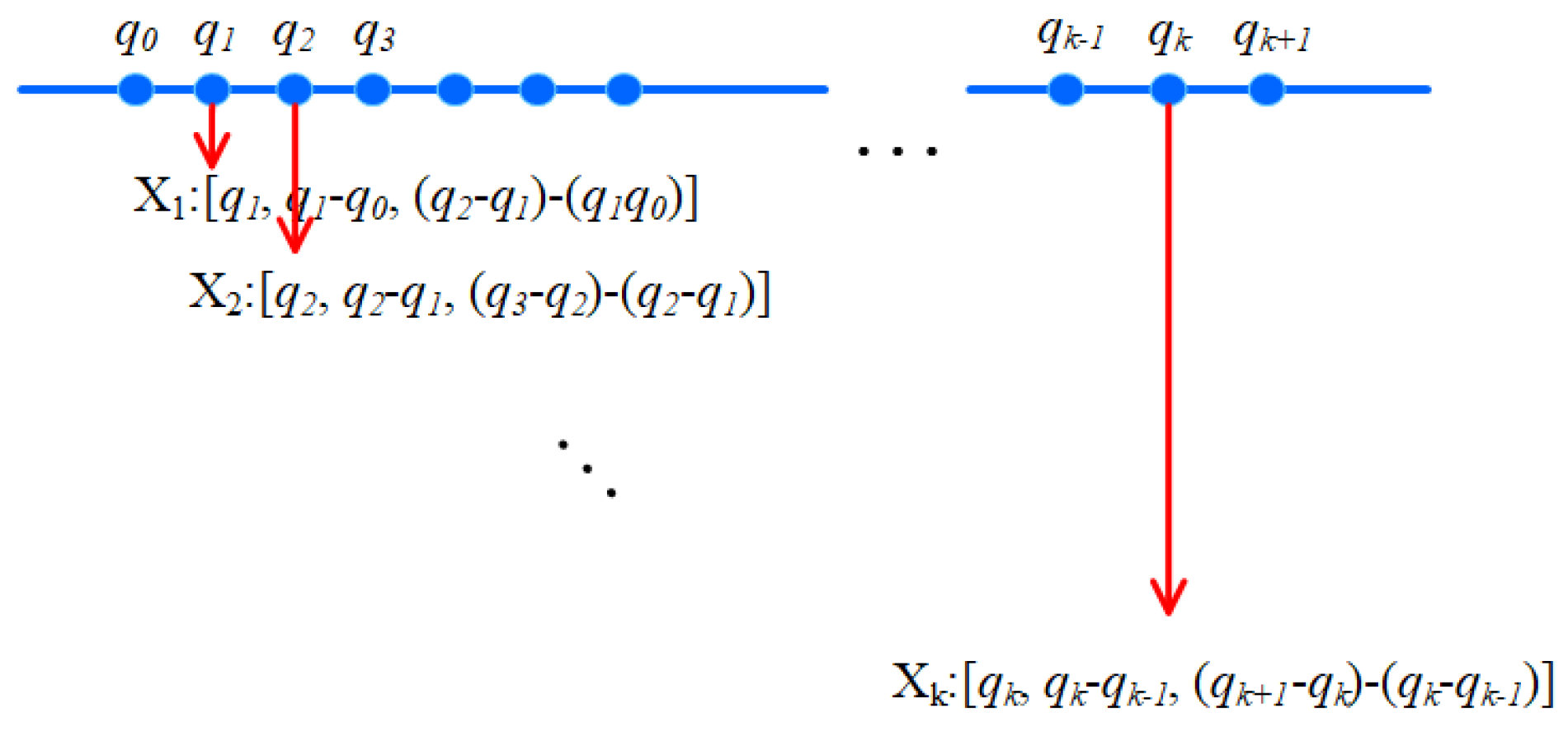
They are the first-order and the second-order differences of q_k, and are recursively computed. The calculation process is shown in Figure 2.

After recording the load every day along each regular interval (1 h), 24 daily sampling values are obtained, and the three-dimensional representation of the measurement nodes can be obtained, $X_t(q_t,q_k^{\prime },q_k^{″})$. Hence, the KF matrix coefficient A is determined as follows. Since

$$q_k^{\prime }=q_{k-1}^{\prime }+q_{k-1}^{″} and q_k=q_{k-1}+q_{k-1}^{\prime }+q_{k-1}^{″}$$

(20)

the coefficient matrix A in the KF equation is obtained as

$$\left[\begin{array}{l}{q}_k\\ q_k^{\prime }\\ q_k^{″}\end{array}\right]=A\left[\begin{array}{l}{q}_{k-1}\\ q_{k-1}^{\prime }\\ q_{k-1}^{″}\end{array}\right]=\left[\begin{array}{l}1 1 1\\ 0 1 1\\ a b c\end{array}\right]\left[\begin{array}{l}{q}_{k-1}\\ q_{k-1}^{\prime }\\ q_{k-1}^{″}\end{array}\right]$$

(21)

When there is no other available prior information, the measurement matrix H_k is taken as the identity matrix.

Using the following seven special days, such as New Year’s Day, Spring Festival, Tomb-Sweeping Day, Labor Day, the Long Boat Festival, Mid-Autumn Festival, and National Day, as dividing points, we divide the entire year from June 2019 to June 2020 into 7 stages to determine the parameters in each forecasting model. In the same way, the year from July 2020 to July 2021 is divided into 7 stages for load forecasting. In every stage, the forecasting is performed in every hour of all days. The KF forecasting accuracy is evaluated by a group of statistical quantities in each stage, such as maximal absolute error, average absolute relative error, average relative error, and standard error, as shown in

Table 2. KF forecasting error for 7 stages (unit: MW).

Stage	Maximal Absolute Error	Average Absolute Error	Average Relative Error	Standard Error
1	685.982	486.239	29.7%	166.267
2	64.010	43.845	18.0%	12.137
3	550.280	467.083	25.3%	82.295
4	321.439	224.451	24.3%	49.528
5	436.222	253.580	37.6%	69.458
6	441.775	310.238	38.6%	73.582
7	358.751	198.239	15.6%	70.223

as follows.

The following conclusions can be inferred from Table 2.

(1) The minimum forecasting error occurs in the second stage, but the forecasting error tends to stabilize from the third stage onwards. This is because the KF method is advantageous as it is an adaptive process with a dynamic correction function. It updates the state variables using the estimated value from the previous moment and the observed value at the current moment to obtain the estimated value at this stage.

(2) The maximum absolute error ranges from 64.010 to 685.982 MW, the average absolute error ranges from 43.845 to 486.239 MW, the average relative error ranges from 15.6% to 38.6%, and the standard deviation ranges from 12.137 to 166.267, respectively. All error indicators are relatively high. This is because the parameters of the KF model significantly impact the forecasting results, with the state transition matrix having a particularly notable effect on the KF forecasting. Especially in the KF forecasting process, the state matrix is inferred based on the load information of the first two months of every two quarters, and its accuracy directly affects the forecasting results.

(3) Analysis of the measurement period reveals that the average relative error of load forecasting change during the National Day Golden Week is the smallest. Load value fluctuations are relatively small in summer and winter, while they are larger in spring and autumn. This indicates that seasonal variations impact the accuracy of the forecasting results.

3.2.2. BP Forecasting

The process of solving the BP network model is as follows:

(1)

Input and output layer design: The inputs of the BP take the first-order and second-order difference of hourly loads, and the output is the load. Therefore, the number of nodes in the input layer is 2, and that in the output layer is 1.

(2)

Hidden layer design: We use a multi-input–single-output BP network with three hidden layers for load forecasting. The determination of the number of hidden layer neurons is very important, and we thus refer to the empirical formula [22]:

$$l=\sqrt{n+m}+a$$

(22)

where n is the number of input layer neurons, m is the number of output layer neurons, and a is a constant between the range [1, 10]. Therefore, the number of neurons in the BP network in each quarter can be calculated.

(3)

Selection of incentive function: There are various transfer functions for BP neural networks. But with periodic data, using the tansig function for the transfer function has smaller errors and higher stability than the logsig function. Therefore, tansig is used, and the Purelin function is used as the transfer function in the output layer.

(4)

Network parameter determination: Let the network parameters have 5000 epochs of network iterations and an expected error of 10⁻⁵. The forecasting model established in the first two months of each quarter forecasts the third month by the BP neural network method; the experimental results are shown in

Table 3. Analysis of forecasting results using BP neural network (unit: MW).

Stage	Maximal Absolute Error	Average Absolute Error	Average Relative Error	Standard Error
1	33.545	26.783	3.8%	14.948
2	26.871	20.127	9.7%	4.092
3	466.754	354.853	13.9%	70.371
4	83.295	50.385	10.0%	31.331
5	134.968	100.358	13.1%	49.695
6	129.702	87.453	11.2%	54.244
7	136.513	89.729	23.4%	49.288

.

The results can be inferred from Table 3 as follows.

(1) In some stages, there are individual points in the predicted results with significant forecasting errors, and some forecasting values deviate from the actual values. This may be due to the inherent drawback of local extremum points in the BP algorithm.

(2) The maximum absolute error is between 26.871 and 466.754 MW, the average absolute error ranges from 20.127 to 354.853 MW, the average relative error is between 3.8% and 23.4%, and the standard deviation is between 4.092 and 70.371.

(3) In the forecasting results of each quarter, the absolute and relative errors of the first, second, and fourth stages are relatively small, while the errors of other stages are relatively large, indicating that different stages each day have a certain impact on the accuracy.

3.2.3. GS Forecasting

When using the GS, both parameters a and u must be determined. We determined them through fitting the samples in the year from June 2019 to June 2020, as shown in

Table 4. GS parameters of four quarters.

Quarter	1	2	3	4
a	0.954	0.813	0.762	0.742
u	0.322	0.455	0.651	0.658

.

After taking these parameters into (13),

Table 5. The GS forecasting results (unit: MW).

Stage	Maximal Absolute Error	Average Absolute Error	Average Relative Error	Standard Error
1	26.566	18.732	3.2%	9.478
2	6.932	5.054	1.6%	1.178
3	109.351	87.239	17.1%	6.631
4	68.195	50.780	16.0%	3.452
5	97.388	83.227	12.5%	43.597
6	89.640	50.718	11.8%	41.034
7	81.050	65.450	18.5%	8.787

shows the errors in all seven stages.

The following results can be inferred from Table 5.

(1) The maximum absolute error predicted by the GS model is between 6.9329 and 109.3515 MW, the average absolute error ranges from 5.054 to 87.239 MW, the average relative error is between 1.62% and 18.57%, and the standard deviation is between 1.1782 and 43.5972. After evaluating these data, it was found that the GS forecasting results did not fluctuate up and down with the actual load value. The overall predicted trend manifests as exponential characteristics, which should be consistent with the actual situation in the short term. However, the general future load trend will not fully obey the exponential growth characteristics, which is the reason that the GS generates the larger error.

(2) The maximum absolute error, average relative error, and standard deviation of the predicted results outside the third and fifth stages are relatively small; especially, the absolute error of the forecasting in the second stage reaches small values, basically reaching the small error level that can be used for load forecasting. However, the GS has certain limitations and is only suitable for modeling and forecasting problems with relatively gentle data changes. It is not suitable for situations where the growth rate of data sequences is too fast or exhibits significant fluctuations.

3.3. Fusion Based on CI Model

Let X = {x₁, x₂, …, x_n} be a set of n inputs (components) and P(X) be the power set of X. The set function g on X: P(X)→[0, 1] is called a non-additive measure [23], which represents the interrelation among the n inputs, satisfying

(1)

Boundary condition: $g(\varphi )=0,g(X)=1$ ($\varphi$ is an empty set);

(2)

Monotonicity condition: For any two sets A and B on X that satisfy $A\subseteq B$ , $g(A)\subseteq g(B)$.

Let h: X→R be a normalized map on the measure g, the discrete equation of CI is

$$E_g={\displaystyle \int hdg={\displaystyle {\sum }_{i=1}^n[g(A_i^{\ast })-g(A_{i+1}^{\ast })]}h(x_i^{\ast })}$$

(23)

where $A_{(i)}=\{x_i^{*},x_{i+1}^{*},\dots ,x_n^{*}\}$ $h(x_1^{*}),h(x_2^{*}),\dots ,h(x_n^{*})$ are an ordering arrangement of h(x₁), h(x₂),…,h(x_n), satisfying $h(x_1^{*})\le h(x_2^{*})\le \dots \le h(x_n^{*})$, $h(x_n^{*})=0,g(A_{n+1}^{*})=0$. There is the relation with (23),

$${\displaystyle {\sum }_{i=1}^n[g(A_i^{\ast })-g(A_{i+1}^{\ast })]}=1$$

(24)

(24) shows that the CI can be formulated as a weighted average of the n inputs. However, each weighting value of the typical average formula is only relative to each input itself, while each in the CI is relative to all inputs. Therefore, the former is linear and the latter is nonlinear. Specially, the CI has a very strong generalization ability, and a CI with n inputs is equivalent to n! constrained feedforward neural networks. For example, when there are 3 inputs, x₁, x₂, x₃, the CI is equivalent to 6 feedforward neural networks, as shown in Figure 3. The weights of each feedforward neural network consist of 3 relative measures. Therefore, the CI can act as a nonlinear classifier with a strong generalization ability and interpretability.

The parameter determination in the CI is a key step. For 2ⁿ parameters from n inputs, since there are additional constraints on the monotonicity conditions among these inputs, the solving method must be special. Currently, the typical and effective method to solve the CI parameter is the heuristic least mean square (HLMS) [24]. After giving a set of K training data pairs from the input h^k to output E^k: $\{(h_1^k,h_2^k,\dots ,h_n^k),E^k|k=1,2,\dots ,K\}$, the objective function of HLMS is formulated as

$$J=\min ({\displaystyle {\sum }_{k=1}^K{(E_k-{\widehat{E}}_g^k)}^2})$$

(25)

where ${\widehat{E}}_g^k$ is the computed CI value of $(h_1^k,h_2^k,\dots ,h_n^k)$.

To apply the CI to integrate the forecasting results from the KF, BP, and GS, we denote the variables x₁, x₂, and x₃ as their error from the real value. An HLMS algorithm can be performed to solve the parameter of the CI in the open-resource software Kappalab [25]. For the set of training samples of three inputs relative to the three methods, x₁, x₂ and x₃,

Table 6. Solved CI model parameters.

Quarter	g(x1)	g(x2)	g(x3)	g(x1, x2)	g(x1, x3)	g(x2, x3)	g(x1, x2, x3)
1	0.351	0.452	0.543	0.422	0.523	0.732	1.000
2	0.327	0.418	0.476	0.328	0.489	0.549	1.000
3	0.403	0.305	0.404	0.332	0.582	0.512	1.000
4	0.360	0.289	0.332	0.424	0.664	0.675	1.000

shows the solved parameter of the CI in Kappalab by HLMS after using the samples of each quarter in the entire year from June 2019 to June 2020.

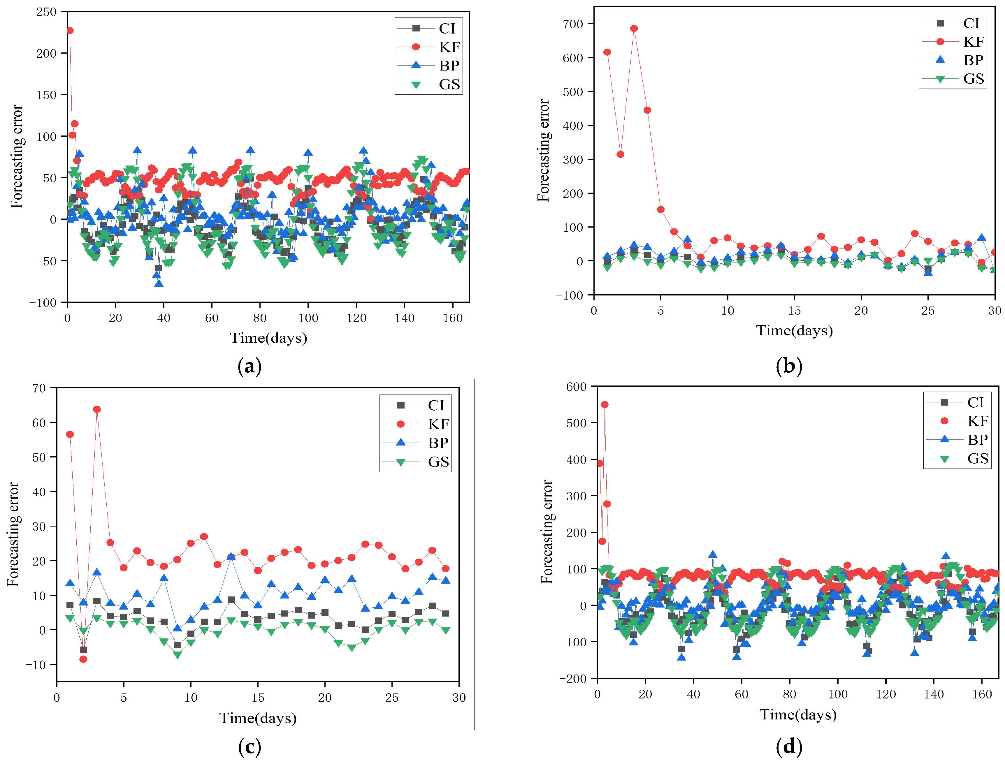
After substituting these parameters into (23) and using the MATLAB tool, the forecasting results by the CI for the entire year from July 2020 to July 2021 are presented by fusing the results from the three methods. Taking the four stages of the first quarter in the second year as an example, the forecasting results are shown in Figure 4, where the forecasting results are evaluated by the error between each real load and the computed load.

The forecasting loads by the CI fusion method have reduced the problems of large errors in the first three sampling points of the KF, large errors in individual points of the BP method, and exponential changes in the forecasting values of the GS method. The forecasting errors of the proposed CI fusion for the four quarters are shown in

Table 7. Forecasting errors by CI in seven stages (Unit: MW).

Stage	Maximal Absolute Error	Average Maximal Error	Average Relative Error	Standard Error
1	30.121	26.456	3.2%	7.263
2	12.654	10.337	2.8%	3.188
3	109.221	83.704	11.8%	30.126
4	46.139	40.659	10.4%	20.783
5	70.853	50.760	12.8%	28.491
6	43.573	37.327	9.1%	30.328
7	44.205	36.663	9.7%	20.393

.

Compared with the respective forecasting results from the KF, BP, and GS, the fusion results by the CI from Table 7 can be summarized as follows.

(1) The maximum forecasting error among the three methods occurs in the KF method. Although KF is a continuous iterative process, the errors at the initial points and the increase in subsequent errors can cancel each other out, and the subsequent filtering tends to stabilize. However, due to the significant errors at the first three points, the maximum errors still have a significant impact on the overall accuracy of load forecasting, resulting in various error indicators being less favorable compared to other methods.

(2) For stages 1 and 2, the GS forecasting results show the minimum average relative error, because this stage corresponds to the minimum fluctuation of the load value at the morning time of each day, and the GS model is well-suited for load forecasting with relatively flat data changes. The forecasting results of the CI fusion method are affected by the large forecasting error of the KF method, leading to inferior results compared to the GS in some stages. However, it weakens the instability and limitations of single forecasting results of both KF and the BP neural network.

(3) Comparing the errors of three single forecasting methods, the average relative error from the CI fusion forecasting results is the smallest, which overall reduces the instability and limitations of the single forecasting results of the other three methods in various stages. The advantages of the CI fusion method are obvious.

4. Conclusions

This study aims to address the issues of imprecision, uncertainty, and instability in short-term power load forecasting using a single method. A new fusion method using the Choquet integral is proposed. This method can fully use the interactions and complementarity among various methods, leading to the more accurate and stable forecasting results of short-term loads. Different from the other existing methods, the proposed fusion method can effectively exact the key features and parameters in the fusion process by using a typical optimization algorithm, which is very easily realized and understood in practice. Therefore, the proposed method provides new ideas and a practical means for fusing multimodal and multi-resource methods in short-term load forecasting, and it can be extended to any power system.

However, there is still room for improvement in the method proposed in this study. Firstly, further research and analysis are required on the typicality of the fused forecasting methods. Secondly, in the case of big data, current deep learning-based methods can be used to further evaluate and compare the advantages, disadvantages, and usability of the proposed method. Finally, an applicable method must be chosen to conduct a more in-depth analysis of the various factors that affect the operation of the power system and load changes, in order to effectively improve the accuracy of short-term load forecasting.