Article

Identification of Sub-Synchronous Oscillation Mode Based on HO-VMD and SVD-Regularized TLS-Prony Methods

by
Yuzhe Chen
,
Feng Wu
*,
Linjun Shi
,
Yang Li
,
Peng Qi
and
Xu Guo
College of Energy and Electrical Engineering, Hohai University, Nanjing 211100, China
*
Author to whom correspondence should be addressed.
Energies 2024, 17(20), 5067; https://doi.org/10.3390/en17205067
Submission received: 26 August 2024 / Revised: 6 October 2024 / Accepted: 10 October 2024 / Published: 11 October 2024

Abstract

:
To reduce errors in sub-synchronous oscillation (SSO) modal identification and improve the accuracy and noise resistance of the traditional Prony algorithm, this paper focuses on SSOs caused by the integration of doubly fed induction generators (DFIGs) with series compensation into the grid. A novel SSO modal identification method based on the hippopotamus optimization–variational mode decomposition (HO-VMD) and singular value decomposition–regularized total least squares–Prony (SVD-RTLS-Prony) algorithms is proposed. First, the energy ratio function is used for real-time monitoring of the system to identify oscillation signals. Then, to address the limitations of the VMD algorithm, the HO algorithm’s excellent optimization capabilities were utilized to improve the VMD algorithm, leading to preliminary denoising. Finally, the SVD-RTLS-improved Prony algorithm was employed to further suppress noise interference and extract oscillation characteristics, allowing for the accurate identification of SSO modes. The performance of the proposed method was evaluated using theoretical and practical models on the Matlab and PSCAD simulation platforms. The results indicate that the algorithms effectively perform denoising and accurately identify the characteristics of SSO signals, confirming its effectiveness, accuracy, superiority, and robustness against interference.

1. Introduction

To mitigate the energy shortages and environmental degradation, countries worldwide are actively advancing energy transitions [1,2]. The share of traditional coal-fired power in the energy mix is gradually decreasing, while the proportion of new clean energy sources, such as wind power, is steadily increasing. However, the intermittent, volatile, and unpredictable nature of these renewable energy sources presents new challenges for the stable operation of power grids [3,4,5,6,7]. Among these challenges, sub-synchronous oscillations (SSOs) induced by wind power plants (WPPs) integrated into the grid through series compensation are one of the most representative phenomena and pose a significant threat to the stability and security of power systems [8,9,10]. For instance, in 2009, a wind farm in Texas, USA, experienced SSOs induced by the integration of renewable energy sources [11,12]. Similar SSO incidents have also been reported in the Buffalo Ridge zone of Canada [13] and in parts of northwest China [14,15]. Consequently, promptly identifying oscillation modes through real-time status monitoring and using modal identification algorithms to detect oscillation factors before they cause significant damage to the system is crucial for ensuring the safe and stable operation of power systems [16].
Modern power system identification and detection methods can be broadly categorized into time-domain, frequency-domain, and time–frequency-domain approaches [17]. Among these, time-domain methods are the most commonly used. Examples include the traditional Prony algorithm [18], the rotation invariant technology used to estimate signal parameters [19,20], Dynamic Mode Decomposition (DMD) [21], and the matrix pencil method [22]. However, these methods require a certain level of understanding of the model, and preset parameters can significantly influence the results. Additionally, these methods are highly sensitive to signal quality; if the signal is noisy, the identification results can be adversely affected. To address this issue, signal modal decomposition and reconstruction can be employed to effectively filter out noise, thereby improving identification accuracy.
Common signal decomposition methods include Empirical Mode Decomposition (EMD) [23], Ensemble Empirical Mode Decomposition (EEMD) [24], Wavelet Transform (WT) [25], Empirical Wavelet Transform (EWT) [26], and Local Mean Decomposition (LMD) [27]. These algorithms have been widely used in various fields, but they also face challenges affecting the effectiveness of signal decomposition. EMD often encounters mode mixing and endpoint effects during signal decomposition. EEMD improves the mode mixing issue of EMD to some extent, but determining the amplitude of the added white noise is challenging [28]. WT lacks flexibility due to the fixed choice of mother wavelet, resulting in poor adaptability when processing different types of signals. EWT overly relies on the accurate segmentation of the spectrum [29]. The LMD method may also be affected by modal aliasing caused by intermittent components in the signal during the signal decomposition process [30]. Dragomiretskiy et al. [31] proposed the variational mode decomposition (VMD) method. Compared to methods like WT and EMD, VMD offers advantages in signal decomposition with higher accuracy, faster convergence, and better robustness. However, the effectiveness of the VMD algorithm can be limited by the number of Intrinsic Mode Functions (IMFs), denoted as the number of decomposition modes K, and the penalty factor parameter α. Improper parameter settings may lead to mode mixing issues. To overcome these limitations, many researchers have employed various optimization methods for adaptive parameter adjustments. For instance, Li et al. [32] used a genetic algorithm to adaptively search for the optimal VMD parameters, Liu et al. [33] applied the Grey Wolf Optimizer to obtain the best parameters for VMD. Du et al. [34] utilized the Sparrow Search Algorithm based on the Halton sequence and Laplace crossover operator (HLSSA-VMD) to optimize VMD parameters. Meng et al. proposed an optimized VMD method based on modified scale-space representation (MSSR-VMD), which can adaptively obtain the number of modes and the initial center frequency for each mode [35]. Guo et al. proposed an improved gravitational search algorithm (IGSA) with a nonlinear decreasing inertia weight factor, which is integrated into the VMD for the adaptive selection of two parameters [36]. The application of these optimization algorithms has significantly improved the effectiveness and accuracy of VMD in signal processing. However, issues remain due to the overlap and lack of diversity in initial solutions, which can cause the algorithm to become trapped in local optima and result in slow convergence speed.
Based on the aforementioned research and shortcomings, this paper proposes an hippopotamus optimization–VMD (HO-VMD) method that utilizes the energy ratio function for detection and incorporates the HO algorithm proposed by Amiri et al. [37] for the fuzzy entropy optimization iteration of the IMFs derived from VMD. Additionally, the singular value decomposition–regularized total least squares–Prony (SVD-RTLS-Prony) algorithm is employed for modal identification. Validation through both theoretical and practical models demonstrates the effectiveness and accuracy of this method, providing theoretical guidance and technical support for subsequent broadband oscillation analysis in power systems.

2. Fundamental Principles of the Identification Algorithm

2.1. Ideal Mathematical Model of SSO

The SSO signal can be represented as a sum of exponentially decaying or diverging sinusoidal waves, expressed in the following form [38]:
x ( t ) = i = 1 n A i e ξ i t sin 2 π f i t + φ i
where A i , ξ i , f i , and φ i represent the relative amplitude, damping factor, frequency, and phase shift of the i -th oscillatory component in x ( t ) , respectively. The ultimate goal of modal identification is to accurately determine each parameter of these oscillatory components, thereby gaining a better understanding of the system’s operational state.

2.2. Principles and Shortcomings of the VMD Algorithm

When using the Prony algorithm to identify oscillatory modes in power systems, it is highly sensitive to noise and requires high-quality sampled signals, making it necessary to first apply denoising and filtering processes. Compared to the traditional EMD, the VMD algorithm is supported by a more rigorous mathematical theory, which helps to better avoid mode mixing and offers improved noise resistance. Therefore, to enhance the accuracy of the Prony algorithm in identifying oscillation signal modes, the sampled signals are first preprocessed with VMD-based filtering and denoising. The specific process of VMD preprocessing is as follows [39]:
Stage 1: Set the number of decomposition modes K, the penalty factor α, and initialize the mode functions u k and center frequencies ω k . The expression for the mode components is as follows:
u k ( t ) = A k ( t ) cos φ k ( t )
where t represents the time series, and A k ( t ) and φ k ( t ) denote the instantaneous amplitude and instantaneous phase, respectively.
Stage 2: Hilbert Transform (HT) is used to compute the single-sided spectrum of each u k ( t ) , which is then multiplied by an indicator function e j ω k t raised to the power of the center frequency ω k , shifting each component to the baseband. The L 2 norm is used to estimate the bandwidth of each mode component, with the corresponding constrained variational model expressed as follows:
min u k , ω k k t δ ( t ) + j π t u k ( t ) e j ω k t 2 2   s .   t . k u k ( t ) = f ( t )
Stage 3: Introduce the quadratic penalty factor α and the Lagrange multiplier λ to solve the variational problem, transforming the constrained problem into an unconstrained one. The resulting Lagrange expression is as follows:
L u k , ω k , λ = α k t δ ( t ) + j π t u k ( t ) e j ω k t 2 2 + f ( t ) k u k ( t ) 2 2 + λ ( t ) , f ( t ) k u k ( t )
Stage 4: The Alternating Direction Method of Multipliers (ADMM) is used to iteratively update the spectral components and the center frequencies of each mode. The update expressions for the spectral components u ^ k and the center frequencies ω k are as follows:
u ^ k n + 1 ( ω ) = f ^ ( ω ) i k u ^ i ( ω ) + λ ^ ( ω ) / 2 1 + 2 α ω ω k 2
ω k n + 1 = 0 ω u ^ k ( ω ) 2 d ω 0 u ^ k ( ω ) 2 d ω
where u ^ k n + 1 , f ^ ( ω ) , λ ^ ( ω ) represent the Fourier transforms of u k n + 1 , f ( ω ) , and λ ( ω ) , respectively.
As indicated by Equation (2), the number of decomposition modes K affects the estimation of instantaneous frequency, and an inappropriate choice of K can lead to mode mixing. If K is set too high, it will result in over-decomposition; conversely, if K is too low, it will lead to under-decomposition. According to Equations (5) and (6), the penalty factor α influences the bandwidth of the IMFs; setting α too high will cause a loss of frequency band information, while setting it too low will lead to information redundancy. Therefore, selecting appropriate parameters is crucial for the accurate VMD of signals. However, in practical applications, the actual number of modes in the sampled signal is often unknown. Manually setting parameters introduces a high degree of subjectivity, making it difficult to ensure the accuracy of the decomposition. Consequently, it is necessary to introduce an optimization algorithm that can adaptively adjust and determine the most suitable parameter values for the sampled signal.

2.3. VMD Algorithm Improved Based on HO Algorithm

To address the issue that traditional VMD algorithms are significantly affected by the initial parameters, this paper proposes an improved VMD algorithm based on the HO algorithm. It uses the HO algorithm to find the optimal input coefficients. The HO algorithm, conceived by Mohammad Hussein Amiri and colleagues, draws inspiration from the inherent behaviors observed in hippopotamuses. This algorithm aims to solve complex optimization problems by balancing exploration and exploitation, thereby efficiently searching for the optimal solution. Compared to methods like WOA, GWO, SSA, and PSO, the hippopotamus optimization algorithm demonstrates high efficiency and strong adaptability [37]. HO is a population-based optimization algorithm, where the search agents are represented by hippopotamuses. In the HO-VMD algorithm, the position of each hippopotamus in the search space represents the values of the decision variables. Similar to traditional optimization algorithms, the initialization phase of HO involves the generation of random initial solutions. The iterative process of HO can be divided into three stages.
Stage 1: Position update of hippopotamuses in rivers or ponds. In this stage, the dominant hippopotamus (the best solution in the population) is identified, and the position update models for male, female, and juvenile hippopotamuses are established based on this dominant individual.
Stage 2: Hippopotamus defense against predators. When a hippopotamus is attacked by a predator, it turns towards the predator and emits loud vocalizations to scare it away. During this stage, the hippopotamus may exhibit behaviors that approach the predator, inducing it to retreat, effectively defending against potential threats.
Stage 3: Hippopotamus evasion of predators. If the hippopotamus cannot fend off the predator through defensive behavior, it will flee to the nearest water body. This behavior is simulated during the exploitation phase of local search.
After each iteration of the HO algorithm, all population members are updated according to the processes in stages 1 to 3, based on the respective formulas. This process continues until the final iteration. Throughout the execution of the HO algorithm, the best potential solution is continuously tracked and stored. Upon completion of the algorithm, the best candidate solution, referred to as the “dominant hippopotamus solution”, is revealed as the final solution to the problem.
Setting the decomposition mode K and penalty factor α as the hippopotamus position variables, the fuzzy entropy of the IMFs obtained from the VMD is used as the criterion for optimal position assessment. Fuzzy entropy is a metric used to measure the complexity and uncertainty of time series data. It is an entropy measurement method based on fuzzy set theory, designed to handle signal data with uncertainty and fuzziness. The larger the fuzzy entropy of a signal, the higher its complexity and uncertainty, and the greater the amount of noise it contains. Therefore, to ensure noise reduction performance while minimizing the number of decomposition modes and improving computational efficiency, the fitness function for the HO-VMD algorithm is defined as follows:
f i t n e s s = m i n ( F E ) + m e a n ( F E ) + 0.2 × s u m ( F E )
where FE(1, 2, …, K) represent the fuzzy entropy values of the K IMFs obtained from the VMD. The detailed process of the HO-VMD algorithm is illustrated in the flowchart shown in Figure 1. X i M h i p p o , X i F B h i p p o and X i represent male hippopotamus position and female or immature hippopotamus position and the position of i t h hippopotamus, respectively.

2.4. Improved Prony Identification Algorithm

The Prony algorithm can extract key characteristics of oscillatory signals, such as modal frequency, damping ratio, phase, and amplitude. However, it is highly sensitive to noise in actual power grid signals, making it susceptible to interference from data noise, which can result in false oscillation modes and reduced identification accuracy. Additionally, as the amount of data increases, the computational complexity escalates rapidly, potentially leading to issues like the curse of dimensionality in the Prony algorithm. To address these challenges, this paper integrates SVD with the regularized total least squares (RTLS) method to enhance the traditional Prony method. SVD is used to decompose the data matrix, while TLS handles measurement errors, thereby improving the accuracy of frequency and damping factor estimation and significantly enhancing noise robustness. The specific workflow of the SVD-RTLS-Prony algorithm is as follows [40,41]:
Stage 1: Hankel Matrix and SVD. The signal X = x 1 x 2 x 3 x N is structured into an m × n Hankel matrix.
H = x 1 x 2 x n x 2 x 3 x n + 1 x m x m + 1 x N
where N = m + n 1 . The anti-diagonal elements of the Hankel matrix are identical. The SVD of the Hankel matrix yields the following:
H = U m × m S m × n V H n × n
where U and V are the orthogonal matrices of dimensions m × m and n × n, respectively; S is an m × n singular value matrix, S = d i a g σ 1 , σ 2 , , σ r , 0   σ i represents the singular values, which are non-zero and arranged in descending order, and r is the rank of matrix S. The number of effective singular values k is selected, and the remaining singular values are set to zero, resulting in matrix S′. If k is too small, excessive noise reduction may occur, filtering out some useful signals; if k is too large, insufficient noise reduction may result, leaving some noise unfiltered, which could interfere with the identification results. In this scenario, the optimal number of decomposition modes K obtained from the iterative optimization results of the HO-VMD algorithm is introduced and proportionally scaled up to determine the appropriate number of effective singular values.
Stage 2: RTLS correction. Construct a new matrix R T L S and incorporate a regularization term as follows:
R T L S = H H H + λ I
where λ is the regularization parameter, and I is the identity matrix. Compared to conventional TLS, the introduction of RTLS provides additional stability to the matrix, enhancing the algorithm’s numerical stability when dealing with large-scale or high-dimensional data. RTLS offers significant advantages in noise suppression, handling ill-posed problems, model selection, generalization ability, and numerical stability.
Stage 3: Solving the characteristic polynomial. Perform eigenvalue decomposition on the regularized matrix R T L S to determine the effective rank p and the coefficients a 1 , a 2 , , a p corresponding to the oscillation modes. From this, the characteristic polynomial can be constructed, and its roots z , also known as Prony poles, can be solved. The characteristic polynomial is expressed as follows:
1 + a 1 z 1 + + a p z p = 0
Recursively obtain x ^ ( n ) based on x ^ k ( n ) = i = 1 p a i x ^ k ( n m ) , where x ^ k ( 0 ) = x k ( 0 ) . Based on this, the contribution of each mode in the signals can be calculated as follows:
1 1 1 z 1 z 2 z p z 1 N k 1 z 2 N k 1 z p N k 1 b k 1 b k 2 b k p = x ^ k ( 0 ) x ^ k ( 1 ) x ^ k N k 1
where N k represents the number of sampling points for the k-th signal. This can be simplified to Z b = x ^ k , yielding the following:
b k = Z H Z 1 Z H x ^ k
From this, the relevant components of each oscillatory mode can be calculated, including amplitude A k i , phase θ k i , frequency f i , and damping factor α i , where k represents the k-th signal and iii represents the i-th component. At this point, all dominant oscillation modes and their associated parameters in the output signal can be determined. Subsequently, the primary oscillatory modes are selected and output based on the optimal number of decomposition modes K.
A k i = b k i θ k i = arctan I m b k i Re b k i f i = arctan I m z i Re z i / 2 π Δ t α i = L n z i Δ t

2.5. Energy Ratio Function

For the identification of SSO, signal singularity detection is crucial to initiating the parameter identification process. Considering the practical detection performance and algorithm complexity, this paper employs the energy ratio function to initiate the detection of SSO. The Energy Ratio method determines signal anomalies by calculating the ratio of the effective values of energy in two segments within a fixed time window. This time window represents a fixed time interval that can be converted into a number of sampling points based on the sampling frequency. The calculation formula for the energy ratio E r is expressed as follows [38]:
E r = t = T 0 + T / 2 T 0 + T x 2 ( t ) 1 / 2 / t = T 0 T 0 + T / 2 x 2 ( t ) 1 / 2
where T represents the total length of the time window, E r is the energy ratio between the latter half and the former half of the time window, and T 0 is the starting point of the time window. When using the Energy Ratio method for singularity detection, it is essential to consider various factors to determine the appropriate window width, ensuring the accurate identification of oscillation occurrences. Additionally, a reasonable energy ratio threshold must be set to enable timely actions, such as shutting down equipment or disconnecting from the grid, once oscillations are detected, thereby preventing more severe incidents.

3. Specific Stages of the HO-VMD and SVD-RTLS-Prony Algorithms

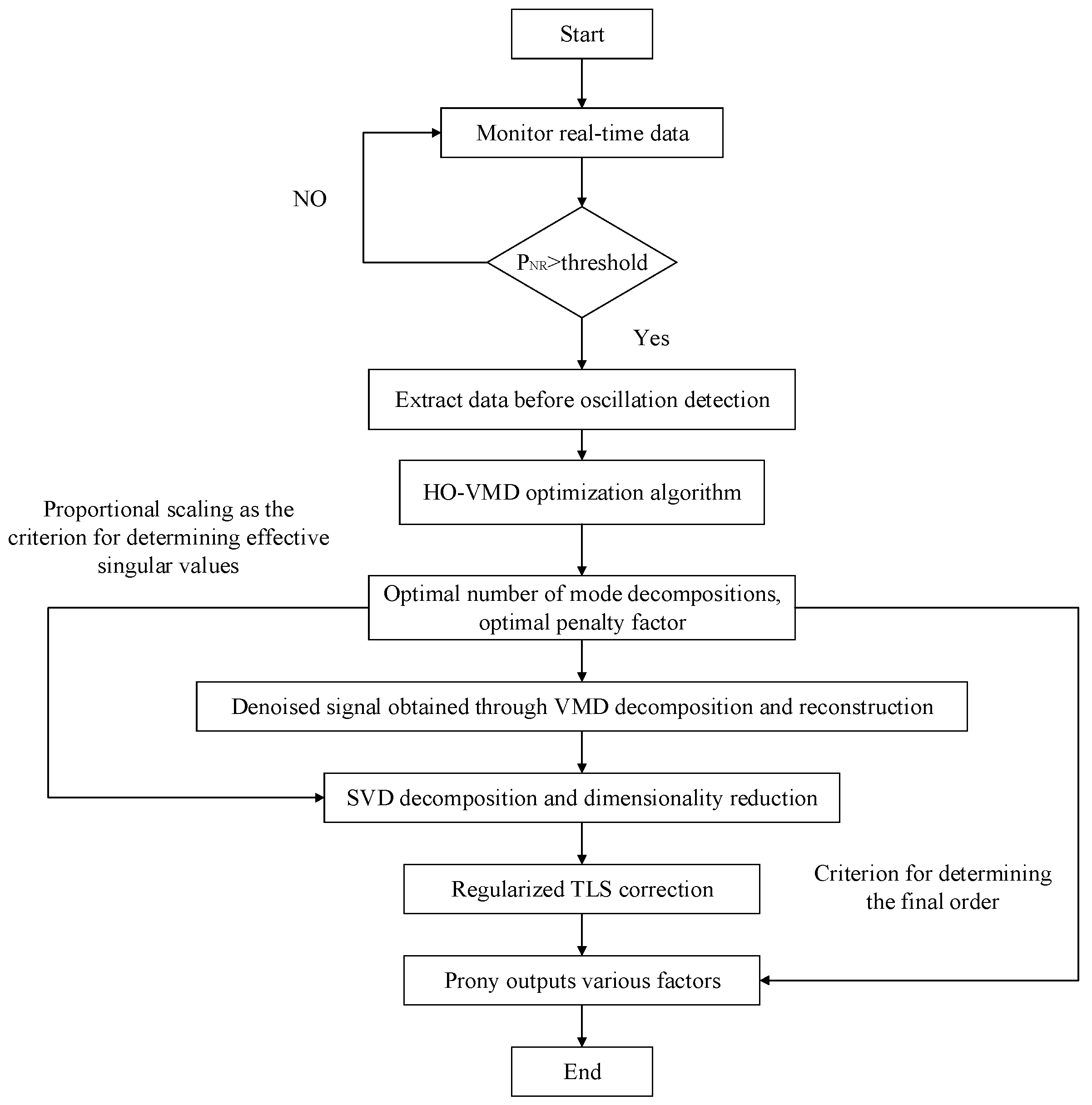
The real-time monitoring and modal identification algorithm for SSO based on HO-VMD and SVD-RTLS-Prony consists of five stages: E r real-time monitoring, HO-VMD denoising, SVD and dimensionality reduction, RTLS correction, and Prony output. The detailed flowchart is shown in Figure 2.
Stage 1: Real-Time Signal Energy Ratio Detection.
Begin real-time monitoring when the system is in a stable state. When oscillations occur, the source signal of the oscillation undergoes significant changes, leading to corresponding changes in the measured signal’s energy. The energy ratio E r is used to detect signal singularity, with the judgment criterion being E r ε . Here, ε is the preset threshold, which is related to the time window width and the system’s sampling frequency. If E r exceeds the preset threshold, the system initiates machine shutdown, and the real-time data collected just before the shutdown are used for subsequent analysis.
Stage 2: Preliminary Denoising Using the HO-VMD Algorithm.
Input the real-time data into the HO-VMD algorithm. The fuzzy entropy of the IMFs is used as the evaluation criterion to iteratively determine the optimal number of mode decompositions and the penalty factor. These parameters are then applied to the VMD algorithm to decompose the real-time data and reconstruct it, yielding denoised data.
Stage 3: SVD on Denoised Data.
Construct a data matrix for dimensionality reduction using SVD. The optimal number of mode decompositions obtained from the HO-VMD algorithm is proportionally scaled and used as a threshold to filter effective singular values.
Stage 4: Regularized TLS Correction.
Optimize the data matrix using regularized TLS to enhance model stability, reduce overfitting, address underdetermined problems, and suppress high-frequency noise. Perform eigenvalue decomposition on the data matrix, construct the characteristic polynomial, and determine the Prony nodes.
Stage 5: Prony Computation.
Using the characteristic polynomial and Prony nodes, perform computations to obtain parameters such as the amplitude, frequency, damping ratio, and phase of each oscillation mode.

4. Case Study

4.1. Ideal Signal Case Study

To validate the effectiveness of the HO-VMD and SVD-RTLS-Prony signal identification method proposed in this paper, an ideal SSO signal is constructed, and the oscillation modes of the signal are extracted for simulation analysis. To demonstrate the applicability of this method, the constructed ideal sub-synchronous signal is designed with significantly different modes. The ideal signal is constructed as follows:
x ( n ) = 272 e 0.42 t cos ( 2 π × 15.6 t + π / 8 ) + 258 e 0.16 t cos ( 2 π × 32.4 t + π / 4 ) + 160 e 0.28 t cos ( 2 π × 47.6 t )
Since actual SSO signals often contain Gaussian noise, Gaussian white noise is added to the ideal signal in this study to test the algorithm. The 12 dB Gaussian white noise sequence used in this study is generated by Matlab (version number R2020b), with a mean of 0 and a variance of 1. The signal simulation duration is 3 s, with a time step of 0.001 s. The resulting ideal signal and noisy signal are shown in Figure 3.
To validate the superiority of the HO-VMD algorithm used in this paper for noise reduction, the traditional EMD and VMD algorithms are used as comparisons. The signal-to-noise ratio (SNR) and mean square error (MSE) between the reconstructed signal and the ideal signal after decomposition are calculated as evaluation metrics for the quality of the denoised signal. The better the denoising effect of the algorithm, the higher the SNR value and the lower the MSE value between the ideal signal and the reconstructed signal. The calculation formulas are as follows:
S N R = 10 lg i = 1 N x 1 2 ( i ) i = 1 N x 1 ( i ) x 2 ( i ) 2
M SE = i = 1 N x 1 ( i ) x 2 ( i ) 2 N
where x 1 and x 2 represent the ideal signal and the reconstructed signal, respectively. The number of mode decompositions K is set to 3, 5, and 7, with the penalty factor α set to 500, 1000, and 2000. The EMD and VMD algorithms are applied to decompose and reconstruct the noisy signal, and the results are shown in Table 1.
As shown in Table 1, the denoising performance of the VMD algorithm is superior to that of the EMD algorithm when the number of decomposition modes is the same. Additionally, different K and α significantly affect the decomposition results, making it evident that manually setting these parameters is not ideal.
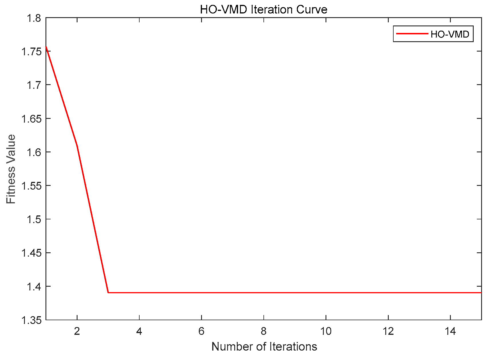
This confirms the necessity of using the HO algorithm. The results of modal decomposition and reconstruction of the noisy signal using the HO-VMD algorithm are shown in Figure 4.
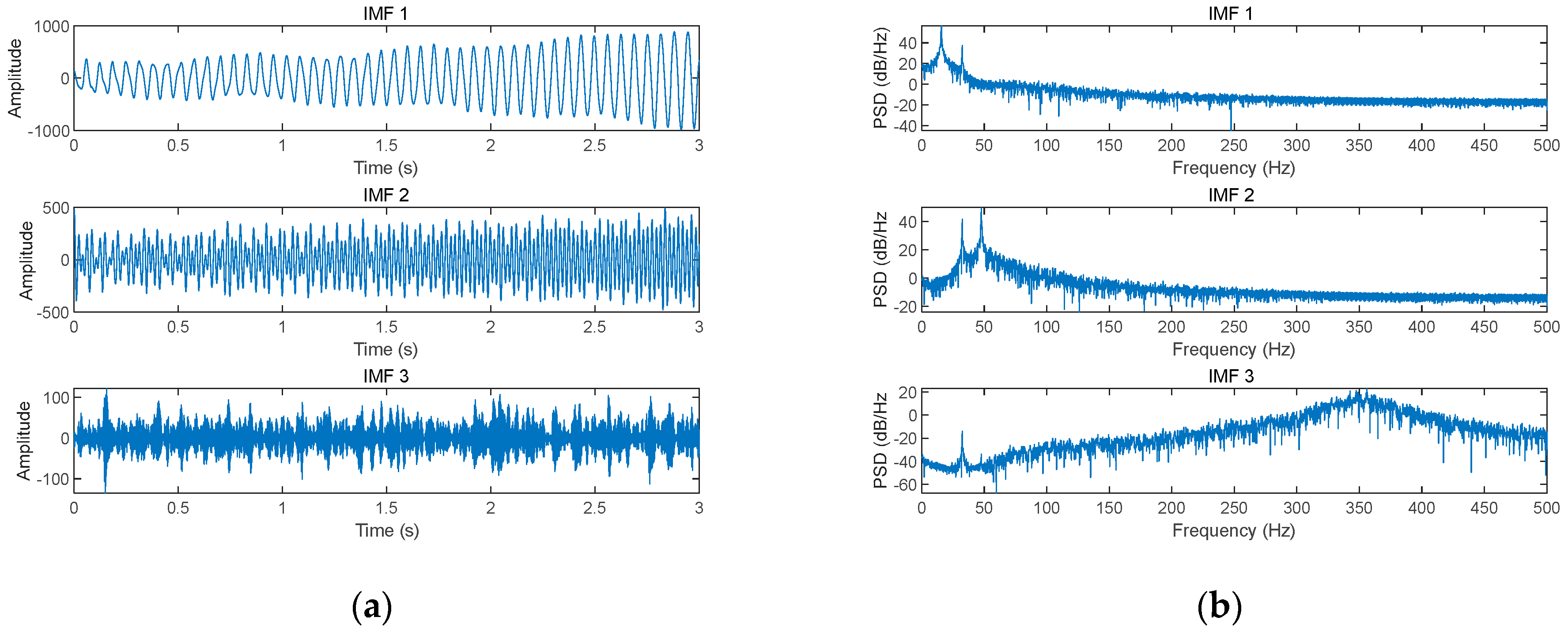
According to the optimization results of the HO-VMD algorithm, the optimal number of mode decompositions K is 3, and the optimal penalty factor α is 1638. Using these parameters, the noisy signal was decomposed using VMD, and the results are shown in Figure 5.
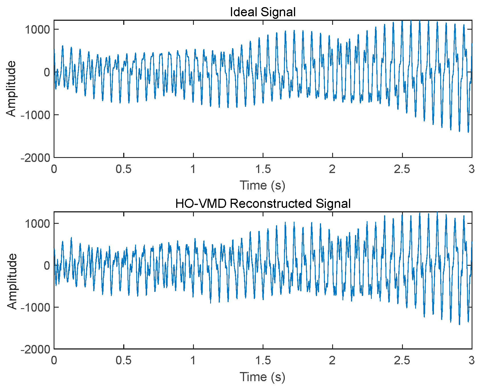
The IMFs were reconstructed and compared with the ideal signal, and the results are in Figure 6.
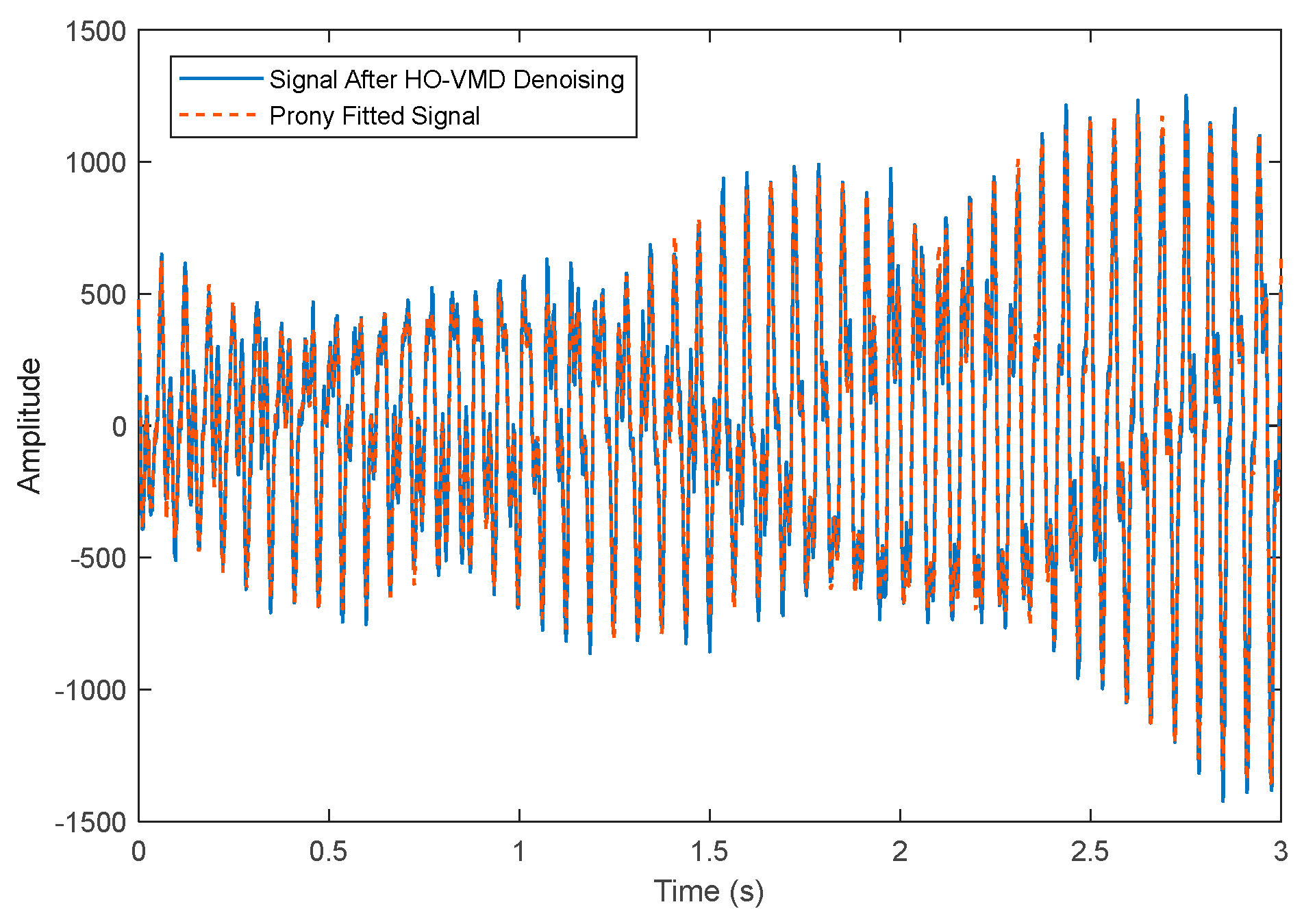
The calculation shows that the SNR between the HO-VMD-reconstructed signal and the ideal signal is 18.14 dB, and the MSE is 3396.17. Both are significantly better than those of the EMD and traditional VMD algorithms in Table 1, demonstrating that the HO-VMD algorithm proposed in this paper efficiently finds the optimal parameters and offers superior noise reduction performance, closely approximating the ideal signal. By inputting the HO-VMD-reconstructed signal into the SVD-TLS-Prony algorithm, the identification results are obtained as shown in Table 2. The signal refitted based on the identification results and the HO-VMD reconstructed signal are shown in Figure 7 and Table 2.
In Equation (16), the amplitudes, frequency, and damping factor of the three oscillatory components we set are as follows: 272, 15.6, and 0.42 for signal component 1; signal 258, 32.4, and −0.16 for signal component 2; and 160, 47.6, and 0.28 for signal component 3. By comparing them with the values in Table 2, it is evident that the method proposed in this paper accurately identifies the characteristics of signal component 1 and signal component 3. While the frequency and damping factor of oscillation signal component 2 are identified with reasonable accuracy, there is a certain deviation in its amplitude. This is because signal component 2 is a rapidly decaying signal that disappears quickly, making it more challenging to identify. This indicates that the SVD-RTLS-Prony algorithm used in this paper has a certain level of noise resistance in modal identification, allowing for the accurate identification of various factors of the oscillatory modes. The ideal signal case study strongly demonstrates the effectiveness and accuracy of the HO-VMD and SVD-RTLS-Prony algorithms proposed in this paper for SSO mode identification.

4.2. Practical Signal Case Study

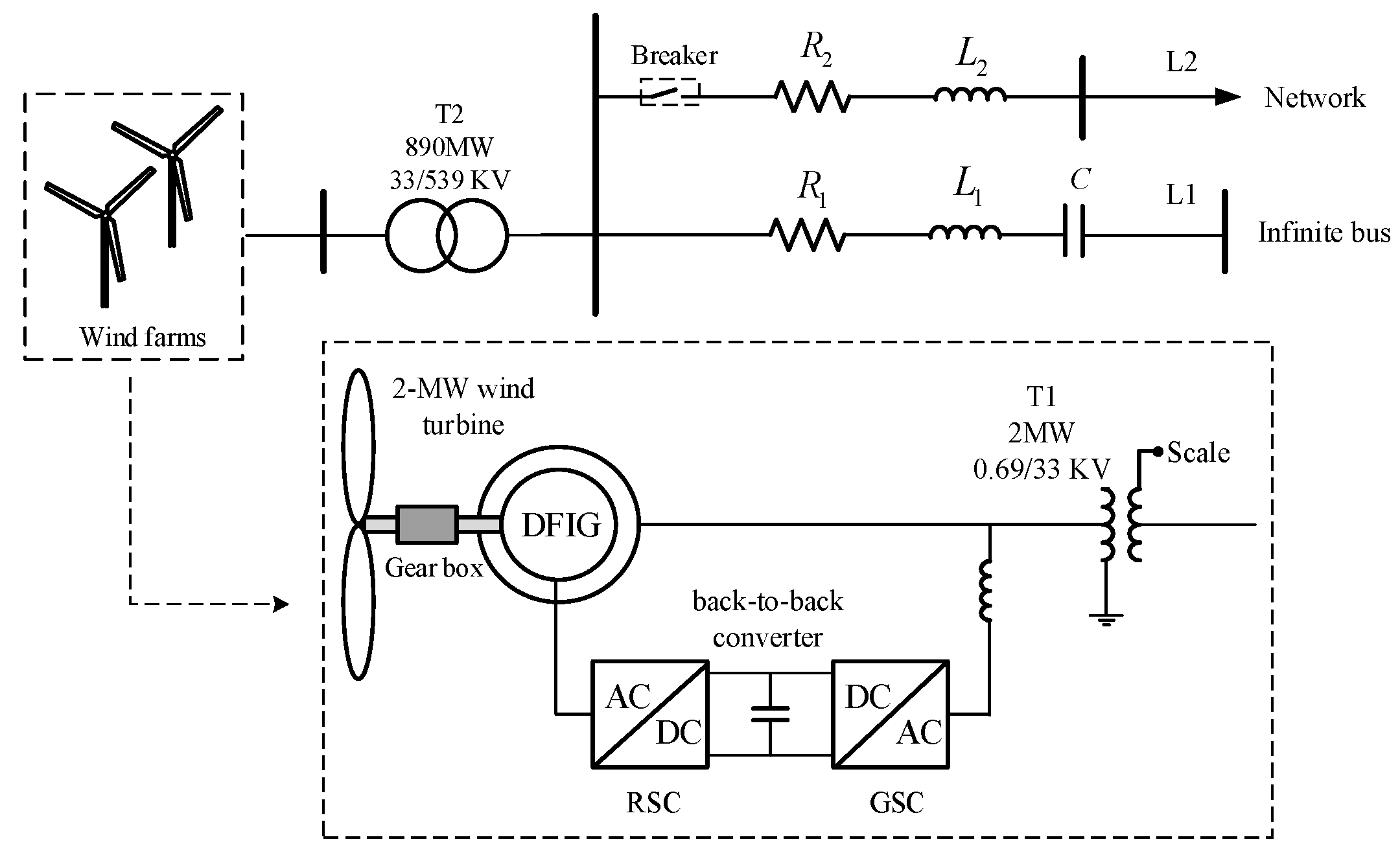
In this study, the modified IEEE First Benchmark Model is used as the research object to investigate SSO triggered by the integration of wind power systems into the grid through series-compensated lines. The structure is shown in Figure 8. In the figure, the DFIG is a standard 2 MW model connected to the grid through a 0.69/33 kV step-up transformer T1 [42]. By adjusting the scale factor of T1, the total capacity of the wind farm connected to the grid can be simulated. The scale factor set in this paper is 445. The DFIG wind farm is connected to the high-voltage transmission line through a 33/539 kV step-up transformer T2, with series compensation capacitors installed on transmission line L1. To simulate the occurrence of SSO in an actual power grid, transmission line L2 is disconnected at a specific moment, resulting in the radial connection of the DFIG wind farm to the series-compensated line [43]. This setup allows for the study of SSO under different line compensation levels. In the below figure, RSC represents the rotor-side converter, and GSC represents the grid-side converter of the DFIG. The main parameters of the wind power system are listed in Appendix A.
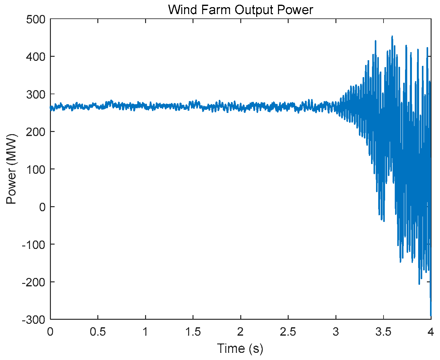
The above model is built in the PSCAD (version number 4.5) simulation software, with the line series compensation set to 40%. Line L2 is disconnected at the 3rd second after the system reaches stable operation. The system’s output power is shown in Figure 9.
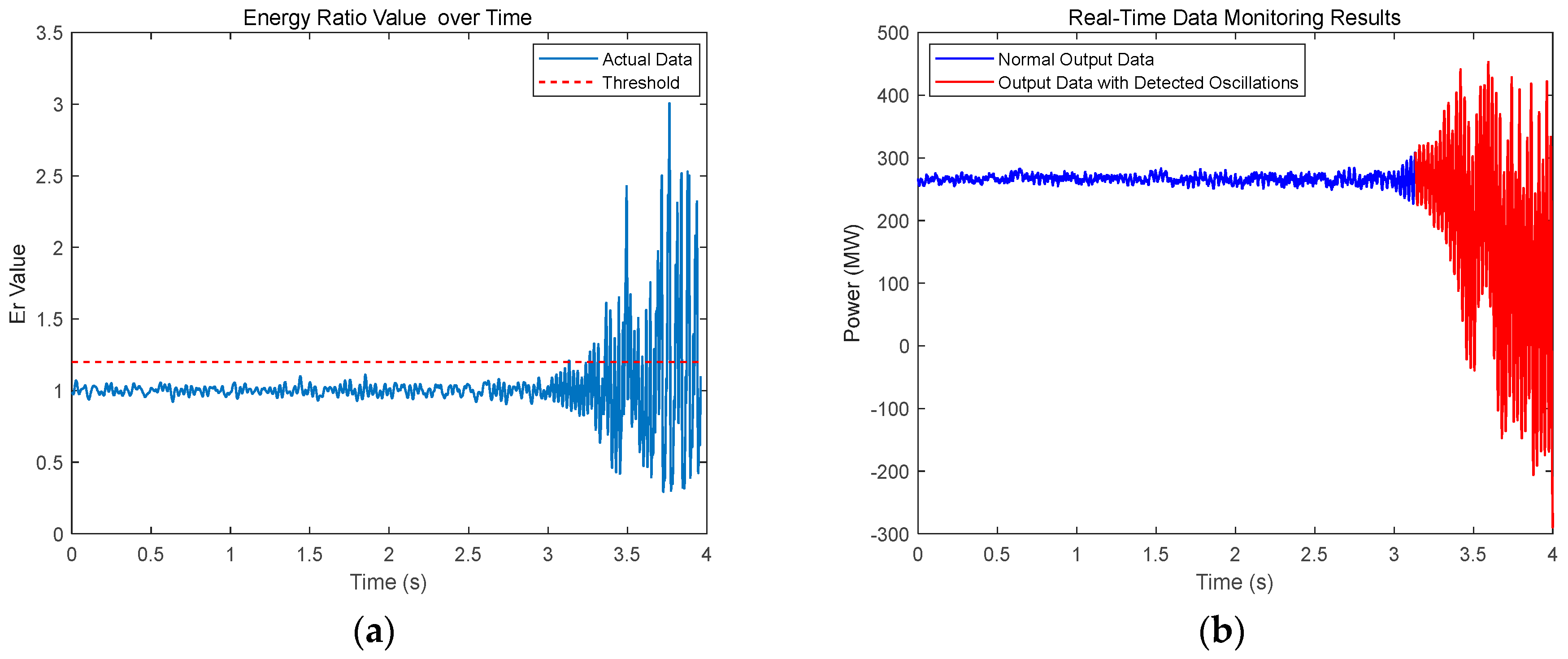
As shown in Figure 9, the system operates stably during the 0–3 s period, and oscillations occur at the 3rd second due to the disconnection of line L2. The real-time data of the system’s output power is monitored using the energy ratio function starting from the 0th second. If the energy ratio exceeds the set threshold, shutdown is initiated. The detection results are shown in Figure 10.
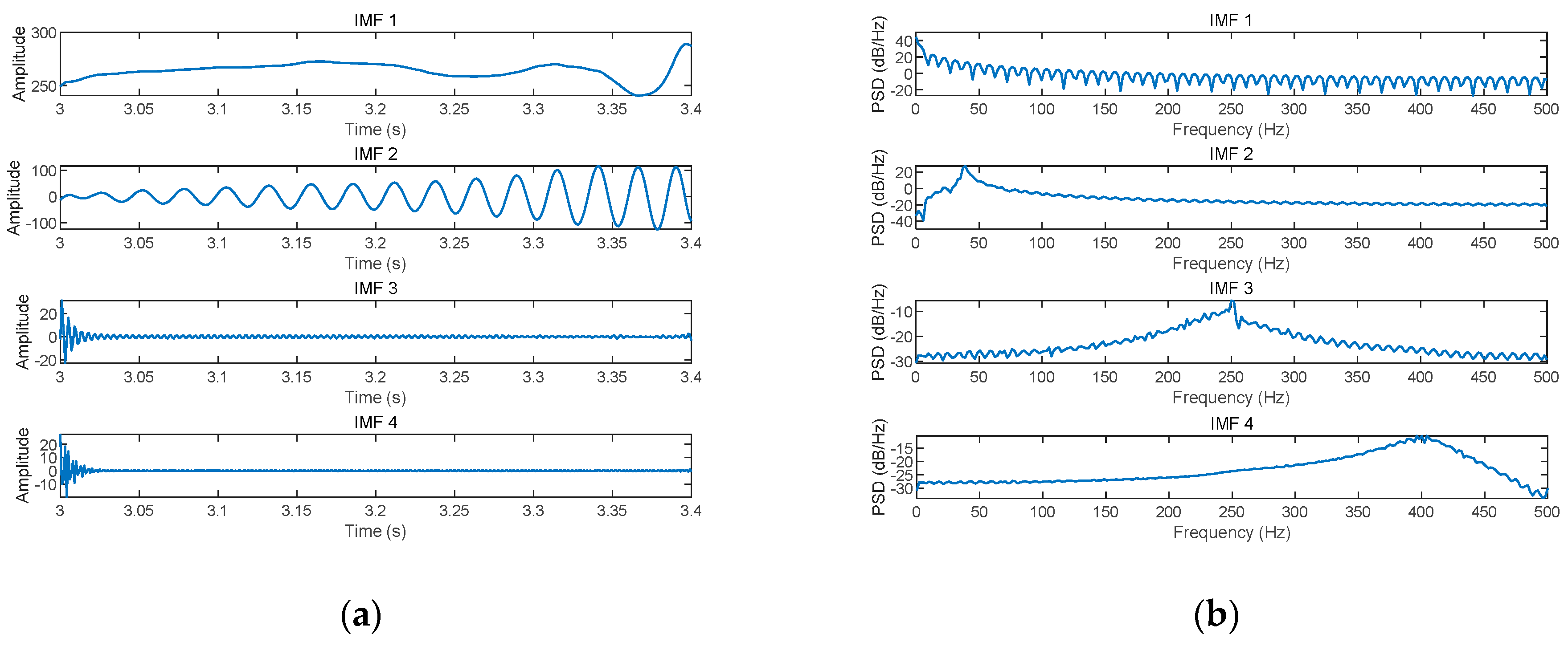
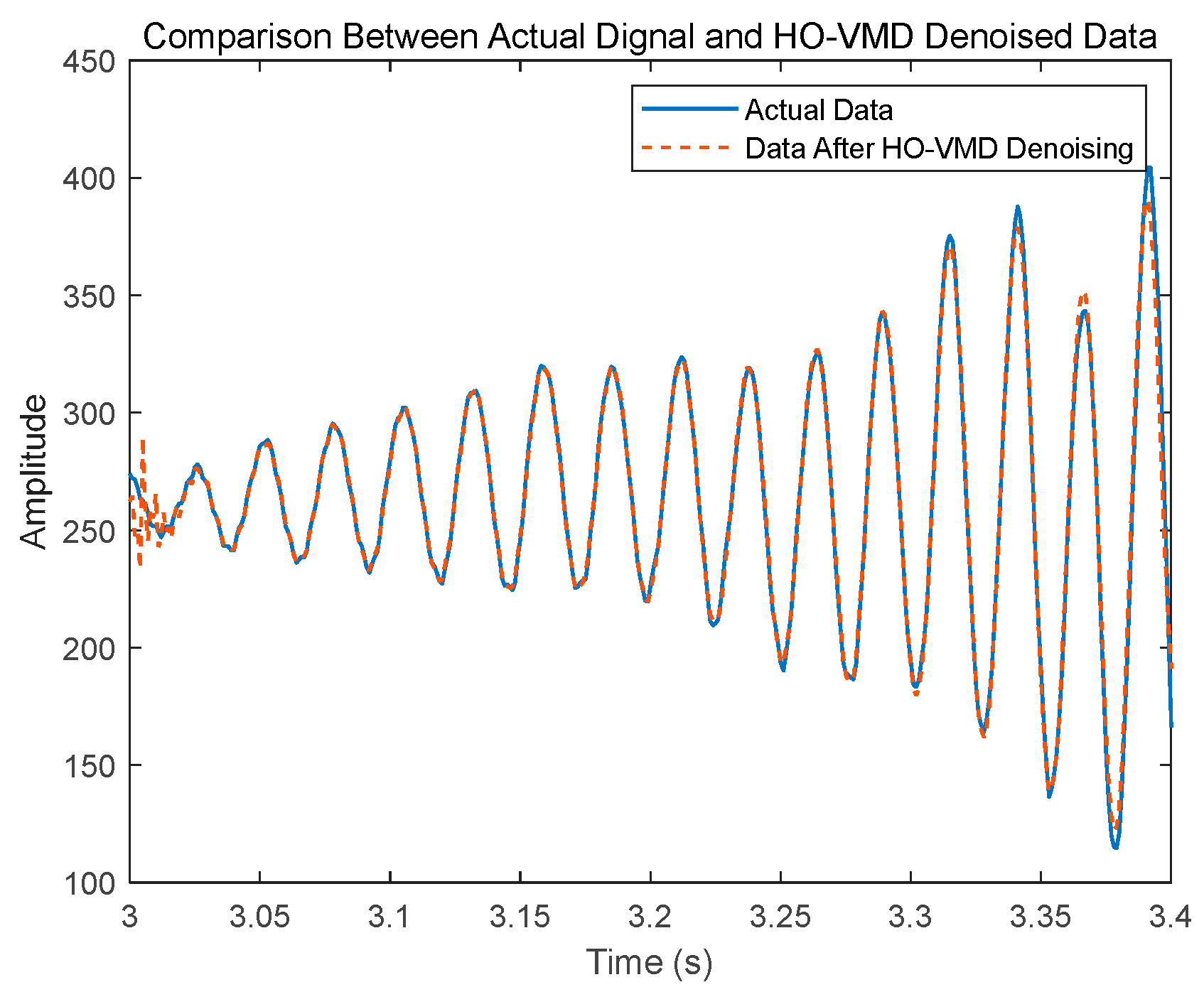
As shown in Figure 10, real-time monitoring detected that the energy ratio function exceeded the threshold at 3.174 s, triggering the shutdown process. In Figure 10, the blue section represents the system’s output power during normal operation, while the red section represents the oscillatory power that was prevented by the timely shutdown. This demonstrates that the real-time monitoring system quickly identified the system’s oscillations and initiated the shutdown, thereby avoiding a more severe incident. To further identify the details of the system’s oscillations, considering that the system requires approximately 0.2 s to react from detection to trip the unit, the data from 3 to 3.4 s were used for modal identification. The actual data were processed using the HO-VMD algorithm, with optimal parameters selected for decomposition and reconstruction. The preliminary denoising results are shown in Figure 11 and Figure 12.
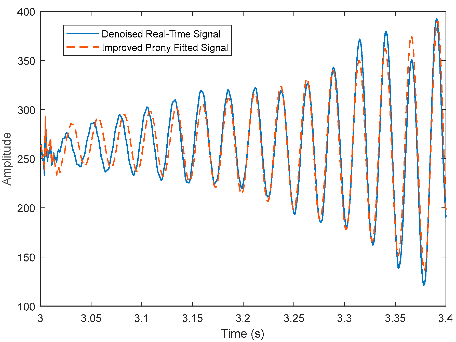
The HO-VMD algorithm identified the optimal number of mode decompositions K as 4 and the best penalty factor α as 1747. The denoised signal was then subjected to SVD-RTLS-Prony identification, with the identification results shown in Table 3. A comparison between the refitted signal based on these results and the denoised real-time signal is shown in Figure 13.
As shown in Table 3, the system’s main oscillatory mode is an SSO with a frequency of 39.82 Hz, exhibiting a divergent trend. To verify the validity of the identification results, a state-space model of the DFIG wind farm in the actual case was established, and its eigenvalues were calculated. With a line series compensation degree of 40%, the system has only one set of eigenvalues with a positive real part, which is 3.28 ± 261.24i, corresponding to a frequency of 41.58 Hz and a damping ratio of −1.26%. These results show a small error compared to the modal identification results, further validating the accuracy of the HO-VMD and SVD-RTLS-Prony method proposed in this paper.

5. Conclusions

This study proposes an SSO modal identification method based on the HO-VMD and SVD-RTLS-Prony algorithms. The energy ratio function is employed as a real-time detection indicator to determine the occurrence of SSOs. The HO-VMD algorithm is then used to find the optimal number of mode decompositions and penalty factors, thereby enhancing the precision of signal decomposition and performing noise reduction. Subsequently, the SVD-RTLS-Prony algorithm is applied to the denoised signal for accurate modal identification, extracting parameters such as the frequency and damping ratio of the oscillatory modes. The superiority of the HO-VMD algorithm is validated through the analysis of both ideal signal cases and practical signal cases. Compared to traditional EMD and VMD algorithms, the HO-VMD algorithm shows significant improvements in noise reduction. Additionally, this study demonstrates the effectiveness and accuracy of the proposed HO-VMD and SVD-RTLS-Prony algorithms in the identification of SSO modes and related factors triggered by power system grid integration. This provides theoretical support and technical reference for the diagnosis and treatment of SSO issues in power systems.

Author Contributions

Conceptualization, Y.C.; methodology, Y.C.; software, Y.C.; validation, Y.C.; formal analysis, X.G. and P.Q.; investigation, Y.C.; resources, L.S. and Y.L.; data curation, Y.C.; writing—original draft preparation, Y.C.; writing—review and editing, F.W. and L.S.; visualization, X.G. and P.Q.; supervision, L.S. and Y.L.; project administration, F.W.; funding acquisition, F.W. All authors have read and agreed to the published version of the manuscript.

Funding

This research was funded by NSFC, U23B20140.

Data Availability Statement

The original contributions presented in the study are included in the article, further inquiries can be directed to the corresponding author.

Conflicts of Interest

The authors declare no conflicts of interest.

Appendix A

Parameters of DFIG:
Rated Power:2 MW
Rated Voltage:0.69 kV
Frequency:60 Hz
Stator Resistance:0.00488 pu
Rotor Resistance:0.005491 pu
Stator Leakage Inductance:0.09231 pu
Rotor Leakage Inductance:0.09955 pu
Stator-Rotor Mutual Inductance:3.95279 pu
DC Side Capacitance:0.104 F
Parameters of Two-Mass Model:
Rotor Inertia Constant: 0.4 sWind Turbine Inertia Constant: 4 s
Stiffness Coefficient: 0.3 puDamping Coefficient: 0.01 pu
Parameters of Controller
K p 1 = 3 K i 1 = 1 / 0.3
K p 2 = 3 K i 2 = 1 / 0.1
K p 3 = 0.8 K i 3 = 1 / 0.1
K p 4 = 10 K i 4 = 1 / 0.01
K p 5 = 10 K i 5 = 1 / 0.01
Parameters of Lines in Figure 1
R 1 = 6.471   ohm R 2 = 0.001   ohm
L 1 = 0.1014   ( H ) L 1 = 0.1   ( H )
L T 1 = 0.1   pu L T 2 = 0.1   pu
C = 115.6   uF

References

  1. Cheng, Y.Z.; Fan, L.L.; Rose, J.; Huang, S.H.; Schmall, J.; Wang, X.Y.; Xie, X.R.; Shair, J.; Ramamurthy, J.R.; Modi, N.; et al. Real-World Subsynchronous Oscillation Events in Power Grids With High Penetrations of Inverter-Based Resources. IEEE Trans. Power Syst. 2023, 38, 316–330. [Google Scholar] [CrossRef]
  2. Liu, G.; Liu, J.; Liu, A.D. Mitigating sub-synchronous oscillation using intelligent damping control of DFIG based on improved TD3 algorithm with knowledge fusion. Sci. Rep. 2024, 14, 14692. [Google Scholar] [CrossRef] [PubMed]
  3. Schmidt, J.; Kemmetmüller, W.; Kugi, A. Modeling and static optimization of a variable speed pumped storage power plant. Renew. Energy 2017, 111, 38–51. [Google Scholar] [CrossRef]
  4. Ma, X.; Wu, D.; Wang, D.X.; Huang, B.W.; Desomber, K.; Fu, T.; Weimar, M. Optimizing pumped storage hydropower for multiple grid services. J. Energy Storage 2022, 51, 104440. [Google Scholar] [CrossRef]
  5. Shafiullah, G.M.; Oo, A.M.T.; Ali, A.; Wolfs, P. Potential challenges of integrating large-scale wind energy into the power grid-A review. Renew. Sustain. Energy Rev. 2013, 20, 306–321. [Google Scholar] [CrossRef]
  6. Obi, M.; Bass, R. Trends and challenges of grid-connected photovoltaic systems—A review. Renew. Sustain. Energy Rev. 2016, 58, 1082–1094. [Google Scholar] [CrossRef]
  7. Sun, B.; Ju, P.; Shahidehpour, M.; Pan, X.P. Calculation of Stable Domain of DFIG-Based Wind Farm in Series Compensated Power Systems. IEEE Access 2020, 8, 34900–34908. [Google Scholar] [CrossRef]
  8. Philip, J.G.; Jung, J.S.; Onen, A. Empirical Wavelet Transform Based Method for Identification and Analysis of Sub-synchronous Oscillation Modes Using PMU Data. J. Mod. Power Syst. Clean Energy 2024, 12, 34–40. [Google Scholar] [CrossRef]
  9. Chen, X.; Wu, X.; Zhou, J.Y.; Li, Q.F.; Wu, C.Y.; Li, Q.; Ren, B.X.; Xu, K. Ambient data-driven SSO online monitoring of type-3 wind turbine generator integrated power systems based on MMPF-KF method. Sci. Rep. 2023, 13, 15813. [Google Scholar] [CrossRef]
  10. Touti, E.; Abdeen, M.; El-Dabah, M.A.; Kraiem, H.; Agwa, A.M.; Alanazi, A.; Alanazi, T.I. Sub-Synchronous Oscillation Mitigation for Series-Compensated DFIG-Based Wind Farm Using Resonant Controller. IEEE Access 2024, 12, 66185–66195. [Google Scholar] [CrossRef]
  11. Xie, X.; Wang, L.; He, J.; Liu, H.; Wang, C.; Zhan, Y. Analysis of Subsynchronous Resonance/Oscillation Types in Power Systems. Power Syst. Technol. 2017, 41, 1043–1049. [Google Scholar]
  12. Yan, Y.B.; Yuan, X.M.; Hu, J.B. Stationary-Frame Modeling of VSC Based on Current-Balancing Driven Internal Voltage Motion for Current Control Timescale Dynamic Analysis. Energies 2018, 11, 374. [Google Scholar] [CrossRef]
  13. Song, R.; Guo, J.; Li, B.; Zhou, P.; Du, N.; Yang, D. Mechanism and Characteristics of Subsynchronous Oscillation in Direct-Drive Wind Power Generation System Based on Input-Admittance Analysis. Proc. Chin. Soc. Electr. Eng. 2017, 37, 4662–4670. [Google Scholar]
  14. Vieto, I.; Li, G.H.; Sun, J. Behavior, Modeling and Damping of a New Type of Resonance Involving Type-III Wind Turbines. In Proceedings of the 19th IEEE Workshop on Control and Modeling for Power Electronics (COMPEL), Padua, Italy, 25–28 June 2018. [Google Scholar]
  15. Liu, H.K.; Xie, X.R.; He, J.B.; Xu, T.; Yu, Z.; Wang, C.; Zhang, C.Y. Subsynchronous Interaction Between Direct-Drive PMSG Based Wind Farms and Weak AC Networks. IEEE Trans. Power Syst. 2017, 32, 4708–4720. [Google Scholar] [CrossRef]
  16. Ma, J.J.; Lyu, L.; Man, J.F.; Chen, M.Q.; Cheng, Y.J. Noise-like-Signal-Based Sub-Synchronous Oscillation Prediction for a Wind Farm with Doubly-Fed Induction Generators. Electronics 2024, 13, 2200. [Google Scholar] [CrossRef]
  17. Ma, Y.; Huang, Q.; Zhang, Z.Y.; Cai, D.S. Application of Multisynchrosqueezing Transform for Subsynchronous Oscillation Detection Using PMU Data. IEEE Trans. Ind. Appl. 2021, 57, 2006–2013. [Google Scholar] [CrossRef]
  18. Hauer, J.F.; Demeure, C.J.; Scharf, L.L. Initial Results in Prony Analysis of Power-System Response Signals. IEEE Trans. Power Syst. 1990, 5, 80–89. [Google Scholar] [CrossRef]
  19. Jain, S.K.; Singh, S.N. Exact Model Order ESPRIT Technique for Harmonics and Interharmonics Estimation. IEEE Trans. Instrum. Meas. 2012, 61, 1915–1923. [Google Scholar] [CrossRef]
  20. Roy, R.; Kailath, T. ESPRIT—Estimation of signal parameters via rotational invariance techniques. In Proceedings of the Program of the Institute for Mathematics and Its Applications: Signal Processing, University of Minnesota, The Institute of Mathematics and Its Applications, Minneapolis, MN, USA, 27 June–5 August 1989; pp. 369–411. [Google Scholar]
  21. Zhang, C.Y.; Chen, Z.T.; Wang, M.H.; Jia, L.; Zi, P. A Novel Identification Method of Power System Oscillation based on Dynamic Mode Decomposition. In Proceedings of the Power System and Green Energy Conference (PSGEC), Electr Network, Shanghai, China, 20–22 August 2021; pp. 713–717. [Google Scholar]
  22. Wang, Y.; Jiang, X.L.; Xie, X.R.; Yang, X.M.; Xiao, X.Y. Identifying Sources of Subsynchronous Resonance Using Wide-Area Phasor Measurements. IEEE Trans. Power Deliv. 2021, 36, 3242–3254. [Google Scholar] [CrossRef]
  23. Ren, Y.; Suganthan, P.N.; Srikanth, N. A Comparative Study of Empirical Mode Decomposition-Based Short-Term Wind Speed Forecasting Methods. IEEE Trans. Sustain. Energy 2015, 6, 236–244. [Google Scholar] [CrossRef]
  24. Zhang, Y.F.; Shao, Y.; Gong, W.W.; Zhang, Z.W.; Wu, J.W. Research on combined diagnosis of mechanical fault vibration-sound signal of high voltage circuit breaker based on EEMD-Energy Entropy feature. In Proceedings of the International Conference on Sensors and Instruments (ICSI), Qingdao, China, 28–30 May 2021. [Google Scholar]
  25. Wang, X.L.; Zhou, F.C.; He, Y.L.; Wu, Y.J. Weak fault diagnosis of rolling bearing under variable speed condition using IEWT-based enhanced envelope order spectrum. Meas. Sci. Technol. 2019, 30, 035003. [Google Scholar] [CrossRef]
  26. Chegini, S.N.; Bagheri, A.; Najafi, F. Application of a new EWT-based denoising technique in bearing fault diagnosis. Measurement 2019, 144, 275–297. [Google Scholar] [CrossRef]
  27. Keyhani, A.; Mohammadi, S. Structural modal parameter identification using local mean decomposition. Meas. Sci. Technol. 2018, 29, 025003. [Google Scholar] [CrossRef]
  28. Naik, J.; Satapathy, P.; Dash, P.K. Short-term wind speed and wind power prediction using hybrid empirical mode decomposition and kernel ridge regression. Appl. Soft Comput. 2018, 70, 1167–1188. [Google Scholar] [CrossRef]
  29. Wei, P.; Li, Q.S.; Sun, M.M.; Huang, J.X. Modal identification of high-rise buildings by combined scheme of improved empirical wavelet transform and Hilbert transform techniques. J. Build. Eng. 2023, 63, 105443. [Google Scholar] [CrossRef]
  30. Lu, T.; Yu, F.Q.H.; Wang, J.R.; Wang, X.Y.; Mudugamuwa, A.; Wang, Y.F.; Han, B.K. Application of adaptive complementary ensemble local mean decomposition in underwater acoustic signal processing. Appl. Acoust. 2021, 178, 107966. [Google Scholar] [CrossRef]
  31. Dragomiretskiy, K.; Zosso, D. Variational Mode Decomposition. IEEE Trans. Signal Process. 2014, 62, 531–544. [Google Scholar] [CrossRef]
  32. Li, T.X.; Zhang, F.D.; Lin, J.; Bai, X.Y.; Liu, H.Z. Fading noise suppression method of Φ-OTDR system based on non-local means filtering. Opt. Fiber Technol. 2023, 81, 103572. [Google Scholar] [CrossRef]
  33. Liu, B.; Liu, C.F.; Zhou, Y.; Wang, D.H. A chatter detection method in milling based on gray wolf optimization VMD and multi-entropy features. Int. J. Adv. Manuf. Technol. 2023, 125, 831–854. [Google Scholar] [CrossRef]
  34. Du, H.R.; Wang, J.X.; Qian, W.J.; Zhang, X.N. An Improved Sparrow Search Algorithm for the Optimization of Variational Modal Decomposition Parameters. Appl. Sci. 2024, 14, 2174. [Google Scholar] [CrossRef]
  35. Meng, Z.; Wang, X.Y.; Liu, J.B.; Fan, F.J. An adaptive spectrum segmentation-based optimized VMD method and its application in rolling bearing fault diagnosis. Meas. Sci. Technol. 2022, 33, 125107. [Google Scholar] [CrossRef]
  36. Guo, Y.Y.; Ho, Y.K.; Zhao, X.Z.; Zhang, C.L.; Long, S.B. An IGSA-VMD method for fault frequency identification of cylindrical roller bearing. Proc. Inst. Mech. Eng. Part C-J. Mech. Eng. Sci. 2024, 238, 9307–9320. [Google Scholar] [CrossRef]
  37. Amiri, M.H.; Hashjin, N.M.; Montazeri, M.; Mirjalili, S.; Khodadadi, N. Hippopotamus optimization algorithm: A novel nature-inspired optimization algorithm. Sci. Rep. 2024, 14, 5032. [Google Scholar] [CrossRef] [PubMed]
  38. Xia, Y.Y.; Li, X.C.; Liu, Z.L.; Liu, Y. Application of Underdetermined Blind Source Separation Algorithm on the Low-Frequency Oscillation in Power Systems. Energies 2023, 16, 3571. [Google Scholar] [CrossRef]
  39. Wang, D.M.; Sun, Y.; Xiao, J.L.; Lu, J.Y. Research on pipeline leakage signal denoising using variational mode decomposition and energy value. Pet. Sci. Technol. 2023, 1–17. [Google Scholar] [CrossRef]
  40. Yang, C.; Shi, Q.H. An interval perturbation method for singular value decomposition (SVD) with unknown-but-bounded (UBB) parameters. J. Comput. Appl. Math. 2024, 436, 115436. [Google Scholar] [CrossRef]
  41. Liu, K.; Hu, X.; Li, X.; Han, X. Sub-Synchronous Oscillation Modal Identification Method Based on Emd and Tls-Pronyalgorithm and Voltage Feedback Suppression Strategy. Acta Energiae Solaris Sin. 2023, 44, 294–302. [Google Scholar]
  42. Fan, L.L.; Kavasseri, R.; Miao, Z.L.; Zhu, C.X. Modeling of DFIG-Based Wind Farms for SSR Analysis. IEEE Trans. Power Deliv. 2010, 25, 2073–2082. [Google Scholar] [CrossRef]
  43. Leon, A.E. Integration of DFIG-Based Wind Farms Into Series-Compensated Transmission Systems. IEEE Trans. Sustain. Energy 2016, 7, 451–460. [Google Scholar] [CrossRef]
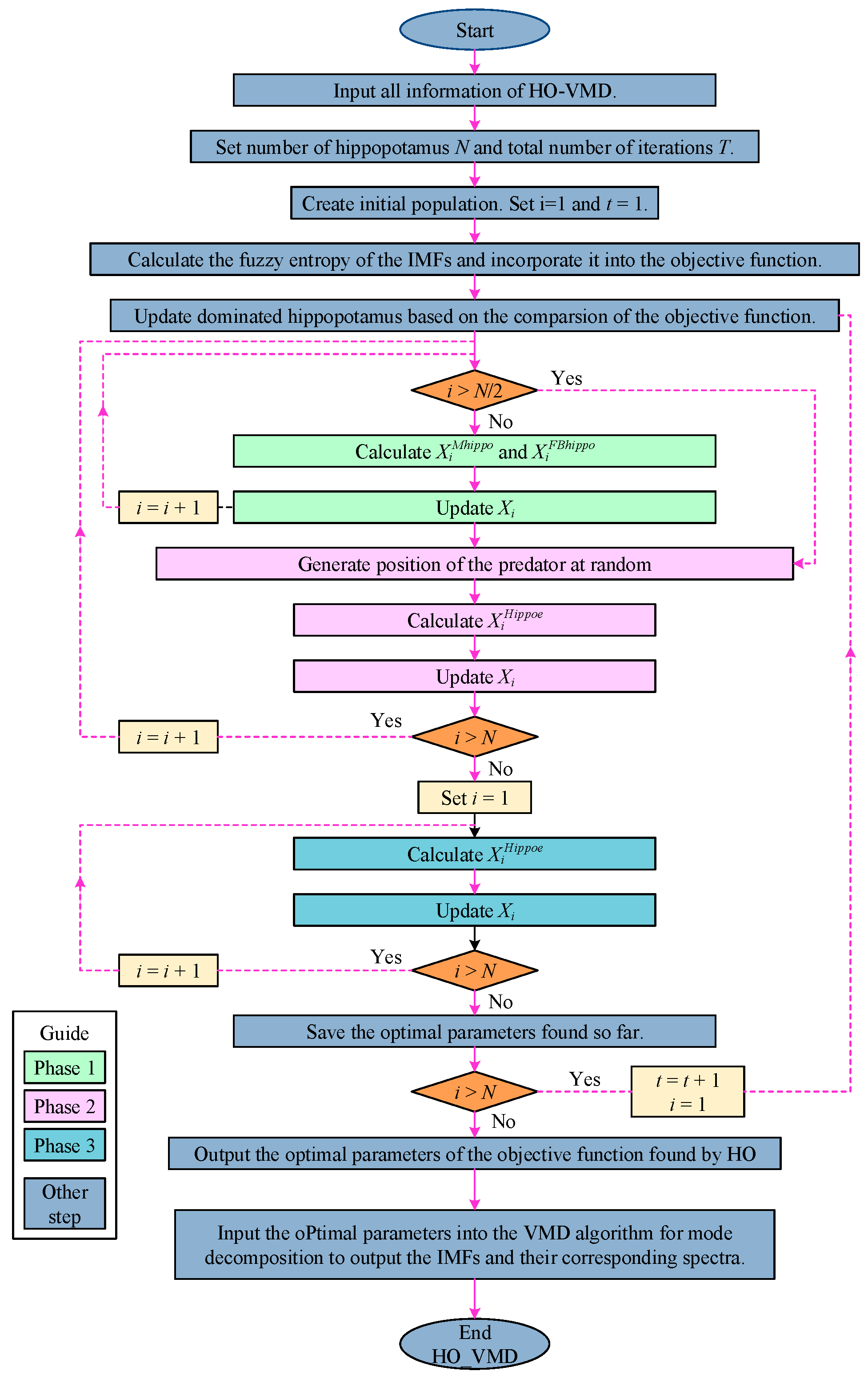
Figure 1. Flowchart of the HO-VMD algorithm.
Energies 17 05067 g001
Figure 2. Flowchart of the HO-VMD and SVD-RTlS-Prony algorithm.
Energies 17 05067 g002
Figure 3. Illustration of ideal signal and signal with noise. (a) Ideal oscillation signal diagram. (b) Oscillation signal diagram with added white noise.
Energies 17 05067 g003
Figure 4. HO-VMD iteration curve graph.
Energies 17 05067 g004
Figure 5. Signal and spectrum plots obtained from ideal signal after HO-VMD. (a) IMFs obtained from ideal signal after HO-VMD. (b) Spectra of IMFs obtained from ideal signal after HO-VMD.
Energies 17 05067 g005
Figure 6. HO-VMD-reconstructed signal and ideal signal.
Energies 17 05067 g006
Figure 7. HO-VMD reconstructed signal and Prony fitted signal.
Energies 17 05067 g007
Figure 8. Schematic diagram of DFIG wind farm grid connection via series-compensated line.
Energies 17 05067 g008
Figure 9. Wind farm output power graph.
Energies 17 05067 g009
Figure 10. Real-time monitoring results based on energy ratio graph. (a) Time-variation graph of the energy ratio. (b) Graph of shutdown triggered by energy ratio.
Energies 17 05067 g010
Figure 11. Signal and spectrum plots obtained from actual signal after HO-VMD. (a) IMFs obtained from actual signal after HO-VMD. (b) Spectra of IMFs obtained from actual signal after HO-VMD.
Energies 17 05067 g011
Figure 12. Comparison between actual data and HO-VMD denoised data.
Energies 17 05067 g012
Figure 13. Comparison between denoised signal and SVD-RTLS-Prony-fitted signal.
Energies 17 05067 g013
Table 1. Denoising results of EMD and VMD algorithms at different orders.
SNRMSE
3-order EMD3.25104,627.47
3-order VMD (α = 500)16.984439.01
5-order EMD11.7614,770.51
5-order VMD (α = 1000)15.126808.60
7-order EMD10.2920,685.75
7-order EMD (α = 2000)14.657593.49
Table 2. Identification results of ideal signal using SVD-RTLS-Prony.
ModeAmplitude Frequency Damping Factor Damping Ratio
1277.3615.600.41−0.41
2221.0732.40−0.180.09
3162.7847.600.26−0.09
Table 3. Identification results of actual signal using SVD-RTLS-Prony.
ModeAmplitude Frequency Damping Factor Damping Ratio
1269.44250.00−0.10100.00
234.26720.00−64.22100.00
318.6539.824.99−2.04
428.36243.17−106.356.94
Disclaimer/Publisher’s Note: The statements, opinions and data contained in all publications are solely those of the individual author(s) and contributor(s) and not of MDPI and/or the editor(s). MDPI and/or the editor(s) disclaim responsibility for any injury to people or property resulting from any ideas, methods, instructions or products referred to in the content.