Abstract
In order to change the centralized operation framework of the active distribution network with electric heating loads (EHLs), a distributed optimization method is proposed for the coordinated operation of the active distribution network with EHLs. Firstly, considering the thermal delay effect and heat loss of the thermal system, a centralized optimization operation model for active distribution networks with EHLs is established. Then, based on the centralized optimization operation model, it is rephrased as a standard sharing problem, and a distributed optimization operation model for the EHL active distribution network is established based on the alternating direction multiplier method (ADMM) solution. In the process of solving ADMM, dynamic step correction was further considered. By updating the steps during the iteration process, the number of iterations was reduced, and the convergence and computational efficiency of ADMM were improved. Finally, the effectiveness of the distributed coordinated operation method proposed in this paper was simulated and verified by constructing an IEEE33 distribution system. The results showed that the proposed distributed coordinated operation method has strong robustness to the randomness of the number of distributed units and parameters, and EHLs participating in coordinated operation can expand the consumption space of wind power and photovoltaic power, and improve the economic efficiency of system operation.
1. Introduction
The increasing proportion of new energy generation and the integration of multiple types of loads have had a serious impact on the safe and stable operation of the power grid [1,2]. Flexible loads in active distribution networks are balanced between supply and demand through demand response technology [3,4], maintaining the safe and stable operation of the system in the event of disturbances or faults in the power grid [5,6]. The current scheduling operation of active distribution networks mainly improves the system’s regulation ability by utilizing energy storage and flexible load demand response [7,8,9]. With the development of electric heating technology, EHLs have become a demand response resource with significant regulation ability on the load side [10]. EHLs mainly include two categories: space heating EHLs and domestic hot water EHLs [11]. Whether in European and American countries or China, space heating and domestic hot water production account for a large proportion of household energy consumption. In China, space heating accounts for 54% of household energy consumption and is the main source of household energy consumption. Hot water production accounts for 14% of household energy consumption, making it the third largest part of household energy consumption [12]. In developed countries in Europe and America, the proportion of space heating and domestic hot water production in household energy consumption is 80% and 60%, respectively [13].
EHLs belong to clean heating methods, which use electricity to heat electric heating conversion equipment for user heating during periods of relatively low electricity prices. Compared with the heating method of configuring heat storage devices and coal-fired boilers, using EHLs for heating has significant advantages. The configuration of heat storage devices in cogeneration only reduces the coupling characteristic of heat to electricity in cogeneration units and does not generate new load space for the consumption of new energy electricity [14]. The use of EHLs for heating can not only maintain the stability of heating, but also reduce costs through the adjustment of market electricity prices, expand the consumption space of new energy from the load side, and have a positive effect on peak shaving and valley filling of the power grid. However, the distribution of EHLs is relatively scattered, with a variety of types and significant differences, making it difficult for EHLs to participate in the coordinated operation of active distribution networks. Therefore, using distributed methods to solve the coordinated operation problem of active distribution networks containing EHLs is of great significance for achieving safe and efficient operation of new energy power systems.
The scheduling operation of traditional power systems adopts a centralized operation mode, which is achieved through traditional planning methods and intelligent optimization algorithms. In the centralized operation mode, each distributed unit reports parameters and boundary conditions to the central controller responsible for coordination [15], obtains the optimal solution for coordinated operation through the centralized solving method, and transmits it to each distributed device. Due to the presence of a large number of distributed devices in the active distribution network, the centralized operation mode requires a large communication capacity and storage space. Once a central single point of failure occurs, it will cause the system to crash [16]. In addition, the submission of parameter and constraint information will expose the privacy of distributed unit owners. Therefore, it is necessary to achieve coordinated and optimized operation of active distribution networks with EHLs by shifting the operating mode from centralized to distributed. At present, the main methods for solving distributed optimization include Alternating Direction Multiplier Method (ADMM), Analysis Objective Cascading Method (ATC), Near End Message Passing Method (PMP), Auxiliary Problem Principle (APP), Optimality Condition Decomposition Method (OCD), and so on. The ATC usually requires the establishment of a higher-level coordination center that can grasp some boundary information. PMP, APP, and OCD do not require a higher-level coordination center and only rely on various regions to jointly complete information transmission and optimization calculations. However, their convergence is relatively poor, and the optimization results obtained may not be ideal. ADMM has a natural decoupling structure and stable convergence performance and has been widely used in distributed optimization operations of energy systems [17,18,19]. Reference [20] conducted research on the coordinated operation of power and natural gas systems based on ADMM. A decentralized optimal power flow method is proposed in reference [21] to reduce the communication burden between multiple integrated energy systems. Reference [22] established a day-ahead optimization scheduling model for the integrated energy system of electricity and natural gas and used an improved ADMM solution model to obtain the minimum operating cost.
In the above references, the interaction between different energy systems is only coupled through gas turbine units or cogeneration units. However, at the level of active distribution networks with EHLs, the coupling of multi-vector energy may be more complex. This operation involves the collaborative optimization of different forms of energy, including electricity and heat. The central operator is responsible for managing this operation. Meanwhile, with the continuous increase in various coupling devices, there are more and more operational entities in active distribution networks with EHLs. Therefore, the original ADMM cannot be directly applied to active distribution networks with EHLs, and the interaction between energy demand and the power grid should be addressed. Meanwhile, as the scale of distributed units in the system increases, the central coordinator in the distributed framework is expected to incur more communication costs. In addition, with the increase in data exchange, communication failures have become increasingly common. Therefore, it is necessary to propose a distributed operation framework to reduce the communication pressure of the system and achieve coordinated operation of active distribution networks with EHLs. In order to address these issues, the contributions made in this article are as follows:
- (1)
- Considering the thermal delay effect and heat loss of the thermal system, the centralized optimization operation model of active distribution networks containing EHLs is formulated as a standard sharing problem, and a distributed optimization operation model of EHLs active distribution networks based on ADMM solution is established.
- (2)
- The iterative process is improved by dynamically updating the step, which results in fewer iterations and better convergence performance compared to the original ADMM. In addition, this method can not only obtain the optimal solution with the minimum number of iterations under normal operation but also obtain the optimal solution with the minimum number of iterations in the case of communication failures.
- (3)
- The effectiveness of the distributed coordinated operation method proposed in this paper was simulated and verified by constructing an IEEE33 distribution system. The results showed that the proposed distributed coordinated operation method has strong robustness to the randomness of the number of distributed units and parameters. Moreover, EHLs participating in coordinated operation can expand the consumption space of wind power and photovoltaic power, and improve the economic efficiency of system operation.
2. Centralized Optimal Operation Model for Active Distribution Networks with EHLs
Due to the existence of electrothermal coupling characteristics in active distribution networks with EHLs, in order to obtain a reliable operation plan, it is necessary to consider the thermal delay effect and heat loss of the thermal system when establishing an optimized operation model for active distribution networks with EHLs. Firstly, establish a centralized optimization operation model for active distribution networks with EHLs, and then rephrase it as a standard sharing problem based on the centralized optimization operation model. Finally, establish a distributed optimization operation model for active distribution networks with EHLs based on ADMM.
The centralized optimization of active distribution networks with EHLs is based on the power constraints of each distributed unit in the virtual power plant, taking into account the day-ahead load forecasting and real-time price, to achieve the minimum comprehensive operation cost of active distribution networks with EHLs.
2.1. Objective Function
The Equation (1) is shown as below:
where N is the total number of virtual power plants in the active distribution network. , , , and are the operating costs of conventional units, Cogeneration units, wind turbine units, photovoltaic generator units, and EHLs in virtual power plant i, respectively. is the cost of purchasing energy for virtual power plant i from other virtual power plants, that is, the cost of energy sharing.
where T is the total number of running periods. is the generating power of conventional units in virtual power plant i in period t. A represents the cost of changing the operating status of a conventional unit from static to operational during time t. is the operating status of conventional units in period t; and represent the operating and shutdown states, respectively. is the start-up cost for conventional units. is the power generation cost of conventional units in period t. , and are the generation cost coefficient of conventional units. and are the output of wind power and photovoltaic generator units of virtual power plant i in period t. and is the output maintenance cost coefficient of wind power and photovoltaic generator units in virtual power plant i. and are the energy sharing prices of the virtual power plant in the active distribution network, representing electric energy and thermal energy respectively. and are, respectively, the power received and provided by virtual power plant i for energy sharing in period t. and are respectively the heat received and provided by virtual power plant i for energy sharing in period t.
where , , , , and are the operating cost coefficients of cogeneration units in virtual power plant i. and are the electrical output and thermal output of cogeneration units in virtual power plant i in period t.
EHLs consider the thermal inertia and thermal delay effects of the thermal system while meeting user comfort and operational constraints, and fully tap into the regulatory potential of EHLs.
where, is the active power of EHLs in virtual power plant i in period t. is the compensation price for EHLs.
According to the Weber–Fechner law, a more effective and reasonable pricing method is determined, specifically expressed as:
where the compensation price of EHLs in the power system is related to the electricity price , while the compensation price of EHLs in the thermal system is related to the heating price; is the compensation coefficient of electrothermal coupled EHLs, taken as 0.5. The constant K is generally taken as 1 based on the experience of Weber-Fechner law.
According to the coordinated operation requirements of the system, the actual controlled EHLs during the t period can be expressed as follows in Equation (4):
where is the maximum regulating power of EHLs in virtual power plant i. is the regulation rate.
For rebound loads, there is currently no precise mathematical model to describe them, and a three-stage autoregressive model is generally used to fit them as follows:
where is the rebound load of EHLs in virtual power plant i in period t. , and are the regulated power of EHLs in period t-1, t-2, and t-3, respectively. , and are the rebound coefficients.
2.2. Constraints
2.2.1. Power Balance Constraints
The Equation (8) is shown as below:
where is the load of virtual power plant i in period t.
2.2.2. Thermal Power Balance Constraints Considering Thermal Loss and Thermal Delay Effects
The Equations (9) and (10) are shown as below:
where is the thermal load of virtual power plant i in period t. and are the heating capacity of cogeneration units and EHLs in virtual power plant i in time period t, respectively. is the heat loss when virtual power plant i supplies heat to the user in time period t. TD is the delay time of heat transfer, which depends on the parameters of heat pipes. is the heat loss coefficient of the thermal system. Constraint (9) considers the heat loss and thermal delay effects of the thermal system.
2.2.3. Conventional Unit Operation Constraints
The Equation (11) is shown as below:
where and are the upper and lower limits of conventional unit output.
where and , respectively, represent the continuous start and stop times of conventional units. and are the minimum continuous start and stop times for conventional units. Equation (12) represents the minimum start and stop time constraint for conventional units.
2.2.4. Operation Constraints of Cogeneration Units
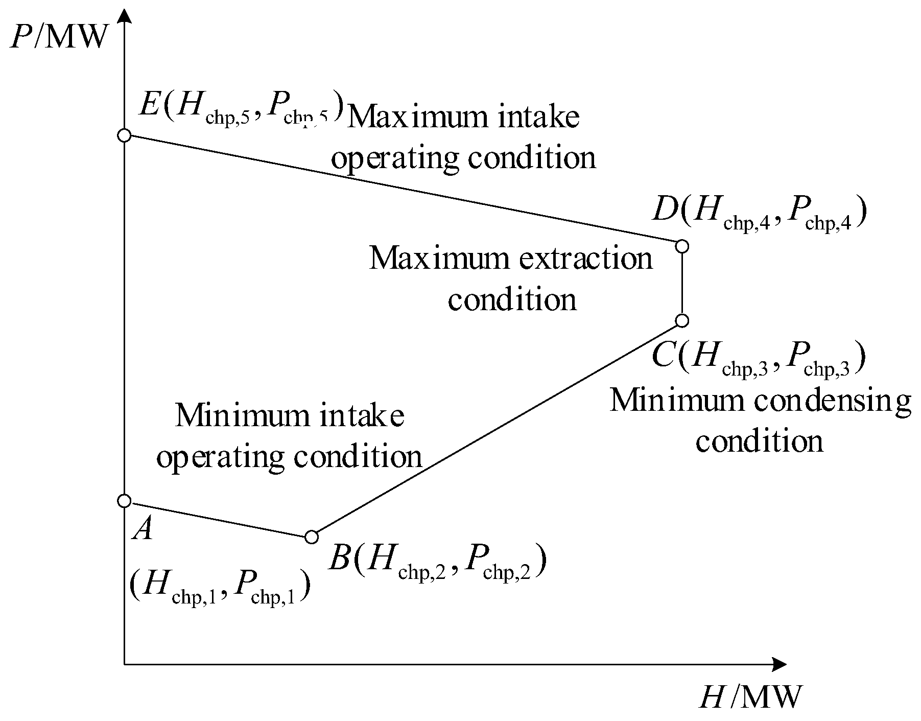
The feasible range of output of cogeneration units is shown in Figure 1.

Figure 1.
Cogeneration output feasibility region.
The operation of cogeneration units shall be included in the feasible range of output:
where and are the extreme points of cogeneration power and thermal output range, respectively. is the output coefficient of the extreme point. is the set of vertices in the feasible region of output.
2.2.5. Operational Constraints for Wind and Photovoltaic Power Generation
The Equations (14) and (15) are shown as below:
where and , respectively, represent the predicted power of wind and photovoltaic power generation.
2.2.6. EHLs Operational Constraints
The Equation (16) is shown as below:
where and are, respectively, the minimum and maximum controlled quantities of EHLs participating in regulation in virtual power plant i in period t. is the state variable of EHLs. indicates that they are in a controlled state and indicates that they are not controlled. Equation (16) represents the controlled quantity constraint of EHLs.
where and are the minimum and maximum interruptible duration of EHLs participating in regulation. is the maximum number of actions required for EHLs to participate in regulation. Equations (17) and (18) represent the minimum interruptible duration constraint for EHLs. Equation (19) represents the maximum interruptible duration constraint for EHLs. Equation (20) represents the number of interruption constraints for EHLs.
2.2.7. Energy Sharing Constraints
The Equations (21) and (22) are shown as below:
where and are the maximum electric power received and provided by virtual power plant i, respectively. and are the 0-1 state variables for receiving and providing electric power for virtual power plant i, respectively. and are the maximum thermal power received and provided for virtual power plant i, respectively. and are the 0–1 state variables for receiving and providing thermal power for virtual power plant i, respectively.
3. Distributed Optimal Operation Model for Active Distribution Networks with EHLs
The centralized optimal operation model requires all Virtual power plants to directly provide trade secret data. In most cases, virtual power plants participating in system operation may belong to different interest groups, and it is difficult to fully realize information sharing in actual operation. Directly providing data will cause data privacy disclosure. However, ADMM is used to solve the optimal operation model for active distribution networks with EHLs in a distributed manner, then the commercial privacy data of each virtual power plant can be protected. In addition, the SOCP-based AC power flow model shown in Equations (24)–(31) is used to simulate active distribution networks with EHLs. To address the above issues, based on the ADMM, the centralized optimization operation model for active distribution networks with EHLs is rephrased as a standard sharing problem, as shown in Equations (23)–(36).
where I is the set of nodes in the active distribution network. I/N refers to the set of nodes excluding those connected to the virtual power plant. M is the collection of distribution lines. is the square amplitude of the current of the distribution line (i, j) in period t. is the squared amplitude of the voltage at node i in period t. and , respectively, refer to the resistance and reactance of distribution lines (i, j). is the power factor of the virtual power plant. is the net power output of virtual power plant i in period t. is the net thermal output of virtual power plant i in period t. Constraints (24) and (25) represent the active and reactive power balance of each node, respectively. Constraint (26) describes the voltage drop of the distribution line. Constraint (27) provides second-order cone relaxation for nonlinear AC power flow constraints [23]. Constraint (28) represents the balance of active and reactive power at nodes of the Common Coupling Point (PCC). Constraints (29), (30), and (31) represent power factor limitations, voltage squared amplitude limitations of nodes, and current squared amplitude limitations of distribution lines, respectively.
In order to express the centralized optimization operation model of active distribution networks with EHLs as a standard sharing problem [24], two auxiliary variables and are defined, as shown in Equation (34):
According to the defined auxiliary variables, the augmented Lagrange function of the model shown in Equations (23)–(34) can be expressed as:
where , . and are Lagrange multipliers. and are penalty coefficients.
Combine the linear term and the quadratic term, make , , and express the augmented Lagrange function (35) as a scaling form:
where and are scaled dual variables.
4. Distributed Solution Based on Dynamic Step Correction ADMM
In order to protect the privacy of the Virtual power plant during the operation of active distribution networks with EHLs, ADMM is used to solve the optimal operation model of active distribution networks with EHLs in a distributed manner. Since the step size will significantly affect the rate of convergence of ADMM, the dynamic step size modification is further considered on the basis of the original ADMM to improve the convergence performance of the algorithm.
4.1. Implementation of ADMM
The updates of each variable are shown in Equations (37)–(39):
For the convenience of analysis, let:
The iteration stopping standard is defined as the original residual and dual residual being less than the set tolerance. Specifically, it is determined whether the ADMM iteration has stopped based on the stopping standard shown in Equation (41).
The solving steps of the original ADMM are shown in Algorithm 1.
| Algorithm 1. ADMM-based distributed optimization |
| Input: Forecast electric load , forecast thermal load , wind power forecast output , photovoltaic forecast output , Lagrange multiplier and , penalty coefficient and , tolerance parameter and , energy price and equipment operation parameter Output: Minimum operating cost of active distribution network with EHLs |
| Step 1: Initialize , , , , , iteration number k = 1. Step 2: Establish an optimization operation model for active distribution networks with EHLs, including optimization objective functions and constraint conditions. Step 3: Parallel optimization and solution of various variables in the model. Step 4: According to Equations (37)–(39), iteratively update variables and , auxiliary variables and , and dual variables and . Step 5: Update iteration number k = k + 1. Step 6: According to Equation (41), determine whether the stop condition is met. If the stop condition is met, the iteration stops. Otherwise, return to Step3 for repeated calculations. |
4.2. Dynamic Step Correction of ADMM
The step size will have a significant impact on the rate of convergence of ADMM [24], while the step size of the original ADMM is fixed, and the algorithm performance will deteriorate during the iteration process. Therefore, a two-stage dynamic step size correction method is adopted to improve the convergence performance of ADMM.
Stage 1: Calculate the changes in the original residual and dual residual values during each iteration process, as shown in Equation (42). If the change in the minimum values of the original and dual residuals is greater than the set value (such as ), the step size remains unchanged because the current step size reduces the original and dual residuals. Otherwise, the current step size will worsen the convergence of the algorithm. At this time, the step size needs to be updated at Stage 2.
Stage 2: Update the step based on the current values of the original and dual residuals, as shown in Equation (43). If the original residual is much greater than the dual residual, it will increase the step size and result in serious penalties for violating the original feasibility. If the dual residual is much greater than the original residual, then the dual feasibility converges and the step size will decrease. At this time, the convergence of original feasibility and dual feasibility can alternate and balance.
The ADMM for dynamic step size correction is shown in Algorithm 2.
| Algorithm 2. ADMM based on dynamic step size correction |
| Step 1: Set residual variation value ; Step 2: for k Calculate and according to Equation (42) if min else Update according to Equation (43) end is sent to Algorithm 1 for step3 update Step 3: end |
5. Simulation and Analysis
5.1. Example Setting
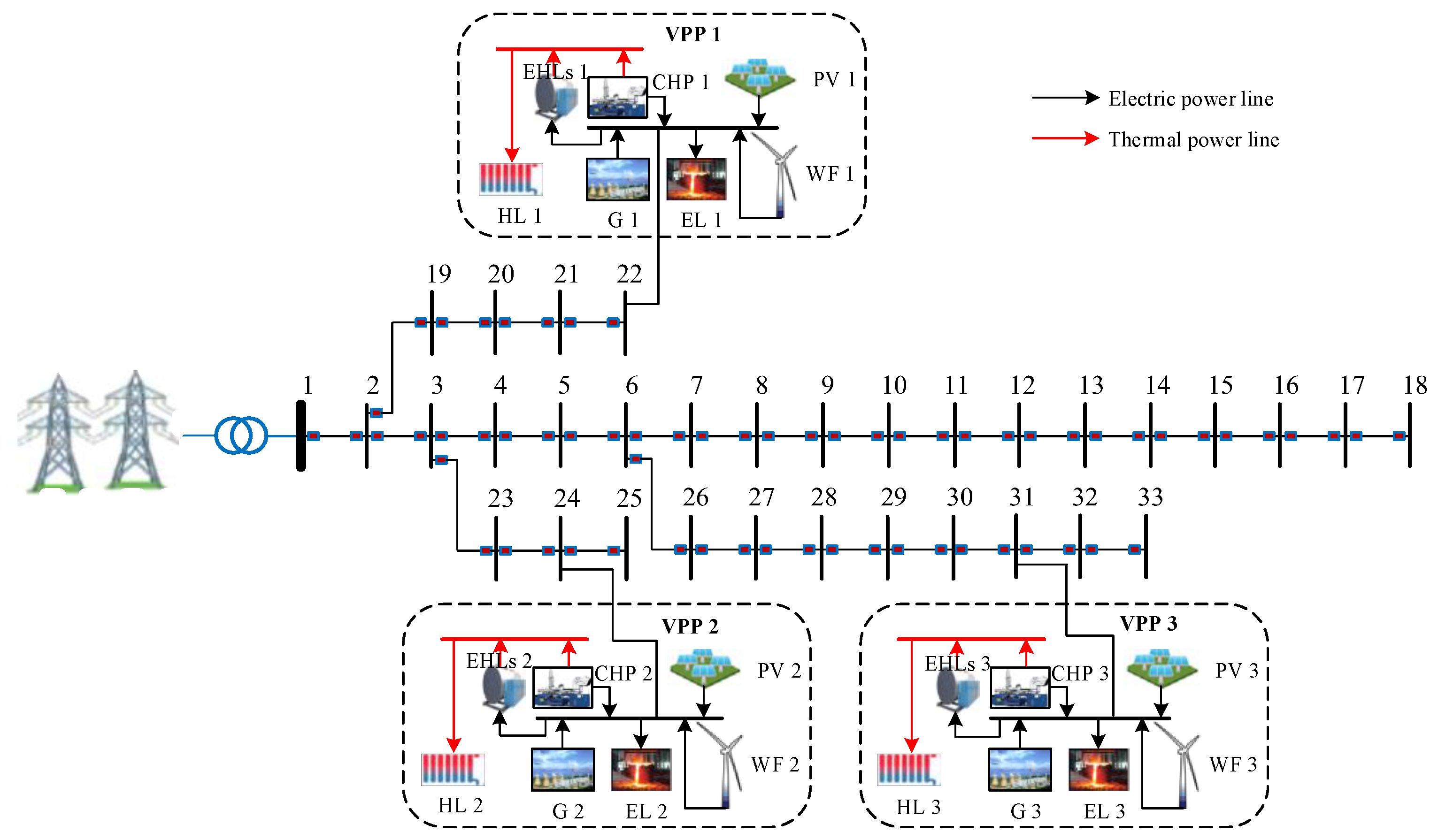
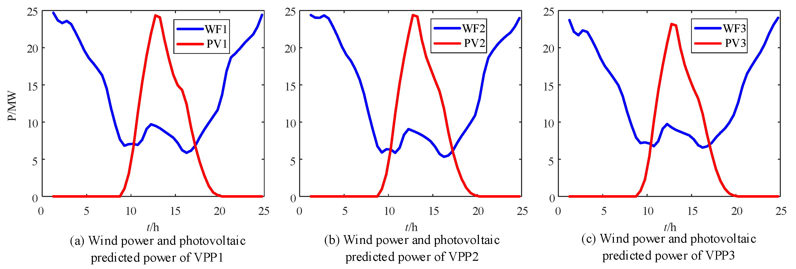
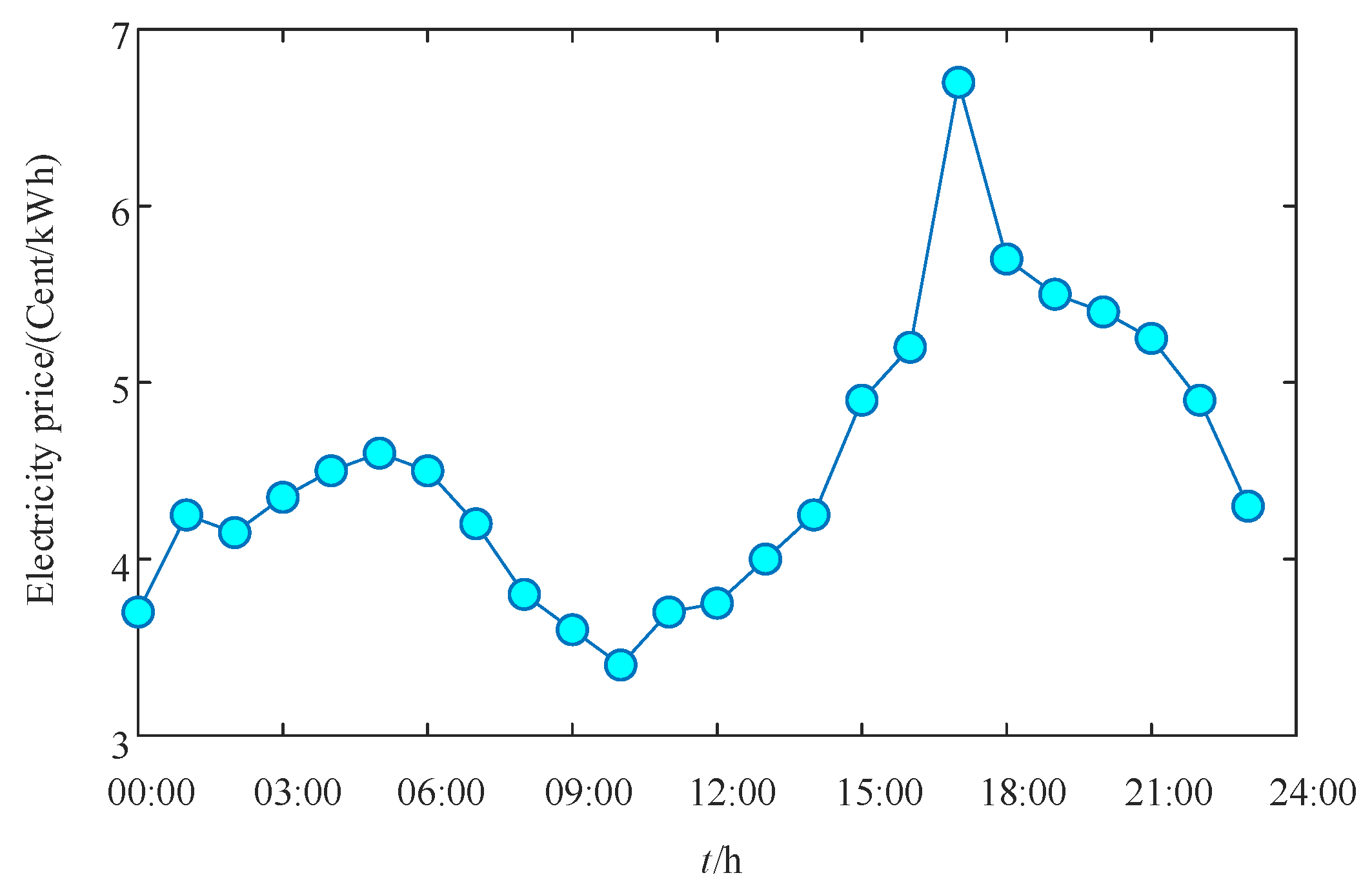
To verify the effectiveness of the distributed coordination and optimization operation method for active distribution networks with EHLs based on ADMM, an IEEE33 distribution system as shown in Figure 2 was constructed for simulation verification. A total of 21 distributed units are aggregated into the active distribution network through three virtual power plants (VPP1, VPP2, VPP3). The parameters of conventional units (G1, G2, G3), cogeneration units (CHP1, CHP2, CHP3), wind turbines (WF1, WF2, WF3), photovoltaic power generation (PV1, PV2, PV3), and electrical heating loads (EHLs1, EHLs2, EHLs3) in distributed units are shown in Table 1, Table 2, Table 3, Table 4 and Table 5, and the predicted power of wind and photovoltaic is shown in Figure 3. The shared electrical power of each virtual power plant is limited to 28 MW, and the shared thermal power is limited to 5 MW. The electricity sharing price between virtual power plants is shown in Figure 4, and the heat sharing price is 0.06 $/kW·h.

Figure 2.
IEEE33 distribution system.

Table 1.
Conventional unit operating parameters.
Table 2.
Output range of cogeneration unit.
Table 3.
Operating parameters of cogeneration unit.
Table 4.
Wind power and photovoltaic operating parameters.
Table 5.
EHLs operating parameters.
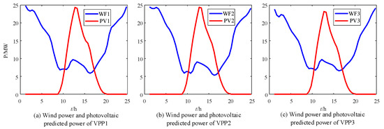
Figure 3.
Wind power and photovoltaic predicted power.
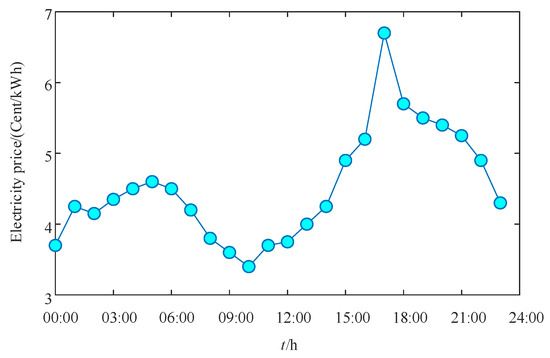
Figure 4.
Electricity sharing price between virtual power plants.
5.2. Algorithm Performance Analysis
To verify the effectiveness of the proposed distributed coordinated operation method for active distribution networks with EHLs based on dynamic step size correction ADMM (represented as A1), this method was compared with the original ADMM algorithm (represented as A2) in reference [25] and the automatically adjusted step size ADMM algorithm (represented as A3) in reference [19], as shown in Table 6.
Table 6.
Operating results of different methods.
It can be seen from Table 6 that A1 always has the fastest rate of convergence under different convergence precision, the operating cost remains stable, and the economy is optimal. Taking convergence accuracy as an example, the A2 iteration converges 162 times, the A3 iteration converges 79 times while the A1 iteration only converges 57 times, which is significantly less than other methods. Obviously, the proposed method helps to improve the convergence of the algorithm. In addition, for A2 and A3, as the convergence accuracy decreases, the operating results gradually deteriorate. This is because their convergence is formed as each distributed unit evolves independently, while the exit condition is only based on overall error. At the same time, the intermediate results summarized by the virtual power plant layer shield the cost parameters of each distributed unit in each iteration.
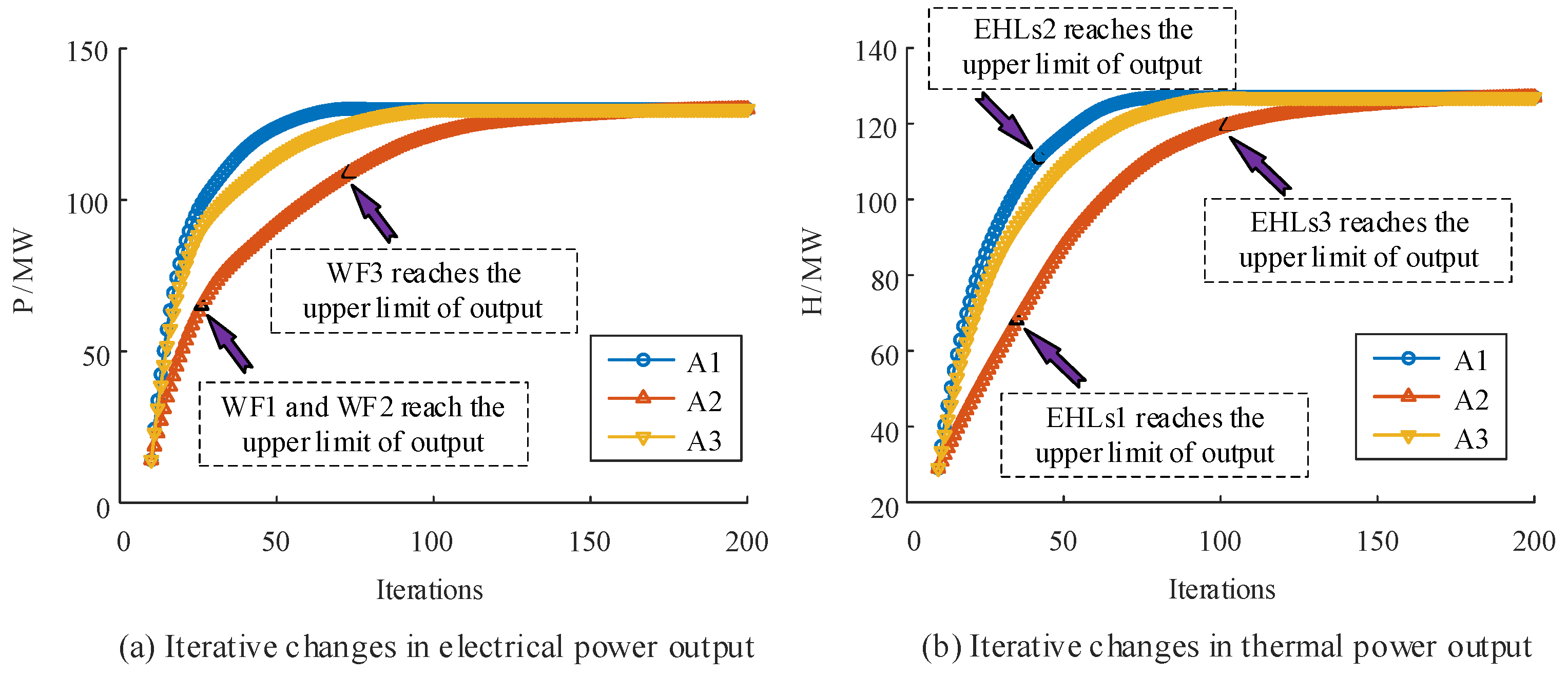
To achieve convergence accuracy , the simulation analysis shows the convergence characteristics of power output, as shown in Figure 5 and Figure 6.
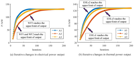
Figure 5.
Convergence characteristics under normal communication.
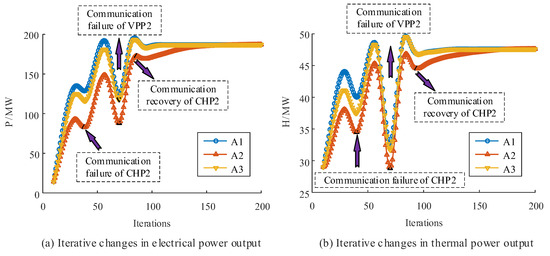
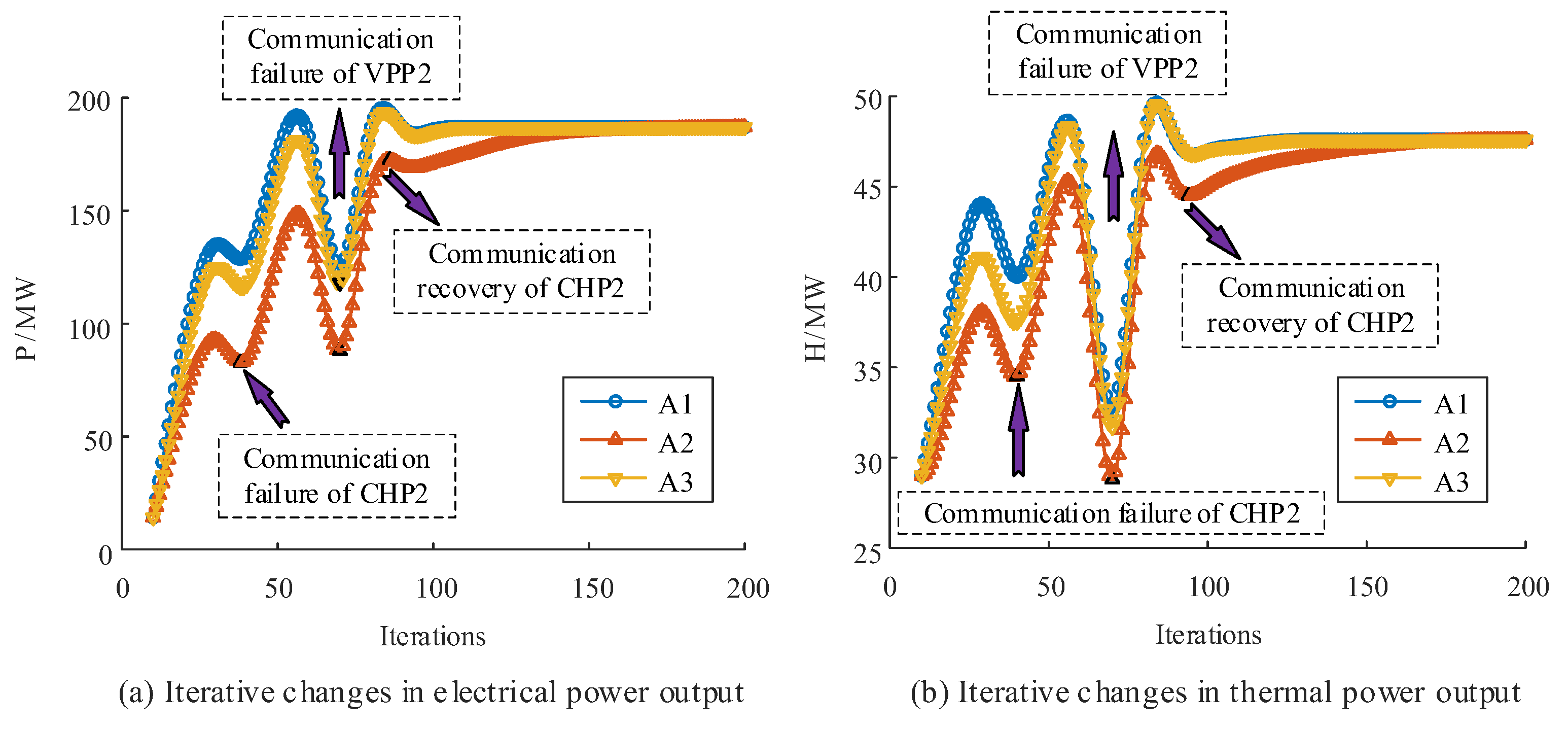
Figure 6.
Convergence characteristics under communication failure.
Figure 5 shows the changes in the power output and thermal power output of the device during normal communication at 24:00 with the number of iterations. The number of iterations required for A2 and A3 power output convergence is 196 and 93, respectively, while A1 power output only needs 69 iterations to converge, which is significantly superior to the other two methods. The dynamic correction step is generated by dynamically adjusting the online distributed units from bottom to top, ensuring convergence speed. In the system economy operation, compared with conventional power generation units, wind power, and photovoltaic operation costs are lower, and the output of distributed units such as WF1, WF2, and WF3 will reach the upper limit during the iteration process.
In addition, verify the optimization effect of dynamic step size correction ADMM under communication faults. Figure 6 shows the variation of electrical and thermal power output with the number of iterations under communication faults at 12:00 pm. Assuming that there is a communication failure between CHP2 and virtual power plant 3 during the iteration process, distributed optimization is carried out based on the dynamic correction strategy proposed in the previous section, that is, each distributed unit and virtual power plant are optimized using the latest information obtained. The dynamic correction step size can ensure that new stable operating points can be quickly reached in the event of communication connection failures in distributed units or virtual power plants. Compared with normal situations, the number of iterations under communication faults has increased, but as shown in Figure 6, the proposed method can obtain the optimal solution with the minimum number of iterations under communication faults, still outperforming other methods.
5.3. The Impact of Distributed Unit Randomness
In the three-layer distributed coordinated operation architecture, EHLs, and other distributed units in the active distribution network are widely distributed, with strong spatiotemporal dispersion and differences, which may lead to changes in the number and parameters of the underlying distributed units. Therefore, the solution speed and efficiency should have strong robustness to the randomness of the number of distributed units and parameters.
The distributed coordinated operation of active distribution networks with EHLs needs to meet the constraints of supply and demand balance and the constraints of distributed unit operation, specifically expressed as:
where is the output of distributed unit i, is the system load demand, and is the upper and lower limits of the output of distributed unit i.
According to the constraints of supply and demand balance and distributed unit operation, a necessary condition that the system’s economic operation must meet is:
Define the depth of distributed unit operation based on the above conditions (represented as 0 < m < 1), and have
In order to compare the influence of the number of distributed units on the algorithm convergence, assume that the parameters of different distributed units are randomly distributed in some intervals, generate a certain number of distributed units randomly from them, and form the randomness of virtual power plant simulation distributed units.
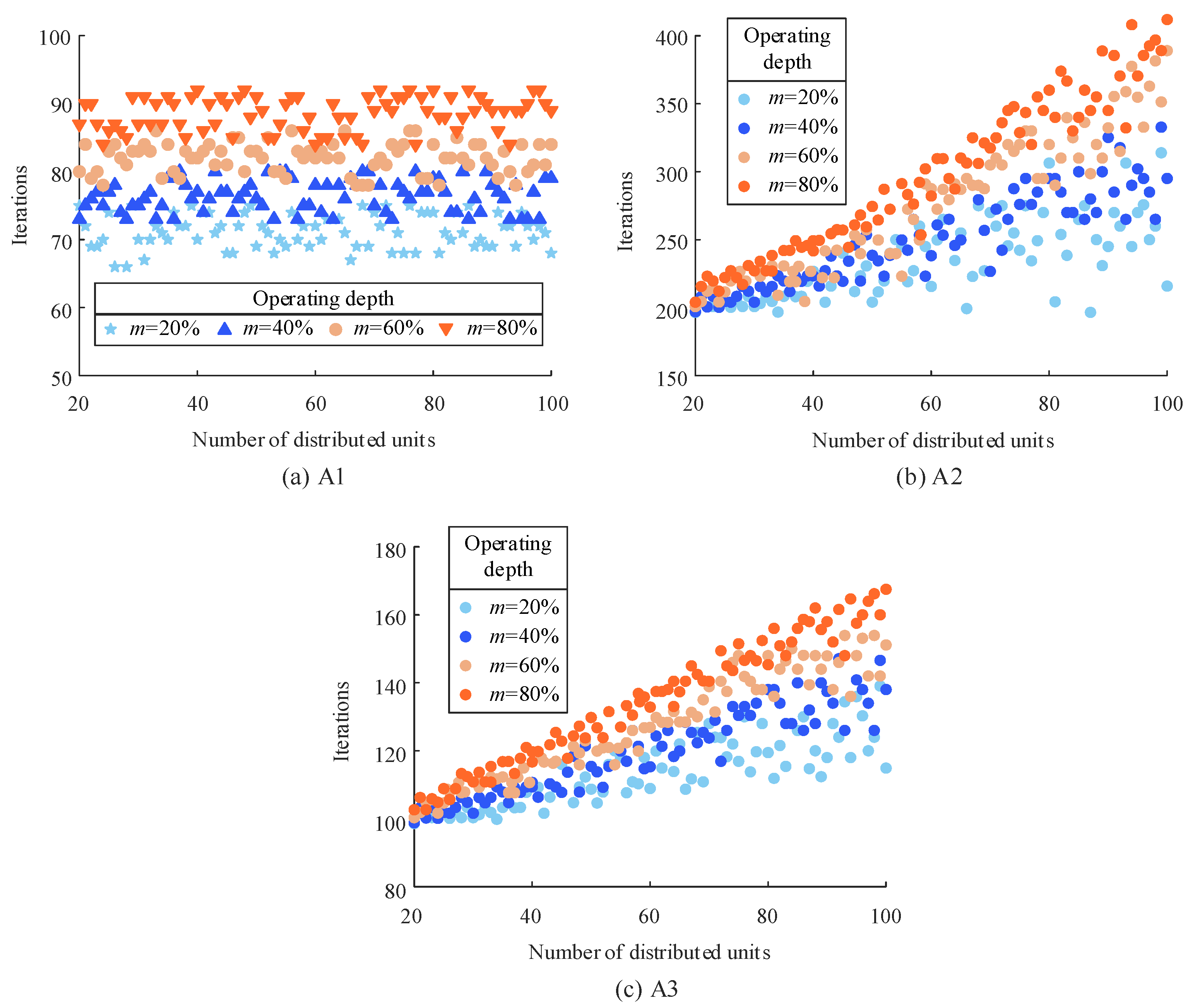
Figure 7 shows the convergence of the three methods at different operating depths when the number of distributed units changes from 20 to 100. It can be seen that the number of iterations for A2 and A3 is greatly affected by the number of distributed units. The number of iterations for A2 is approximately exponential with the number of distributed units, requiring hundreds of iterations to converge. For A3, the number of iterations is approximately linearly increasing with the number of distributed units, requiring over a hundred iterations to converge. The number of iterations for A1 is almost unaffected by the number of distributed units, and for a certain m, it can converge with only a few dozen iterations. This is because the step size of A1 is dynamically modified, which is updated from bottom to top based on the response of the underlying distributed units.
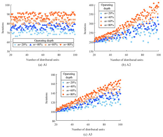
Figure 7.
The impact of the number of distributed units on the number of iterations under different methods.
5.4. Distributed Coordinated Operation Results of the Active Distribution Network with EHLs
The distributed coordinated operation of active distribution networks with EHLs takes into account both thermal delay effects, thermal losses, and EHL regulation. In order to analyze the advantages of the distributed coordinated operation strategy in this paper, four operation strategies are set based on whether the thermal delay effect and heat loss of the heating system are considered during coordinated operation, and whether EHLs participate in the operation. Strategy A: The distributed coordinated operation of the system does not consider the thermal delay effect and heat loss, nor does it consider EHL regulation. Strategy B: The distributed coordinated operation of the system only considers the thermal delay effect and heat loss, without considering EHL regulation. Strategy C: The distributed coordinated operation of the system does not consider the thermal delay effect and heat loss, only EHLs regulation. Strategy D: The distributed and coordinated operation of the system takes into account the thermal delay effect, heat loss, and EHL regulation. Table 7 compares the four operating strategies in terms of system operation economy. Table 8 compares the wind abandonment situation under four operating strategies, and Table 9 compares the photovoltaic abandonment situation under four operating strategies.
Table 7.
The four operating strategies in terms of system operation economy.
Table 8.
The wind abandonment situation under four operating strategies.
Table 9.
The photovoltaic abandonment situation under four operating strategies.
It can be seen from Table 7, Table 8 and Table 9 that, compared with Strategy A, individually considering the thermal delay effect and heat loss of the heating system (Strategy B) and EHLs regulation (Strategy C) can both reduce the system operating costs and waste wind and solar energy to a certain extent. Compared with strategy D, the system operation economy and the potential of wind and solar energy consumption have not been fully released. Under the distributed and coordinated operation of active distribution networks with EHLs (Strategy D), the system has the lowest operating cost, only 2.3071105 $, and the wind and photovoltaic abandonment rates have further decreased to 6.7% and 5.1%.
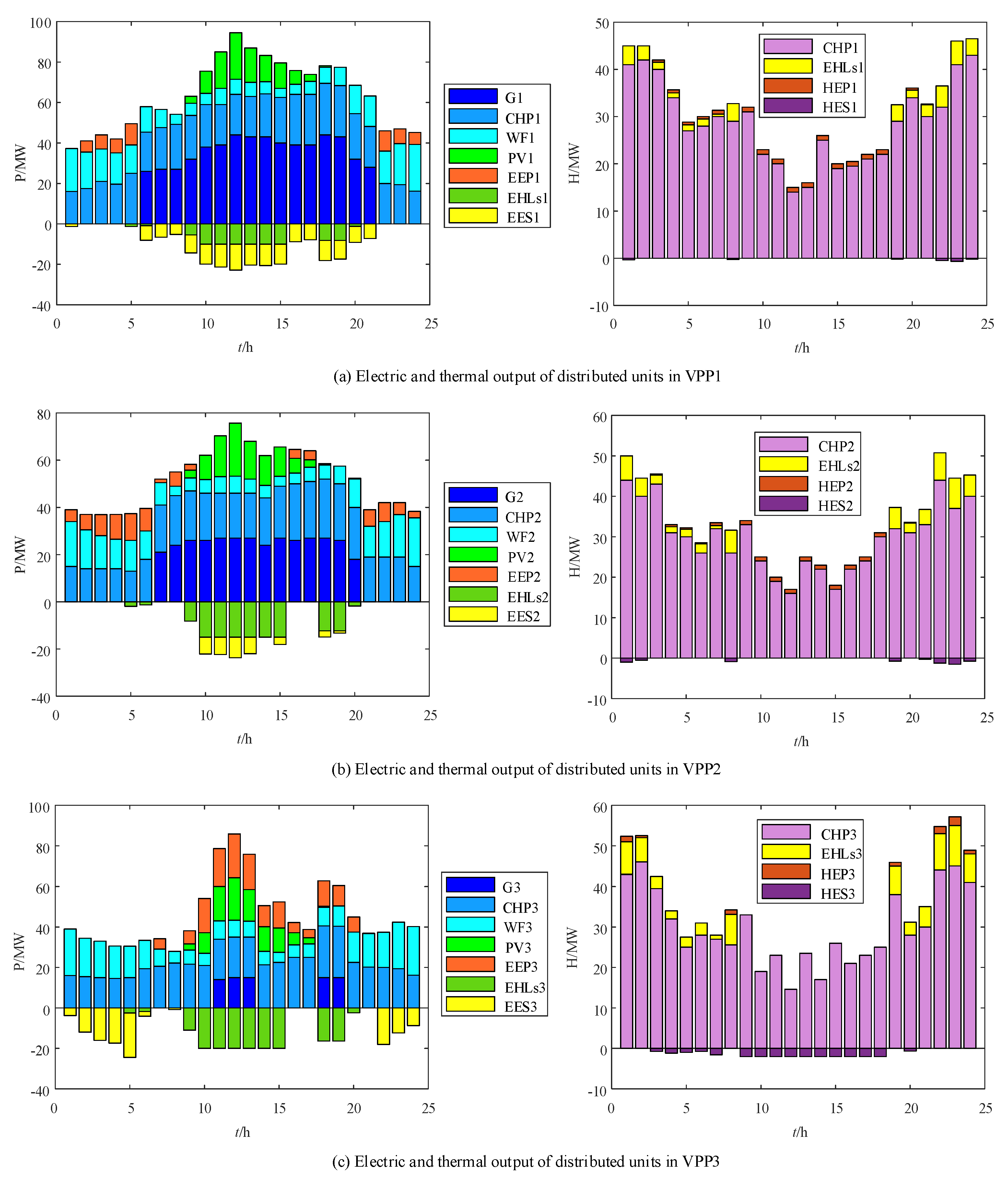
Figure 8 shows the coordinated operation results of various distributed units in the active distribution network with EHLs.
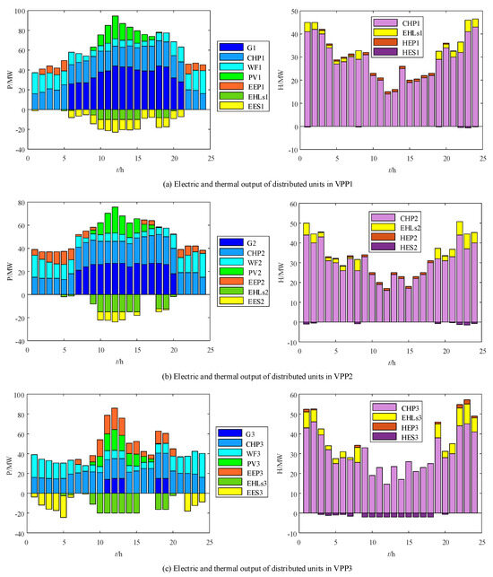
Figure 8.
Distributed coordinated operation results of the active distribution network with EHLs.
Take virtual power plant 1 as an example to analyze the results. According to the power optimization operation results in Figure 8a, the power demand of virtual power plant 1 in the daytime is mainly met by G1, CHP1, and PV1, and the power demand of virtual power plant 1 at night is mainly met by CHP1, and WF1. This is because during the day from 11:00 to 15:00, there is sufficient sunlight, and PV1 is in the period of high power generation. At night from 20:00 to 05:00, the wind speed is high, and WF1’s power generation significantly increases. In order to provide space for wind power consumption, G1 is in a shutdown state from 22:00 to 05:00. In addition, CHP1 is running all day due to providing heat to users. Virtual power plant 1 energy sharing receives 78.28 MW·h of electric energy and provides 322.80 MW·h. According to the thermal optimization operation results in Figure 8a, the thermal demand of virtual power plant 1 is mainly provided by CHP1 in the daytime, while it is in the peak heating period at night, and the thermal demand of Virtual power plant 1 is mainly provided by CHP1 and EHLs1. The heat energy received by virtual power plant 1 energy sharing is 13.72 MW·h, and the heat energy provided is 2.08 MW·h. Analysis shows that the active distribution network with EHLs achieves a distributed collaborative supply of electricity and heat energy.
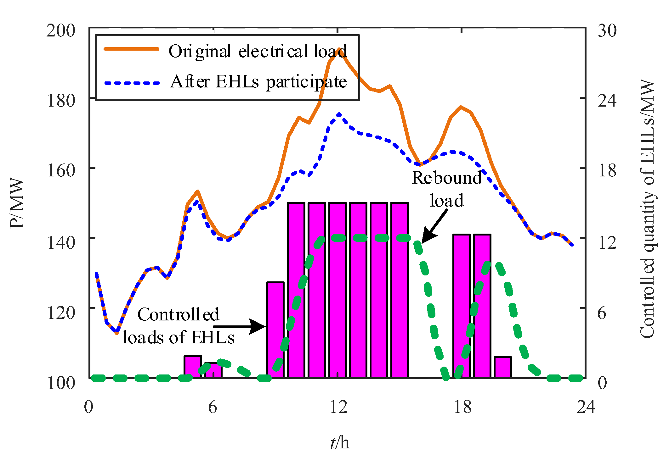
The power load, EHLs controlled quantity, and rebound load are shown in Figure 9.
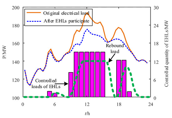
Figure 9.
Power load and EHLs controlled quantity.
From Figure 9, it can be seen that the trend of rebound load is consistent with the controlled quantity of EHLs, but the rebound load is relatively delayed in time compared to the controlled quantity of EHLs, and the peak of rebound load is also smaller compared to the controlled quantity of EHLs. Due to the peak power load during the day, EHLs are mainly controlled during the day. During the controlled period of EHLs, the peak value of the power load significantly decreases, reflecting the role of EHLs control in energy conservation and emission reduction of the power system.
The thermal load and the controlled quantities of EHLs in the thermal system are shown in Figure 10.
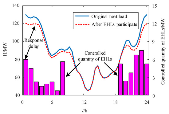
Figure 10.
Thermal load and EHLs controlled quantity.
From Figure 10, it can be seen that compared to the response time of the heat load, the control time of EHLs is advanced by one hour, while the response time of the heat load is relatively delayed by one hour. Due to the peak heat load period at night, the controlled period of EHLs is mainly located at night. During the controlled period of EHLs, the peak value of thermal load significantly decreases, reflecting the role of EHLs control in energy conservation and emission reduction of the thermal system.
6. Conclusions
To solve the problem of coordinated operation of large-scale distributed units in active distribution networks with EHLs, a distributed coordinated operation method for active distribution networks with EHLs based on dynamic step correction ADMM is proposed. The effectiveness of the proposed method was verified through simulation, and the following conclusions were obtained:
- (1)
- In the process of solving ADMM, considering dynamic step correction can reduce the number of iterations and improve the convergence and computational efficiency of ADMM.
- (2)
- The proposed distributed coordinated operation method has strong robustness to the randomness of the number of distributed units and parameters.
- (3)
- After EHLs participate in coordinated operation, they can expand the consumption space of wind and photovoltaic power, improve the economic efficiency of system operation, and during the controlled period of EHLs, the peak values of electricity and heat loads significantly decrease, reflecting the energy-saving and emission reduction effect of EHLs on the system.
Author Contributions
Conceptualization, S.L.; methodology and data curation, S.L. and G.B.; model establishment, S.L.; data analysis, S.L. and G.B.; writing—original draft preparation, S.L.; project administration and supervision, Y.H.; visualization, G.B. and Y.H. All authors have read and agreed to the published version of the manuscript.
Funding
This research was supported by the Science and Technology Project of State Grid Corporation of China under Grant (No. 52272220002T); Sichuan Provincial key research and development program of China (No. 2022YFG0123); and in part by Central Government Funds for Guiding Local Scientific and Technological Development of China (No. 2021ZYD0042).
Data Availability Statement
Data are contained within the article.
Conflicts of Interest
This paper is completed by the author and our team without any plagiarism. We declare that we do not have any commercial or associative interest that represents a conflict of interest in connection with the work submitted.
References
- Dehnavi, G.; Ginn, H.L. Distributed load sharing among converters in an autonomous microgrid including PV and wind power units. IEEE Trans. Smart Grid 2019, 10, 4289–4298. [Google Scholar] [CrossRef]
- Liu, J.; Cheng, H.Z.; Zeng, P.L.; Yao, L.Z. Rapid assessment of maximum distributed generation output based on security distance for interconnected distribution networks. Int. J. Electr. Power Energy Syst. 2018, 101, 13–24. [Google Scholar] [CrossRef]
- Wu, D.; Lian, J.; Sun, Y.; Yang, T.; Hansen, J. Hierarchical control framework for integrated coordination between distributed energy resources and demand response. Electr. Power Syst. Res. 2017, 150, 45–54. [Google Scholar] [CrossRef]
- Albadi, M.H.; El-Saadany, E.F. A summary of demand response in electricity markets. Electr. Power Syst. Res. 2008, 78, 1989–1996. [Google Scholar] [CrossRef]
- Yang, J.; Yuan, W.B.; Sun, Y.; Han, H.; Hou, X.C.; Guerrero, J.M. A novel quasi-master–slave control frame for PV-storage independent microgrid. Int. J. Electr. Power Energy Syst. 2018, 97, 262–274. [Google Scholar] [CrossRef]
- Li, P.; Wang, Z.X.; Wang, N.; Yang, W.H.; Li, M.Z.; Zhou, X.C. Stochastic robust optimal operation of community integrated energy system based on integrated demand response. Int. J. Electr. Power Energy Syst. 2021, 128, 106735. [Google Scholar] [CrossRef]
- Huang, W.J.; Zhang, X.; Li, K.P.; Zhang, N.; Strbac, G.; Kang, C.Q. Resilience oriented planning of urban multi-energy systems with generalized energy storage sources. IEEE Trans. Power Syst. 2022, 37, 2906–2918. [Google Scholar] [CrossRef]
- Masrur, H.; Shafie-Khah, M.; Hossain, M.J.; Senjyu, T. Multi-energy microgrids incorporating EV integration: Optimal design and resilient operation. IEEE Trans. Smart Grid 2022, 13, 3508–3518. [Google Scholar] [CrossRef]
- Seyedyazdi, M.; Mohammadi, M.; Farjah, E. A combined driver-station interactive algorithm for a maximum mutual interest in charging market. IEEE Trans. Intell. Transp. Syst. 2020, 21, 2534–2544. [Google Scholar] [CrossRef]
- Huang, X.Z.; Xu, Z.F.; Sun, Y.; Xue, Y.L.; Wang, Z.; Liu, Z.J. Heat and power load dispatching considering energy storage of district heating system and electric boilers. J. Mod. Power Syst. Clean Energy 2018, 5, 992–1003. [Google Scholar] [CrossRef]
- Wang, J.D.; Liu, J.X.; Li, C.H.; Zhou, Y.; Wu, J.Z. Optimal scheduling of gas and electricity consumption in a smart home with a hybrid gas boiler and electric heating system. Energy 2020, 204, 17951. [Google Scholar] [CrossRef]
- Zheng, X.Y.; Wei, C.; Qin, P.; Guo, J.; Yu, Y.H.; Song, F. Characteristics of residential energy consumption in China: Findings from a household survey. Energy Policy 2014, 75, 126–135. [Google Scholar] [CrossRef]
- International Energy Agency (IEA). Energy Balances of OECD Countries 2014; International Energy Agency: Paris, France, 2014. [Google Scholar]
- Chen, X.Y.; Kang, C.Q.; O’Malley, M.; Xia, Q.; Bai, J.H.; Liu, C. Increasing the flexibility of combined heat and power for wind power integration in China: Modeling and implications. IEEE Trans. Power Syst. 2015, 30, 1848–1857. [Google Scholar] [CrossRef]
- Chen, C.Y.; Chen, Y.; Zhao, J.B.; Zhang, K.F.; Ni, M.; Ren, B. Data-driven resilient automatic generation control against false data injection attacks. IEEE Trans. Industr. Inform. 2021, 17, 8092–8101. [Google Scholar] [CrossRef]
- Yu, X.; Xue, Y. Smart grids: A cyber–physical systems perspective. Proc. IEEE 2016, 104, 1058–1070. [Google Scholar] [CrossRef]
- Wen, Y.; Qu, X.; Li, W.; Liu, X.; Ye, X. Synergistic operation of electricity and natural gas networks via ADMM. IEEE Trans. Smart Grid 2018, 9, 4555–4565. [Google Scholar] [CrossRef]
- Shi, W.; Ling, Q.; Yuan, K.; Wu, G.; Yin, W. On the linear convergence of the ADMM in decentralized consensus optimization. IEEE Trans. Signal Process 2014, 62, 1750–1761. [Google Scholar] [CrossRef]
- Du, Y.; Zhang, W.; Zhang, T. ADMM-based distributed state estimation for integrated energy system. CSEE J. Power Energy 2019, 5, 275–283. [Google Scholar] [CrossRef]
- He, C.; Wu, L.; Liu, T.; Shahidehpour, M. Robust co-optimization scheduling of electricity and natural gas system via ADMM. IEEE Trans. Sustain. Energy 2017, 8, 658–670. [Google Scholar] [CrossRef]
- He, Y.; Yan, M.; Shahidehpour, M.; Li, Z.; Guo, C.; Wu, L. Decentralized optimization of multi-area electricity-natural gas flows based on cone reformulation. IEEE Trans. Power Syst. 2018, 33, 4531–4542. [Google Scholar] [CrossRef]
- Chen, J.; Zhang, W.; Zhang, Y.; Bao, G. Day-ahead scheduling of distribution level integrated electricity and natural gas system based on fast-ADMM with restart algorithm. IEEE Access 2018, 6, 17557–17569. [Google Scholar] [CrossRef]
- Farivar, M.; Low, S.H. Branch flow model: Relaxations and convexification–Part I. IEEE Trans. Power Syst. 2013, 28, 2554–2564. [Google Scholar] [CrossRef]
- Boyd, S.; Parikh, N.; Chu, E.; Peleato, B.; Eckstein, J. Distributed optimization and statistical learning via the alternating direction method of multipliers. Found. Trends Mach. Learn. 2011, 3, 1–122. [Google Scholar] [CrossRef]
- Ratanakuakangwan, S.; Morita, H. Hybrid stochastic robust optimization and robust optimization for energy planning—A social impact-constrained case study. Appl. Energy 2021, 298, 117258. [Google Scholar] [CrossRef]

Disclaimer/Publisher’s Note: The statements, opinions and data contained in all publications are solely those of the individual author(s) and contributor(s) and not of MDPI and/or the editor(s). MDPI and/or the editor(s) disclaim responsibility for any injury to people or property resulting from any ideas, methods, instructions or products referred to in the content. |
© 2024 by the authors. Licensee MDPI, Basel, Switzerland. This article is an open access article distributed under the terms and conditions of the Creative Commons Attribution (CC BY) license (https://creativecommons.org/licenses/by/4.0/).