Article

The Early Detection of Faults for Lithium-Ion Batteries in Energy Storage Systems Using Independent Component Analysis with Mahalanobis Distance

1
Department of Electrical and Electronics Engineering, Pusan National University, Busan 46241, Republic of Korea
2
Energy Platform Research Center, Korea Electrotechnology Research Institute, Gwangju 61751, Republic of Korea
3
Department of Electrical Engineering, Pusan National University, Busan 46241, Republic of Korea
*
Author to whom correspondence should be addressed.
Energies 2024, 17(2), 535; https://doi.org/10.3390/en17020535
Submission received: 11 December 2023 / Revised: 15 January 2024 / Accepted: 20 January 2024 / Published: 22 January 2024

Abstract

:
In recent years, battery fires have become more common owing to the increased use of lithium-ion batteries. Therefore, monitoring technology is required to detect battery anomalies because battery fires cause significant damage to systems. We used Mahalanobis distance (MD) and independent component analysis (ICA) to detect early battery faults in a real-world energy storage system (ESS). The fault types included historical data of battery overvoltage and humidity anomaly alarms generated by the system management program. These are typical preliminary symptoms of thermal runaway, the leading cause of lithium-ion battery fires. The alarms were generated by the system management program based on thresholds. If a fire occurs in an ESS, the humidity inside the ESS will increase very quickly, which means that threshold-based alarm generation methods can be risky. In addition, industrial datasets contain many outliers for various reasons, including measurement and communication errors in sensors. These outliers can lead to biased training results for models. Therefore, we used MD to remove outliers and performed fault detection based on ICA. The proposed method determines confidence limits based on statistics derived from normal samples with outliers removed, resulting in well-defined thresholds compared to existing fault detection methods. Moreover, it demonstrated the ability to detect faults earlier than the point at which alarms were generated by the system management program: 15 min earlier for battery overvoltage and 26 min earlier for humidity anomalies.

1. Introduction

In recent years, the need for power plants utilizing renewable energy sources such as solar and wind power has emerged due to environmental concerns. However, the operation of a power plant demands a significant amount of energy. Even if the maximum generation capacity of the power plant decreases, the required power consumption does not decrease proportionally. For instance, producing sufficient power during periods of high demand can be challenging due to environmental and operational conditions. Conversely, energy waste may occur during periods of low demand and high generation. Energy storage systems (ESSs) have been designed to address these energy management challenges. In most power plants, batteries are integrated into ESSs to operate efficiently and maintain a balance between energy demand and supply.
There are four main types of energy storage technologies: mechanical, thermal, chemical, and electrical [1,2]. A mechanical storage system stores energy in two forms: potential and kinetic [3]. Potential energy is stored by pumping water from a lower reservoir to an elevated reservoir via pumped hydroelectric storage (PHS). Energy storage technology using the form of kinetic energy includes a flywheel that accelerates a rotating mass around a fixed axis. Thermal energy storage (TES) is a technology for the efficient management of thermal energy. TES technologies applied in various fields are comprehensively summarized in [4]. In [5], the authors conducted numerical simulation works related to the melting of an organic phase change material in a TES system. Chemical energy storage consists of batteries including lithium-ion, lead–acid, or nickel–metal hydride. Details about this technology will be covered later. Electrical energy storage (EES) systems are a crucial component in building sustainable energy technologies. Capacitors and magnets are the most popular forms of electrical energy storage. A traditional capacitor stores energy by removing electrons from one metal plate and depositing them onto another metal plate. A representative example of energy storage technology using magnets is superconducting magnetic energy storage (SMES). In SMES, energy is stored in a magnetic field generated by a direct current flowing through a superconducting coil cooled to ultra-low temperatures [5].
ESSs mainly consist of a battery for energy storage, battery management system (BMS), power conversion system (PCS), and energy management system (EMS). A BMS is an instrument that monitors the battery and controls the charging and discharging of power. The PCS is a device that converts the electrical characteristics (AC/DC, voltage, frequency) to store power from a power source within the ESS in the battery or discharge it to the power grid. The EMS plays a role in monitoring and controlling the status of the battery and PCS, serving as the operational system for monitoring and controlling the ESS. The batteries for ESSs are modularized and stacked inside racks. These racks are combined according to the required capacity and installed in a container. Typically, a single ESS container has a capacity of 1 to 5 MWh. Due to the modular nature of the batteries, they can be configured based on the required ESS scale, allowing for easy management down to the cell level. The configured battery is managed through the BMS.
Lead–acid and nickel–metal hydride batteries have been widely used in the past. Lead–acid batteries are secondary batteries that utilize the electrochemical reaction between lead and sulfuric acid, making them more economical than other secondary batteries. However, they are relatively heavy, given the capacity of the cells, and lead is used to fabricate the batteries; therefore, they cause environmental issues. Nickel–metal hydride batteries have the advantage of high capacity owing to their higher energy density per unit volume compared to lead–acid batteries. Additionally, they are less likely to pollute the environment than lead–acid batteries. However, nickel–metal hydride batteries suffer from a memory effect that reduces their capacity when charged without full discharge. Memory effects directly affect economics and battery performance. Lithium-ion batteries (LIBs) were developed to address these problems. They have a high energy density and significantly reduced memory effects. LIBs are widely used in portable electronic devices such as smartphones because they are less likely to self-discharge when not in use. Moreover, they are increasingly used in defense, automation, and aerospace industries owing to their high energy density.
LIBs can develop unexpected internal or external faults that potentially lead to thermal runaway. Thermal runaway occurs when the abuse or failure of a lithium-ion battery causes a chain reaction in battery temperature and internal pressure cycling, resulting in uncontrollably high temperatures inside the cell or pack [6]. If thermal runaway continues, the battery can explode and cause a fire, damaging the entire system. In recent years, the continued demand for smaller and lighter electronic devices has led to LIBs being designed to have higher energy densities, which can potentially lead to more destructive accidents [7]. In particular, the thermal runaway of lithium-ion batteries installed in power plants can result in large-scale fires. Thus, technologies are required to monitor the status of batteries in real-time and detect abnormalities (faults) in advance.

1.1. A Brief Review of Fault Detection Approaches for LIBs

Much effort has been made to prevent and mitigate catastrophic consequences by mathematically modeling battery failures to diagnose thermal runaway [8,9,10,11,12]. These efforts should be accompanied by specialized knowledge to understand not only the behavior of the battery but also the complex mechanisms of its failures. In addition, the mathematical modeling of battery failure has limitations owing to the different specifications and operating environments of industrial systems. Consequently, many scholars have used data-driven approaches to detect anomalies (faults) in batteries [13,14,15].
Data-driven approaches for fault detection aim to identify abnormal patterns by learning historically observed data from a target system. This requires only a large number of quality observations and does not require knowledge of the target system. Typical early warning signs of LIB thermal runaway include increased temperature and pressure inside and outside the battery owing to extreme charging and discharging and increased humidity around the battery owing to off-gassing [16]. For the early detection of battery thermal runaway, ambient environmental data such as the temperature and humidity of the battery are utilized, and electrical data such as the current and voltage measured during battery charging and discharging are often used. In many studies utilizing real-world battery data, researchers have developed experimental environments to obtain observations. Ma et al. [17] installed a small battery management system (BMS) and analyzed the measured data using the statistical method PCA-KPCA to detect faults. In [18], the authors proposed an entropy-based fault detection method for connecting lithium-ion cells. Xiong et al. [19] developed a probabilistic rule-based method to detect over-discharge faults. An integrative application of the interleaved voltage measurement topology and improved correlation coefficient was presented to diagnose various faults [20]. For studies that utilized data generated through simulations, Ma et al. [21] proposed an improved Z-score test to detect cell connection faults.

1.2. Preliminary

The models used in data-driven approaches for fault detection are primarily multivariate statistical, machine learning, and distance-based models. Statistical methods are the traditional fault detection methods. They perform fault detection by statistically analyzing the characteristics of multivariate datasets and calculating them into a monitoring statistic. Principal component analysis (PCA) is the most traditional and popular multivariate statistical approach. SPE and Hotelling’s T2 are often used as monitoring statistics [17,22,23] and are considered as monitoring charts to indicate a system’s status. Although PCA is a powerful method, it is based on the statistical assumption that latent variables follow a Gaussian distribution. This assumption can be a limitation of PCA because the hidden variables in real industrial process data often follow a non-Gaussian distribution. Several machine learning algorithms have been applied to classify battery cell imbalance and damage, including logistic regression artificial neural networks (ANNs) [24] and kernel support vector machines (SVMs) [25]. Classical regression techniques, such as Gaussian process regression [26] and deep learning approaches [27,28], have also gained considerable attention. A convolutional neural network (CNN) capable of extracting image features can be utilized [29]. Network models require a large amount of training data for effective learning owing to the characteristics of the model structure. However, in actual industries, it takes time to acquire adequate data for training. If insufficient data are used to train a network, the model may perform poorly. The fundamental principle of distance-based models for fault detection involves employing the difference in the distance between normal and abnormal samples. Mahalanobis distance (MD) [30] and the local outlier factor (LOF) [31] are commonly used in distance-based models. These methods may exhibit low performance when the difference between healthy and faulty data is small.
In this study, some outliers were removed from the dataset by MD and independent component analysis (ICA) was used to detect battery anomalies in the ESS. In general, outliers can occur when collecting random samples. In particular, outliers can be contained in datasets measured in real-world industrial processes for various reasons, such as measurement and communication errors of the sensors, because a lot of sensors are installed to monitor the status of a target system. If a model is trained on data containing outliers, it may be less efficient, leading to poor performance. To reduce outliers, the communication status of the sensors and each facility should be periodically inspected. Moreover, system administrators should continuously verify that real-time observations are normal. MD is a simple, distance-based method that can consider the statistical properties of a dataset, and it can effectively identify outliers in normal samples with low variation. In other words, when MD is applied to real-world ESSs, the outliers are automatically identified and removed. ICA is a multivariate statistical technique used to identify hidden independent components (ICs) underlying observations, signals, or random variables. As mentioned above, PCA-based fault detection techniques implicitly assume that the observations at one time are statistically independent of previous observations and that the latent variables follow Gaussian distribution. However, these assumptions are invalid for actual industrial processes owing to their dynamic and nonlinear properties. Therefore, monitoring results based on PCA tends to result in false alarms and poor detectability [32]. Martin and Morris [33] used multivariate normality tests on scores and found that the latent variables in many industrial processes rarely have multivariate Gaussian distributions. On the other hand, ICA assumes that the latent variables follow a non-Gaussian distribution; it can decompose multivariate data into statistical ICs with less information loss.
To demonstrate the performance of the proposed method, we utilized the measured historical fault data from the battery of an ESS connected to a solar power plant. The fault types were battery overvoltage and humidity anomaly alarms generated by a system management program. When battery overvoltage occurs, the temperature and pressure inside the battery increase, which can cause thermal runaway. In the case of humidity abnormalities, as gases are released before thermal runaway occurs, the humidity around the battery increases. Therefore, both types of anomalies are closely related to battery fires.
The contributions of this study are summarized as follows: (1) We analyze the measured observations from LIBs in an ESS linked to a solar power plant. (2) We propose a method that can detect faults faster than the alarms generated by the system management program. (3) The ICA used in this study is a dimensionality reduction technique, which means that determining how much to reduce the dimensions was a crucial issue. To address this problem, we conducted experiments comparing it to PCA, a popular dimensionality reduction method. (4) By removing outliers from industrial data using MD, the performance of the proposed method was improved. (5) We prove the effectiveness of the proposed method for fault detection by comparing its performance with that of various models commonly used for fault detection in industrial processes.
The remainder of this paper is structured as follows: Section 2 presents a detailed description of the proposed method. Section 3 introduces the target system and datasets used in this study. The experimental results and discussion of this study are explained in Section 4. Lastly, Section 5 describes the conclusions.

2. The Fault Detection of LIBs in an ESS Using MD and ICA

Figure 1 shows the framework of the proposed method for the fault detection of LIBs. The proposed method includes offline and online processes. In the offline process, the model parameters are trained and the confidence limit for a fault (abnormal) declaration is calculated. The offline process is as follows: z-score normalization is applied to set the mean and variance of the learning vector equally. Subsequently, the outliers in the training samples are removed using MD. The covariance matrix of the outlier-removed training samples is computed and used to conduct eigen decomposition and whitening transformation. To obtain the learning parameters for the ICA, we employed the fastICA algorithm, which is an efficient and popular algorithm developed by Hyvärinen [34]. Subsequently, detection indices (also called monitoring statistics) are calculated based on the obtained training parameters. Confidence limits (also known as threshold values or control limits) are computed using kernel density estimation (KDE) to distinguish the fault samples. In the online process, the trained model determines the state of the test sample, detection indices for the test samples are calculated, and their statuses are distinguished using a predefined control limit. Further details of the proposed method are presented in Figure 2.

2.1. Outlier Removal Using Mahlanobis Distance

MD can search for outliers effectively by considering the mean and covariance of the existing and new samples. Let X = [ x 1 , x 2 , , x n ] T R n × m be an original data matrix composed of n observation samples collected from a target system, where each sample comprises m correlated variables. The training data matrix X containing normal samples is expressed as follows:
X = [ x 1 , x 2 , , x n ] T = [ x 1 1 x 2 1 x m 1 x 1 2 x 2 2 x m 2 x 1 n x 2 n x m n ] n × m
Each variable was normalized with the z-score to set zero mean and unit variance. Following normalization, the covariance matrix for the training sample was calculated as follows:
S p , q = 1 n 1 i = 1 n ( x p i x ¯ p ) ( x q i x ¯ q ) ,   p , q = 1 , , m . ,
where x ¯ j is the j-th component of the mean vector x ¯ R m × 1 and Sp,q indicates the component of the p-th row and q-th column of the covariance matrix S R m × m . These components were used to calculate the MD as follows:
M D ( x ) = ( x x ¯ ) T S ( x x ¯ ) ,
where x represents the normalized training vector and x ¯ and S represent the mean vector and covariance matrix for the normalized training samples, respectively. To remove outliers, we detected samples with distance values greater than the 99th percentile of MD.

2.2. Fault Detection Based on ICA

Figure 2 shows a detailed schematic diagram of the proposed fault detection method. The standard ICA-based fault detection procedure does not involve an outlier removal step using MD. As mentioned previously, the proposed method involves both offline and online processes. In the offline process, the confidence limits of the detection indices for the training samples are determined using the KDE. In this study, we employed the I d 2 , I e 2 , and SPE (i.e., Q statistic) as detection indices, I d 2 and I e 2 are new monitoring statistics for ICA proposed by Lee [35]. In the online process, the detection indices for the test samples (query vectors) are compared with a predefined threshold value to distinguish the status of the test samples. A detailed description of ICA-based fault detection is as follows.

2.2.1. ICA Algorithm

ICA decomposes linearly mixed observed variables into latent variables that are independent of each other, and it is assumed that m measured variables can be reconstructed by linear combinations of unknown ICs. The relationship between the observed variables and the ICs is described by
X = A S + E
where n indicates the number of samples, X = [ x 1 , x 2 , , x m ] R m × n represents the data matrix with outliers removed, A = [ a 1 , a 2 , , a d ] R m × d represents the unknown mixing matrix, and S = [ s 1 , s 2 , , s n ] R d × n represents the independent component (IC) matrix. E R m × n is the residual matrix. If d = m, the residual matrix E becomes a zero matrix. Therefore, we assume d > m . The fundamental problem with ICA is estimating the mixing matrix A and ICs S from only the observed data matrix X [35]. That is, the purpose of ICA is to determine the demixing matrix W to obtain the reconstructed IC matrix S ^ , which is defined as
S ^ = W X
Upon estimating A, its inverse gives W when d = m.
Hereafter, we assume that d equals m, and the ICs have unit variance. The first step is whitening (also called sphering), which removes the cross-correlation between random variables. Let x(k) be a data vector measured sequentially at time k. Whitening is conducted to calculate the covariance matrix for the data vector x(k) and eigen decomposition is performed on the covariance matrix. The covariance matrix Rx for the data vector x(k) and eigen decomposition are expressed as follows:
R x = E [ x ( k ) x T ( k ) ] = U Λ U T
where E is expectation and Ʌ represents a diagonal matrix Λ = d i a g ( λ 1 , , λ m ) composed of eigenvalues (λ1, λ2, …, λm) of the covariance matrix Rx with the diagonal elements ordered in descending order. Whitening transformation is performed as follows:
z ( k ) = Q x ( k )
where Q is equal to Λ 1 / 2 U T and Λ 1 / 2 represents a diagonal matrix Λ 1 / 2 = d i a g ( λ 1 1 / 2 , , λ m 1 / 2 ) , which consists of diagonal components ( λ 1 1 / 2 ,   λ 2 1 / 2 , , λ m 1 / 2 ). After the whitening transformation, z(k) and Rz can be transformed into
z ( k ) = Q x ( k ) = Q A s ( k ) = B s ( k )
R z = E [ z ( k ) z T ( k ) ] = B E [ s ( k ) s T ( k ) ] B T = B B T = I ,
where B represents an orthogonal matrix and Rz can be an identity matrix using Equation (9). In this way, we simplified the problem of discovering an arbitrary matrix A to the more straightforward problem of finding an orthogonal matrix B. s(k) can be estimated as follows:
s ^ ( k ) = B T z ( k ) = B T Q x ( k )
Using Equations (5) and (10), the relationship between matrices W and B can be expressed as follows:
W = B T Q
Each column vector bi of matrix B is initialized and updated such that the i-th ICs have large non-Gaussianity. Two main methods exist for measuring non-Gaussianity: kurtosis and negentropy. Kurtosis is a simple measure, but it is susceptible to outliers. By contrast, negentropy is based on the information-theoretic quantity of entropy. Entropy is a measure of the average uncertainty in random variables [36]. A fastICA is an efficient fixed-point algorithm based on the non-Gaussianity minimization principle. We employed the fastICA algorithm to estimate matrices W, B, and Q. After calculating B, we could compute matrix W using Equation (11).

2.2.2. Determine the Number of ICs

In the ICA, dimensionality reduction is based on the notion that a measured variable is a mixture of several independent variables [37]. Selecting the dominant ICs is the most crucial task in ICA-based monitoring methods. When choosing the dominant ICs, other ICs are discarded (i.e., dimensionality reduction). Many studies have been conducted on selecting dominant independent variables. In [38], a novel method for selecting dominant ICs based on non-Gaussianity was reported. Lee et al. [35] proposed a new method to determine the proper number of ICs by calculating the L2-norm (e.g., Euclidean distance) for each column vector of matrix W. In this study, we employed a simple and proven method using the L2-norm. More details regarding this method are provided in previous works [32,35].

2.2.3. Detection Indices

In this study, we used I d 2 , I e 2 , and SPE as detection indices to represent the status of the target system. I d 2 and I e 2 are monitoring statistics proposed by Lee et al. [35]. These were calculated based on the matrix W = [Wd We]. I d 2 was computed using the dominant parts of W (Wd) and I e 2 was calculated using the excluded parts of W (We); SPE is the residual part of the process variation. The detection indices for a data vector at time k are defined as follows:
I d 2 ( k ) = s ^ n e w d ( k ) T s ^ n e w d ( k )
I e 2 = s ^ newe ( k ) T s ^ newe ( k )
S P E ( k ) = e ( k ) T e ( k ) = ( x new ( k ) x ^ new ( k ) ) T ( x new ( k ) x ^ new ( k ) )
where s ^ n e w d ( k ) = W d x new ( k ) and s ^ n e w e ( k ) = W e x new ( k ) . Matrix Wd contains p row vectors of selected dominant ICs in matrix W, and We is composed of the remaining row vectors of excluded ICs in matrix W. The residual vector e(k) for calculating SPE(k) in Equation (14) is defined as
x ^ new ( k ) = Q 1 B d s ^ n e w d ( k ) = Q 1 B d W d x new ( k ) ,
where matrix Bd comprises the selected p column vectors in matrix B = [Bd Be]. In other words, the number of chosen column and row vectors in matrices B and W is the same.

2.2.4. Confidence Limits

The performance of the fault detection model depends on the confidence limit. Therefore, the confidence limit must be empirically determined. Percentiles and KDE are popular methods for setting confidence limits to distinguish between abnormal samples. Percentiles are a simple method, but they are sensitive to sample size, distribution, and variability. Note that the latent variable in the ICA follows a non-Gaussian distribution. Thus, the threshold values for the detection indices in ICA should not be determined from a specific approximation distribution. Therefore, we used KDE to define the confidence limits of the monitoring statistics. In KDE, a univariate kernel estimator with kernel function K is defined as follows:
f ^ h ( x ) = 1 j h l = 1 j K ( x x l h )
F ^ h ( x ) = 1 j l = 1 j W ( x x l h ) ,
where h is a smoothing parameter, j indicates the number of samples, and W ( t ) equals t K ( u ) d u . The kernel estimator f ^ h ( ) denotes the sum of bumps in each sample. The shape of bumps is determined by K(∙) [35]. There are various kernel functions such as Gaussian, uniform, and Epanechnikov. Among these kernel functions, we utilized the most used Gaussian kernel function. The value of the smoothing parameter h directly influences the accuracy of the estimators [39]. In this study, we employed the ‘ksdensity’ function built into the Statistic and Machine Learning Toolbox in MATLAB to estimate the cumulative kernel function. More details regarding the KDE and its smoothing parameter can be found in [40,41].

2.3. Performance Indices

In this study, we used the false alarm rate (FDR) and miss detection rate (MDR) as performance indices. These indices are based on statistical hypothesis testing to quantify the performance of the fault detection method, as summarized in Table 1. Therefore, they are widely used in fault detection research [32,39]. In Table 1, H0 is the null hypothesis that denotes that the target system is normal; H1 is the alternative hypothesis indicating that the system is abnormal. If the computed MDR is high, that means that a fault has occurred in the target system, but the model has not detected the fault. For this reason, MDR is considered to be much more important than FAR.

3. Data Acquisition

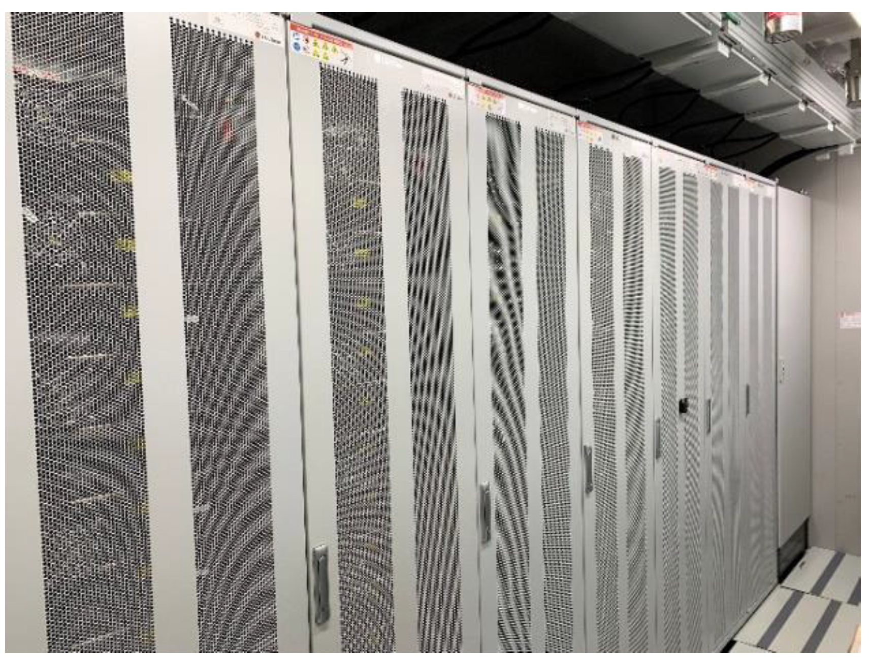
In this section, we introduce the target system and datasets used in this study. Figure 3 shows the battery modules in the ESS. We obtained the datasets from an actual ESS operated by the Korea Electrotechnology Research Institute (KERI). This system is connected to the grid of a solar power plant with a generating capacity of 250 to 640 kWh, and the LIBs are installed with a battery management system (BMS). The power conversion system (PCS) model installed in the ESS is PLABEX-H250K, which follows the SGSF-025-4 standard. The LIBs follow the KBIA-10104-02 standard, and their model is M48189P31, which was developed by LG Chem. The operational historical data of the ESS and information on the fault alarms are stored in real-time on the server. To obtain the historical data, we downloaded the dataset stored on the server based on the alarm information. The datasets are divided into PCS and SENSOR datasets. The PCS is automatically measured and stored in a system management program to monitor the status of the ESS. It is composed of 218 electrical variables observed from the PCS and batteries during ESS operation. SENSOR is a dataset measured by installing additional sensors inside the ESS room to observe the environment surrounding the battery modules. It contains 22 atmospheric variables, such as temperature and humidity. All the samples were measured and stored at various sampling frequencies (1 Hz, 1/60 Hz, 1/9000 Hz, etc.). To consider rapid changes inside the ESS room, we used samples with a sampling frequency of 1 Hz.
In this study, we used the historical data of battery overvoltage and humidity anomaly alarms generated by the system management program. A battery overvoltage alarm was declared when electrical observations are consistently measured above permissible levels. A humidity anomaly alarm was generated when the humidity values inside the ESS room were higher than a predefined threshold. This study aimed to detect abnormalities earlier than when alarms were generated by the system management program. The details of each type of anomalous datum are described in the following subsections.

3.1. Fault Alarm 1: Battery Overvoltage

Overvoltage is the most dangerous condition because it can lead to thermal runaway [42]. If overvoltage persists, the temperature and pressure inside the battery increase rapidly. To prevent overvoltage, the system management program monitors electrical variables, such as current and voltage, and the status of the battery in real-time. As mentioned above, the target system used in this study observed 18 electrical variables in real-time and accumulated them in the PCS dataset. In the system management program, an overvoltage alarm occurs when the current and voltage values of the battery are higher than predefined threshold values. From the 218 electrical variables in the PCS, we selected 8 specific variables relevant to overvoltage alarms based on the advice of the system manager. Selected variables are listed in Table 2.
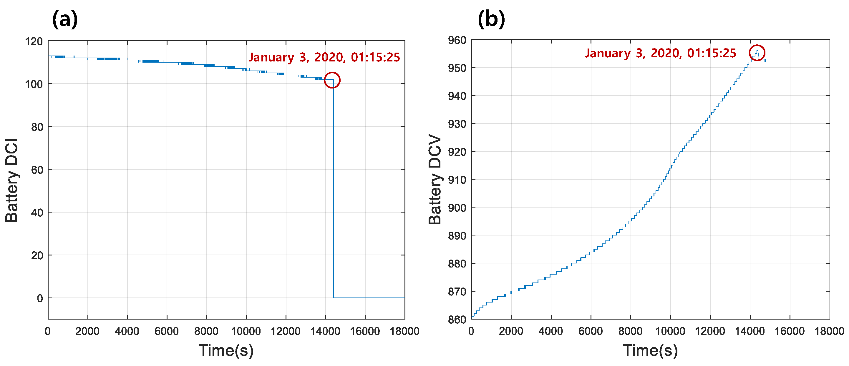
Figure 4 shows the PCS_PCS4_BAT_Cmd_DCI and PCS_PCS4_BAT_Cmd_DCV during the overvoltage alarm period. In the figures, the unit of time is second(s) and the red circles indicate the times when a battery overvoltage alarm was generated. As shown in Figure 4b, the voltage increased steadily, and an overvoltage occurred at 01:15:25 on 3 January 2020. Following the overvoltage, the system recovery mechanism rapidly reduced the current and voltage.

3.2. Fault Alarm 2: Humidity Anomaly

Because of the constant charging and discharging of batteries, the temperature inside the ESS room inevitably increases. Air conditioners operate inside the ESS room to maintain a constant ambient environment around the battery modules. Despite this, owing to unexpected factors, if the thermal runaway of a battery occurs, the temperature and pressure in the battery will increase rapidly, leading to higher humidity inside the ESS room. Therefore, to monitor the environment inside the ESS room in real-time, the system administrator installed 22 additional sensors to observe the temperature and humidity. Measured data were accumulated using the SENSOR dataset. We determined the variables used in this study with the support of the system administrator. Table 3 lists the variables selected for humidity anomaly detection. A humidity alarm was generated when the value for SENSOR_Sensor04.Temp in Table 3 exceeded 85.
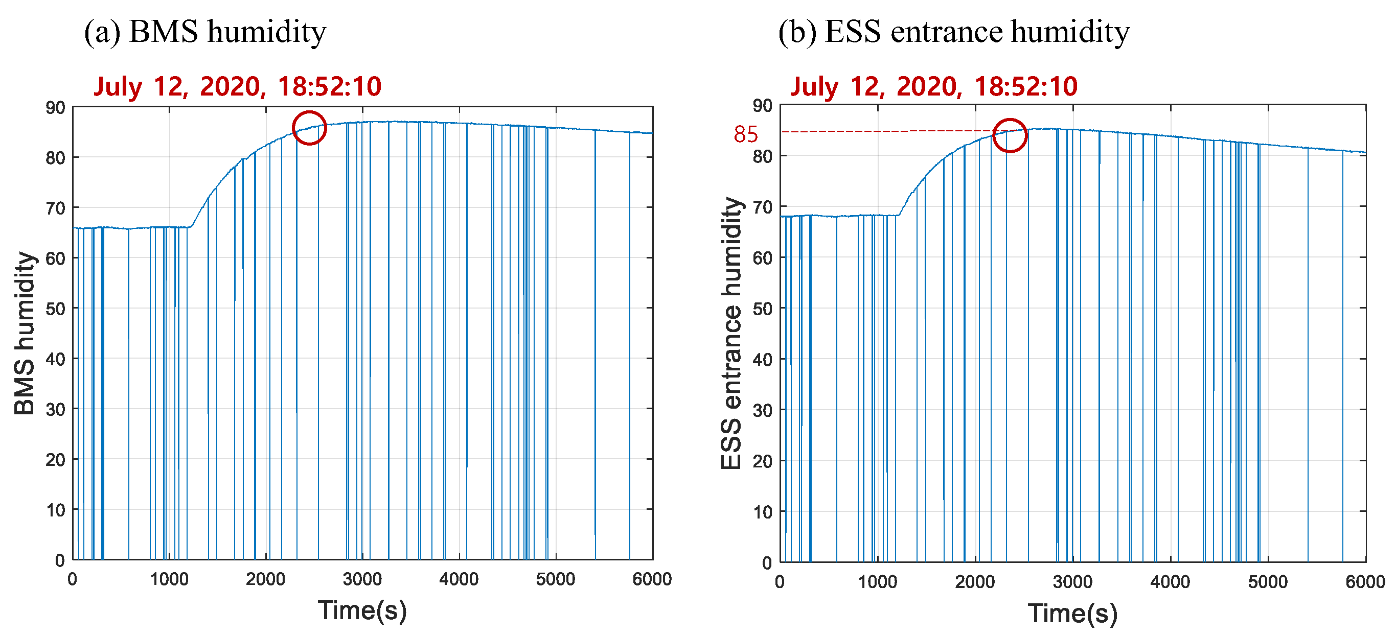
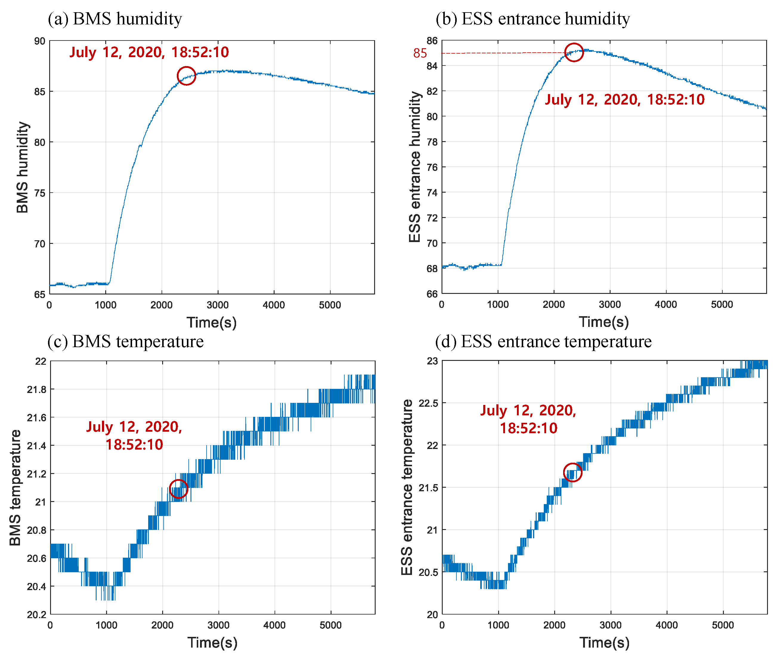
Figure 5 represents the SENSOR.Sensor03.Humi and SENSOR.Sensor04.Humi for the period of humidity anomaly. In the figures, the unit of time is second(s) and the red circles indicate when the humidity anomaly alarm occurred. As shown in Figure 5, the SENSOR had many zero values owing to communication errors between the installed sensors; therefore, these values were removed during data preprocessing. The humidity values sharply escalated at approximately t = 1200 and a humidity anomaly alarm occurred at 18:52:10 on 12 July 2020, when the value of SENSOR.Sensor04.Humi reached 85. Following the humidity anomaly, the humidity values gradually decreased owing to subsequent actions.

4. Experimental Results and Discussion

In this section, we discuss the results of the early detection of battery abnormalities using the proposed method. We conducted experiments for the early detection of battery faults through data analysis using the Statistics and Machine Learning Toolbox in MATLAB. The proposed method considers three detection indices ( I d 2 , I e 2 , and SPE statistics); however, only the results related to the best statistic, I d 2 , are given in the following subsection. To confirm the effectiveness of the proposed method, standard MD, LOF, PCA, ICA, and auto-associative kernel regression (AAKR), which are commonly used for fault detection, were selected for comparison. The detection indices of the PCA and AAKR were used as Hottelling’s T2 statistic and SPE. Both are popular statistics used for fault detection. To determine the proper ICs, we compared the results of the PCA and the proposed method. The detailed experimental results are described below. The unit of time for all figures in the following subsections is second(s).

4.1. Battery Overvoltage Alarm

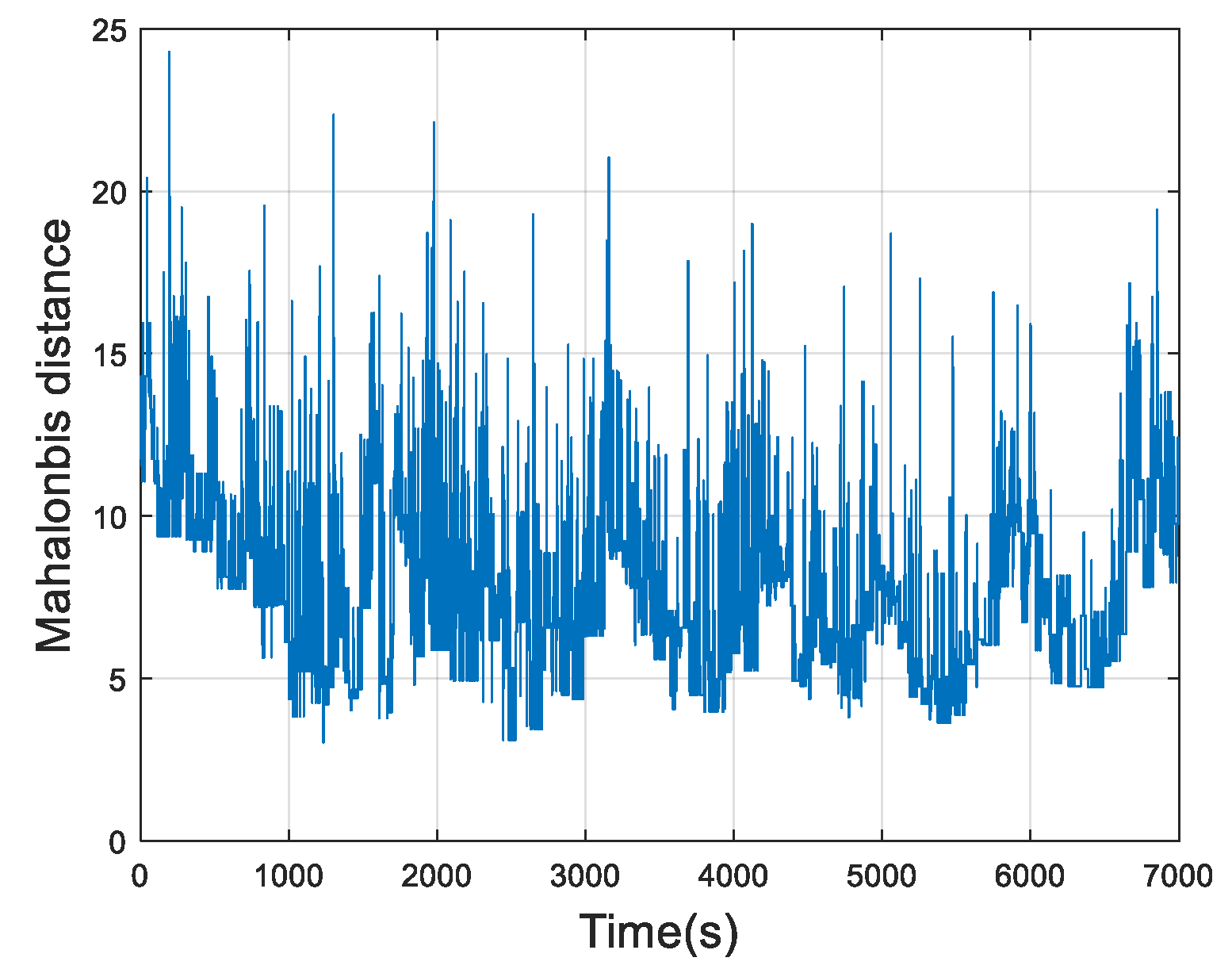
In this subsection, we introduce the results of using historical battery overvoltage data to verify the performance of the proposed method. We used 7000 samples to train the model and 5000 samples to test the performance of the proposed method. The training and test samples were normalized with zero mean and unit variance beforehand and then the MD was applied to the normalized training samples to remove outliers. Figure 6 shows the calculated MDs for the training samples. The threshold value for identifying outliers was defined as the 99th percentile of MDs through trial and error. In other words, if the MD value was more significant than the predefined threshold value, then the training vector for the MD value was considered an outlier and removed. The 99th percentile threshold was calculated to be 16.5931. Among the training samples, 71 samples were deemed to be outliers and removed, and the remaining samples were used to learn the ICA. In the online process, outliers for the test samples were removed in the same manner as above.
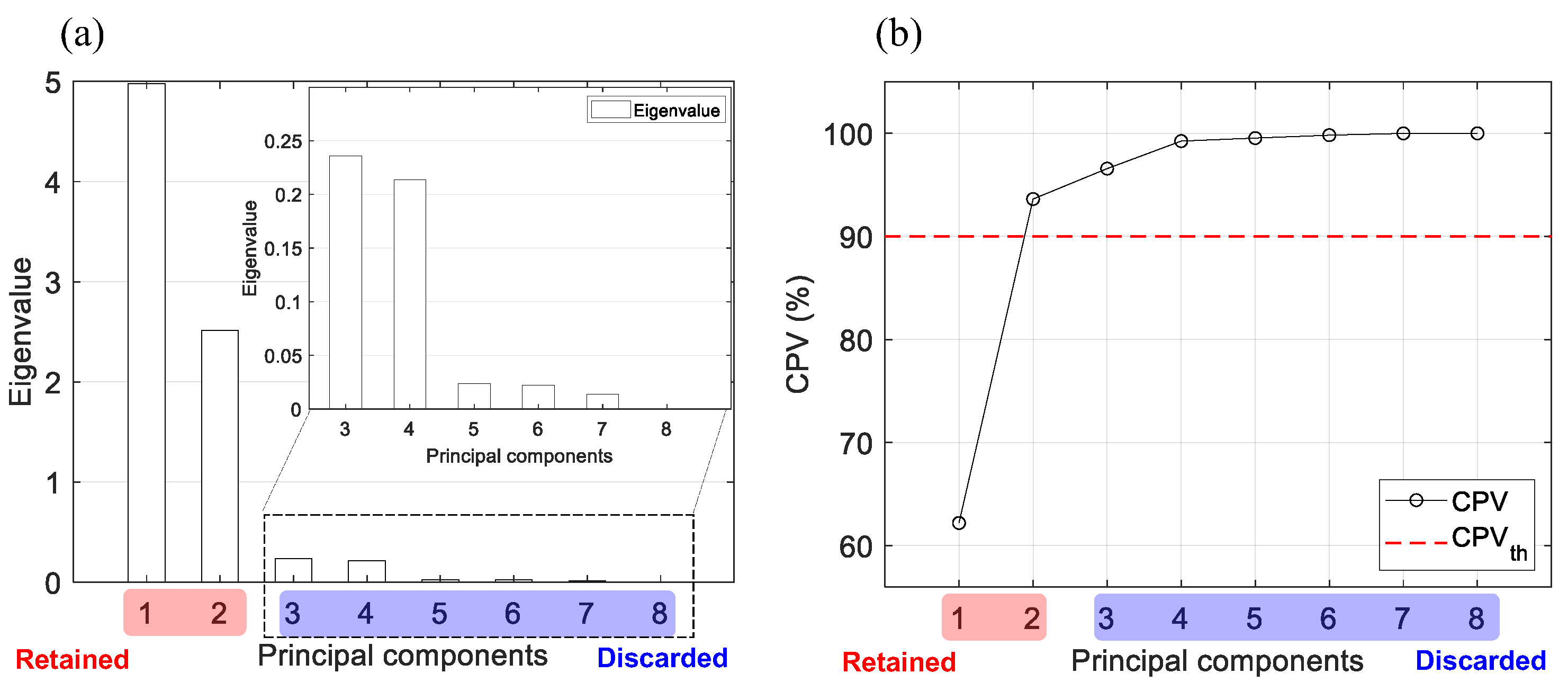
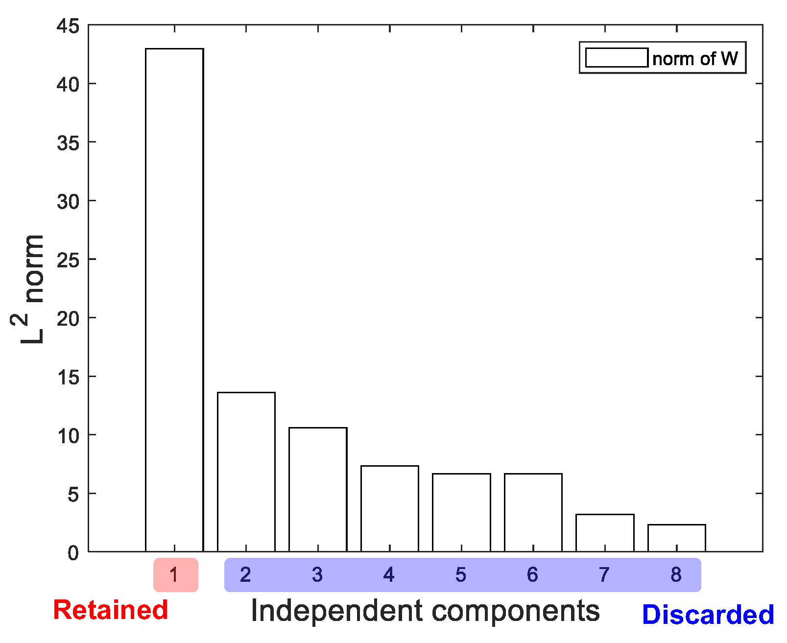
In this study, we sorted the ICs based on the Euclidean norm, a method proposed by Lee et al. [35], and determined the appropriate number of ICs by selecting the dominant parts. The ICs selected in this manner were compared with the principal components (PCs) determined using the cumulative percentage variance (CPV) in the PCA. The process for determining the number of principal components using CPV is as follows: The eigenvalues of the principal components (PCs) are calculated to obtain the variances of each PC. After sorting them in descending order, the appropriate number of PCs is determined using a predefined threshold value. This method is popular for selecting dominant PCs. Figure 7 and Figure 8 show the results of the CPV in the PCA and the Euclidean norm of the rows in W, sorted in descending order in the ICA, respectively. In Figure 7a, the variances of the first and second PCs are more dominant than those of the other PCs (enlarged figure). Therefore, we defined the threshold value as 90% for CPV. This means that only the top two PCs were retained and the others were discarded. However, in the process of selecting the dominant ICs, the norms corresponding to the first IC were extremely dominant, as shown in Figure 8; therefore, the eight dimensions can be reduced to one by selecting the first IC. Accordingly, the results of the selection of the dominant components in PCA and ICA can be different.
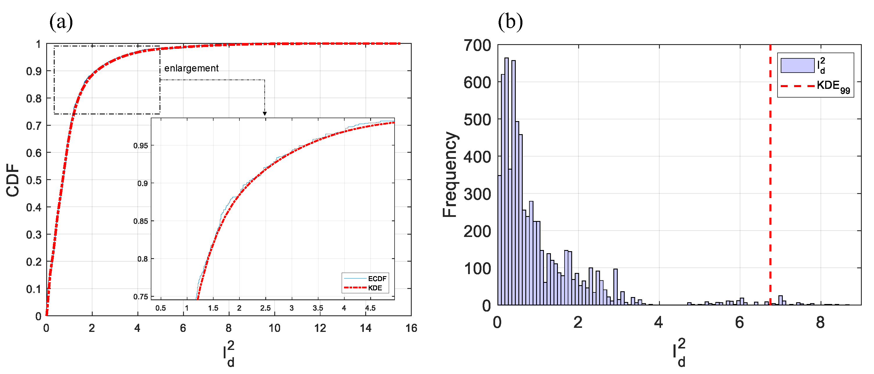
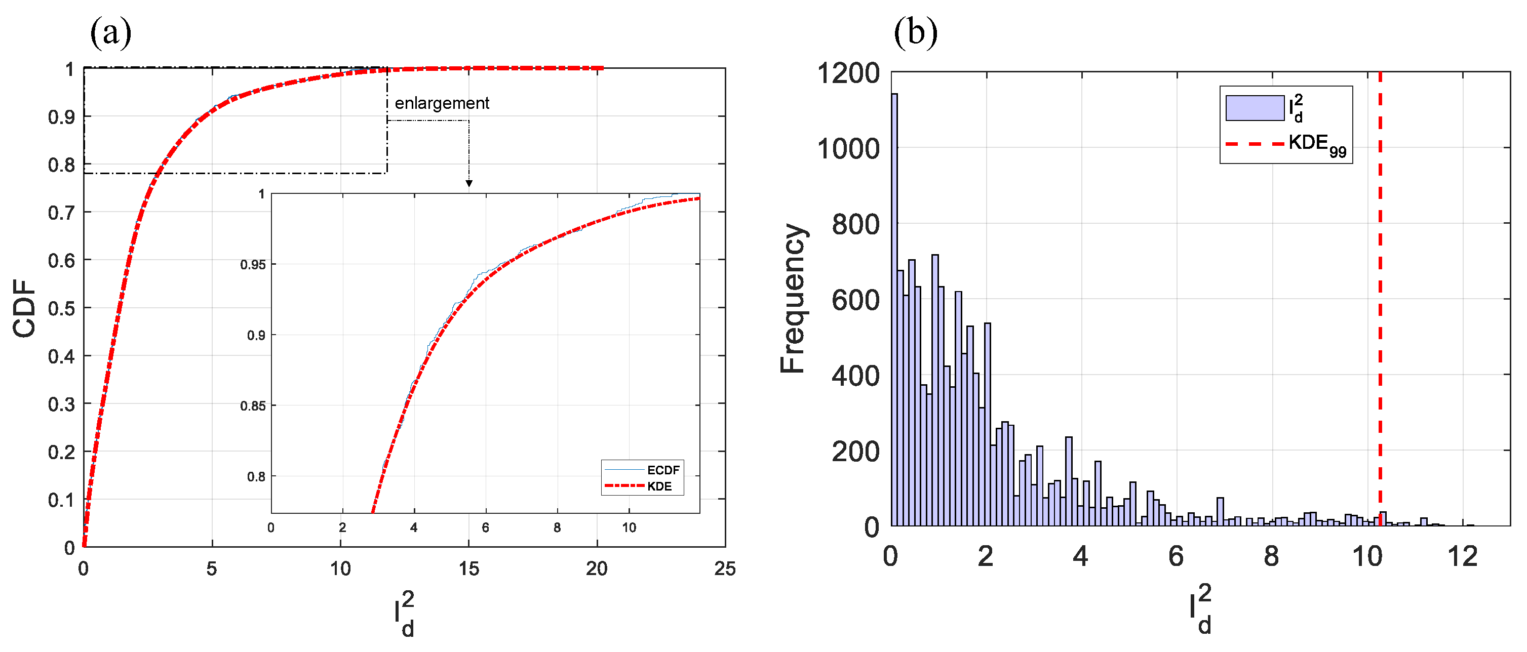
Figure 9 indicates the empirical and estimated cumulative distribution functions (CDFs) and a histogram for I d 2 calculated from the training samples of the battery overvoltage. The blue and dashed red lines represent the empirical CDF and KDE values of the detection index, respectively. In Figure 9a, an enlarged image shows that the KDE (dashed red line) was well estimated for the empirical CDF (blue line). We defined the confidence limit from the estimated CDFs with significant level α, where α was set at 0.01. We confirm the control limit with significant level α = 0.01 in Figure 9b.
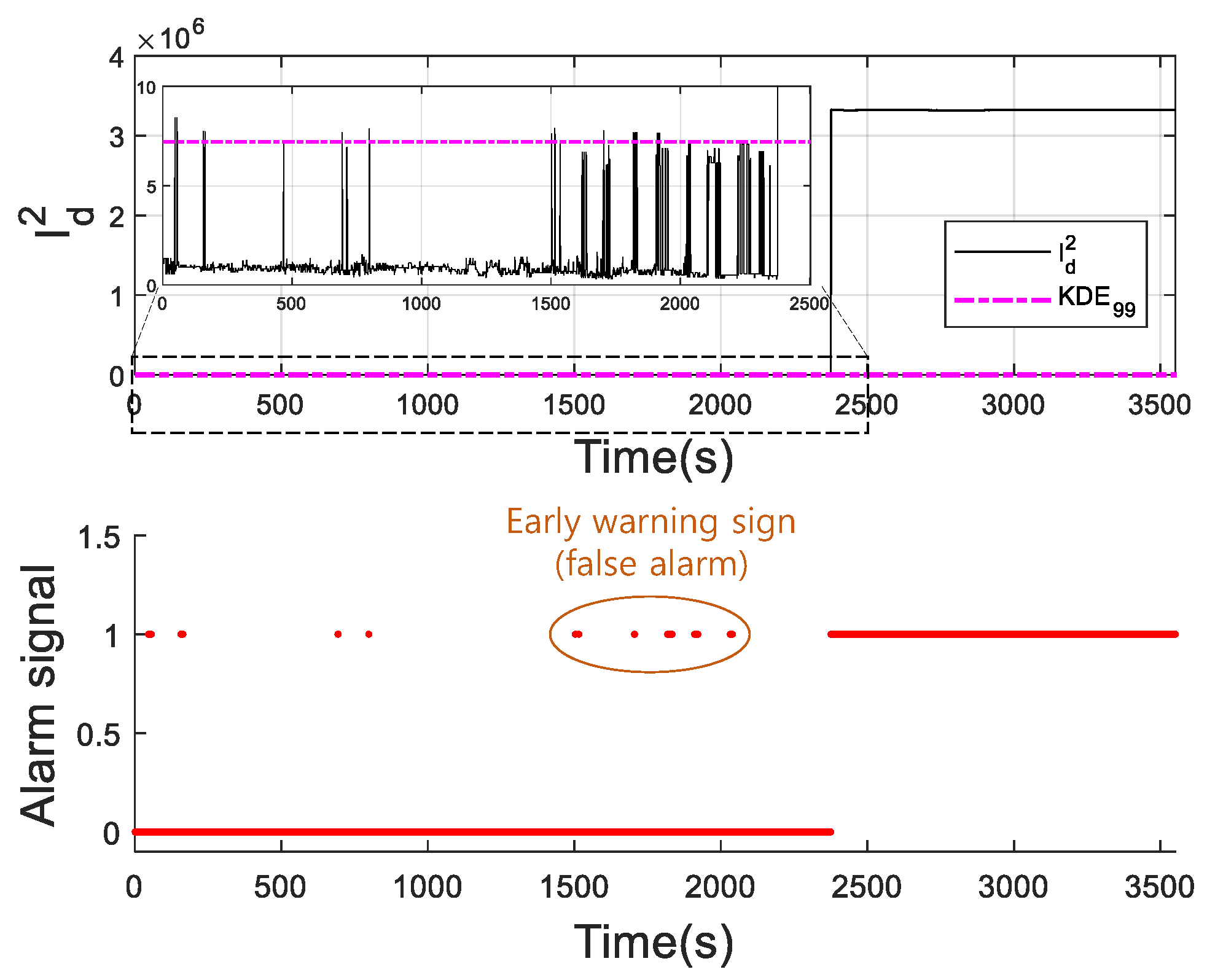
Figure 10 presents the monitoring chart and fault alarm signals of the proposed method. In Figure 10, the black line indicates the I d 2 for the test samples, the dashed purple line indicates the control limit defined by KDE, and the red dots describe the alarm signals generated when the detection index exceeded the predefined confidence limit. We recorded the time at which actual battery overvoltage occurred, and the alarm generated by the system management program was approximately t = 2400 in the monitoring chart. As depicted in Figure 10, the proposed method generates intermittent alarms even before actual overvoltage occurs. Moreover, the proposed method detects early warning signs of overvoltage by generating alarms approximately 900 s before overvoltage occurs (t = 1500 in the graph).
Figure 11 shows the monitoring charts for comparison with the proposed method. In Figure 11, the black lines indicate the detection indices for each fault detection method, the dashed purple lines indicate the confidence limits defined by the KDE, and the enlarged parts show the interval from time 0 to 2500 in each original figure. The length of the detection index of the proposed method was short because the outliers were removed using MD. The LOF (Figure 11b) and AAKR (Figure 11e) detection indices represent the trend of the battery overvoltage phenomenon, but their confidence limits were too low relative to the corresponding monitoring statistics; the confidence limit values for LOF and SPE were set to 0.3720 and 0.0026, respectively. Moreover, the control limits for MD (Figure 11a), PCA (Figure 11c), and ICA (Figure 11d) were smaller than their respective detection indices. However, in Figure 11f, the threshold value of the proposed method that was determined to be appropriate is compared with the comparison methods. Therefore, the proposed method generated proactive warning signals for battery overvoltage, as shown in Figure 10.
Table 4 lists the performance indices of the comparison and proposed methods (indicated by ‘MD + ICA’) for battery overvoltage. The performance indices for the proposed method were computed by averaging 50 independent experiments under the same conditions. This was because the experimental results differed from each other as the parameters (the matrices W, B, and Q) in ICA were randomly generated by the fastICA algorithm. In Table 4, the performance indices of the proposed method are expressed in bold, and lower indices mean better performance. The FAR for LOF and AAKR was close to 100 and the MDR was zero owing to the exceedingly low thresholds, as seen in Figure 10b,e. In the case of MD and PCA, their thresholds were determined to be low, resulting in high FARs. In contrast, the FAR for standard ICA with a properly defined confidence limit was calculated to be relatively low. However, the proposed method had the best FAR compared to others owing to its well-defined control limit by removing the outliers.

4.2. Humidity Anomaly

The experimental results of the proposed method for humidity anomaly are discussed in this subsection. As mentioned in Section 3.2, we removed the samples that measured as zero because of communication errors in the sensors. Data preprocessing was performed on the SENSOR dataset to remove these values because not banishing them may have led to biased training results for the model. Figure 12 shows the test data of the selected variables from SENSOR with zero-value samples removed. In the figures, the red circles indicate the time required for the humidity anomaly alarm. We used 14,000 and 2500 samples from SENSOR to learn and test the models, respectively.
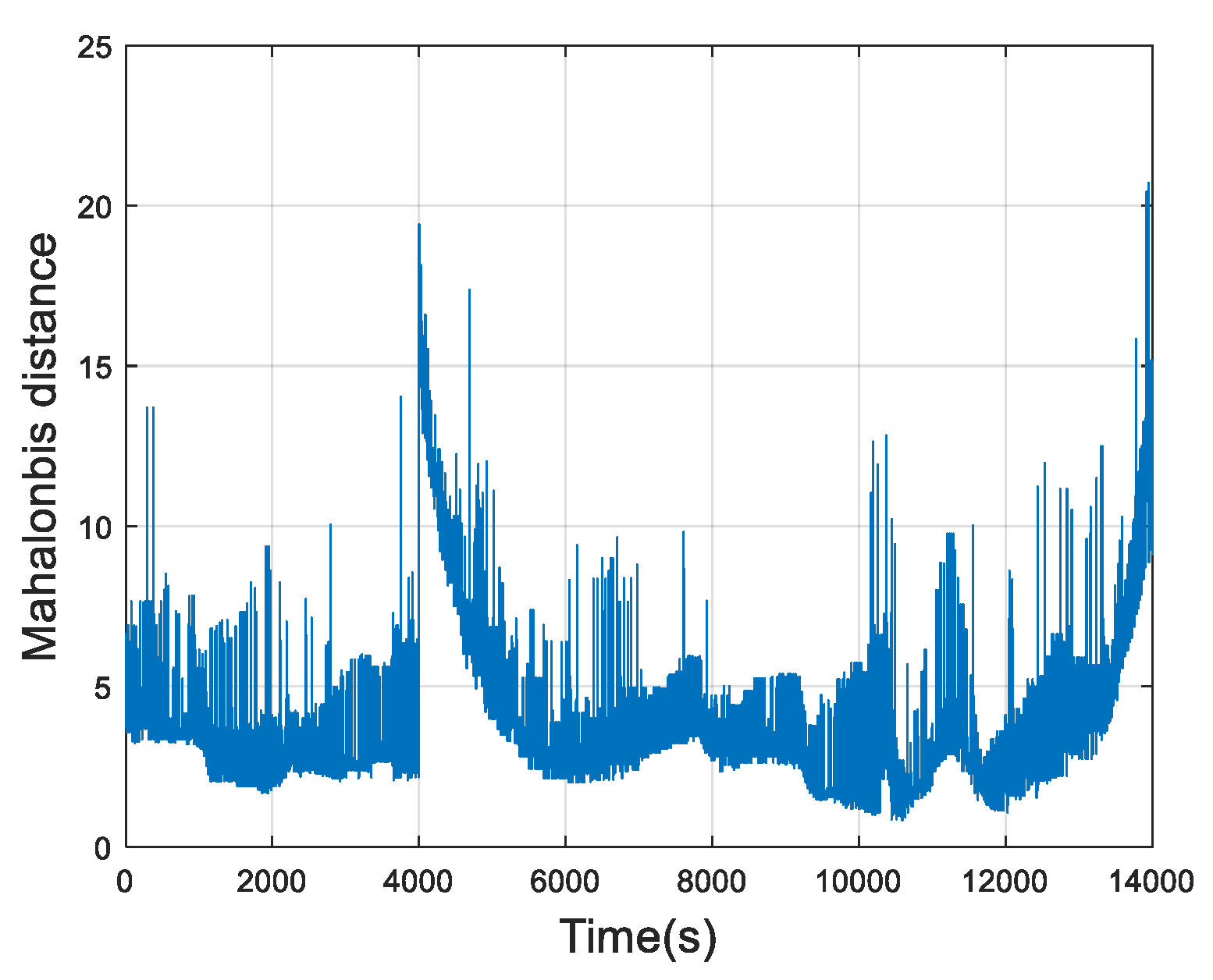
Each variable was normalized before applying MD. After normalization, MD was applied to the normalized training sample, as shown in Figure 13. Outliers were removed based on the 99th percentile of the MD for the training samples. In this case, the threshold value was calculated to be 13.531; 138 samples were considered outliers, and the remaining 13,862 samples were used to train the ICA.
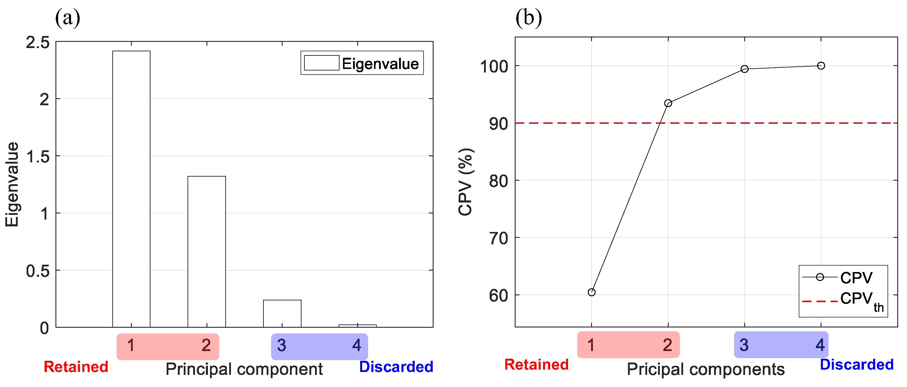
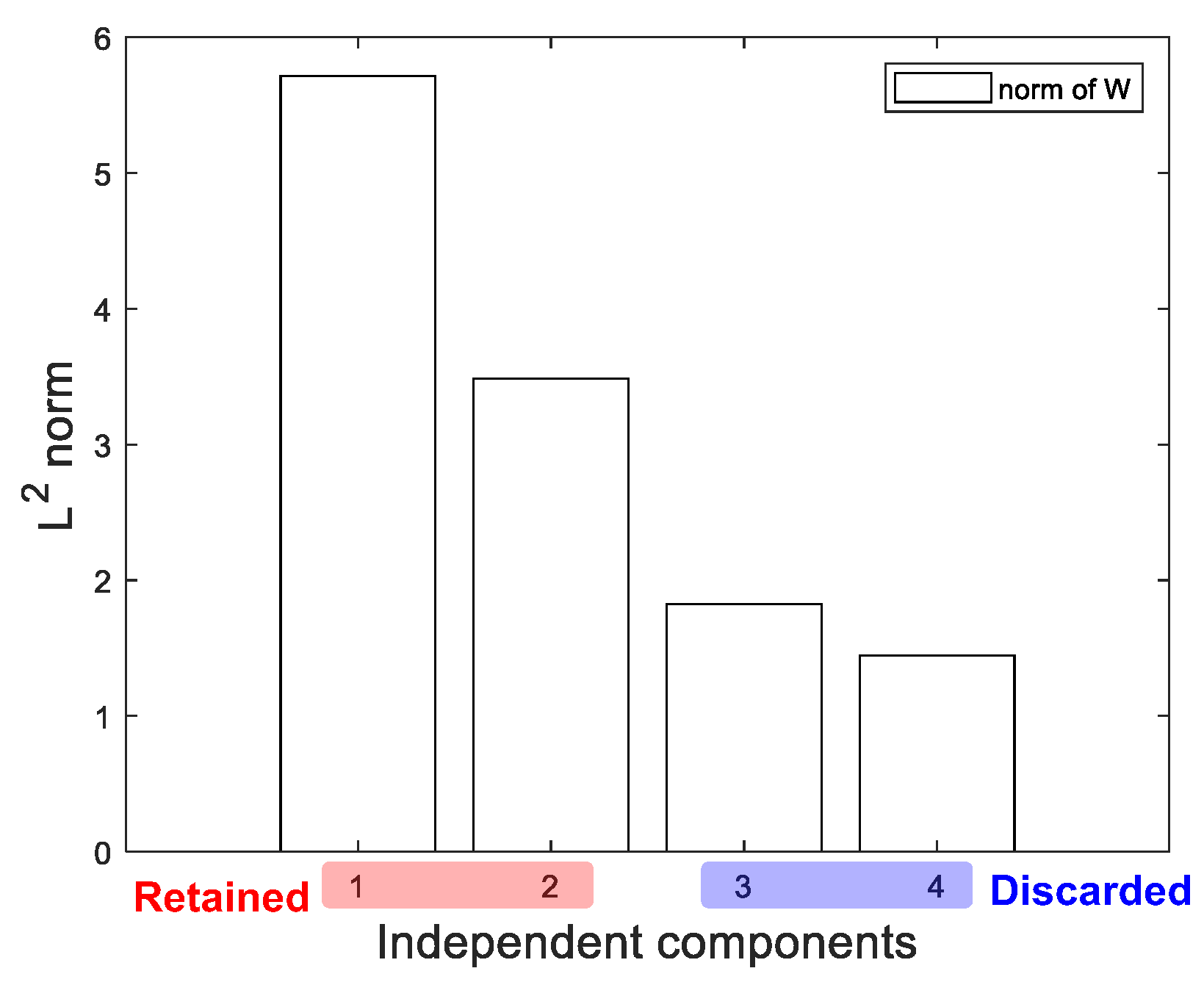
Figure 14 illustrates the experimental results for determining the dominant PCs using CPV in PCA. In Figure 14a, we confirm that the eigenvalues of the top two PCs were dominant compared to those of the others. Thus, to select the top two PCs, we defined the threshold value as 90 in the CPV, as depicted in Figure 14b. Figure 15 shows the L2 norms of the rows in W, sorted in descending order. In contrast to Figure 14a, the Euclidean norms of the third and fourth ICs were relatively high. Thus, to consider ICs, we conducted iterative experiments by adjusting the dimensions. After repeated experiments, the best performance was achieved when only the top two ICs were selected, and the four dimensions were reduced to two.
Figure 16 shows the empirical and estimated cumulative distribution functions (CDFs) and a histogram of I d 2 calculated from the training samples of the humidity anomaly case. The enlarged image in Figure 16a indicates that the KDE was similar to the empirical CDF. The same as in the battery overvoltage case, we defined the confidence limits with significant level α = 0.01 from estimated CDFs. The threshold values are shown in Figure 16b.
Figure 17 shows the monitoring chart and fault alarm signals of the proposed method. In Figure 17, the black line, dotted purple line, and red dots indicate the I d 2 calculated from the test sample, control limit determined by the KDE, and fault alarm signals generated by exceeding the detection index of the control limit, respectively. The actual humidity anomaly alarm from the program management system occurred at time t = 2270, whereas the detection index of the proposed method continuously violated the confidence limit at approximately t = 1100. In addition, the proposed method continuously generated early warning signs (false alarms) for 420 s, starting at approximately t = 680. This means that the proposed method conducts early detection of humidity anomalies and can provide additional time for field managers to solve this problem.
Considering the monitoring charts of the comparison and proposed methods in Figure 18, the enlarged parts in Figure 18 correspond to the period from 0 s to 1200 s for each monitoring chart. The thresholds for LOF (Figure 18b) and AAKR (Figure 18e) were defined as extremely low, as in the case of battery overvoltage, whereas the control limits for MD (Figure 18a), PCA (Figure 18c), and ICA (Figure 18d) were determined to be relatively high. In contrast, the confidence limit was violated when the detection index increased rapidly because the threshold of the proposed method (Figure 18f) was set appropriately. In other words, the proposed method can accurately capture the possibility of increasing humidity relative to the comparison methods. In other words, the proposed method captured the possibility of increasing the humidity more accurately than the comparison method.
Table 5 lists each performance index computed from the comparison and proposed methods for humidity anomaly. As with battery overvoltage, the thresholds for LOF and AAKR were set too low, which led to a FAR close to 100 and an MDR of zero. On the other hand, the performance indices of the comparison methods, except LOF and AAKR, were acceptable; PCA and ICA had slightly higher thresholds, resulting in an extremely low FAR but a relatively high MDF. The control limit of the MD was determined moderately compared to PCA and ICA; therefore, its MDR was calculated to be low. In the case of the proposed method, the MDR was significantly low compared to other comparison methods, but its FAR was slightly high owing to some false alarms. The false alarms were acceptable because they provided an early warning of a rapid increase in humidity.

4.3. Discussion

This subsection summarizes the advantages of this study. Its main strength is the early detection of two types of battery anomalies in a real-world ESS using MD and ICA. The anomalous data used in this study were battery overvoltage and humidity anomalies, which are typical antecedents to the thermal runaway of LIBs. The thermal runaway of LIBs occurs when the pressure inside the battery increases and the temperature grows rapidly and uncontrollably. This can lead to fire accidents in the overall system; therefore, monitoring technology for LIBs is required to proactively prevent thermal runaway. In Table 4 and Table 5, the superiority of the proposed method over conventional fault detection models by removing outliers is demonstrated. Moreover, Figure 10 and Figure 17 show that the method detected anomalies earlier than when the alarms were generated by the system management program: 15 min earlier for battery overvoltage and 26 min earlier for humidity anomaly. This means that we can obtain additional time for system managers to solve problems.
A common antecedent of battery overvoltage is increasing voltage due to continuous battery charging. In the case of humidity anomaly, the humidity inside the ESS room gradually increases in the form of drift before the humidity anomaly alarm is triggered. The proposed method was able to detect anomalies by learning the real-world data with these properties. Therefore, the proposed method will work effectively in other battery systems as well.

5. Conclusions

Batteries are used to store and supply power in various industries. In particular, power grids such as ESSs are essential for efficient energy management. In recent years, LIBs have been used in industrial fields owing to their high energy density and low memory effect; however, the frequency of battery fires due to thermal runaway has increased. A fire in a system such as an electric vehicle or ESS can cause significant damage; therefore, monitoring methods are needed to detect battery anomalies proactively. In this study, we used the historical data of battery overvoltage and humidity anomalies related to fire accidents from LIBs operating in a real-world ESS. The two types of anomalies were indicated by alarms generated by the system management program. The system management program declared alarms based on simple thresholds. For example, the humidity anomaly alarm automatically occurred when the real-time observation of ‘SENSOR.Sensor04.Humi’ reached 85. If a fire occurs in an ESS, the humidity inside the ESS room will increase very quickly, indicating that threshold-based alarm generation methods can be risky.
We used MD to remove outliers from an industrial dataset and conducted the early detection of two types of faults using ICA. The ICA used in the proposed method could efficiently learn useful information by removing redundant parts. In other words, determining how much to reduce the dimensions is a crucial issue in ICA. To address this problem, we conducted experiments comparing it to PCA, a popular dimensionality reduction method. In addition, the comparison methods in this study had poor performance due to improperly determined confidence limits. However, the confidence limits of the proposed method were well defined because they were computed based on normal samples from which outliers had been excluded by MD; this allowed for the generation of fault alarms faster than the system management program. The experimental results show that the proposed method can successfully detect hazards earlier than the alarms generated by the ESS integrated monitoring system by 15 min and 26 min for battery overvoltage and humidity abnormality, respectively. In addition, the proposed method demonstrated superior performance compared to conventional fault detection methods.
In future research, we will consider the following topics. The first topic is the fault identification of historical battery fault data. Fault identification is a method for identifying the failure variables that contribute to the failure of a target system. This study achieved the early detection of two types of battery anomalies; however, if we can find the fault variables among the process variables, this could enable us to analyze and respond to failures efficiently. The second topic is the study of effective feature extraction methods to improve fault detection performance. We did not conduct in-depth research on feature extraction in this study. The presence or absence of effective feature extraction can significantly alter the performance of machine learning and statistical methods. Therefore, we will perform a study on feature extraction to improve fault detection performance. The last topic is the practical validation of the proposed method. In this study, the proposed method was validated by real-world industrial data using MATLAB. The dataset consisted of two types of historical battery fault data obtained from an actual operational energy storage system. The performance of the proposed method was demonstrated through a comparison with existing fault detection models, such as distance-based methods (LOF, MD) and multivariate statistical methods (PCA, standard ICA, AAKR). In the future, we will install this algorithm into the target system (real-world ESS) and proceed with practical validation.

Author Contributions

Conceptualization, S.J. and M.K.; methodology, S.J.; software, B.K.; validation, S.J. and M.K.; formal analysis, E.K.; investigation, M.K.; resources, K.-H.C. and H.-A.P.; data curation, K.-H.C. and H.-A.P.; writing—original draft preparation, S.J. and M.K.; writing—review and editing, J.K., B.K., E.K. and S.K.; visualization, S.J.; supervision, S.K. All authors have read and agreed to the published version of the manuscript.

Funding

This work was supported by the National Research Foundation of Korea (NRF), grant funded by the Korea government (MSIT) (No. 2021R1A2C2009667).

Data Availability Statement

Data are contained within the article.

Acknowledgments

This work was supported by the National Research Foundation Korea (NRF), grant funded by the Korean government (MSIT) (grant No. 2021R1A2C2009667), and the Technological Innovation R&D Program (S3238625), funded by the Ministry of SMEs and Startups (MSS, Korea).

Conflicts of Interest

The authors declare no conflicts of interest.

References

  1. Nasiri, F.; Ooka, R.; Haghighat, F.; Shirzadi, N.; Dotoli, M.; Carli, R.; Scarabaggio, P.; Behzadi, A.; Rahnama, S.; Afshari, A.; et al. Data analytics and information technologies for smart energy storage systems: A state-of-the-art review. Sustain. Cities Soc. 2022, 84, 104004. [Google Scholar] [CrossRef]
  2. Rahman, F.; Rehman, S.; Abdul-Majeed, M.A. Overview of energy storage systems for storing electricity from renewable energy sources in Saudi Arabia. Renew. Sustain. Energy Rev. 2012, 16, 274–283. [Google Scholar] [CrossRef]
  3. Evans, A.; Strezov, V.; Evans, T.J. Assessment of utility energy storage options for increased renewable energy penetration. Renew. Sustain. Energy Rev. 2012, 16, 4141–4147. [Google Scholar] [CrossRef]
  4. Chavan, S.; Rudrapati, R.; Manickam, S. A comprehensive review on current advances of thermal energy storage and its applications. Alex. Eng. J. 2022, 61, 5455–5463. [Google Scholar] [CrossRef]
  5. Selvakumar, R.D.; Wu, J.; Ding, Y.; Alkaabi, A.K. Melting behavior of an organic phase change material in a square thermal energy storage capsule with an array of wire electrodes. Appl. Therm. Eng. 2023, 228, 120492. [Google Scholar] [CrossRef]
  6. Tran, M.K.; Mevawalla, A.; Aziz, A.; Panchal, S.; Xie, Y.; Fowler, M. A review of lithium-ion battery thermal runaway modeling and diagnosis approaches. Processes 2022, 10, 1192. [Google Scholar] [CrossRef]
  7. Wang, Q.; Mao, B.; Stoliarov, S.I.; Sun, J. A review of lithium ion battery failure mechanisms and fire prevention strategies. Prog. Energy Combust. Sci. 2019, 73, 95–131. [Google Scholar] [CrossRef]
  8. Qi, C.; Zhu, Y.; Gao, F.; Yang, K.; Jiao, Q. Mathematical model for thermal behavior of lithium ion battery pack under overcharge. Int. J. Heat Mass Transf. 2018, 124, 552–563. [Google Scholar] [CrossRef]
  9. Lystianingrum, V.; Hredzak, B.; Agelidis, V.G. Multiple model estimator based detection of abnormal cell overheating in a Li-ion battery string with minimum number of temperature sensors. J. Power Sources 2015, 273, 1171–1181. [Google Scholar] [CrossRef]
  10. Pan, Y.; Feng, X.; Zhang, M.; Han, X.; Lu, L.; Ouyang, M. Internal short circuit detection for lithium-ion battery pack with parallel-series hybrid connections. J. Clean. Prod. 2020, 255, 120277. [Google Scholar] [CrossRef]
  11. Dong, G.; Lin, M. Model-based thermal anomaly detection for lithium-ion batteries using multiple-model residual generation. J. Energy Storage 2021, 40, 102740. [Google Scholar] [CrossRef]
  12. Feng, X.; Pan, Y.; He, X.; Wang, L.; Ouyang, M. Detecting the internal short circuit in large-format lithium-ion battery using model-based fault-diagnosis algorithm. J. Energy Storage 2018, 18, 26–39. [Google Scholar] [CrossRef]
  13. Tran, M.K.; Panchal, S.; Chauhan, V.; Brahmbhatt, N.; Mevawalla, A.; Fraser, R.; Fowler, M. Python-based scikit-learn machine learning models for thermal and electrical performance prediction of high-capacity lithium-ion battery. Int. J. Energy Res. 2022, 46, 786–794. [Google Scholar] [CrossRef]
  14. Haider, S.N.; Zhao, Q.; Li, X. Data driven battery anomaly detection based on shape based clustering for the data centers class. J. Energy Storage 2020, 29, 101479. [Google Scholar] [CrossRef]
  15. Yao, L.; Xiao, Y.; Gong, X.; Hou, J.; Chen, X. A novel intelligent method for fault diagnosis of electric vehicle battery system based on wavelet neural network. J. Power Sources 2020, 453, 227870. [Google Scholar] [CrossRef]
  16. Tran, M.K.; Fowler, M. A review of lithium-ion battery fault diagnostic algorithms: Current progress and future challenges. Algorithms 2020, 13, 62. [Google Scholar] [CrossRef]
  17. Ma, M.; Li, X.; Gao, W.; Sun, J.; Wang, Q.; Mi, C. Multi-fault diagnosis for series-connected lithium-ion battery pack with reconstruction-based contribution based on parallel PCA-KPCA. Appl. Energy 2022, 324, 119678. [Google Scholar] [CrossRef]
  18. Yao, L.; Wang, Z.; Ma, J. Fault detection of the connection of lithium-ion power batteries based on entropy for electric vehicles. J. Power Sources 2015, 293, 548–561. [Google Scholar] [CrossRef]
  19. Xiong, J.; Banvait, H.; Li, L.; Chen, Y.; Xie, J.; Liu, Y.; Wu, M.; Chen, J. Failure detection for over-discharged Li-ion batteries. In Proceedings of the 2012 IEEE International Electric Vehicle Conference, Greenville, SC, USA, 4–8 March 2012; pp. 1–5. [Google Scholar]
  20. Kang, Y.; Duan, B.; Zhou, Z.; Shang, Y.; Zhang, C. A multi-fault diagnostic method based on an interleaved voltage measurement topology for series connected battery packs. J. Power Sources 2019, 417, 132–144. [Google Scholar] [CrossRef]
  21. Ma, M.; Wang, Y.; Duan, Q.; Wu, T.; Sun, J.; Wang, Q. Fault detection of the connection of lithium-ion power batteries in series for electric vehicles based on statistical analysis. Energy 2018, 164, 745–756. [Google Scholar] [CrossRef]
  22. Gajjar, S.; Palazoglu, A. A data-driven multidimensional visualization technique for process fault detection and diagnosis. Chemom. Intell. Lab. Syst. 2016, 154, 122–136. [Google Scholar] [CrossRef]
  23. Sun, X.; Marquez, H.J.; Chen, T.; Riaz, M. An improved PCA method with application to boiler leak detection. ISA Trans. 2005, 44, 379–397. [Google Scholar] [CrossRef] [PubMed]
  24. Dong, G.; Wei, J.; Zhang, C.; Chen, Z. Online state of charge estimation and open circuit voltage hysteresis modeling of LiFePO4 battery using invariant imbedding method. Appl. Energy 2016, 162, 163–171. [Google Scholar] [CrossRef]
  25. Kim, S.J.; Lee, S.Y.; Cho, K.S. Design of high-performance unified circuit for linear and non-linear SVM classifications. JSTS J. Semicond. Technol. Sci. 2012, 12, 162–167. [Google Scholar] [CrossRef]
  26. Lucu, M.; Martinez-Laserna, E.; Gandiaga, I.; Liu, K.; Camblong, H.; Widanage, W.D.; Marco, J. Data-driven nonparametric Li-ion battery ageing model aiming at learning from real operation data-Part B: Cycling operation. J. Energy Storage 2020, 30, 101410. [Google Scholar] [CrossRef]
  27. Hong, J.; Wang, Z.; Yao, Y. Fault prognosis of battery system based on accurate voltage abnormity prognosis using long short-term memory neural networks. Appl. Energy 2019, 251, 113381. [Google Scholar] [CrossRef]
  28. Yao, Q.; Lu, D.D.C.; Lei, G. A simple internal resistance estimation method based on open circuit voltage test under different temperature conditions. In Proceedings of the 2018 IEEE International Power Electronics and Application Conference and Exposition (PEAC), Shenzhen, China, 4–7 November 2018; pp. 1–4. [Google Scholar]
  29. Badmos, O.; Kopp, A.; Bernthaler, T.; Schneider, G. Image-based defect detection in lithium-ion battery electrode using convolutional neural networks. J. Intell. Manuf. 2020, 31, 885–897. [Google Scholar] [CrossRef]
  30. Qiu, Y.; Dong, T.; Lin, D.; Zhao, B.; Cao, W.; Jiang, F. Fault diagnosis for lithium-ion battery energy storage systems based on local outlier factor. J. Energy Storage 2022, 55, 105470. [Google Scholar] [CrossRef]
  31. Kumar, S.; Chow, T.W.; Pecht, M. Approach to fault identification for electronic products using Mahalanobis distance. IEEE Trans. Instrum. Meas. 2009, 59, 2055–2064. [Google Scholar] [CrossRef]
  32. Lee, J.M.; Yoo, C.; Lee, I.B. Statistical monitoring of dynamic processes based on dynamic independent component analysis. Chem. Eng. Sci. 2004, 59, 2995–3006. [Google Scholar] [CrossRef]
  33. Martin, E.; Morris, A. Non-parametric confidence bounds for process performance monitoring charts. J. Process Control 1996, 6, 349–358. [Google Scholar] [CrossRef]
  34. Hyvarinen, A. Fast and robust fixed-point algorithms for independent component analysis. IEEE Trans. Neural Netw. 1999, 10, 626–634. [Google Scholar] [CrossRef] [PubMed]
  35. Lee, J.M.; Yoo, C.; Lee, I.B. Statistical process monitoring with independent component analysis. J. Process Control 2004, 14, 467–485. [Google Scholar] [CrossRef]
  36. Hyvärinen, A.; Oja, E. Independent component analysis: Algorithms and applications. Neural Netw. 2000, 13, 411–430. [Google Scholar] [CrossRef]
  37. Cheung, Y.M.; Xu, L. An empirical method to select dominant independent components in ICA for time series analysis. In Proceedings of the IJCNN’99. International Joint Conference on Neural Networks. Proceedings (Cat. No. 99CH36339), Washington, DC, USA, 10–16 July 1999; Volume 6, pp. 3883–3887. [Google Scholar]
  38. Hyvarinen, A. Survey on independent component analysis. Neural Comput. Surv. 1999, 2, 94–128. [Google Scholar]
  39. Yu, J.; Yoo, J.; Jang, J.; Park, J.H.; Kim, S. A novel hybrid of auto-associative kernel regression and dynamic independent component analysis for fault detection in nonlinear multimode processes. J. Process Control 2018, 68, 129–144. [Google Scholar] [CrossRef]
  40. Silverman, B.W. Density Estimation for Statistics and Data Analysis; Routledge: Milton Park, UK, 2018. [Google Scholar]
  41. Wand, M.P.; Jones, M.C. Kernel Smoothing; CRC Press: Boca Raton, FL, USA, 1994. [Google Scholar]
  42. Barsukov, Y. Secondary Batteries–Lithium Rechargeable Systems|Hazards and Protection Circuits. In Encyclopedia of Electrochemical Power Sources; Elsevier: Amsterdam, The Netherlands; Academic Press: Cambridge, MA, USA, 2009; Volume 5, pp. 177–183. [Google Scholar]
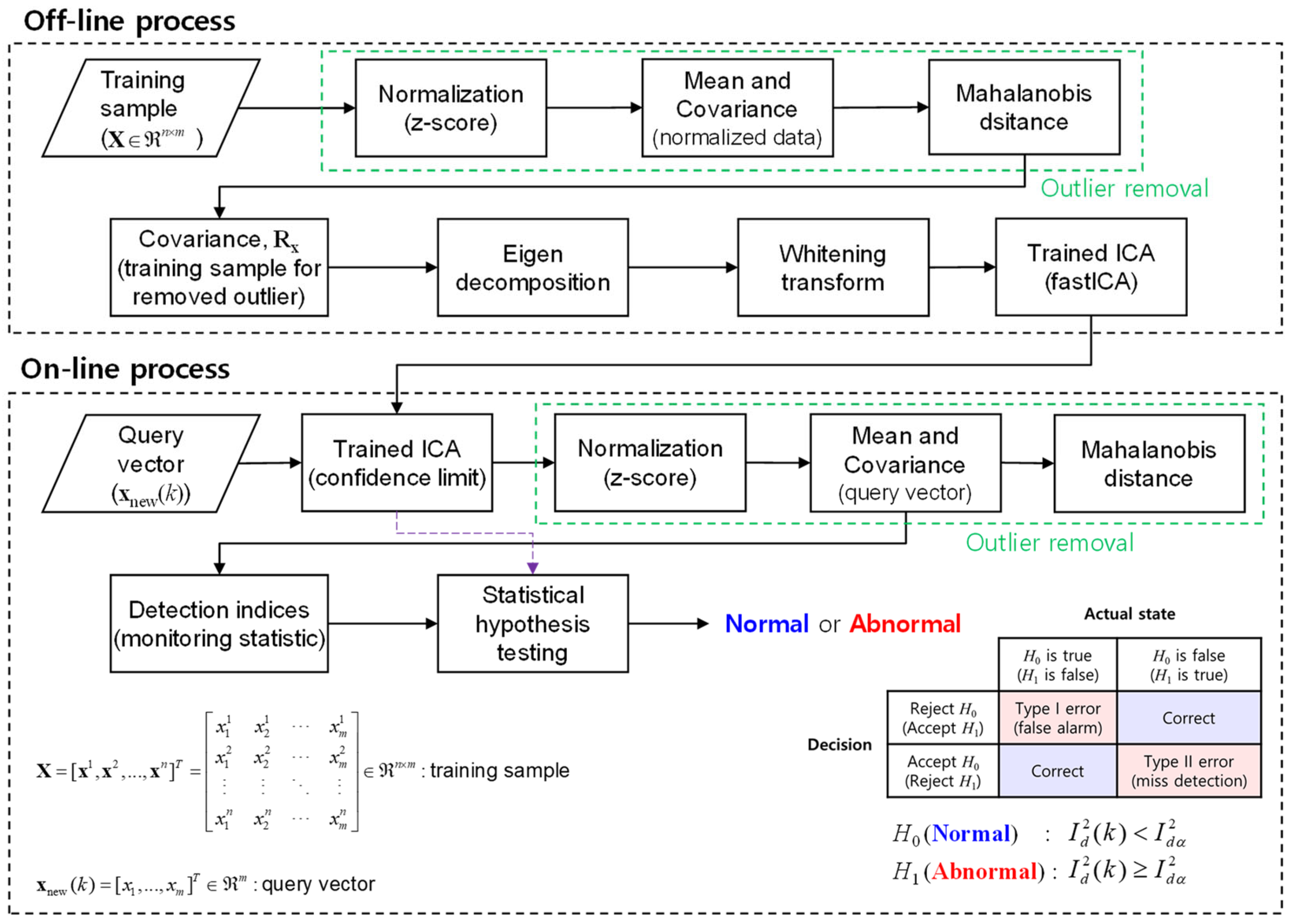
Figure 1. Framework of the proposed method for fault detection.
Energies 17 00535 g001
Figure 2. Flowchart of the proposed method for fault detection.
Energies 17 00535 g002
Figure 3. Battery modules in the ESS room.
Energies 17 00535 g003
Figure 4. Examples of battery current and voltage variables for the period of overvoltage: (a) PCS_PCS4_BAT_Cmd_DCI; (b) PCS_PCS4_BAT_Cmd_DCV.
Energies 17 00535 g004
Figure 5. Examples of humidity variables for the period of humidity anomaly: (a) SENSOR.Sensor03.Humi; (b) SENSOR.Sensor04.Humi.
Energies 17 00535 g005
Figure 6. MD for the normalized training samples (overvoltage).
Energies 17 00535 g006
Figure 7. The results of selecting the dominant PCs using CPV (overvoltage): (a) eigenvalues; (b) CPV and threshold values.
Energies 17 00535 g007
Figure 8. The results of selecting the dominant ICs using L2 norm (overvoltage).
Energies 17 00535 g008
Figure 9. Empirical and estimated CDFs and histogram plot of I d 2 calculated from the training data (overvoltage): (a) empirical and estimated CDF via KDE; (b) histogram and confidence limit.
Energies 17 00535 g009
Figure 10. Monitoring chart and fault alarm signals of the proposed method (overvoltage).
Energies 17 00535 g010
Figure 11. Monitoring charts of the proposed and comparison method (overvoltage): (a) MD; (b) LOF; (c) PCA; (d) ICA; (e) AAKR; (f) MD + ICA (proposed method).
Energies 17 00535 g011
Figure 12. Test samples for selected variables with zero-value samples removed (humidity anomaly).
Energies 17 00535 g012
Figure 13. MD for normalized training samples (humidity anomaly).
Energies 17 00535 g013
Figure 14. The results of selecting the dominant PCs using CPV (humidity anomaly): (a) eigenvalues; (b) CPV and threshold values.
Energies 17 00535 g014
Figure 15. The results of selecting the dominant ICs using L2 norm (humidity anomaly).
Energies 17 00535 g015
Figure 16. Empirical and estimated CDFs and histogram plot of I d 2 calculated from the training data (humidity anomaly): (a) empirical and estimated CDF via KDE; (b) histogram and confidence limit.
Energies 17 00535 g016
Figure 17. Monitoring chart and fault alarm signals of the proposed method (humidity anomaly).
Energies 17 00535 g017
Figure 18. Monitoring charts of the proposed and comparison methods (humidity anomaly): (a) MD; (b) LOF; (c) PCA; (d) standard ICA; (e) AAKR; (f) MD + ICA (proposed method).
Energies 17 00535 g018
Table 1. Performance indices based on statistical hypothesis testing.
Decision
Reject H0
(Accept H1)
Accept H0
(Reject H1)
TruthH0 is true
(H1 is false)
FAR
(Type I error)
Correct decision
H0 is false
(H1 is true)
Correct decisionMDR
(Type II error)
Table 2. Selected variables for overvoltage detection.
No.VariablesDescriptionUnit
1PCS_PCS4_BAT_Cmd_DCIBattery DC currentA
2PCS_PCS4_BAT_Cmd_DCVBattery DC voltageV
3PCS_PCS4_BAT_Cmd_SOCBattery state of charge%
4PCS_PCS4_DCIPCS DC currentA
5PCS_PCS4_DCVPCS DC voltageV
6PCS_PCS4_GridIaPhase current RA
7PCS_PCS4_GridIbPhase current SA
8PCS_PCS4_GridIcPhase current TA
Table 3. Selected variables for humidity anomaly detection.
No.VariablesDescriptionUnit
1SENSOR.Sensor03.HumiBMS humidity in ESS room%
2SENSOR.Sensor03.TempBMS temperature in ESS room°C
3SENSOR.Sensor04.HumiESS room entrance humidity%
4SENSOR.Sensor04.TempESS room entrance temperature°C
Table 4. Performance indices of the proposed and comparison methods (overvoltage).
Fault Type IndicesMDLOFPCAICAAAKRMD + ICA
MDLOFT2 I d 2 SPE I d 2
Battery overvoltageFAR34.8210038.952.4499.831.54
MDR000000
Table 5. Performance indices of the proposed and comparison methods (humidity anomaly).
Fault Type IndicesMDLOFPCAICAAAKRMD + ICA
MDLOFT2 I d 2 SPE I d 2
Humidity anomalyFAR1.410000.793.081.37
MDR3.2204.94.4601.38
Disclaimer/Publisher’s Note: The statements, opinions and data contained in all publications are solely those of the individual author(s) and contributor(s) and not of MDPI and/or the editor(s). MDPI and/or the editor(s) disclaim responsibility for any injury to people or property resulting from any ideas, methods, instructions or products referred to in the content.