Abstract
Biogas is a renewable energy source that comes from biological waste. In the biogas generation process, various factors such as feedstock composition, digester volume, and environmental conditions are vital in ensuring promising production. Accurate prediction of biogas yield is crucial for improving biogas operation and increasing energy yield. The purpose of this research was to propose a novel approach to improve the accuracy in predicting biogas yield using the stacking ensemble machine learning approach. This approach integrates three machine learning algorithms: light gradient-boosting machine (LightGBM), categorical boosting (CatBoost), and an evolutionary strategy to attain high performance and accuracy. The proposed model was tested on environmental data collected from biogas production facilities. It employs optimum parameter selection and stacking ensembles and showed better accuracy and variability. A comparative analysis of the proposed model with others such as k-nearest neighbor (KNN), random forest (RF), and decision tree (DT) was performed. The study’s findings demonstrated that the proposed model outperformed the existing models, with a root-mean-square error (RMSE) of 0.004 and a mean absolute error (MAE) of 0.0024 for the accuracy metrics. In conclusion, an accurate predictive model cooperating with a fermentation control system can significantly increase biogas yield. The proposed approach stands as a pivotal step toward meeting the escalating global energy demands.
1. Introduction
Biogas is a renewable energy source that is produced through the decomposition of organic matter in an anaerobic environment [1]. It is primarily composed of methane (CH4) and carbon dioxide (CO2), along with small amounts of other gases such as hydrogen sulfide (H2S) and trace compounds [2,3]. Biogas can be used as a versatile fuel for various purposes, including electricity generation and heating, and even as a transportation fuel. Biogas production is a complex process influenced by multiple interconnected factors including feedstock composition, environmental parameters, and organic loading rate [4]. Different feedstocks have varying levels of biodegradability and methane potential. The common feedstocks include animal manure, agricultural residues, food waste, and wastewater sludge [5,6]. Further, environmental parameters such as temperature, humidity, pH, and moisture level play a vital role during the biogas production process where the optimal temperature range is typically between 35 °C and 55 °C [7,8]. Higher temperatures can accelerate digestion, but extreme temperatures can inhibit microbial activity [8]. The pH level of the digester is crucial for maintaining optimal microbial activity. Most biogas production occurs in a slightly acidic-to-neutral pH range from 6.5 to 7.5 [9]. The length of time the organic matter remains in the digester, known as the retention time, affects biogas production. Longer retention times allow for a more complete degradation of the feedstock and increased gas production [10]. The availability of essential nutrients, such as nitrogen and phosphorus, plays a role in microbial activity and biogas production, where the carbon-to-nitrogen (C/N) ratio must be maintained in the optimum range for efficient biogas production [11].
With technology evolution, artificial intelligence (AI), and internet of things (IoT), it is feasible to predict biogas generation referring to the available influencing parameters’ dataset. Feedstock composition can vary significantly, even within the same category. This makes it difficult to establish a standardized prediction model that applies to all types of organic matter. However, environmental parameters are a common factor that contributes to the overall biogas generation process. This research aimed to investigate the contribution of environmental parameters to biogas prediction and propose a new prediction algorithm that would guarantees high accuracy in estimating biogas output compared to the existing methods.
Recent studies highlighted the remarkable advancements made by AI and IoT techniques in enhancing renewable energy sectors [12,13]. From a biogas perspective, research studies on AI in biogas prediction were performed to enhance the biogas generation process [14,15]. For example, the support vector machine (SVM) has been presented as the most popular machine learning algorithm to predict biogas output in several studies on wastewater treatment plants. The study findings showed that SVMs were able to achieve an accuracy of 95% [16,17,18]. Another researcher explored the contribution of the artificial neural network (ANN) algorithm in biogas prediction and reported the highest accuracy of 92% [19]. Another paper investigated the application of the decision trees algorithm in biogas prediction by dividing the data into small groups until each group could be predicted with a high degree of accuracy; in this way, a model accuracy of 89% was achieved. Further, the RF algorithm was used, combining multiple decision trees to improve the accuracy of the prediction, and an accuracy of 91% was reported [20].
Prior research performed predictions based on single machine learning models, demonstrating their district dominance. Although a single prediction model can enhance production accuracy by adjusting parameters and choosing forecasting variables in the prediction process, it also carries uncertainties related to its structure and faces, which pose challenges when adapting to various environments [21,22]. Stacking is a widely adopted ensemble learning technique that adeptly reduces bias and variance by blending less powerful models to form a more robust one and has become prevalent in the machine learning field [23,24]. Recent research studies proposed the integration of multiple single prediction models to construct an ensemble model that can effectively leverage the strengths of these diverse models, ultimately enhancing the dependability and precision of biogas prediction [25,26]. It appeared that the combined models exhibited superior performance compared to the single models. However, the stacking ensemble model for biogas prediction still has significant unexplored potential.
This research aimed to optimize the accuracy of predicting biogas yield, using a stacking assembler approach. In this context, the triadic assembler model combining the LightGBM, CatBoost, and evolutionary strategy models was used as a base model, since these models are considered robust and have complementary features that could enable their combination to achieve the lowest loss and processing speed. In the biogas generation process, major factors such as environmental parameters, feedstock composition, organic loading rate, and digester size, can effectively predict biogas yield. The scope of this research was to optimize the accuracy of biogas yield prediction, using environmental parameters. Accuracy metrics such as MAE and RMSE were adopted to evaluate the performance improvement of the proposed model compared to other models explored in the research. In addition, the R-squared metric was used to evaluate the fitness of the model.
2. Materials and Methods
This section describes the material and methodology used in this study. Regarding the materials used, data were collected through an IoT framework designed and deployed at a home digester in a previous study. The data were subjected to pre-processing procedures, involving the elimination of errors or outliers, the imputation of missing values, and normalization to ensure consistent scaling across all features. The proposed model was developed by merging three base models, i.e., LightGBM, CatBoost, and evolutionary strategy. Finally, the proposed model was compared to other machine learning techniques. Figure 1 presents the proposed method used in this research.
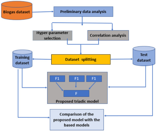
Figure 1.
Proposed triadic ensemble model.
2.1. Data Collection
This research is part of other ongoing research works. In a previous study, an IoT framework was developed to monitor and control a biogas digester status and is considered a data collection tool in this study. The data were collected in three months from March 2023 on a home digester. The dataset contains 3000 records encompassing operational parameters data, such as digester temperature (T), digester pH (pH), moisture level, pH level, and gas volume. The description of the IoT platform and data collection process was reported in our previous study [27]. The temperature is important, as it affects the production rate. The pH level is vital for determining the stability and corrosiveness of the biogas. Gas volume is a factor providing insights into the gas energy content. The moisture level measurement is important, as moisture influences the movement of microorganisms. Table 1 presents an explanation of the variables considered in the proposed biogas prediction model.

Table 1.
Explanatory variables in the biogas prediction model.
In the machine learning modeling process, data pre-processing must be conducted to ensure the accuracy of the model. In a previous study [27], data pre-processing was performed, and rows with both missing and high peak values were substituted with the mean values of all available data. Timestamp values were converted from the 12 h system to the 24 h system using the strftime function from the DateTime library to facilitate the consideration of the time factor.
2.2. Machine Learning Models
In this research, we propose a triadic ensemble machine learning model, which integrates three distinct algorithms: LightGBM, CatBoost, and evolutionary strategy. The model engages supervised machine learning regression models, where a set of input data is employed to predict the output data [28]. The proposed model was compared with existing regression models, namely, random forest, KNN, and decision tree. The most effective model is recommended to predict biogas production. These predicted values can be utilized to optimize biogas plant operations or devise strategies for future biogas production.
2.2.1. K-Nearest Neighbor (KNN)
The KNN algorithm is a machine learning technique used for regression tasks. It relies on the idea that similar data points tend to have similar values. Throughout the training process, the KNN algorithm stores the whole training dataset as a reference to perform predictions, calculating of the distance between the input data point and the trained data by referring to Euclidean distance [29,30].
2.2.2. Random Forest
Random forest is a powerful machine learning (ML) algorithm. It can handle both classification and regression problems. Figure 2 shows how random forest combines the output of multiple decision trees to reach a single result. Its ease of use and flexibility have fueled its adoption. The random forest algorithm is a bagging method expansion that employs both bagging and feature randomness to produce an uncorrelated forest of decision trees [31].
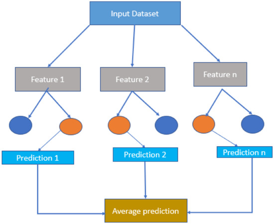
Figure 2.
The random forest model.
2.2.3. Decision Tree
Decision trees (DTs) are a popular supervised learning method that can work for both regression and classification problems. Decision trees build a model that predicts the value of a target variable by inferring basic decision rules from data features. A decision tree is a hierarchical decision support model that displays options and their probable outcomes, including chance occurrences, resource expenses, and utility [32].
2.2.4. Light Gradient-Boosting Machine (LightGBM)
LightGBM, as suggested by Microsoft [33], is an advanced supervised algorithm built on the foundation of gradient-enhanced decision trees. It has found applications in various domains, including medicine [28], economy [34], and agriculture [35]. LightGBM is a gradient-boosting framework that uses tree-based learning algorithms and relies on a loss function that measures the discrepancy between the predicted and the actual values of the target variable [36,37].
where L(Θ) is the loss function that depends on the model parameter Θ. The goal of machine learning is to find the optimal values of Θ that minimize the loss function. F(xᵢ) is the model output or prediction for the input xᵢ. F is a function that maps the input space to the output space and is determined by the model parameter Θ; the sum of all training samples (xᵢ, yᵢ) is denoted by Σ. The loss function l (yᵢ, F(xᵢ)) measures the difference between the predicted value F(xᵢ) and the true value yᵢ. The regularization term Ω(F) is a function of the model output F and penalizes the complexity of the model. Additionally, there is an optional regularization term, Ψ(Θ), which is a function of the model parameter Θ and penalizes the magnitude of the parameters.
2.2.5. Gradient Boosting (CatBoost)
CatBoost is a gradient-boosting framework invented in 2017, with the ability to handle regression features effectively [38]. CatBoost relies on a loss function that measures the discrepancy between the predicted values and the actual values of the target variable. The CatBoost algorithm minimizes the loss function by updating the ensemble in each iteration. As indicated in Equation (2), at the t-th iteration, the predicted value of the ensemble for a specific sample xᵢ is denoted by Ft−1(xᵢ), and the update equation for Fₜ(xᵢ) is:
Fₜ(xᵢ) = Ft−1(xᵢ) + γₜhₜ(xᵢ)
The learning rate γₜ in Equation (2) corresponds to the learning rate for the t-th iteration, while hₜ(xᵢ) represents the prediction made by the t-th decision tree for the sample xᵢ [38,39,40].
2.2.6. Evolutionary Strategy
Evolution strategy is a global optimization algorithm that incorporates stochastic elements, inspired by the biological principle of evolution through natural selection [41]. The evolutionary strategy algorithm optimizes the parameters θ1, θ2, …, θn of model M to minimize the loss function L(M,θ). It generates a population of M models with the random parameters θ1, θ2, …, θN. It evaluates the fitness of each model in the population based on the loss function f(θi) = L(M,θi). Then, it selects the top-performing models. Its selects the top k models from a population, based on their fitness scores [42,43].
Proposed Triadic Ensemble Model
The triadic ensemble model involved the utilization of the synergies of the described base models to enhance their performance and boost their generalization capabilities. The triadic ensemble model learning was broken down into two phases: the training phase of the base models and the training phase of the merged model. During the initial phase, the original dataset was partitioned into a training set and a testing set. The training set was then used for training through k-fold cross-validation. In k-fold cross-validation, the training set was divided into k subsets, with each subset serving as a validation set, while the remaining (k − 1) subsets were utilized for training the model and generating predictions for that specific validation subset. Table 2 indicates the proposed model workflow.
Table 2.
Proposed triadic ensemble workflow.
2.3. Evaluation Metrics
The evaluation metrics used in this paper included RMSE, MAE, and coefficient of determination (R-squared). These metrics are used to assess the performance of regression models. The RMSE measures the average squared difference between predicted and actual values, with a lower RMSE indicating a better fit [44,45]. Similarly, the MAE measures the average absolute difference between predicted and actual values, with a lower MAE also indicating a better fit [46]. The R-squared gauges how well a model fits the data, with a higher R-squared value indicating a better fit. We compared different regression models based on these metrics. The model achieving the lowest RMSE and MAE as well as the highest R-squared was considered the best model for the task. The mathematical formulas are as follows:
coefficient of determination (R2)
root-mean-square error (RMSE)
is the predicted value of the ith sample, and is the corresponding true value for the total samples.
2.4. Hyperparameter Optimization
In machine learning, it is essential to set hyperparameters before initiating the model training process. This is especially important for algorithms like LightGBM, CatBoost, and evolutionary strategy, as in this case, hyperparameters significantly impact each model’s predictive accuracy. This study used hyperparameter optimization techniques to improve the performance of the proposed model. RandomizedSearchCV is a tool used to evaluate hyperparameter computation and improve prediction accuracy. RandomizedSearchCV indicated the following hyperparameters for the LightGBM model:
- Learning rate: [0.01, 0.1];
- Number of estimators: sp_randint(100, 1000);
- Maximum depth: sp_randint(3, 8).
The ‘n_iter’ parameter of RandomizedSearchCV was set to 10, indicating that 10 sets of hyperparameters would be randomly sampled from the identified parameter space. Moreover, the ‘cv’ parameter was set to 5, suggesting that nested 5-fold cross-validation would be used to measure the performance of each hyperparameter arrangement. Once the best hyperparameter configuration was known, the LightGBM model was trained on the entire training dataset using these settings. The trained model was then employed to make predictions on the unknown test dataset. Figure 3 shows how nested 5-fold cross-validation was performed for each iteration; one of the 5 folds was considered a testing dataset.
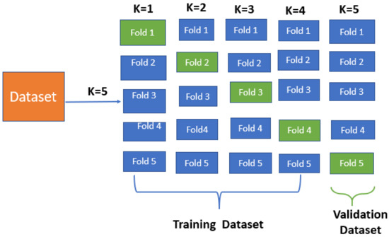
Figure 3.
The 5-fold cross-validation.
3. Results and Discussion
This section details the prediction result obtained from modeling biogas digester environmental data collected from March to May 2023, using the proposed stacking ensemble model. For the performance analysis, the model was compared with other models presented in this study, using performance evaluation metrics such as RMSE, MAE, adjusted R-squared. Additionally, the correlation of different variables was explored in this research.
3.1. Proposed Model Prediction Results
The dataset used in this study comprises 3000 records. These data regard environmental parameters that have an impact on biogas yield. The model was setup to predict the volume of biogas yield in the next hours referring to five input values previously measured (ambient temperature, indoor temperature, moisture, pH level, and time) in the experiment. For selecting the training and testing dataset, the k-fold cross-validation approach was used. We chose k = 5 to balance the computation cost presented by the high value of k and prevent bias caused by k = 3. Among the k-fold cross-validation methods, nested cross-validation was selected to optimize hyperparameter turning on the dataset and reduce bias, and five-fold cross-validation was carried out within each cross-validation. For each iteration, the dataset was divided into four folds (80%) of training and one fold (20%) of testing data. The performance of the models was evaluated using three metrics, as mentioned in Section 2.3. The cross-validation results showed less significant changes using different values of k, as indicated in Table 3.
Table 3.
Model results through the cross-validation test.
3.2. Comparative Analysis of Machine Learning Models
For the performance analysis of the model, the results of the proposed model were compared to those of three machine learning models, i.e., KNN, DT, and RF, using the same five-fold cross-validation on the same dataset. The results from different values of K were computed. Table 4 shows only the average results in terms of R2, RMSE, and MAE values.
Table 4.
Models’ results comparison through cross-validation.
3.2.1. Accuracy of the Model (RMSE and MAE)
The RMSE measures the average distance between the predicted values and the actual values. A lower RMSE indicates better accuracy. The MAE measures the average absolute difference between the predicted values and the actual values. Like the RMSE, a lower MAE suggests better accuracy. The average differences between the predicted values and the actual values for the biogas yield were 0.0040, 0.0055, 0.0062, and 0.0059 for the proposed model and the RF, DT, and KNN models, respectively, whereas the average absolute differences between the predicted values and the actual biogas yield were 0.0024, 0.0044, 0.0049, and 0.0047 for these models, respectively, as presented in Figure 4. Overall, the proposed method demonstrated the highest accuracy with the lowest RMSE and MAE values, followed by the random forest and KNN models, while the decision tree model showed relatively lower accuracy.
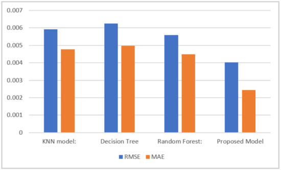
Figure 4.
Comparison of the RMSE and MAE of the different models.
3.2.2. Model Fit (R-Squared)
Figure 5 presents a comparative analysis using R-squared metrics. The graph illustrates that different models had varying R-squared values. The random forest model achieved an R-squared value of 0.6863, indicating that approximately 68.63% of the variance in the target variable could be explained by the model. The decision tree model obtained an R-squared value of 0.6240, indicating that approximately 62.40% of the variance in the target variable could be explained by this model. The KNN model achieved an R-squared value of 0.6540, indicating that approximately 65.40% of the variance in the target variable could be explained by this model. The proposed method obtained the highest R-squared value of 0.7808, indicating that approximately 78.08% of the variance in the target variable could be explained by this model. Overall, the proposed method demonstrated the highest model fit, with the highest R-squared values, indicating that it could better explain the variance in the target variable compared to the other models.
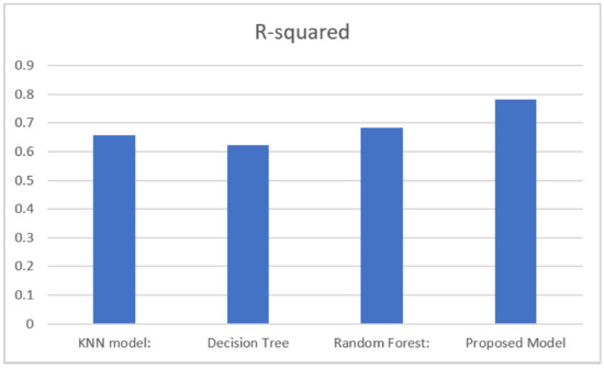
Figure 5.
Comparison of the R-squared values of the different models.
3.3. Variable Importance
Scatterplots offer a valuable visualization of the relationships between various environmental parameters that affect biogas yield. However, it is possible to enhance the design of these diagrams and the information they contain. This could be achieved by providing clearer labels for the axes and, in this study, by reducing the number of the data points reported in Figure 6. The ordinate axis represents the moisture content of the biogas, measured in percentage. A higher percentage indicates a greater amount of moisture in the biogas. On the other hand, the abscissa axis represents the temperature of the biogas, measured in degrees Celsius. A higher temperature indicates a hotter biogas. Each data point on the scatterplot represents a single measurement of moisture and temperature for a specific sample of biogas. The color of the data points represents the gaz_change value for the corresponding sample, with darker shades indicating higher values. Additionally, the size of the data points represents the pH value, with larger points indicating higher values. By analyzing the scatterplot, several observations can be made. Firstly, there is a general trend of increasing moisture content with increasing temperature. Furthermore, the gaz_change value appears to be negatively correlated with the moisture content, suggesting that biogas with higher moisture content tended to have a lower gaz_change value. Lastly, there seems to be a positive correlation between the pH value and the temperature, indicating that biogas with higher temperatures tended to have higher pH values.
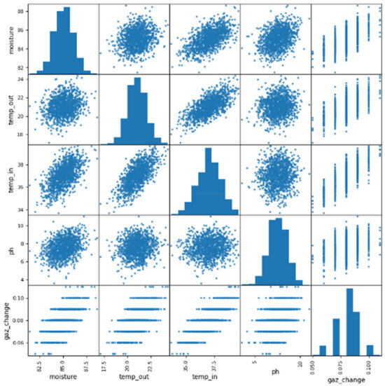
Figure 6.
Comprehensive insights: scatterplot matrix analysis of the biogas dataset.
4. Conclusions
Biogas is one of the promising sources of energy available for local communities due to its characteristics. Recently, biogas operators have been facing several challenges such as a lack of technology to monitor the indoor production process. In the biogas generation process, environmental parameters are among the major factors affecting biogas production. With artificial intelligence (AI) and internet of things (IoT) technology, it is possible to increase biogas yield using an accurate predictive model cooperating with an IoT-based fermentation control system. In prior research, an IoT-based data collection tool was designed to collect environmental data on a home digester. The dataset comprises of indoor and ambient temperature, moisture level, and biogas yield. In this research, we proposed a biogas yield prediction model that guarantees high accuracy by applying a stacking-based learning model. The triadic assembler model combines the LightGBM, CatBoost, and evolutionary strategy models was developed, and compared with other machine learning models. The stacking model outperformed the KNN, RF, and DT models, in terms of RMSE, R2, and MAE metrics, and the proposed model performed the best on both training and testing datasets.
The findings of this research indicated that the triadic ensemble machine learning approach significantly improved biogas yield. The proposed method outperformed all other models, achieving the lowest RMSE and MAE values of 0.0040 and 0.0024, respectively. It also showed the highest R-squared value of 0.7808, indicating superior predictive accuracy and precision. This advancement has significant implications for enhancing biogas plant design and operation, increasing energy output, and addressing environmental challenges.
Due to the testbed scenario, the model must be adapted to the newly collected IoT-based time-series data. Therefore, in the future, it will be important to integrate the transfer learning models and make an intelligent re-training pipeline with the experimented threshold.
Author Contributions
Conceptualization, A.M., L.S., K.J. and K.N.; methodology, A.M., L.S., K.J. and K.N.; software, A.M. and L.S.; validation, A.M., L.S., K.J. and K.N.; formal analysis, A.M., L.S., K.J. and K.N.; investigation, L.S. and K.J.; resources, A.M., L.S. and K.J.; data curation, A.M., L.S. and K.J.; writing—original draft preparation, A.M.; writing—review and editing, L.S., K.J., K.N. and E.H.; visualization, A.M.; supervision, L.S., K.J. and K.N.; project administration, L.S.; funding acquisition, A.M. and L.S. All authors have read and agreed to the published version of the manuscript.
Funding
This research was funded by the African Centre of Excellence on the Internet of Things (ACEIoT), running under the University of Rwanda, College of Science and Technology (UR-CST).
Institutional Review Board Statement
Not applicable.
Informed Consent Statement
Not applicable.
Data Availability Statement
All data used to achieve the research objectives are available at https://aceiot.ur.ac.rw/?Biogas-Dataset, accessed on 12 December 2023, (ACEIoT portal of the University of Rwanda).
Conflicts of Interest
The authors declare no conflict of interest.
References
- National Grid Group. What Is Biogas? Available online: https://www.nationalgrid.com/stories/energy-explained/what-is-biogas (accessed on 19 October 2023).
- Afotey, B.; Sarpong, G.T. Estimation of biogas production potential and greenhouse gas emissions reduction for sustainable energy management using intelligent computing technique. Meas. Sens. 2023, 25, 100650. [Google Scholar] [CrossRef]
- Kang, S.; Kim, G.; Jeon, E.-C. Ammonia Emission Estimation of Biogas Production Facilities in South Korea: Consideration of the Emission Factor Development. Appl. Sci. 2023, 13, 6203. [Google Scholar] [CrossRef]
- Saraswat, M.; Garg, M.; Bhardwaj, M.; Mehrotra, M.; Singhal, R. Impact of variables affecting biogas production from biomass. IOP Conf. Series Mater. Sci. Eng. 2019, 691, 012043. [Google Scholar] [CrossRef]
- Malet, N.; Pellerin, S.; Nesme, T. Agricultural biomethane production in France: A spatially-explicit estimate. Renew. Sustain. Energy Rev. 2023, 185, 113603. [Google Scholar] [CrossRef]
- Bumharter, C.; Bolonio, D.; Amez, I.; Martínez, M.J.G.; Ortega, M.F. New opportunities for the European Biogas industry: A review on current installation development, production potentials and yield improvements for manure and agricultural waste mixtures. J. Clean. Prod. 2023, 388, 135867. [Google Scholar] [CrossRef]
- Sudiartha, G.A.W.; Imai, T.; Mamimin, C.; Reungsang, A. Effects of Temperature Shifts on Microbial Communities and Biogas Production: An In-Depth Comparison. Fermentation 2023, 9, 642. [Google Scholar] [CrossRef]
- Møller, H.B.; Sørensen, P.; Olesen, J.E.; Petersen, S.O.; Nyord, T.; Sommer, S.G. Agricultural Biogas Production—Climate and Environmental Impacts. Sustainability 2022, 14, 1849. [Google Scholar] [CrossRef]
- Gopal, L.C.; Govindarajan, M.; Kavipriya, M.; Mahboob, S.; Al-Ghanim, K.A.; Virik, P.; Ahmed, Z.; Al-Mulhm, N.; Senthilkumaran, V.; Shankar, V. Optimization strategies for improved biogas production by recycling of waste through response surface methodology and artificial neural network: Sustainable energy perspective research. J. King Saud Univ.-Sci. 2021, 33, 101241. [Google Scholar] [CrossRef]
- Induchoodan, T.G.; Haq, I.; Kalamdhad, A.S. Factors affecting anaerobic digestion for biogas production: A review. Adv. Org. Waste Manag. Sustain. Pract. Approaches 2022, 223–233. [Google Scholar] [CrossRef]
- Kunatsa, T.; Zhang, L.; Xia, X. Biogas potential determination and production optimisation through optimal substrate ratio feeding in co-digestion of water hyacinth, municipal solid waste and cow dung. Biofuels 2022, 13, 631–641. [Google Scholar] [CrossRef]
- Artificial Intelligence in Renewable Energy Market Size, Share 2023 to 2032. Available online: https://www.precedenceresearch.com/artificial-intelligence-in-renewable-energy-market (accessed on 20 October 2023).
- Shaw, R.N.; Ghosh, A.; Mekhilef, S.; Balas, V.E. Applications of AI and IOT in Renewable Energy; Elsevier BV: Amsterdam, The Netherlands, 2022; ISBN 9780323916998. [Google Scholar]
- Lyu, W.; Liu, J. Artificial Intelligence and emerging digital technologies in the energy sector. Appl. Energy 2021, 303, 117615. [Google Scholar] [CrossRef]
- Onu, P.; Mbohwa, C.; Pradhan, A. Artificial intelligence-based IoT-enabled biogas production. In Proceedings of the 2023 International Conference on Control, Automation and Diagnosis, ICCAD 2023, Rome, Italy, 10–12 May 2023. [Google Scholar] [CrossRef]
- Yang, Y.; Zheng, S.; Ai, Z.; Jafari, M.M.M. On the Prediction of Biogas Production from Vegetables, Fruits, and Food Wastes by ANFIS- and LSSVM-Based Models. BioMed Res. Int. 2021, 2021, 9202127. [Google Scholar] [CrossRef] [PubMed]
- Kour, V.P.; Arora, S. Particle Swarm Optimization Based Support Vector Machine (P-SVM) for the Segmentation and Classification of Plants. IEEE Access 2019, 7, 29374–29385. [Google Scholar] [CrossRef]
- Meza, J.K.S.; Yepes, D.O.; Rodrigo-Ilarri, J.; Rodrigo-Clavero, M.-E. Comparative Analysis of the Implementation of Support Vector Machines and Long Short-Term Memory Artificial Neural Networks in Municipal Solid Waste Management Models in Megacities. Int. J. Environ. Res. Public Health 2023, 20, 4256. [Google Scholar] [CrossRef] [PubMed]
- Chen, W.-Y.; Chan, Y.J.; Lim, J.W.; Liew, C.S.; Mohamad, M.; Ho, C.-D.; Usman, A.; Lisak, G.; Hara, H.; Tan, W.-N. Artificial Neural Network (ANN) Modelling for Biogas Production in Pre-Commercialized Integrated Anaerobic-Aerobic Bioreactors (IAAB). Water 2022, 14, 1410. [Google Scholar] [CrossRef]
- Chiu, M.-C.; Wen, C.-Y.; Hsu, H.-W.; Wang, W.-C. Key wastes selection and prediction improvement for biogas production through hybrid machine learning methods. Sustain. Energy Technol. Assess. 2022, 52, 102223. [Google Scholar] [CrossRef]
- Renard, B.; Kavetski, D.; Kuczera, G.; Thyer, M.; Franks, S.W. Understanding predictive uncertainty in hydrologic modeling: The challenge of identifying input and structural errors. Water Resour. Res. 2010, 46, W05521. [Google Scholar] [CrossRef]
- Amina, M.K.; Chithra, N.R. Predictive uncertainty assessment in flood forecasting using quantile regression. H2Open J. 2023, 6, 477–492. [Google Scholar] [CrossRef]
- Gupta, A.; Jain, V.; Singh, A. Stacking Ensemble-Based Intelligent Machine Learning Model for Predicting Post-COVID-19 Complications. New Gener. Comput. 2022, 40, 987–1007. [Google Scholar] [CrossRef]
- Meharie, M.G.; Mengesha, W.J.; Gariy, Z.A.; Mutuku, R.N. Application of stacking ensemble machine learning algorithm in predicting the cost of highway construction projects. Eng. Constr. Archit. Manag. 2022, 29, 2836–2853. [Google Scholar] [CrossRef]
- Li, J.; Zhang, L.; Li, C.; Tian, H.; Ning, J.; Zhang, J.; Tong, Y.W.; Wang, X. Data-Driven Based In-Depth Interpretation and Inverse Design of Anaerobic Digestion for CH4-Rich Biogas Production. ACS ES&T Eng. 2022, 2, 642–652. [Google Scholar] [CrossRef]
- Zhang, Y.; Zhao, Y.; Feng, Y.; Yu, Y.; Li, Y.; Li, J.; Ren, Z.; Chen, S.; Feng, L.; Pan, J.; et al. Novel Intelligent System Based on Automated Machine Learning for Multiobjective Prediction and Early Warning Guidance of Biogas Performance in Industrial-Scale Garage Dry Fermentation. ACS ES&T Eng. 2023. [Google Scholar] [CrossRef]
- Mukasine, A.; Sibomana, L.; Jayavel, K.; Nkurikiyeyezu, K.; Hitimana, E. Correlation Analysis Model of Environment Parameters Using IoT Framework in a Biogas Energy Generation Context. Futur. Internet 2023, 15, 265. [Google Scholar] [CrossRef]
- Mapundu, M.T.; Kabudula, C.W.; Musenge, E.; Olago, V.; Celik, T. Explainable Stacked Ensemble Deep Learning (SEDL) Framework to Determine Cause of Death from Verbal Autopsies. Mach. Learn. Knowl. Extr. 2023, 5, 1570–1588. [Google Scholar] [CrossRef]
- Bansal, M.; Goyal, A.; Choudhary, A. A comparative analysis of K-Nearest Neighbor, Genetic, Support Vector Machine, Decision Tree, and Long Short Term Memory algorithms in machine learning. Decis. Anal. J. 2022, 3, 100071. [Google Scholar] [CrossRef]
- KNN Algorithm|Latest Guide to K-Nearest Neighbors. Available online: https://www.analyticsvidhya.com/blog/2018/03/introduction-k-neighbours-algorithm-clustering/ (accessed on 29 November 2023).
- Atmanspacher, H.; Martin, M. Correlations and How to Interpret Them. Information 2019, 10, 272. [Google Scholar] [CrossRef]
- Decision Tree Algorithm—A Complete Guide—Analytics Vidhya. Available online: https://www.analyticsvidhya.com/blog/2021/08/decision-tree-algorithm/ (accessed on 29 November 2023).
- Ke, G.; Meng, Q.; Finley, T.; Wang, T.; Chen, W.; Ma, W.; Ye, Q.; Liu, T.Y. LightGBM: A Highly Efficient Gradient Boosting Decision Tree. Adv. Neural Inf. Process Syst. 2017, 30. Available online: https://github.com/Microsoft/LightGBM (accessed on 28 October 2023).
- Wang, D.-N.; Li, L.; Zhao, D. Corporate finance risk prediction based on LightGBM. Inf. Sci. 2022, 602, 259–268. [Google Scholar] [CrossRef]
- Li, Z.; Wang, W.; Ji, X.; Wu, P.; Zhuo, L. Machine learning modeling of water footprint in crop production distinguishing water supply and irrigation method scenarios. J. Hydrol. 2023, 625, 130171. [Google Scholar] [CrossRef]
- Zhou, Y.; Wang, W.; Wang, K.; Song, J. Application of LightGBM Algorithm in the Initial Design of a Library in the Cold Area of China Based on Comprehensive Performance. Buildings 2022, 12, 1309. [Google Scholar] [CrossRef]
- How LightGBM Algorithm Works—ArcGIS Pro|Documentation. Available online: https://pro.arcgis.com/en/pro-app/latest/tool-reference/geoai/how-lightgbm-works.htm (accessed on 23 October 2023).
- How CatBoost Algorithm Works—ArcGIS Pro|Documentation. Available online: https://pro.arcgis.com/en/pro-app/latest/tool-reference/geoai/how-catboost-works.htm (accessed on 23 October 2023).
- Xiang, W.; Xu, P.; Fang, J.; Zhao, Q.; Gu, Z.; Zhang, Q. Multi-dimensional data-based medium- and long-term power-load forecasting using double-layer CatBoost. Energy Rep. 2022, 8, 8511–8522. [Google Scholar] [CrossRef]
- Wang, D.; Qian, H. CatBoost-Based Automatic Classification Study of River Network. ISPRS Int. J. Geo-Inf. 2023, 12, 416. [Google Scholar] [CrossRef]
- Beyer, H.-G.; Schwefel, H.-P. Evolution strategies—A comprehensive introduction. Nat. Comput. 2002, 1, 3–52. [Google Scholar] [CrossRef]
- Wang, Y.; Li, T.; Liu, X.; Yao, J. An adaptive clonal selection algorithm with multiple differential evolution strategies. Inf. Sci. 2022, 604, 142–169. [Google Scholar] [CrossRef]
- Lange, R.T. evosax: JAX-Based Evolution Strategies. In Proceedings of the GECCO 2023 Companion—2023 Genetic and Evolutionary Computation Conference Companion, Lisbon Portugal, 15–19 July 2023; pp. 659–662. [Google Scholar] [CrossRef]
- Performance Metrics in Machine Learning [Complete Guide]—Neptune.Ai. Available online: https://neptune.ai/blog/performance-metrics-in-machine-learning-complete-guide (accessed on 29 November 2023).
- Evaluation Metrics|12 Must-Know ML Model Evaluation Metrics. Available online: https://www.analyticsvidhya.com/blog/2019/08/11-important-model-evaluation-error-metrics/#Root_Mean_Squared_Error_(RMSE) (accessed on 29 November 2023).
- Metrics to Evaluate your Machine Learning Algorithm|by Aditya Mishra|Towards Data Science. Available online: https://towardsdatascience.com/metrics-to-evaluate-your-machine-learning-algorithm-f10ba6e38234 (accessed on 29 November 2023).
Disclaimer/Publisher’s Note: The statements, opinions and data contained in all publications are solely those of the individual author(s) and contributor(s) and not of MDPI and/or the editor(s). MDPI and/or the editor(s) disclaim responsibility for any injury to people or property resulting from any ideas, methods, instructions or products referred to in the content. |
© 2024 by the authors. Licensee MDPI, Basel, Switzerland. This article is an open access article distributed under the terms and conditions of the Creative Commons Attribution (CC BY) license (https://creativecommons.org/licenses/by/4.0/).