Abstract
This study focuses on using machine learning techniques to accurately predict the generated power in a two-stage back-pressure steam turbine used in the paper production industry. In order to accurately predict power production by a steam turbine, it is crucial to consider the time dependence of the input data. For this purpose, the long-short-term memory (LSTM) approach is employed. Correlation analysis is performed to select parameters with a correlation coefficient greater than 0.8. Initially, nine inputs are considered, and the study showcases the superior performance of the LSTM method, with an accuracy rate of 0.47. Further refinement is conducted by reducing the inputs to four based on correlation analysis, resulting in an improved accuracy rate of 0.39. The comparison between the LSTM method and the Willans line model evaluates the efficacy of the former in predicting production power. The root mean square error (RMSE) evaluation parameter is used to assess the accuracy of the prediction algorithm used for the generator’s production power. By highlighting the importance of selecting appropriate machine learning techniques, high-quality input data, and utilising correlation analysis for input refinement, this work demonstrates a valuable approach to accurately estimating and predicting power production in the energy industry.
1. Introduction
Advancements in artificial intelligence (AI) techniques offer a new approach for predicting power generation in steam turbines, bypassing the need for traditional mathematical and thermodynamic models. The techniques presented in the field of learning from data can be classified into two categories: supervised learning and unsupervised learning. In supervised learning techniques, the model is trained using labelled data. Usually, a classification process is utilised for this purpose. On the other hand, for unsupervised learning, a model is trained through an existing technique such as clustering on the non-labelled data. In addition, the type of data examined is very influential in choosing a learning method. Some types of data do not have time continuity, and it is possible to shuffle the data for the test, train, and validation operations. However, in some cases, there is a temporal connection between each data line and the next line due to the time gap and the data being sequential. As such, if the data lines are moved, meaningful relational information is lost. In this case, especially where there is a time dependency between records, it is recommended to use special techniques such as recurrent neural networks (RNN), convolutional neural networks (CNN), and long short-term memory (LSTM) [1]. In this research, an attempt is made to forecast the power production of a two-stage back-pressure steam turbine generator using various input parameters, utilising the LSTM method. The organisation of this study can be outlined as follows:
- In Section 2, previous research studies that have utilised machine learning methods to predict industry-related parameters are examined and evaluated.
- Section 3 describes the framework and methodology employed in this study.
- Section 4 explains the Willans line model, which is used to estimate generator power by calculating enthalpy, entropy, and work transfer based on thermodynamic principles. The model relies on these calculations to predict power generation.
- In Section 5, a thorough assessment of the outcomes is conducted, including a comparison of the projections with the results obtained through the Willans line model.
- In Section 6, the findings are appraised, emphasising the significance of using machine learning models, particularly LSTM, within the context of various industries.
2. LSTM and Energy Systems Background
The previous work done in this research field can be examined from two perspectives. Firstly, the development of machine learning methods using the input data to create a model, and secondly, the use of that model for achieving the required goal. This section provides a summary of various research studies carried out in the past that have achieved different goals in the field of energy systems. These goals can be broadly categorised into system power output prediction, error detection, performance degradation and modelling, and environmental effects. The studies were conducted on different types of energy systems, such as photovoltaic solar panels, wind turbines, and gas and oil energy systems, with the majority focusing on the latter. Notably, most past research studies have employed the long-short-term memory (LSTM) method to predict the production capacity of energy systems. Some studies have also combined the LSTM method with other techniques, such as the convolutional neural network (CNN) method [2]. The effectiveness of these methods depends on the quality of the input data used; for instance, the time interval of the input data can significantly impact the performance of the system.
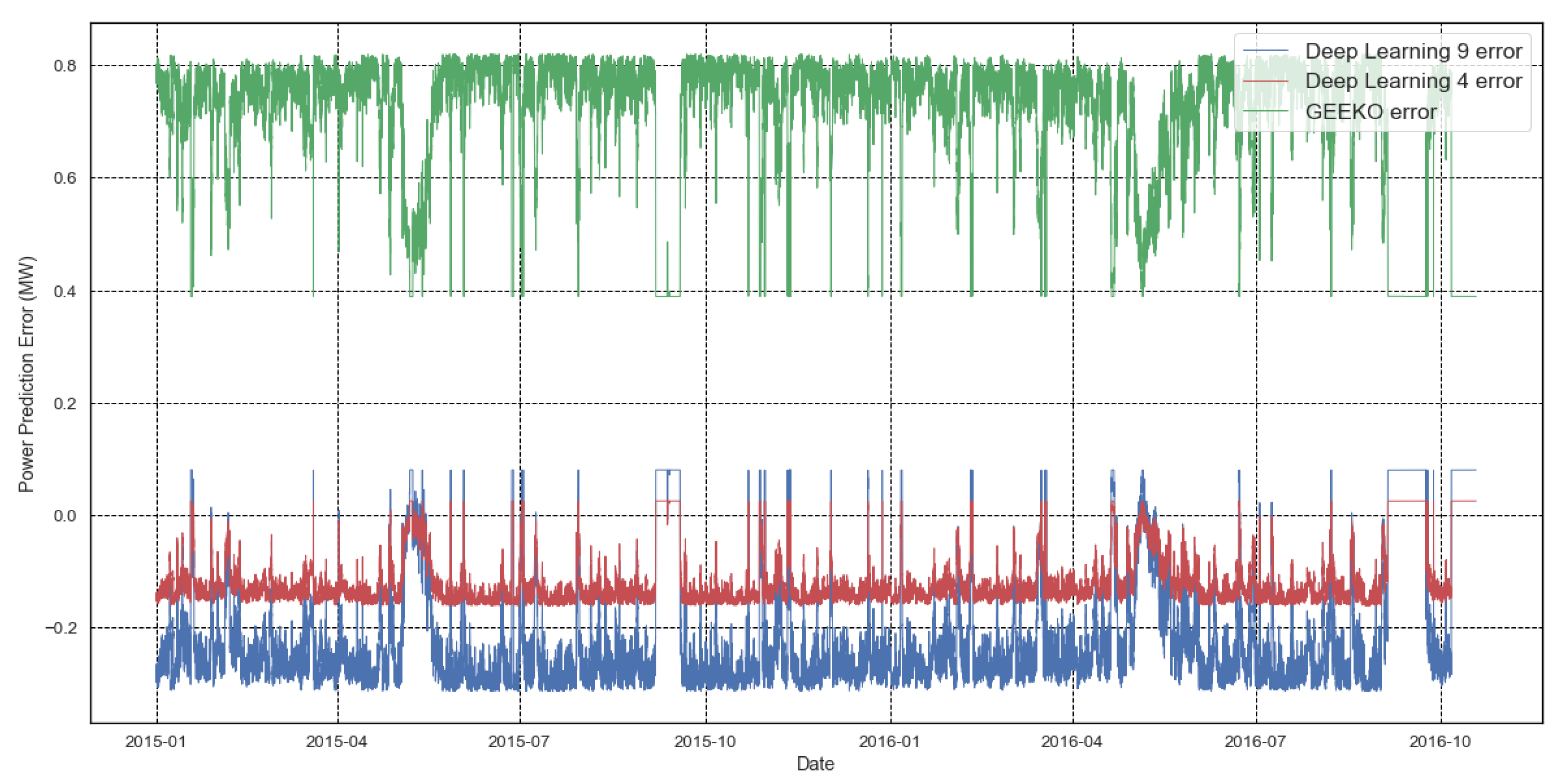
To provide further insights into the different techniques used in these studies, a selection of relevant articles has been chosen for comparison and in-depth examination. Table 1 presents a summary of these studies, including the year of publication, the specific methods employed, the type of case study, and the primary aims, such as power and electricity prediction, fault detection, and environmental impact. As depicted in the table, the energy systems examined can be classified into two overarching categories: oil and gas energy production systems, which include the use of steam turbines within this category, and the second category comprising renewable energy systems. Notably, the research conducted within the first group exhibits a well-balanced distribution and primarily focuses on predicting the lifespan errors and degradation patterns and ultimately forecasting the output power of these system types. On the other hand, with respect to renewable energy systems, as indicated in Table 1, given the inherent instability of such resources, the primary emphasis has been on accurately forecasting the production capacity. Throughout these research endeavors, the predominant methods employed have been LSTM, followed by the combination of LSTM with various other techniques, and ultimately, the utilization of the multi-layer perceptron (MLP) [3] method.
However, one persistent challenge that remains in this field is the intelligent selection of appropriate input variables and suitable architectural configurations to achieve predictions with minimal errors. This necessitates an ongoing effort to refine the choice of input features and the architectural design in order to enhance the accuracy and reliability of predictions in the realm of energy system analysis.
Previous research has utilised a range of software platforms, including MATLAB software in some cases [4], WEKA software in a few cases [5], and predominantly the Python platform [2]. Furthermore, in the context of the research described in this paper, the Python platform was employed for implementing both the LSTM and Willans line models [6].

Table 1.
Summary of most recent learning models focusing on LSTM in energy systems.
Table 1.
Summary of most recent learning models focusing on LSTM in energy systems.
| Reference | Year | Method | Type of Case Study | Aim | |||||
|---|---|---|---|---|---|---|---|---|---|
| Oil/Gas Systems | Wind Energy Systems | Solar Energy Systems | Power Prediction | Fault Detection | Performance Modelling | Environmental Impact | |||
| Nikpey et al. [7] | 2013 | Multi-Layer Perceptron (MLP) | √ | √ | |||||
| Wu et al. [8] | 2016 | LSTM | √ | √ | |||||
| Roni et al. [4] | 2017 | MLP | √ | √ | |||||
| Talaat et al. [9] | 2018 | MLP | √ | √ | |||||
| Zhang et al. [10] | 2018 | LSTM | √ | √ | |||||
| Cao et al. [11] | 2018 | LSTM | √ | √ | |||||
| Zhang et al. [12] | 2019 | Gaussian Mixture Model (GMM) + LSTM | √ | √ | |||||
| Jung et al. [13] | 2019 | LSTM | √ | √ | |||||
| Gao et al. [14] | 2019 | LSTM | √ | √ | |||||
| Adams et al. [15] | 2020 | SVM | √ | √ | |||||
| Arriagada et al. [16] | 2020 | MLP | √ | √ | |||||
| Yongsheng et al. [17] | 2020 | Extreme Learning Machine (ELM) + LSTM | √ | √ | |||||
| Wang et al. [18] | 2020 | Time correlation modification + LSTM | √ | √ | |||||
| Mei et al. [19] | 2020 | LSTM | √ | √ | |||||
| Yuvaraju et al. [20] | 2020 | LSTM | √ | √ | |||||
| Cao et al. [21] | 2021 | LSTM | √ | √ | |||||
| Bai et al. [22] | 2021 | LSTM | √ | √ | |||||
| Alsabban et al. [23] | 2021 | LSTM | √ | √ | |||||
| Dong et al. [24] | 2021 | LSTM+ Gaussian mixture mode (GMM) | √ | √ | |||||
| Zhang et al. [25] | 2021 | CNN + LSTM | √ | √ | |||||
| Zhou et al. [26] | 2021 | Lower and upper bound estimation (LUBE) + LSTM | √ | √ | |||||
| Kong et al. [27] | 2022 | LSTM | √ | √ | |||||
| Ijaz et al. [28] | 2022 | LSTM | √ | √ | |||||
| Zhang et al. [29] | 2023 | LSTM | √ | √ | |||||
| Kabengele et al. [30] | 2023 | MLP | √ | √ | |||||
This present study focuses on the prediction of the power output of a two-stage back-pressure steam turbine generator used in the paper production industry. To this end, a simple and computationally efficient LSTM method has been utilised, contrasting with the hybrid deep learning method reported in [4]. The use of machine learning algorithms is particularly relevant in this study, as thermodynamic models used to estimate production power are often time-consuming and require numerous constants for calculation. The predicted results are compared with those obtained from the thermodynamic model, providing an evaluation of the LSTM method’s performance and potential advantages.
3. Resources and Techniques
This section delves into three key aspects: the framing of the problem in this case study, the exploration of data necessary for developing a solution, and the presentation of the technique utilised for predicting power production.
3.1. Description of an Industrial Process
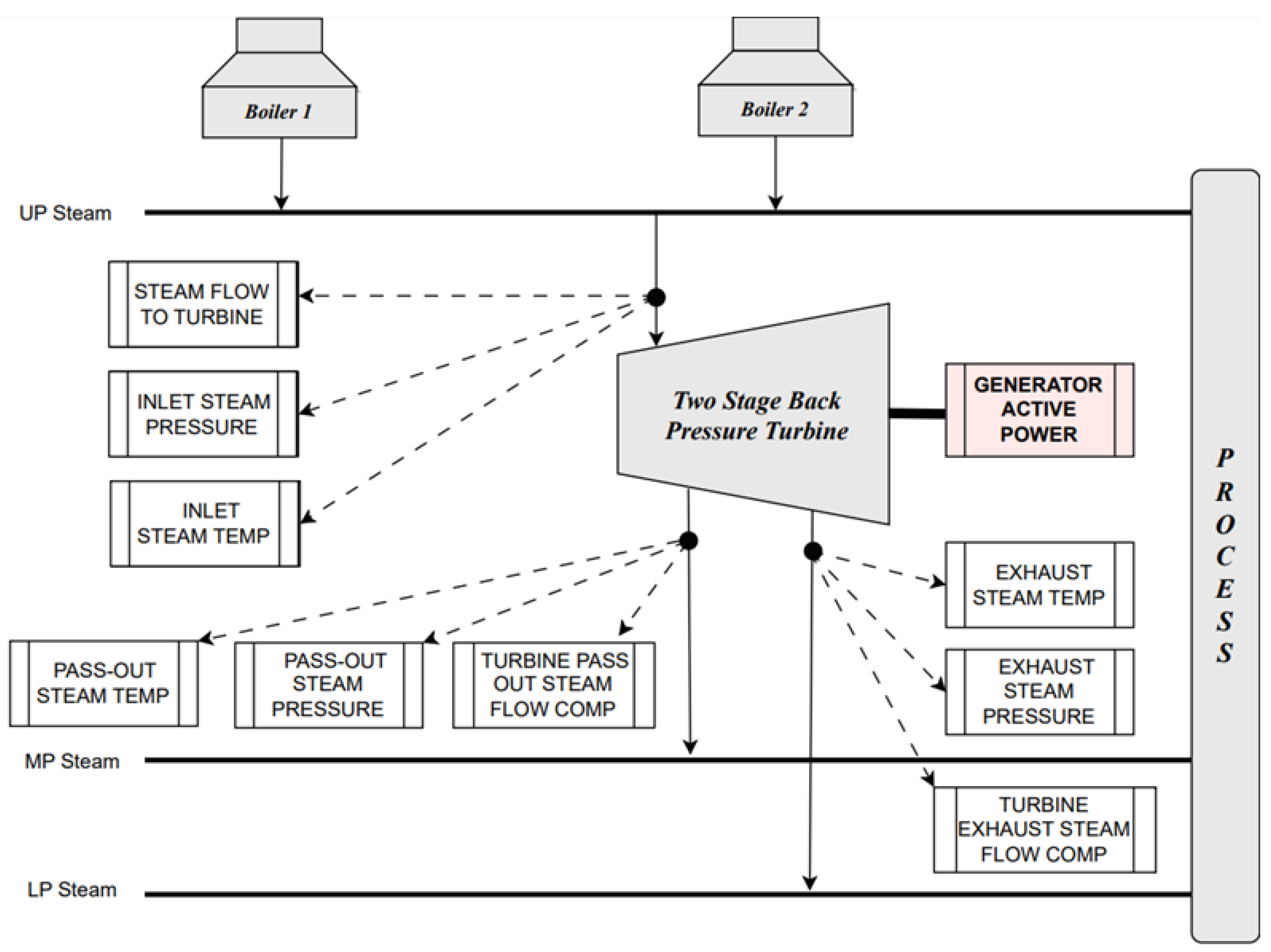
For this research, a two-stage steam turbine at a Kraft Pulp and Paper Mill has been used as a case study (see Figure 1). The power production of this steam turbine is approximately 40 MW. An hourly time-series dataset covering 22 months has been obtained from the industry in order to estimate the output power with high accuracy, low computational complexity, and low execution overhead compared to the Willans line model. Figure 1 shows the inputs and outputs of the model.

Figure 1.
Overview of the process and its inputs and output.
Data have been recorded at 10-min intervals, but there are gaps, with some samples missing. To address this issue, linear interpolation was utilised to fill these gaps. To improve the accuracy of predicting generator active power, the system employs an LSTM model.
3.2. Materials and Methods
Hochreiter and Schmidhuber introduced the LSTM neural networks in 1997 [1], and the concept has since undergone numerous improvements by various individuals. Although LSTM networks are a relatively old technique, they are used in a wide range of applications and are still popular, as shown in Figure 2, which illustrates the utilisation of artificial intelligence techniques in a multitude of research studies conducted in the period spanning from 2016 to 2022. It is evident that in this timeframe, there has been a notable prevalence of LSTM as the primary technique employed, closely followed by the gated recurrent unit (GRU) [31] technique during the initial stages. These two techniques have been employed more frequently in comparison with other methodologies, as shown by the graph.

Figure 2.
Recent usage of neural networks reported in the literature [32].
LSTM neural networks are categorised as a specific type of recursive neural network (RNN), designed to effectively capture and model long-term temporal dependencies within the output data. By incorporating memory cells and gating mechanisms, LSTMs can retain and selectively update information over extended sequences, enabling them to effectively handle and exploit the intricacies of time-dependent patterns present in the data. This distinguishing feature sets LSTMs apart from traditional RNNs, allowing them to excel in tasks such as time series analysis, where capturing long-range dependencies is crucial for accurate predictions and insightful analysis.
An indication of the range of applications where LSTM methods have been utilised is shown in Figure 3. Primarily, this approach has been prominent for time series data analysis, where the data exhibit temporal interdependencies. Further, LSTM models have also found application in the domains of language modelling and sentiment analysis.
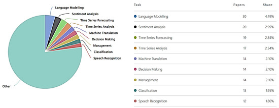
Figure 3.
The extent to which LSTM neural networks have been used in different fields [32].
The research described here considers different inputs as shown in Figure 4, with an architecture comprising 50 neurons in LSTM layers having an activation “Relu” [33] function. The “ADAM” optimizer [34] has been included in the model to minimise errors. The model was trained using 40% of the available data, and the remaining 60% were utilised to test the model.
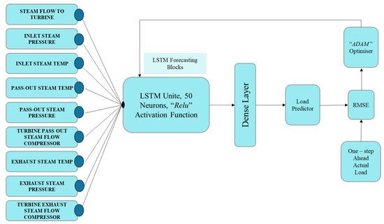
Figure 4.
Steam turbine power prediction model architecture.
The selection of evaluation parameters is also an important issue in the application of machine learning. When the purpose of machine learning is to predict the value of a specific variable, the evaluation parameters that are usually used are mean absolute percentage error (MAPE), root mean square error (RMSE), mean percentage error (MPE), and absolute percentage error (APE) [35]. The MPE measures the average difference between predicted and true values over N samples using Equation (1) below. The RMSE measures the square root of the average of the squared differences between predicted and true values over N samples using Equation (2).
The APE of each sample is calculated using Equation (3), which measures the absolute percentage difference between predicted and true values. The MAPE is then calculated by averaging the APEs over N samples using Equation (4). By selecting appropriate evaluation parameters, machine learning models can be optimised to improve the accuracy of their predictions.
3.3. Correlation Analysis
One of the key aspects of correlation analysis is exploring the interdependence between different parameters and their influence on the output. Correlation analysis is a crucial tool in several fields, including economics, as it can offer significant insights into the connection between variables. This analysis involves calculating the correlation variable using a specific relationship between the parameters, as shown in Equation (5), resulting in a value between zero and a positive one. When the value is closer to one, this implies that the target variable is significantly affected by other variables under consideration, and vice versa. A zero coefficient denotes an absence of correlation between the variables.
Considering the mathematical relationship shown in Equation (5), a thorough evaluation and calculation of the correlations was conducted across all parameters. This assessment aimed to discern the extent of interdependence and mutual influence between the parameters. In Figure 5, the correlation between each pair of parameters is displayed using distinct colors. To provide a better understanding of the intricate relationships among various parameters, Figure 6 depicts the magnitude of influence that each parameter exerts on the others if the correlation factor between them is greater than 0.8. Upon careful examination of this diagram, it becomes apparent that when the correlation parameter surpasses a value of 0.8, a linear equation is deemed suitable for capturing the underlying relationship. This line of best fit is employed to describe the connection between the two relevant parameters, and the corresponding equation is then presented for reference and analysis.
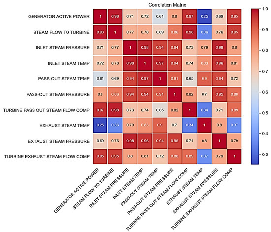
Figure 5.
Correlation matrix of input data from the steam turbine.
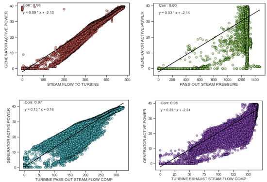
Figure 6.
Correlation analysis of steam flow to turbine, pass−out steam pressure, turbine pass out steam flow comp, and turbine exhaust steam flow comp with output parameter, with correlation factor bigger than 0.8.
Furthermore, in the scope of this research, the focal point revolves around the generator’s production power, which is considered the ultimate output. Considering this, a careful selection process was carried out to identify pertinent inputs for the second model under evaluation. Specifically, as shown originally in Figure 6, four parameters—steam flow to turbine, pass-out steam pressure, turbine pass-out steam flow compressor, and turbine exhaust steam flow compressor—were found to exhibit a correlation parameter exceeding 0.8 when compared with the output parameter. Consequently, these four parameters were designated as inputs for the second model in this study, as their influential impact on the output power warranted further investigation and analysis.
4. Willans Line Model and Equations for Power Generation Estimation
The Willans line, a concept in steam turbine engineering, serves as a guiding principle in the evaluation of the two-stage back-pressure steam turbine. Developed by Robert Willans, this graphical representation provides essential insights into the efficiency and performance of the turbine across varying operating conditions [36]. The line establishes an idealised correlation between power output and steam consumption for an isentropic turbine. By comparing the actual power generated with mass flow to this theoretical line, a clear understanding of the turbine’s real-world efficiency is gained [36]. The Willans line also aids in identifying the most efficient operating range, where the turbine achieves optimal power output while conserving steam. It is a critical tool for ensuring our steam turbine operates at its highest efficiency, minimising resource consumption, and maximising power generation.
The thermodynamic model employed in this study utilises the Willans line to estimate the generated power of the generator. The calculations are performed using the “CoolProp” library [37], which provides functions to calculate properties such as enthalpy and entropy of the working fluid. The model considers multiple stages of the turbine, including the high-pressure stage (HPS) and the low-pressure stage (LPS).
In the implemented approach, the “PropsSI” function is used to calculate the enthalpy and entropy of the working fluid based on the given temperature and pressure values. These calculations are performed for the HPS stage, and the resulting values are stored. Similarly, the enthalpy of the medium-pressure stage is derived from the HPS entropy using the entropy–enthalpy relationship, and the entropy of the MPS stage is calculated directly. The work transfer between stages is then computed by multiplying the mass flow rates with the differences in enthalpy. This results in the calculation of the work done in the HPS stage and the LPS stage. The total generated power is obtained by summing the individual work transfers.
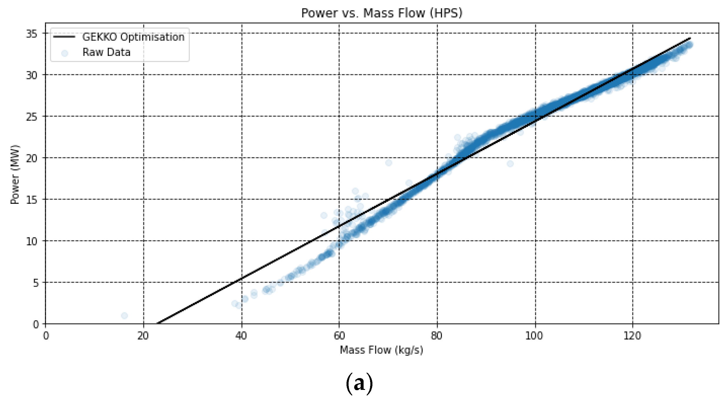
To optimise the regression of the raw data, the “GEKKO” library [38] is utilized. It provides capabilities for regression analysis and optimization. The implemented model performs regression analysis using the “GEKKO” library to find the best-fit parameters for the power-mass flow relationship. The resulting parameters are used to plot the regression lines.
Figure 7 shows the different turbine stages, specifically comparing the modelled Willans line with the raw data. These plots show the performance of the turbine under varying operating conditions, as well as how closely the model matches the raw data. For both the higher-pressure stage (a) and the lower-pressure stage (b), there is a close correlation at higher mass flows, but this begins to deviate away at lower pressures. While this type of Willans line can be useful for estimating the work generation under various loads, it is difficult to validate the outputs of these individual stages, as often multi-stage turbines operate with single, common generators, meaning that individual power values for stages are not available but rather only the overall power.
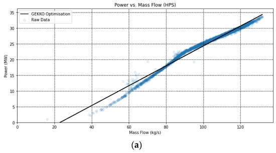
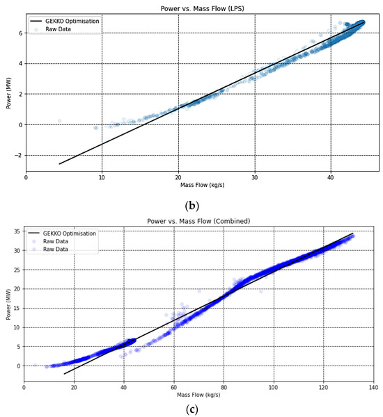
Figure 7.
Steam flow vs power output: (a) High-pressure stage (HPS), (b) low-pressure stage (LPS), (c) combined HPS and LPS.
5. Results
This section presents the results obtained from the implementation of the model, providing a comprehensive understanding of its performance. Figure 8 depicts the outcomes, revealing that a significant proportion of the predicted points generated by the model, whether from the testing data or the training data, coincide with the actual data points. This alignment suggests a minimal level of error between the model’s predictions and the real data, thus indicating the efficacy of the model.
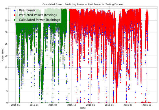
Figure 8.
Comparing real and predicted points of the steam turbine power prediction model.
Prior to arriving at this stage, an extensive investigation was conducted using sensitivity analysis to develop two models, each comprising four inputs. To facilitate comparative analysis, an additional model was constructed based on Willans line equations.
Figure 8 provides insight into the construction process of these models, shedding light on the various steps involved. Remarkably, the measured real power points, symbolised by blue dots, exhibit a striking alignment with both the green points of the training data and the red points representing the testing data. This alignment serves as a demonstration of the performance of the initial model, which consists of nine inputs. Supporting this observation, Table 2 presents the evaluation parameter values for both the training and testing data, with the training data showing a lower RMSE value, aligning with the anticipated outcomes. The fact that these numbers are less than 0.5 shows the better performance of this model than other research with the same purpose [21,30,39,40]. Upon comparing the two outcomes, it was found that the accuracy of the model is better for the training data than the testing data. The reason for this is that the model was trained using this training data and will naturally perform better with this data.

Table 2.
Root Mean Square Error (RMSE) factor for output of the model for testing and training data.
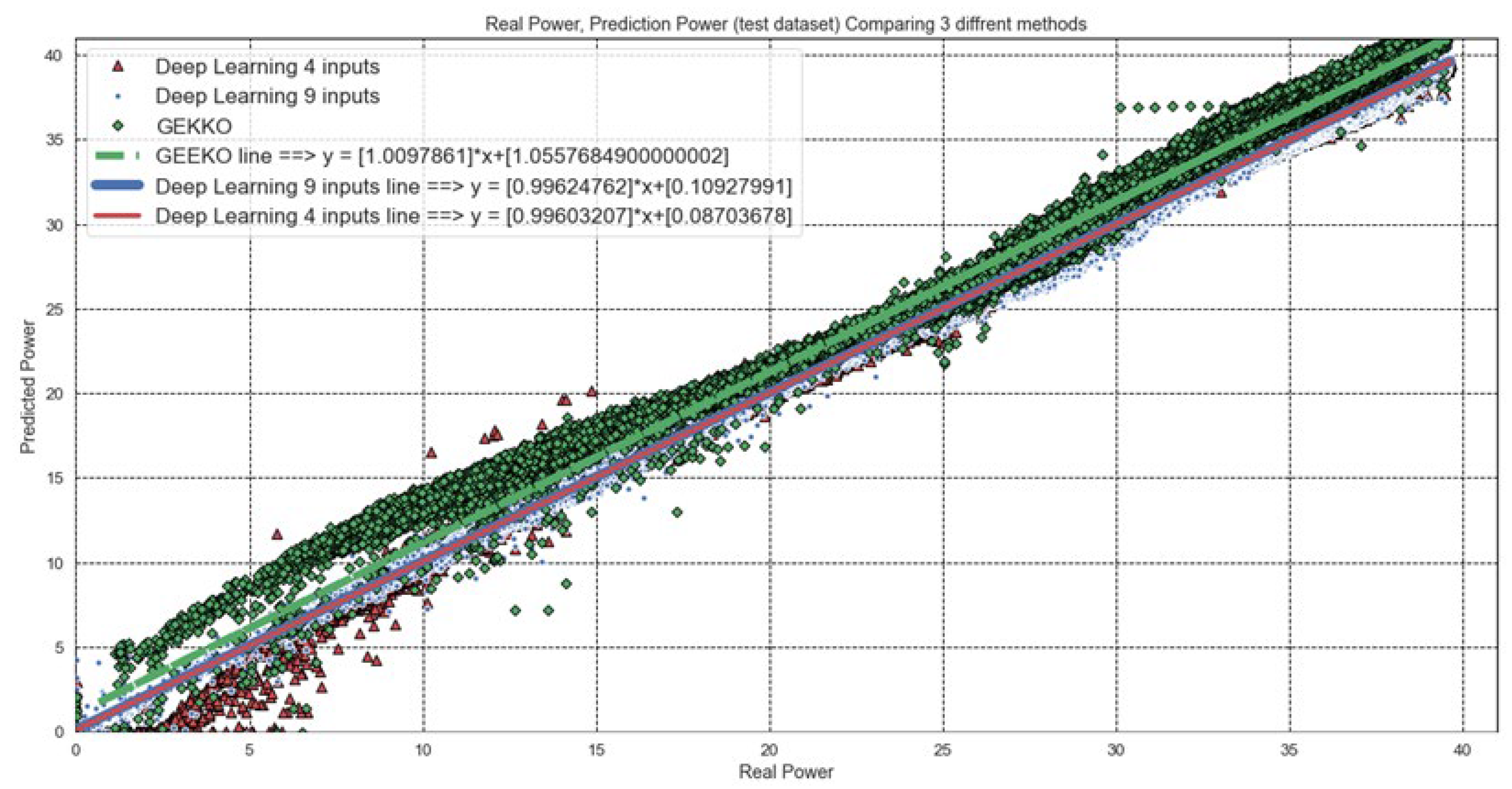
The following section provides a comparative analysis of the results obtained from the three models, which are presented in Figure 9. This graph illustrates the predicted power in relation to the actual power. An ideal model would exhibit a linear relationship with a slope of one and a width of zero, signifying a perfect correspondence between the predicted and actual power values. Considering Figure 9, it becomes evident that both the four-input and nine-input models surpass the performance of the Willans line model. Furthermore, a detailed examination comparing the four-input and nine-input models reveals that the former displays a narrower dispersion, indicative of its superior performance and precision. As illustrated in Figure 9, the line produced by the Willans line model shows a marginal variance from the lines generated by the deep learning model. This discrepancy arises from the fact that approximately 80% of the input data exhibits a power output surpassing 22 MW, exerting a substantial impact on the accuracy of the model derived from the Willans line. Hence, the resultant line is represented as a dashed line in regions where the power output is less than 22 MW.

Figure 9.
Comparison of actual power and predicted power for three models consisting of: Willans line model, nine-input prediction model, and four-input prediction model.
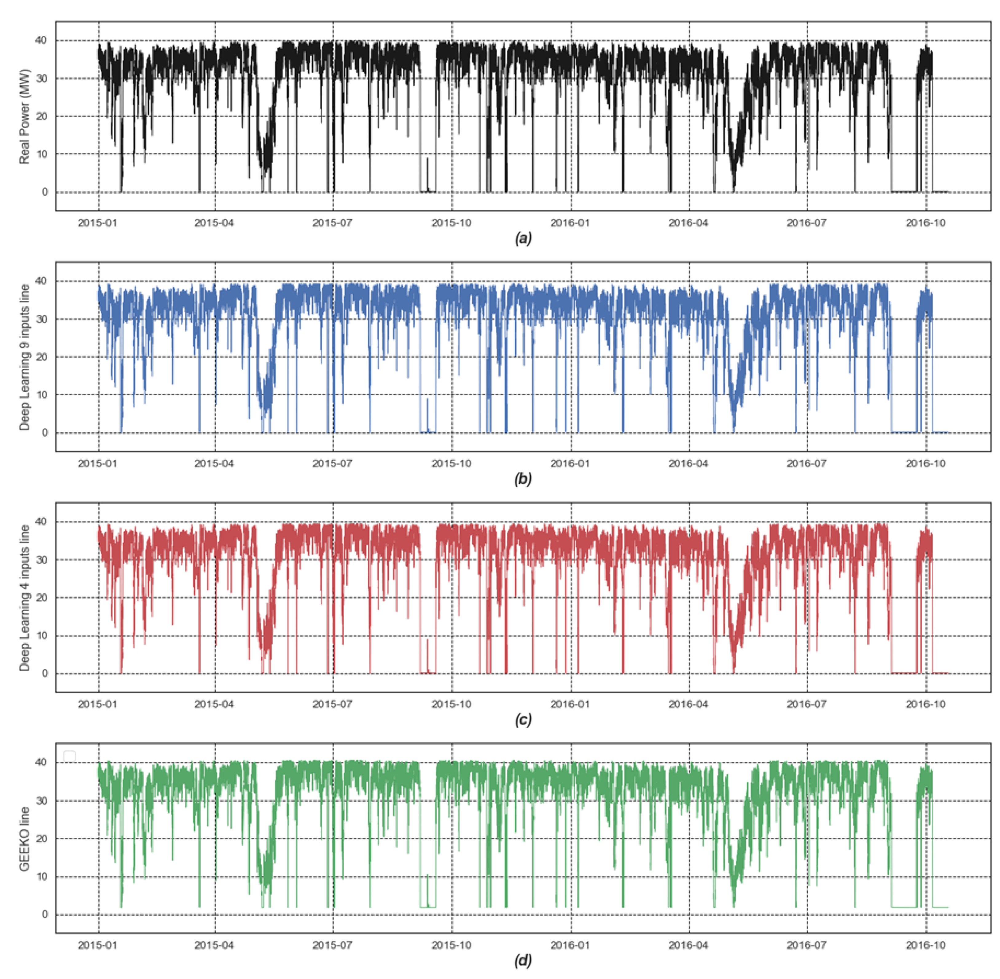
Further insights into the predicted power levels, taking into consideration the dates of data collection, are provided in Figure 10. Notably, the predicted powers depicted in the three charts demonstrate a high degree of consistency, with minimal disparities observed among them. To augment these findings, Figure 11 portrays the individual error magnitudes for each model, serving as additional evidence to reinforce the earlier explanations. This diagram further substantiates the notion that the four-input model outperforms both the nine-input model and the Willans line model, firmly establishing its favourable performance ranking.
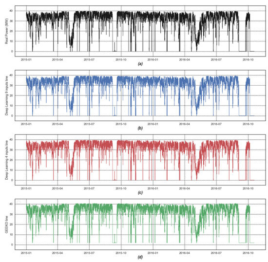
Figure 10.
Comparison of actual power (a) and predicted power for three models consisting of: nine-input prediction model (b), four-input prediction model (c), and Willans line model (d) according to data collection time.
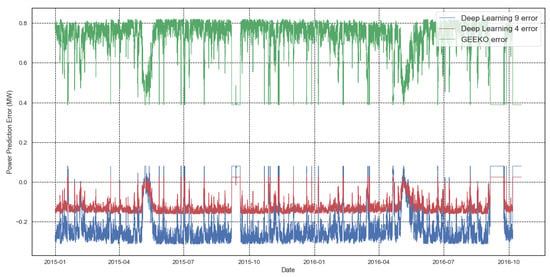
Figure 11.
Individual error magnitudes for each model.
6. Conclusions and Perspectives
The study described here demonstrates that the use of long short-term memory (LSTM), a machine learning algorithm, shows superior performance in predicting the power production of steam turbines than the conventional thermodynamic models. The results obtained from the comparison of LSTM and Willans line models, evaluated using the root mean square error (RMSE) metric, highlight the superior forecasting accuracy of the LSTM approach. Initially employing 9 inputs, the LSTM method achieved an RMSE of 0.47; however, by leveraging correlation analysis and refining the input set to 4 inputs, an even lower RMSE of 0.39 was attained. This study provides evidence for the efficacy of using machine learning algorithms and artificial intelligence to accurately predict desired system performance in various industries.
Moreover, the study highlights the importance of choosing the appropriate machine learning technique based on the type of data examined. In cases where there is time dependence between data lines, techniques such as LSTM that consider the time dependence of input data should be utilised for accurate predictions. The study also highlights the significance of the quality of input data used in machine learning models, as the time interval of the input data can significantly impact the performance of the system.
Overall, the study contributes to the growing body of literature on the use of machine learning algorithms in the energy production industry. It presents a case study on the prediction of production power generated by a two-stage back-pressure steam turbine used in the paper production industry. The results obtained through the LSTM method demonstrate the superior accuracy of this approach compared to previous algorithms used in the field. The study provides insight into the potential of machine learning algorithms to improve the accuracy and efficiency of system performance predictions in various industries.
Author Contributions
Conceptualization, M.P., M.T., M.A. (Martin Atkins) and M.A. (Mark Apperley); methodology, M.P., M.T., M.A. (Martin Atkins) and M.A. (Mark Apperley); software, M.P., M.T.; validation, M.P., M.T., M.A. (Martin Atkins) and M.A. (Mark Apperley); formal analysis, M.P., M.T., M.A. (Martin Atkins) and M.A. (Mark Apperley); investigation, M.P., M.T., S.R.T., M.A. (Martin Atkins) and M.A. (Mark Apperley); resources, M.A. (Martin Atkins) and M.A. (Mark Apperley); data curation, M.P.; writing—original draft preparation, M.P.; writing—review and editing, M.P., M.T., S.R.T., M.A. (Martin Atkins) and M.A. (Mark Apperley); visualization, M.P., M.T.; supervision, M.A. (Martin Atkins) and M.A. (Mark Apperley); project administration, M.P. and M.A. (Mark Apperley); funding acquisition, M.A. (Martin Atkins) and M.A. (Mark Apperley) All authors have read and agreed to the published version of the manuscript.
Funding
This research was carried out as a part of the Ahuora project, which focuses on advancing energy industry technologies through the application of digital twins, machine learning, and advanced methodologies. The project is supported by the MBIE Advanced Energy Technology Platform under grant number CONT-69342-SSIFAETP-UOW.
Data Availability Statement
The data used in this study is not available for public access due to privacy considerations.
Conflicts of Interest
The authors declare no conflict of interest.
References
- Hochreiter, S.; Schmidhuber, J. Long Short-Term Memory. Neural Comput. 1997, 9, 1735–1780. [Google Scholar] [CrossRef]
- Fakir, K.; Ennawaoui, C.; El Mouden, M. Deep Learning Algorithms to Predict Output Electrical Power of an Industrial Steam Turbine. Appl. Syst. Innov. 2022, 5, 123. [Google Scholar] [CrossRef]
- Singh, J.; Banerjee, R. A Study on Single and Multi-Layer Perceptron Neural Network. In Proceedings of the 2019 3rd International Conference on Computing Methodologies and Communication (ICCMC), Erode, India, 27–29 March 2019; pp. 35–40. [Google Scholar]
- Roni, M.H.K.; Khan, M.A.G. An Artificial Neural Network Based Predictive Approach for Analyzing Environmental Impact on Combined Cycle Power Plant Generation. In Proceedings of the 2017 2nd International Conference on Electrical & Electronic Engineering (ICEEE), Rajshahi, Bangladesh, 27–29 December 2017; pp. 1–4. [Google Scholar]
- Tüfekci, P. Prediction of Full Load Electrical Power Output of a Base Load Operated Combined Cycle Power Plant Using Machine Learning Methods. Int. J. Electr. Power Energy Syst. 2014, 60, 126–140. [Google Scholar] [CrossRef]
- Varbanov, P.S.; Doyle, S.; Smith, R. Modelling and Optimization of Utility Systems. Chem. Eng. Res. Des. 2004, 82, 561–578. [Google Scholar] [CrossRef]
- Nikpey, H.; Assadi, M.; Breuhaus, P. Development of an Optimized Artificial Neural Network Model for Combined Heat and Power Micro Gas Turbines. Appl. Energy 2013, 108, 137–148. [Google Scholar] [CrossRef]
- Wu, W.; Chen, K.; Qiao, Y.; Lu, Z. Probabilistic Short-Term Wind Power Forecasting Based on Deep Neural Networks. In Proceedings of the 2016 International Conference on Probabilistic Methods Applied to Power Systems (PMAPS), Beijing, China, 16–20 October 2016; pp. 1–8. [Google Scholar]
- Talaat, M.; Gobran, M.H.; Wasfi, M. A Hybrid Model of an Artificial Neural Network with Thermodynamic Model for System Diagnosis of Electrical Power Plant Gas Turbine. Eng. Appl. Artif. Intell. 2018, 68, 222–235. [Google Scholar] [CrossRef]
- Zhang, J.; Wang, P.; Yan, R.; Gao, R.X. Long Short-Term Memory for Machine Remaining Life Prediction. J. Manuf. Syst. 2018, 48, 78–86. [Google Scholar] [CrossRef]
- Cao, Y.; Gui, L. Multi-Step Wind Power Forecasting Model Using LSTM Networks, Similar Time Series and LightGBM. In Proceedings of the 2018 5th International Conference on Systems and Informatics (ICSAI), Nanjing, China, 10–12 November 2018; pp. 192–197. [Google Scholar]
- Zhang, J.; Yan, J.; Infield, D.; Liu, Y.; Lien, F. Short-Term Forecasting and Uncertainty Analysis of Wind Turbine Power Based on Long Short-Term Memory Network and Gaussian Mixture Model. Appl. Energy 2019, 241, 229–244. [Google Scholar] [CrossRef]
- Jung, Y.; Jung, J.; Kim, B.; Han, S. Long Short-Term Memory Recurrent Neural Network for Modeling Temporal Patterns in Long-Term Power Forecasting for Solar PV Facilities: Case Study of South Korea. J. Clean. Prod. 2020, 250, 119476. [Google Scholar] [CrossRef]
- Gao, M.; Li, J.; Hong, F.; Long, D. Short-Term Forecasting of Power Production in a Large-Scale Photovoltaic Plant Based on LSTM. Appl. Sci. 2019, 9, 3192. [Google Scholar] [CrossRef]
- Adams, D.; Oh, D.-H.; Kim, D.-W.; Lee, C.-H.; Oh, M. Prediction of SOx–NOx Emission from a Coal-Fired CFB Power Plant with Machine Learning: Plant Data Learned by Deep Neural Network and Least Square Support Vector Machine. J. Clean. Prod. 2020, 270, 122310. [Google Scholar] [CrossRef]
- Arriagada, J.; Genrup, M.; Loberg, A.; Assadi, M. Fault Diagnosis System for an Industrial Gas Turbine by Means of Neural Networks. In Proceedings of the International Gas Turbine Congress 2003, Tokyo, Japan, 2–7 November 2003. [Google Scholar]
- Yongsheng, D.; Fengshun, J.; Jie, Z.; Zhikeng, L. A Short-Term Power Output Forecasting Model Based on Correlation Analysis and ELM-LSTM for Distributed PV System. J. Electr. Comput. Eng. 2020, 2020, e2051232. [Google Scholar] [CrossRef]
- Wang, F.; Xuan, Z.; Zhen, Z.; Li, K.; Wang, T.; Shi, M. A Day-Ahead PV Power Forecasting Method Based on LSTM-RNN Model and Time Correlation Modification under Partial Daily Pattern Prediction Framework. Energy Convers. Manag. 2020, 212, 112766. [Google Scholar] [CrossRef]
- Mei, F.; Gu, J.; Lu, J.; Lu, J.; Zhang, J.; Jiang, Y.; Shi, T.; Zheng, J. Day-Ahead Nonparametric Probabilistic Forecasting of Photovoltaic Power Generation Based on the LSTM-QRA Ensemble Model. IEEE Access 2020, 8, 166138–166149. [Google Scholar] [CrossRef]
- Yuvaraju, M.; Divya, M. Residential Load Forecasting by Recurrent Neural Network on LSTM Model. In Proceedings of the 2020 4th International Conference on Intelligent Computing and Control Systems (ICICCS), Madurai, India, 13–15 May 2020; pp. 395–400. [Google Scholar]
- Cao, Q.; Chen, S.; Zheng, Y.; Ding, Y.; Tang, Y.; Huang, Q.; Wang, K.; Xiang, W. Classification and Prediction of Gas Turbine Gas Path Degradation Based on Deep Neural Networks. Int. J. Energy Res. 2021, 45, 10513–10526. [Google Scholar] [CrossRef]
- Bai, M.; Liu, J.; Ma, Y.; Zhao, X.; Long, Z.; Yu, D. Long Short-Term Memory Network-Based Normal Pattern Group for Fault Detection of Three-Shaft Marine Gas Turbine. Energies 2021, 14, 13. [Google Scholar] [CrossRef]
- Alsabban, M.S.; Salem, N.; Malik, H.M. Long Short-Term Memory Recurrent Neural Network (LSTM-RNN) Power Forecasting. In Proceedings of the 2021 13th IEEE PES Asia Pacific Power & Energy Engineering Conference (APPEEC), Kerala, India, 21–23 November 2021; pp. 1–8. [Google Scholar]
- Dong, W.; Sun, H.; Tan, J.; Li, Z.; Zhang, J.; Yang, H. Multi-Degree-of-Freedom High-Efficiency Wind Power Generation System and Its Optimal Regulation Based on Short-Term Wind Forecasting. Energy Convers. Manag. 2021, 249, 114829. [Google Scholar] [CrossRef]
- Zhang, J.; Liu, D.; Li, Z.; Han, X.; Liu, H.; Dong, C.; Wang, J.; Liu, C.; Xia, Y. Power Prediction of a Wind Farm Cluster Based on Spatiotemporal Correlations. Appl. Energy 2021, 302, 117568. [Google Scholar] [CrossRef]
- Zhou, M.; Wang, B.; Guo, S.; Watada, J. Multi-Objective Prediction Intervals for Wind Power Forecast Based on Deep Neural Networks. Inf. Sci. 2021, 550, 207–220. [Google Scholar] [CrossRef]
- Short-Term Residential Load Forecasting Based on LSTM Recurrent Neural Network|IEEE Journals & Magazine|IEEE Xplore. Available online: https://ieeexplore.ieee.org/abstract/document/8039509 (accessed on 14 October 2022).
- Ijaz, K.; Hussain, Z.; Ahmad, J.; Ali, S.F.; Adnan, M.; Khosa, I. A Novel Temporal Feature Selection Based LSTM Model for Electrical Short-Term Load Forecasting. IEEE Access 2022, 10, 82596–82613. [Google Scholar] [CrossRef]
- Wind Power Generation Prediction Based on LSTM|Proceedings of the 2019 4th International Conference on Mathematics and Artificial Intelligence. Available online: https://dl.acm.org/doi/abs/10.1145/3325730.3325735 (accessed on 4 January 2023).
- Kabengele, K.T.; Tartibu, L.K.; Olayode, I.O. Modelling of a Combined Cycle Power Plant Performance Using Artificial Neural Network Model. In Proceedings of the 2022 International Conference on Artificial Intelligence, Big Data, Computing and Data Communication Systems (icABCD), Durban, South Africa, 4–5 August 2022; pp. 1–7. [Google Scholar]
- Dey, R.; Salem, F.M. Gate-Variants of Gated Recurrent Unit (GRU) Neural Networks. In Proceedings of the 2017 IEEE 60th International Midwest Symposium on Circuits and Systems (MWSCAS), Boston, MA, USA, 6–9 August 2017; pp. 1597–1600. [Google Scholar]
- Papers with Code—LSTM Explained. Available online: https://paperswithcode.com/method/lstm (accessed on 27 December 2022).
- Agarap, A.F. Deep Learning Using Rectified Linear Units (ReLU). arXiv 2018. [Google Scholar] [CrossRef]
- Adam—Cornell University Computational Optimization Open Textbook—Optimization Wiki. Available online: https://optimization.cbe.cornell.edu/index.php?title=Adam (accessed on 19 June 2023).
- Zhao, Y.; Kok Foong, L. Predicting Electrical Power Output of Combined Cycle Power Plants Using a Novel Artificial Neural Network Optimized by Electrostatic Discharge Algorithm. Measurement 2022, 198, 111405. [Google Scholar] [CrossRef]
- Sun, L.; Smith, R. Performance Modeling of New and Existing Steam Turbines. Ind. Eng. Chem. Res. 2015, 54, 1908–1915. [Google Scholar] [CrossRef]
- Welcome to CoolProp—CoolProp 6.4.3 Documentation. Available online: http://www.coolprop.org/ (accessed on 7 June 2023).
- GEKKO Optimization Suite—GEKKO 1.0.5 Documentation. Available online: https://gekko.readthedocs.io/en/latest/ (accessed on 19 June 2023).
- Matich, D.J. Neural Networks: Basic Concepts and Applications; Universidad Tecnológica Nacional: Buenos Aires, Mexico, 2001; Volume 41, pp. 12–16. [Google Scholar]
- Park, J.; Yi, D.; Ji, S. Analysis of Recurrent Neural Network and Predictions. Symmetry 2020, 12, 615. [Google Scholar] [CrossRef]
Disclaimer/Publisher’s Note: The statements, opinions and data contained in all publications are solely those of the individual author(s) and contributor(s) and not of MDPI and/or the editor(s). MDPI and/or the editor(s) disclaim responsibility for any injury to people or property resulting from any ideas, methods, instructions or products referred to in the content. |
© 2024 by the authors. Licensee MDPI, Basel, Switzerland. This article is an open access article distributed under the terms and conditions of the Creative Commons Attribution (CC BY) license (https://creativecommons.org/licenses/by/4.0/).

