A Diagnostic Method for Open-Circuit Faults in DC Charging Stations Based on Improved S-Transform and LightGBM

Abstract

The open-circuit fault in electric vehicle charging stations not only impacts the power quality of the electrical grid but also poses a threat to charging safety. Therefore, it is of great significance to study open-circuit fault diagnosis for ensuring the safe and stable operation of power grids and reducing the maintenance cost of charging stations. This paper addresses the multidimensional characteristics of open-circuit fault signals in charging stations and proposes a fault diagnosis method based on an improved S-transform and LightGBM. The method first utilizes improved incomplete S-transform and principal component analysis (PCA) to extract features of front- and back-stage faults separately. Subsequently, LightGBM is employed to classify the extracted features, ultimately achieving fault diagnosis. Simulation results demonstrate the method’s effectiveness in feature extraction, achieving an average diagnostic accuracy of 97.04% on the test dataset, along with notable noise resistance and real-time performance. Additionally, we designed an experimental platform for diagnosing open-circuit faults in DC charging station and collected experimental fault data. The results further validate the effectiveness of the proposed method.

1. Introduction

In recent years, energy reform and the use of clean energy have received worldwide attention as people are concerned about protecting the environment and reducing pollutant emissions [1]. As one of the effective ways to save energy and reduce emissions, electric vehicles have caught the eyes of many people and are developing rapidly [2,3]. As the number of electric vehicles continues to expand around the world, more and more charging piles are being established, and the problem of charging piles malfunctioning during operation is beginning to come to the fore [4]. Charging piles contain complex hardware and software systems, which are prone to a series of problems such as uncontrolled output voltage and failure to start normally. DC charging piles are widely used for their advantages of high efficiency and speed, but nevertheless, DC charging piles are prone to open-circuit failures and short-circuit failures of IGBTs and charging capacitors due to high operating voltages and the presence of many power electronic devices [5,6].

Open-circuit fault diagnosis techniques for DC charging piles are essentially power electronic converter fault diagnosis techniques [7], which can be broadly categorized into two types [8]: analytical model-based diagnostic methods and signal-based diagnostic methods. The analytical model-based fault diagnosis method, first proposed by Beard in 1971 [9], uses the analytical knowledge of the system to establish a mathematical model of the system to be diagnosed. A state observer is designed to monitor the measured output of the system and the predicted output of the mathematical model, and finally diagnoses the fault based on the residual difference between the two. DC charging pile circuits are difficult to establish using an accurate mathematical model, thus making it difficult to use analytical model-based fault diagnosis methods.

Signal-based diagnostic methods can effectively diagnose faults by analyzing only the fault signals [10], which can be divided into traditional two-step methods and deep learning-based diagnostic methods. The traditional two-step method first uses signal analysis algorithms such as Pike transform [11], fast Fourier transform (FFT) [12], discrete wavelet transform (DWT) [13], empirical modal decomposition (EMD) [14,15], and other signal processing algorithms to analyze the signal characteristics of the system failure, and then uses classification algorithms such as support vector machines (SVMs) [16,17], artificial neural networks (ANNs) [18,19], etc., to classify the extracted features for diagnosis. In recent years, with the continuous development of computer software and hardware technology, deep learning technology in the field of machine learning has risen rapidly. For example, a back propagation neural network (BPNN) algorithm is composed of layers of “neural network” superposition. Generally, the more layers of the network (that is, the deeper the network), the better the recognition ability of the algorithm. Therefore, deep learning algorithms with a multilayer network structure (such as deep convolutional neural networks (CNNS)) can automatically learn and recognize high-dimensional data directly and have better versatility. In reference [20], the authors proposed a fault diagnosis method in the nuclear power application domain by combining deep learning with transfer learning. This was aimed at addressing the issue of decreased generalization performance due to inconsistent probability distributions at different power levels. They preprocessed monitoring parameters to adapt them to the input of a deep convolutional neural network (DCNN) and effectively extracted transferable features between source and target power levels. In reference [21], scholars introduced a novel fault diagnosis method, the multidimensional aggregation decoupling network (MADN). This deep learning structure comprises three sequential stages: the multidimensional image construction (MIB) stage, feature decoupling mapping (FDM) stage, and system fault state classification (SSC) stage. By applying these stages, critical information from multiple signals is automatically amalgamated, and latent features are decoupled and mapped into higher-level spaces. In reference [22], researchers proposed a deep reinforcement learning-based approach for fault diagnosis in photovoltaic power systems. A fault diagnosis model for photovoltaic power systems was established based on interaction rules and other factors. This model utilized deep neural networks to approximate decision-making networks, aiming to identify the optimal strategy for fault diagnosis in photovoltaic power systems. To sum up, deep learning-based diagnostic methods include two directions [23,24]: one is to transform the signal into a feature image in the deep learning algorithm for diagnosis, but the image generation, storage, and reading process of this method affects the real-time algorithm, and the image process can easily lose features and increase data redundancy [25]. The second is to use the deep learning algorithm to directly extract one-dimensional signal features for diagnosis, but this method cannot fully utilize the parallel processing ability of deep learning algorithms [26]. The computing resources involved in charging piles are relatively limited, so the fault diagnosis method of deep learning is not practical at present.

The two-step method has the advantages of clear principles, easy implementation, small computational burden, and no need for a large number of samples. On this basis, this section proposes an open-circuit fault diagnosis method based on an improved S-transform, PCA algorithms, and a light gradient boosting machine (LightGBM) framework for DC charging piles of electric vehicles. S-transform is a time-frequency analysis method that combines the advantages of short time Fourier transform (STFT) and wavelet transform (WT). In comparison to STFT, S-transform uses a Gaussian window function with a width factor inversely proportional to frequency for windowing the time-domain signal, allowing for variable time-frequency resolution. In contrast to WT, S-transform employs sine functions as the basis wavelets for transformation, maintaining the phase relationship between various frequency components in the resulting signal. Consequently, S-transform extracts more feature information, and its computation using FFT algorithms enables faster and more real-time processing. Reference [10] introduced a window width correction factor, “v” to enhance the relationship between window width and frequency in the window function. This improved S-transform was utilized for extracting fault characteristics in voltage source inverters to facilitate diagnostic purposes. PCA is a dimensionality reduction technique based on the concept of maximizing data separability. It achieves this by linearly projecting data from higher dimensions to lower dimensions, generating principal component data that encapsulate the primary characteristics of the original data while eliminating some of the inherent correlations. PCA has been widely applied by many scholars in various fault diagnosis scenarios. Reference [27] validated PCA’s successful application in image processing algorithms to determine the slope of the PV module, effectively detecting faults in trackers, even when incomplete object parts are present in the image. In reference [28], PCA was used to prepare datasets of microgrid parameters such as voltage and current signals under normal and abnormal states. The dataset, preprocessed using PCA, facilitated feature removal of power flow parameters, describing the characteristic properties of various signals in microgrid systems. LightGBM is an ensemble learning model based on decision trees (DTs). It selectively samples data to remove samples that have minimal impact on computations, thereby improving computational efficiency and reducing errors without sacrificing algorithm accuracy. It also enhances feature augmentation in input data. Reference [29] utilized the LightGBM algorithm for fault identification in sound signals, while reference [30] proposed an electrical grid fault diagnosis method based on the LightGBM algorithm.

The proposed method is based on the optimal window-width incomplete S-transform algorithm for feature extraction of the front-stage signals, which improves the speed of feature extraction by reducing redundant computation. Next, the principal component features of the back-stage signal are analyzed using the PCA algorithm, and the first six principal components are selected as the features of the back-stage fault based on the contribution rate. Then, the extracted fault features are used to train and parameterize the LightGBM classification model algorithm, and the model trained with optimal parameters is selected as the fault diagnosis model. Finally, the proposed diagnostic model is tested and compared in terms of generalization ability, noise immunity, and real-time performance through simulation experiments. The results show that the diagnostic model can obtain excellent diagnostic ability based on a small amount of data sample training, and has excellent generalization ability, noise resistance, and real-time performance.

The rest of this paper can be divided into four parts. In Section 2, the characterization of DC charging piles for electric vehicles is carried out. In Section 3, an open-circuit fault diagnosis method for electric vehicle DC charging piles based on improved S-conversion and LightGBM is proposed. Simulation and experimental validation are given in Section 4. Finally, conclusions are given in Section 5.

2. Characterization of DC Charging Pile for Electric Vehicles

2.1. The Topology of DC Charging Pile Charging Module

At present, a three-phase, three-level VIENNA rectifier is widely used in the front-stage circuit of charging piles in the market for rectifying and power factor correction, and an isolated, high-frequency DC/DC converter is used in the back-stage circuit to achieve power conversion and electrical isolation. This scheme has the advantages of low harmonic content, high power factor, good safety performance, and fewer power devices, so this paper uses this scheme for the study of fault diagnosis. Its circuit topology is shown in Figure 1.

The front-stage rectifier consists of three-phase input inductors L_a, L_b, L_c, three-phase power modules, and DC-side capacitors C1 and C2. The three phases of the front-stage power modules are the same, and each phase consists of the fully controlled switching device (S), four shunt diodes (D1+, D2+, D1−, D2−), and two clamping diodes (D+ and D−), respectively. The DC/DC converter consists of an inverter bridge, high-frequency transformer (T), rectifier bridge, and filter. The DC/DC converter used in the back stage consists of an inverter bridge, a high-frequency transformer (T), a rectifier bridge, and a filter. The four power modules (Q1~Q4) of the inverter bridge contain switching tubes, parasitic capacitors, and anti-parallel diodes, respectively. The rectifier bridge consists of four diodes (D1~D4), and the filter module consists of a filter inductor L_f, a filter capacitor C_f, and an inductor L_f. The filter module consists of filter inductor L_f and filter capacitor C_f. The control strategy of both front and back stages is a PI control.

2.2. Open-Circuit Fault Types and Characteristic Signals

Since each switch tube in the main circuit component of the charging pile works at high temperature and high frequency, the inside of the switch tube is prone to short-circuit or open-circuit failure due to stress deformation of different materials. When a short-circuit fault occurs, the switch tube protection action can convert the short-circuit fault into an open-circuit fault [31,32]. Capacitors are also one of the components that are prone to failure in charging piles. The capacitors in the charging pile circuit include the DC side capacitance of the rectifier, the filter capacitor, and the parasitic capacitance of the switching tube. However, because the parasitic capacitance of the switching tube and the switching tube fail at the same time, they are divided into one category: fault. Components such as diodes, inductors, power lines, etc., have relatively stable performance and are not the research object of this diagnostic technology. In this paper, we study the diagnosis of component open-circuit faults in DC charging piles for electric vehicles. According to the location of the component in the charging module where the open-circuit fault occurs, the faults are divided into a total of 10 categories, as shown in

Table 1. Table of fault types.

Fault Types	Fault Location	Fault Types	Fault Location
E1	Open circuit of Sa in front stage	E6	Open circuit of Cf in back stage
E2	Open circuit of Sb in front stage	E7	Open circuit of Q1 in front stage
E3	Open circuit of Sc in front stage	E8	Open circuit of Q2 in front stage
E4	Open circuit of C1 in front stage	E9	Open circuit of Q3 in front stage
E5	Open circuit of C2 in front stage	E10	Open circuit of Q4 in front stage

.

The open-circuit fault occurs in the front and back stages of the charging module circuit, and when the front-stage circuit fails, the three-phase currents i_La, i_Lb, and i_Lc in the front-stage inductor L contain the characteristics of the fault of the front-stage circuit, which can be used for the troubleshooting of the front-stage circuit components, as shown in Figure 2a,b.

Figure 2c,d shows that the effects of faults E7 and E9 on the inductor currents of the front stage are similar, and i_La, i_Lb, and i_Lc are difficult to be used for fault diagnosis of the back-stage circuits.

Figure 3 shows the waveform of current i_T in the back-stage transformer T for the fault in Figure 2. Figure 3a shows that when the fault signal of the front stage reaches the transformer through the inverter bridge of the back-stage circuit, the fault characteristics have already disappeared, and the i_T cannot be used to differentiate and locate the faulty components in the front-stage circuit. Figure 3b shows that that when a fault occurs in the subsequent circuit, the current i_T in the back-stage circuit contains the fault characteristics of the back-stage circuit. Therefore, i_T can be used for fault diagnosis in the back-stage circuit. To accurately identify the faults occurring in the front and back stages in the charging module of the charging pile, this paper uses i_La, i_Lb, i_Lc, and i_T in the charging module circuit for feature fusion diagnosis.

3. Diagnostic Method Based on S-Transform and LightGBM

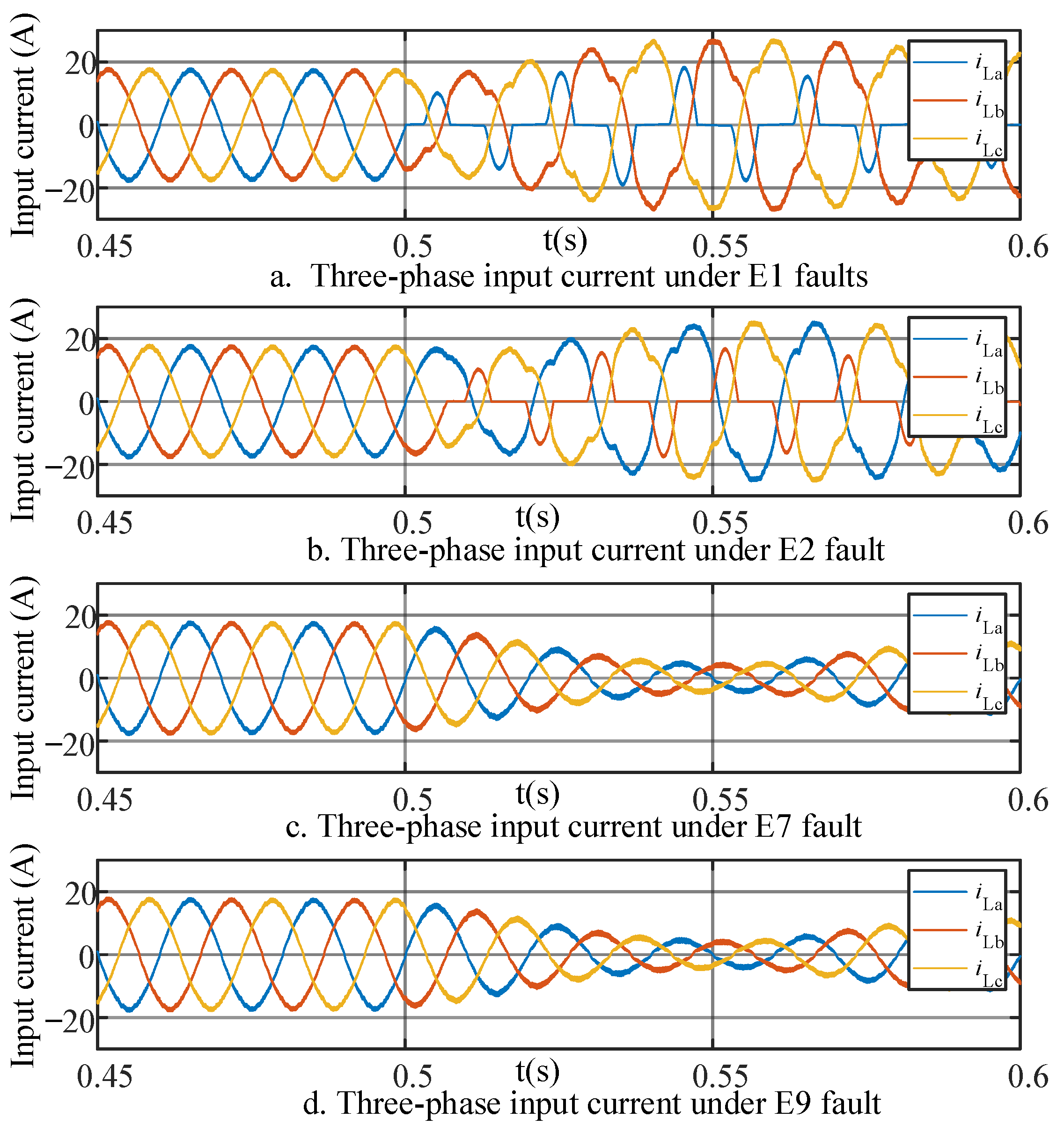
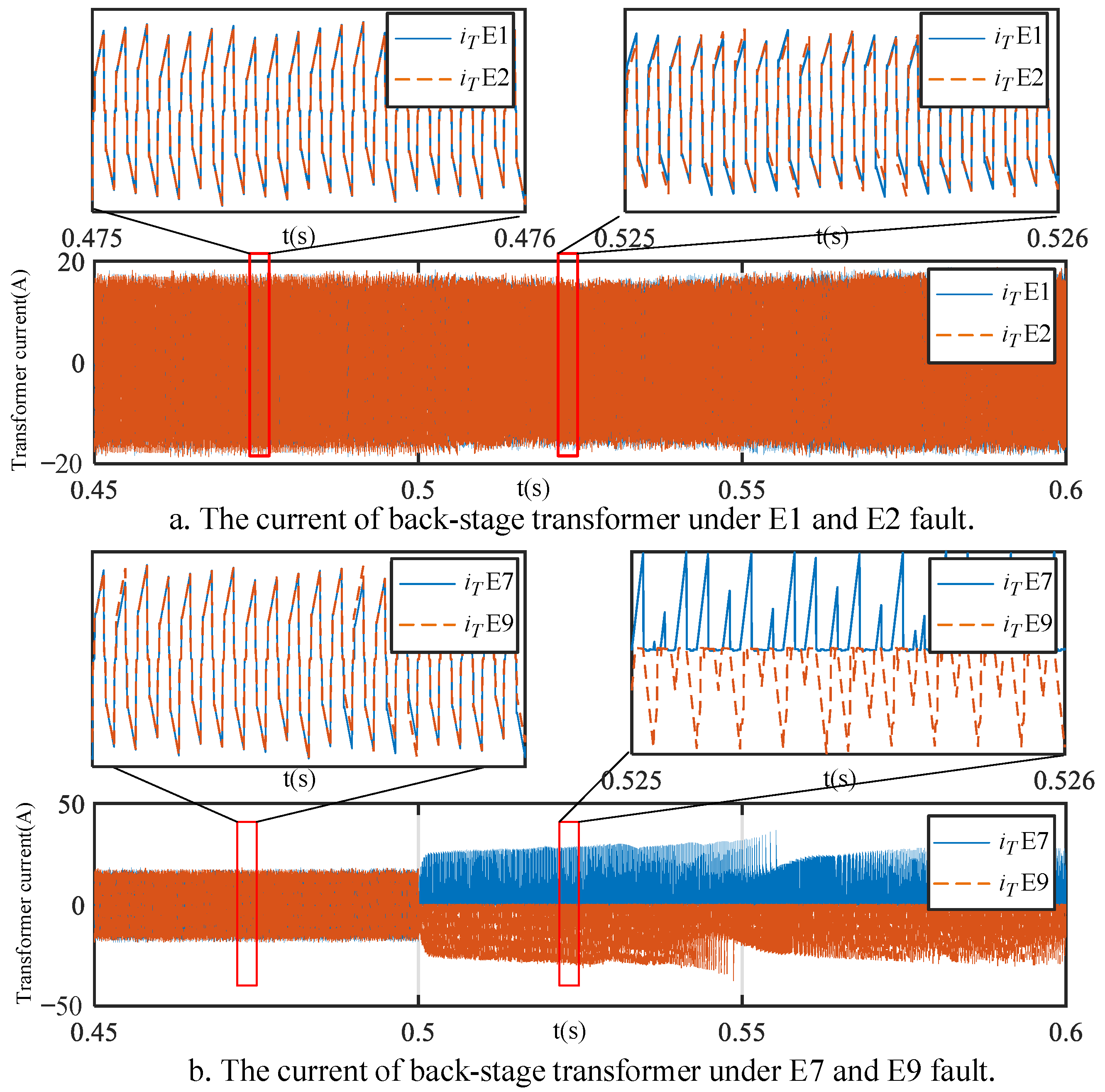
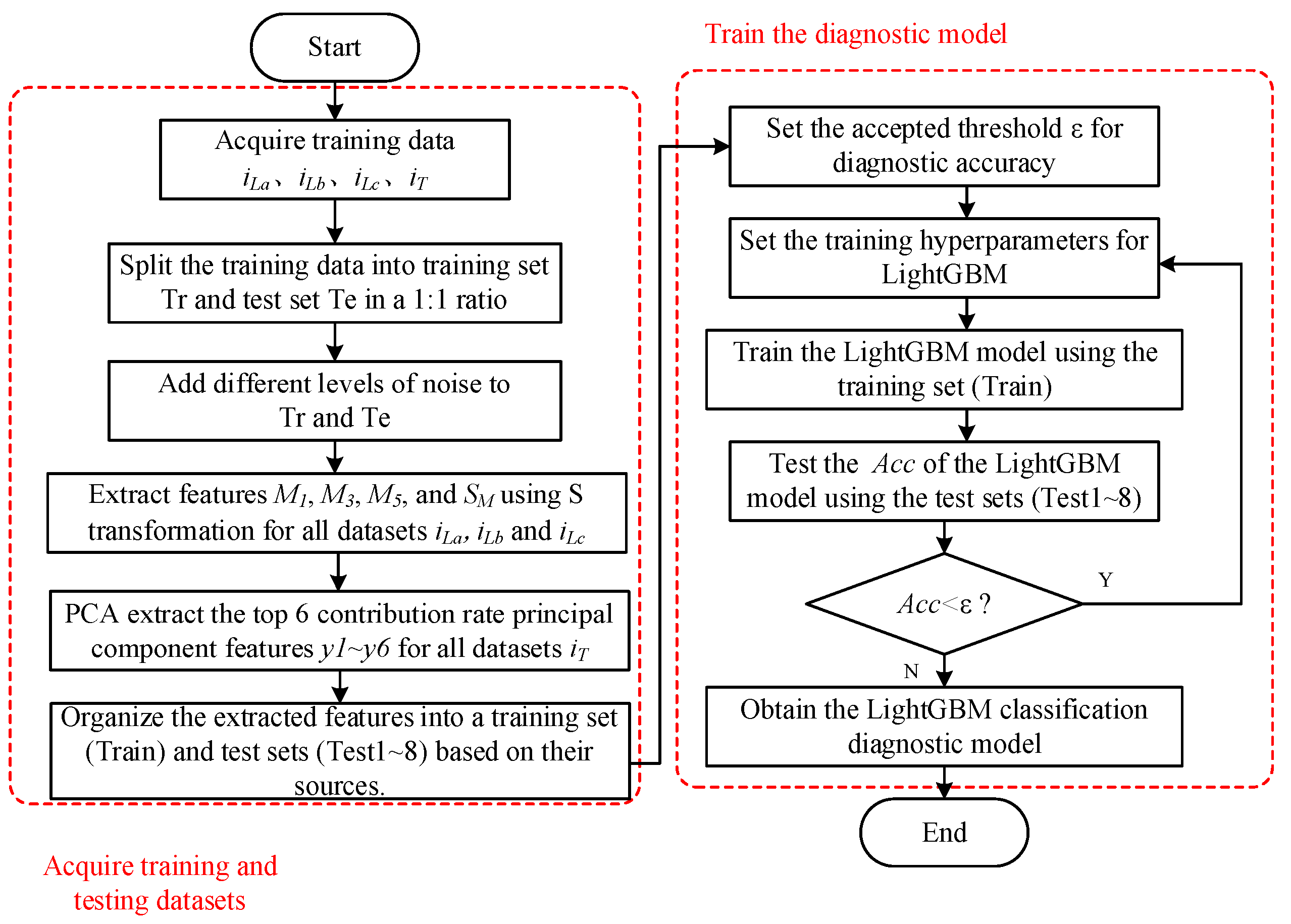
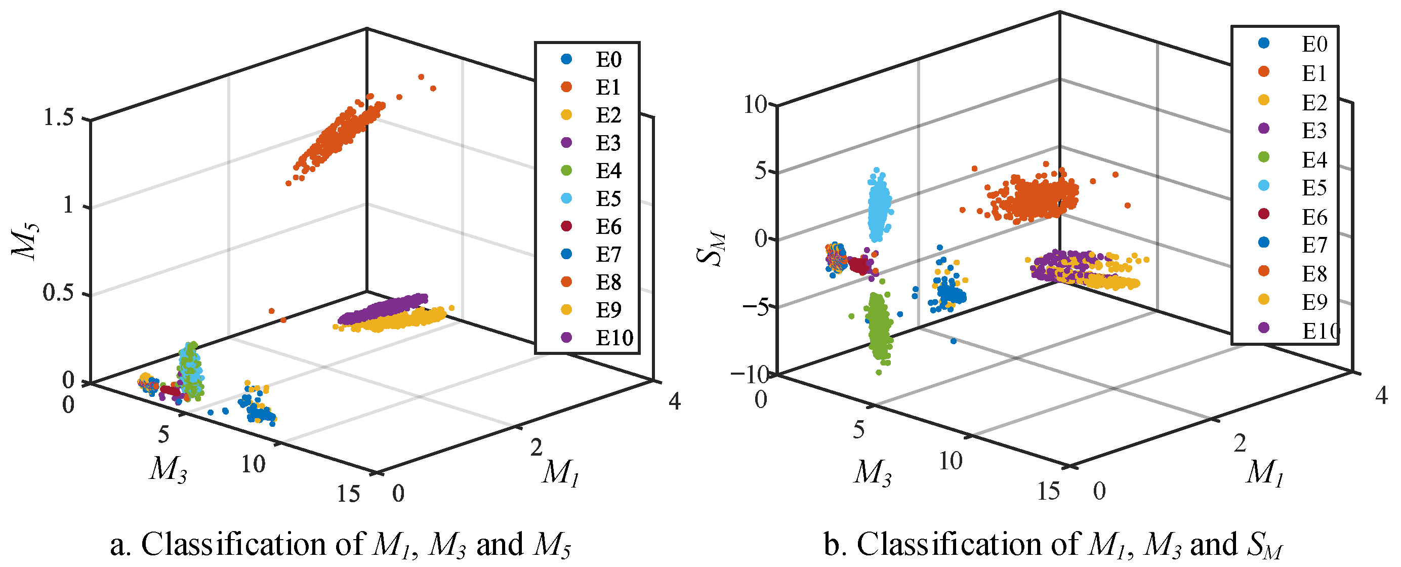
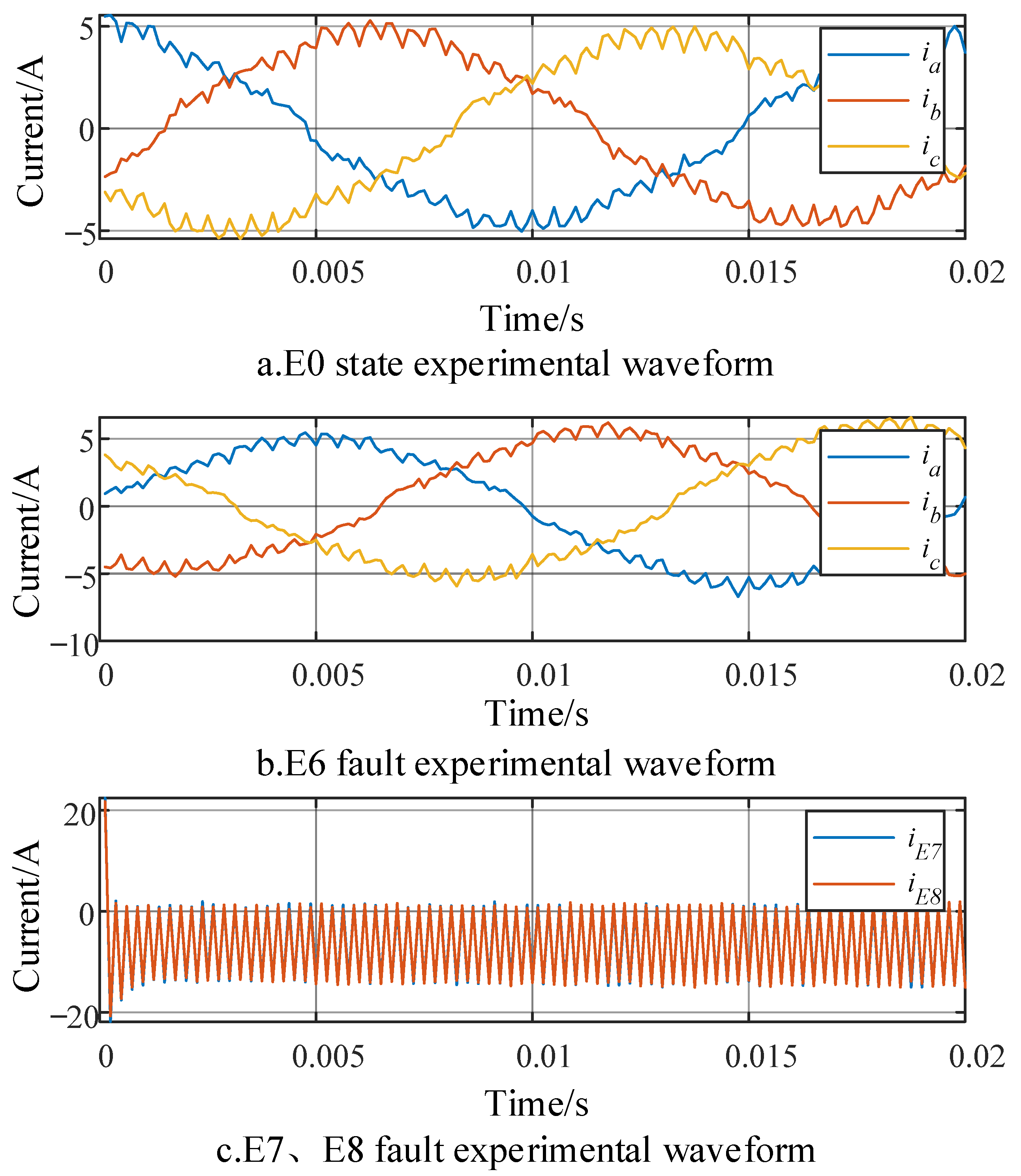
In this section, we’ll delve into the diagnostic methodology for electric vehicle DC charging pile openings, outlining a framework intricately woven with advancements in S-transform and LightGBM. First, we enhance the S-transform algorithm by tailoring it to the distinct characteristics of charging pile fault signals. The optimization process focuses on refining the window width, addressing incompleteness for an optimal outcome. Subsequently, we employ LightGBM to adeptly classify and extract features, culminating in a robust system for diagnosing charging pile failures.

3.1. Feature Extraction of Preliminary Faults Based on Improved S-Transform

S-transform is a proposed signal time-frequency analysis method. The principle involves a one-dimensional signal x(t), undergoing windowing operations and Fourier transformation to obtain a two-dimensional matrix ST(τ, f). The formula is as follows:

$$ST(\tau ,f)={\displaystyle \underset{-\infty }{\overset{\infty }{\int }}x(t)w(\tau -t,f)}{\mathrm{e}}^{-\mathrm{i}2\mathsf{\pi }ft}\mathrm{d}t$$

(1)

where w(τ − t, f) is the window function. The traditional S-transform uses the Gaussian window function. The expression is as follows:

$$w(\tau -t,f)=\frac{1}{\sigma \sqrt{2\mathsf{\pi }}}{\mathrm{e}}^{-\frac{{(\tau -t)}^2}{2{\sigma }^2(f)}}$$

(2)

where τ represents the central position of the window, and the variation of τ controls the sliding of the window along the time axis. σ(f) denotes the standard deviation of the Gaussian function and simultaneously serves as the window function adjustment factor.

In the realm of traditional S-transform, its limited control over the Gaussian window function width impedes the attainment of ideal time-frequency resolution at both low and high frequencies, resulting in suboptimal recognition accuracy. To address this challenge, researchers have introduced an enhanced version of S-transform. By refining the window function expression, this modified S-transform achieves superior time-frequency resolution. An example of such improvement is evident in the adjusted formulation of σ(f), as depicted in the following equation.

$$\sigma (f)=\frac{a}{b|f{|}^c+d}$$

(3)

where a, b, c, and d are adjustment factors that can be customized based on the actual signal. The generalized S-transform with adjustable window width offers better time-frequency resolution. However, such methods often rely on empirically enhanced window function expressions without clear theoretical foundations. Moreover, parameter tuning is intricate, and these approaches may not perform optimally when faced with changes in parameters such as sampling frequency. Hence, this paper introduces an incomplete S-transform algorithm based on effective window width improvement.

The two-dimensional matrix obtained through traditional S-transform encompasses temporal information for various frequency points. However, a substantial portion of these frequency point details constitute redundant values that are unnecessary for transformation. Hence, the principle of the incomplete S-transform is as follows:

S-transformation expression (1) can be transformed to the following expression:

$$ST(\tau ,f)={\displaystyle \underset{-\infty }{\overset{\infty }{\int }}U(\alpha +f)W(\sigma ,f){\mathrm{e}}^{\mathrm{i}2\mathsf{\pi }\alpha \tau }\mathrm{d}\alpha }$$

(4)

where U(α) represents the Fourier transform result of the signal x(t). Equation (4) indicates that the Fourier transform results U and W of the signal and the window function, respectively, can be used to transform specific frequency points f, yielding the temporal information for that frequency point. When the transformation is applied only to certain frequency points within U(α), it is referred to as incomplete S-transform. When analyzing fault characteristics, one can initially employ complete S-transformation. After selecting the characteristic frequency points, utilizing incomplete S-transform for signal processing eliminates a significant number of redundant calculations, thereby enhancing the real-time performance of the diagnostic algorithm.

Before performing the S-transform on specific frequency points, it is advisable to calculate the optimal window width for that frequency to achieve the best time-frequency resolution. The effective window width D for each frequency point with a Gaussian window function can be computed based on the frequency domain expansion σ_f and the 3σ energy coverage criterion of the window function. The process is outlined as follows:

$${\sigma }_f^2=\frac{{\displaystyle \sum _{-\infty }^{+\infty }{f}^2|W(\sigma ,f){|}^2\mathrm{d}f}}{{\displaystyle \sum _{-\infty }^{+\infty }|W(\sigma ,f){|}^2\mathrm{d}f}}=\frac{1}{8{\mathsf{\pi }}^2{\sigma }^2}$$

(5)

$${\sigma }_f^{}=\frac{1}{2\sqrt{2}\mathsf{\pi }\sigma }$$

(6)

In accordance with the 3σ criterion, the effective window width D is defined as the length of the horizontal axis interval covering 99.73% of the window function’s area. When $f=x{\sigma }_f$, the Gaussian window function is as follows:

$$W={\mathrm{e}}^{-x^2/4}$$

(7)

According to the normal curve nature, the horizontal axis interval $[-3\sqrt{2},3\sqrt{2}]$ contains the area of 99.73% of the Gaussian window function shown in Formula (7), so the Gaussian window function effective window width D is:

$$D=6\sqrt{2}{\sigma }_f=\frac{3}{\mathsf{\pi }\sigma }$$

(8)

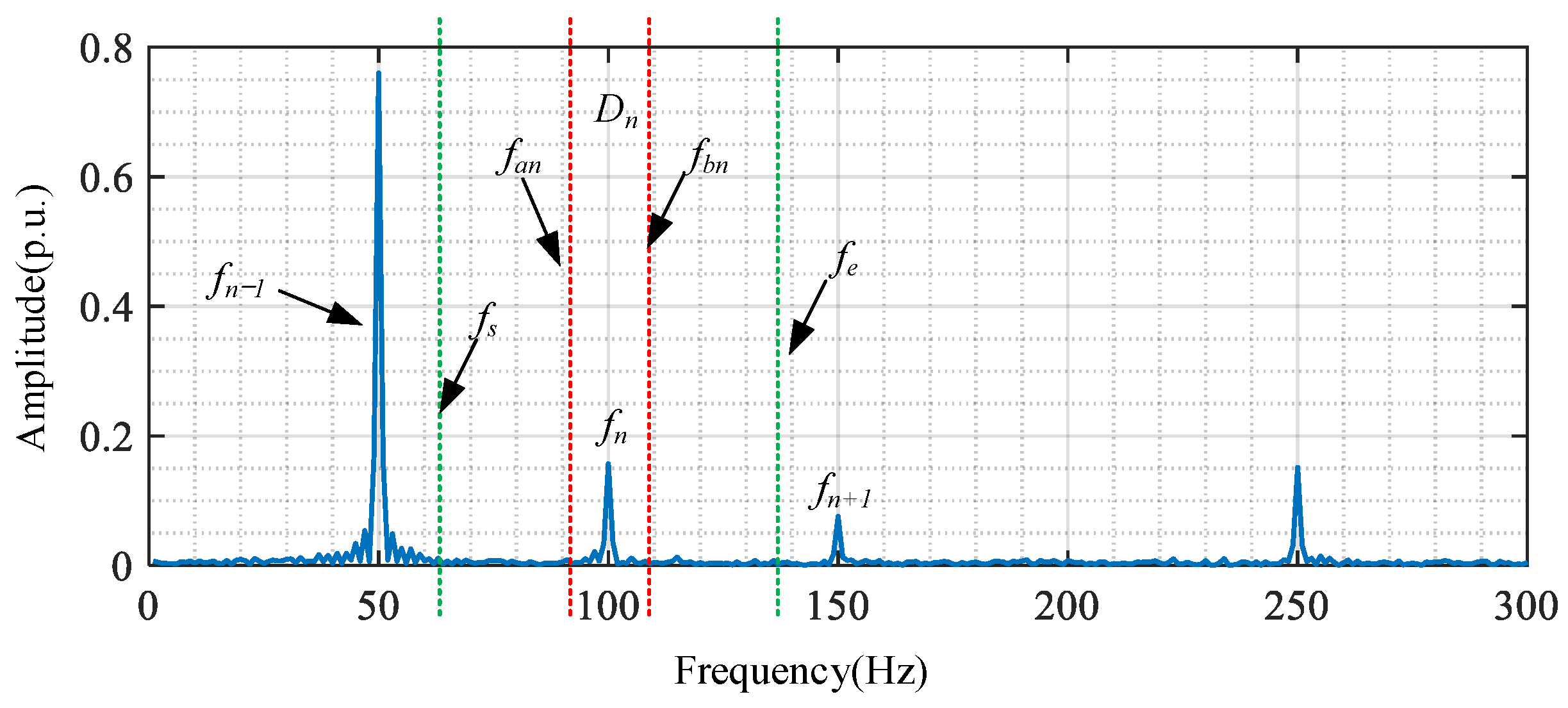
After performing the FFT transformation on the one-dimensional signal x(t), the spectrum U(f_k) is obtained. When the S-transform applies windowing to the spectrum, the effective window width D_n of the window function at the main frequency point f_n should cover the main value interval of f_n, as illustrated in Figure 4.

The main value interval corresponding to the main frequency point f_n can be calculated using the frequency point energy E_n, as follows:

$$E_n={\displaystyle \sum _{k=f_s}^{fe}|U(f_k){|}^2}$$

(9)

where f_s and f_e represent three-fourths between the main frequency point f_n and the preceding main frequency point f_n−1, and the succeeding main frequency point f_n+1. This can be expressed as follows:

$$\{\begin{array}{l}{f}_s=\frac{f_n+3f_{n-1}}{4}\\ f_e=\frac{3f_{n+1}+f_n}{4}\end{array}$$

(10)

Taking into account noise interference, when the energy E_D within the interval [f_an, f_bn] covered by the effective window width D_n accounts for 95% or more of E_n, it can be considered that the Gaussian window corresponding to this σ value has covered the main value interval of the frequency point f_n. The expression is as follows:

$$\frac{E_D}{E_n}=\frac{{\displaystyle \sum _{k=f_{an}}^{f_{bn}}|U(f_k){|}^2}}{E_n}\ge 95\%$$

(11)

With the interval [f_an, f_bn] being symmetric about the f_n axis, obtaining [f_an, f_bn], the calculation for σ is as follows:

$$\sigma =\frac{3}{\pi (f_{bn}-f_{an})}$$

(12)

In summary, this method calculates the optimal window width corresponding to each frequency point’s σ value through the effective window width D of the Gaussian window and the energy distribution characteristics of the test signal. It enables the selection of the optimal window width for each frequency point in the test signal, thereby conducting the S-transform. This approach mitigates issues arising from excessively narrow window widths, such as low-frequency domain resolution problems, or overly broad window widths leading to frequency aliasing and low time-domain resolution problems. The resulting improved S-transform achieves commendable time-frequency resolution.

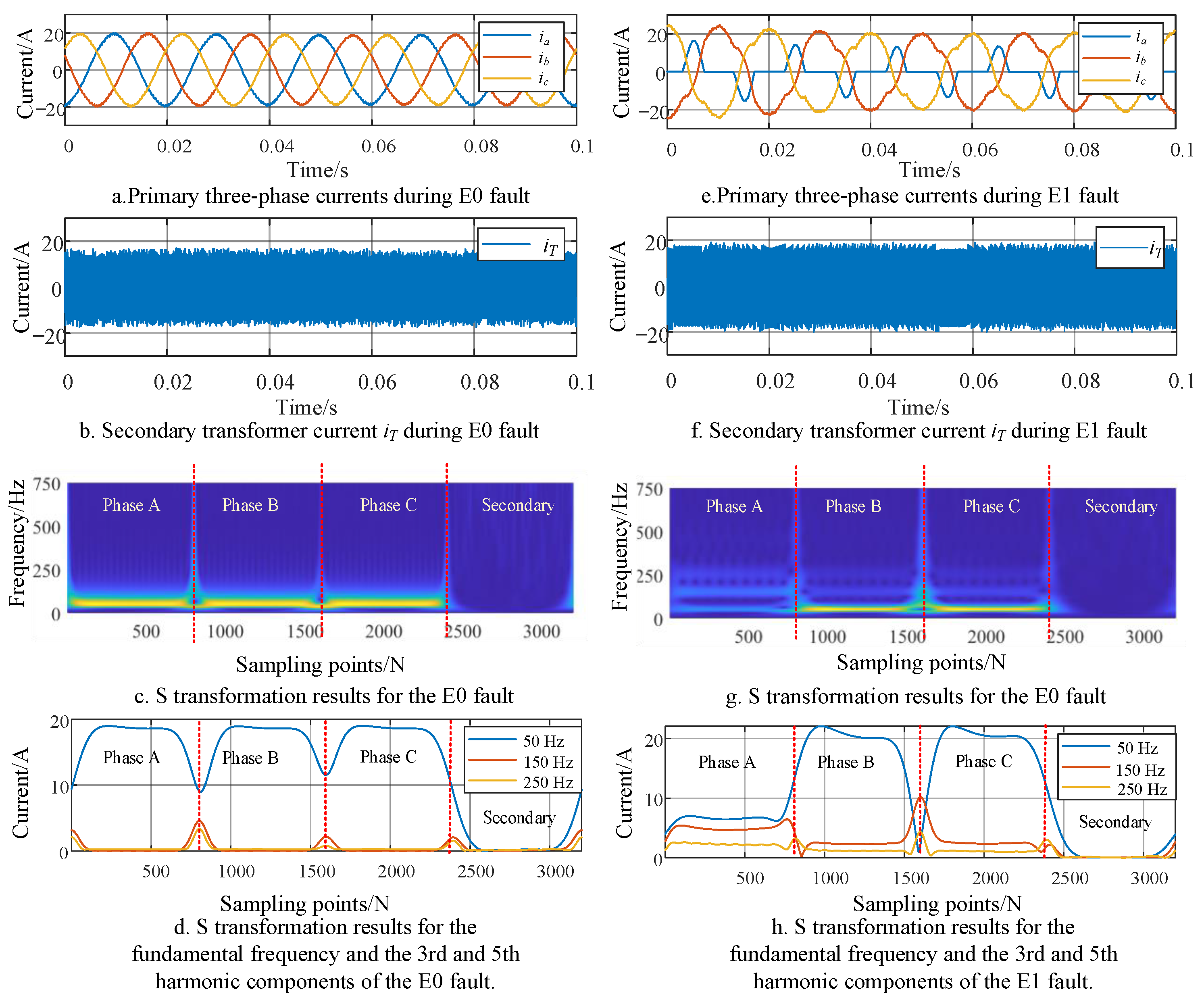
Based on the analysis in the previous section, the signal used for identifying primary faults is the three-phase sinusoidal waveform of the power frequency, suitable for feature extraction using the improved S-transform. The collected signal results with the improved S-transform for faults E0 and E1 are shown in Figure 5. In this case, the fused data x processed by the improved S-transform are formed by concatenating the three-phase currents (i_a, i_b, i_c) of the primary inductance A, B, and C, and the high-frequency transformer current i_T of the secondary stage. The data processing is described by the following equation:

$$x=[\begin{array}{cccc}{i}_a& i_b& i_c& i_T\end{array}]$$

(13)

Therefore, the results of the complete S-transform in Figure 5c,g can be divided into four parts based on the sampling points. These parts represent the complete S-transform results of the primary inductance currents i_a, i_b, and i_c for phases A, B, and C, and the high-frequency transformer current i_T of the secondary stage. Figure 5d,h depicts the improved incomplete S-transform results for the fundamental frequency and the 3rd and 5th harmonic components of the E0 and E1 fault data, respectively.

From the complete S-transform results in Figure 5, specifically c and g, it can be observed that after the occurrence of the E1 fault, the fundamental frequency amplitude of phase A decreases. Additionally, the waveforms of the three-phase currents A, B, and C contain 3rd and 5th harmonic components. However, the S-transform results of the secondary transformer current do not show a clear distinction within 700 Hz. As shown in Figure 5, specifically d and h, during the E1 fault occurrence, compared with phases B and C, the fundamental frequency amplitude of phase A is lower, the amplitude of the 3rd harmonic is higher, and the amplitude of the 5th harmonic is slightly higher.

Due to the three-phase symmetry of faults E2 and E3 with E1, fault characteristics for the primary faults E1, E2, and E3 can be extracted based on the results of the improved incomplete S-transform. The designated feature values for primary faults are set as follows.

The average values of the fundamental frequency in the incomplete S-transform results within each interval:

$$M_1=\frac{{\displaystyle \sum _{k=1}^{N}ST(k,50)}}{N}$$

(14)

where N represents the number of sampled data points for each phase.

The average values of the 3rd and 5th harmonic incomplete S-transform results within each interval are expressed as the following equations:

$$M_3=\frac{{\displaystyle \sum _{k=1}^{N}ST(k,150)}}{N}$$

(15)

$$M_5=\frac{{\displaystyle \sum _{k=1}^{N}ST(k,250)}}{N}$$

(16)

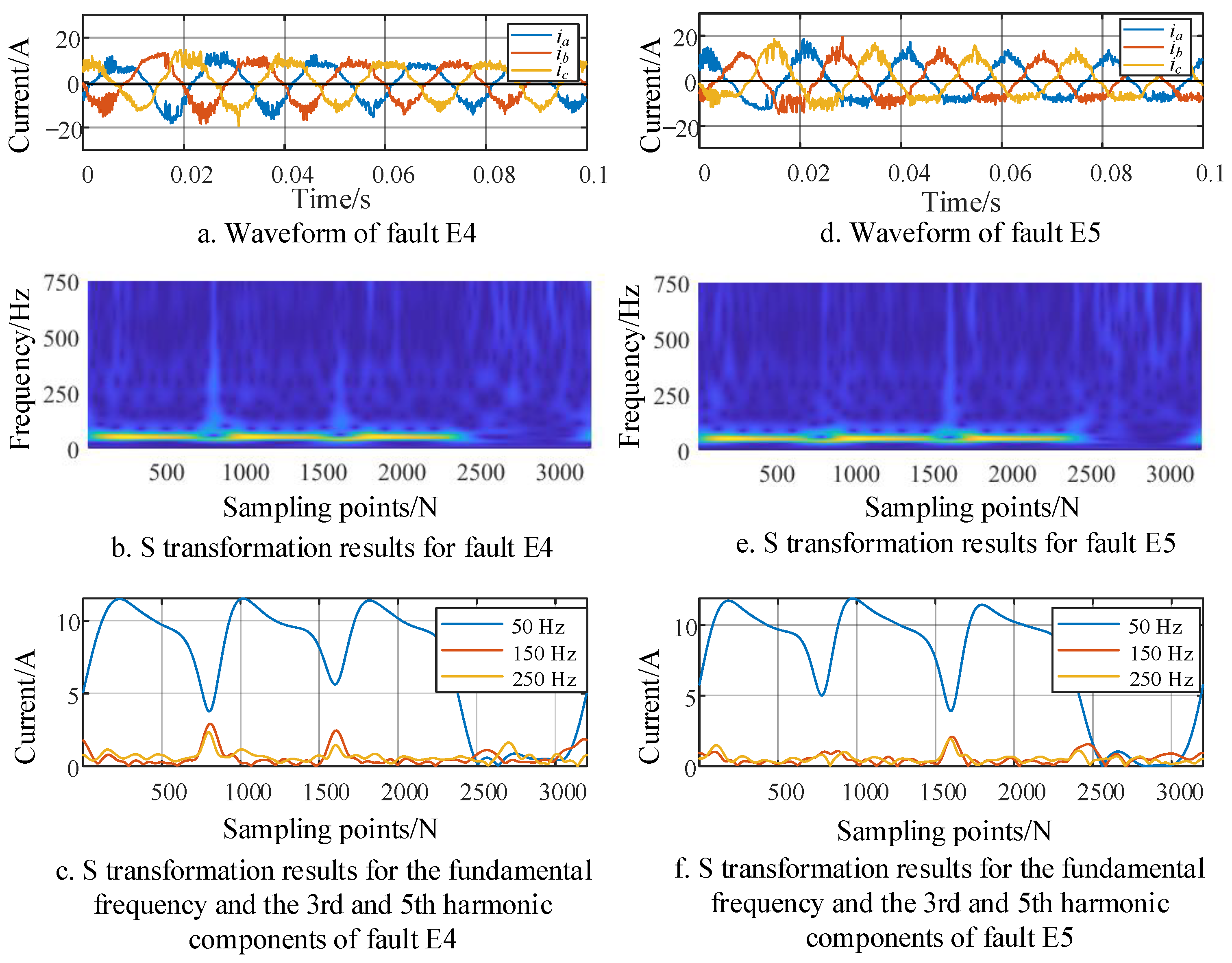
For the imbalance capacitor faults E4 and E5 in the VIENNA rectifier front stage, the fault waveforms and S-transform results are illustrated in Figure 6.

From the complete S-transform results in Figure 6, it can be observed that for faults E4 and E5, there is no distinct feature differentiation in the S-transform results. However, as shown in Figure 6a,d, due to the fault occurring at the balancing capacitor of the primary rectifier, causing the output voltage of the converter to be 0 during either the positive or negative half-cycle, the three-phase input currents will be clamped at a fixed value with a 120° phase difference during the positive and negative half-cycles due to the influence of inductance and other factors after the capacitor fault occurs. Based on this, specific feature values can be determined as follows, with the sum of the maximum and minimum values of the primary input current denoted as S_M:

$$S_M=\max (x)+\min (x)$$

(17)

3.2. Feature Extraction for Back-Stage Faults Based on PCA

PCA is a data dimensionality reduction method based on the concept of maximizing separability. It achieves this by linearly projecting data from high-dimensional space to a lower-dimensional one, generating principal component data. The principal component data encapsulates the primary features of the original data while eliminating certain inherent correlations. The process of extracting principal components in this data dimensionality reduction primarily relies on the theory of maximizing variance, as outlined below.

Assume that there are N groups of data ${[\begin{array}{cccc}{x}_1& x_2& \cdots & x_N\end{array}]}^T$ to be processed, and the length of each group of data is p, then there is a sample matrix X.

$$X=\left[\begin{array}{cccc}{x}_{11}& x_{12}& \cdots & x_{1p}\\ x_{21}& x_{22}& \cdots & x_{2p}\\ ⋮& ⋮& \ddots & ⋮\\ x_{N1}& x_{N2}& \cdots & x_{Np}\end{array}\right]$$

(18)

Calculate the covariance matrix C of the sample matrix X and obtain the correlation coefficient between each sample.

$$C=\left[\begin{array}{cccc}c(x_1,x_1)& c(x_1,x_2)& \cdots & c(x_1,x_N)\\ c(x_2,x_1)& c(x_2,x_2)& \cdots & c(x_2,x_N)\\ ⋮& ⋮& \ddots & ⋮\\ c(x_N,x_1)& c(x_N,x_2)& \cdots & c(x_N,x_N)\end{array}\right]$$

(19)

$$c(x_m,x_k)=\frac{1}{N-1}{\displaystyle \sum _{i=1}^N(x_{mi}-\overline{x_m})(x_{ki}-\overline{x_k})}$$

(20)

Then, perform eigenvalue decomposition on the covariance matrix C to obtain its eigenvalue λ and eigenvector w.

$$Cw=\lambda w$$

(21)

The eigenvalues of the covariance matrix represent the contribution of each principal component. The ordering of them is as follows: ${\lambda }_1\ge {\lambda }_2\ge \cdots \ge {\lambda }_N$. The eigenvectors corresponding to the largest d eigenvalues can be taken to form a reduced-dimensional projection matrix $W=[\begin{array}{cccc}{w}_1& w_2& \cdots & w_d\end{array}]$. The process of reducing the sample matrix X from N dimensions to d dimensions through principal component analysis is as follows.

$$Y=XW$$

(22)

Finally, a d-dimensional sample matrix Y is obtained, and the contribution rate r_i of each principal component is:

$$r_i=\frac{{\lambda }_i}{{\displaystyle \sum _{k=i}^p{\lambda }_k}}$$

(23)

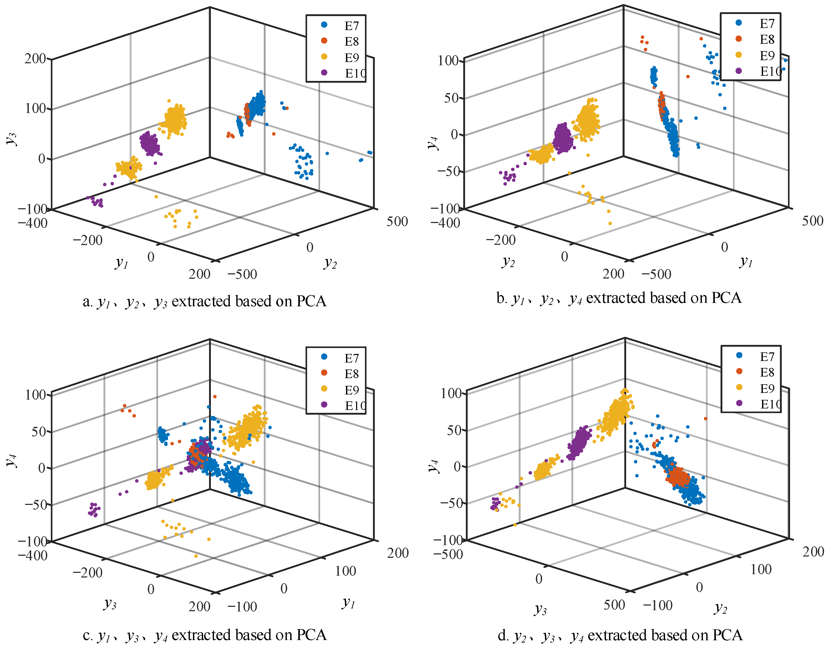
Perform PCA processing on the collected downstream transformer current i_T data. The processed data are set to be i_T data 0.02s after the fault. The data length is 160 points. The top 10 contribution rates of the extracted principal components are shown in the

Table 2. Contribution rates of the principal components extracted through PCA for the secondary stage.

Feature	y1	y2	y3	y4	y5	y6	y7	y8	y9	y10
Contribution rate	0.6937	0.1416	0.0100	0.0041	0.0041	0.0011	0.0009	0.0008	0.0007	0.0007

.

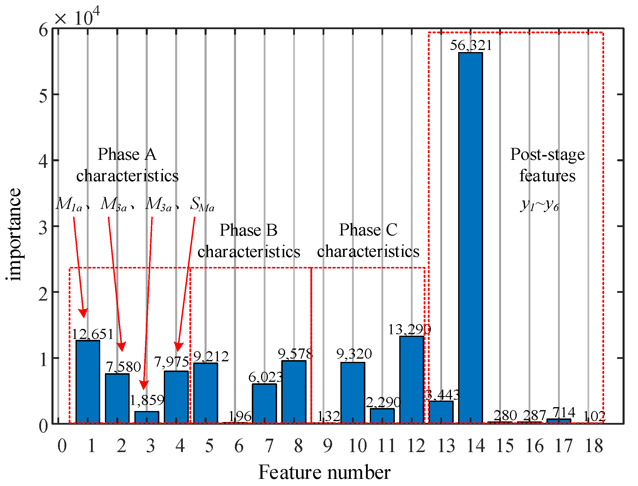
As can be seen in Table 2, the contribution rate of the top 10 features accounted for 85.62%, and the contribution rate of the top six principal components accounted for 85.32%. Therefore, the first six principal components with contribution rates are selected as the subsequent stage fault characteristic values.

3.3. Feature Classification Diagnosis Based on LightGBM

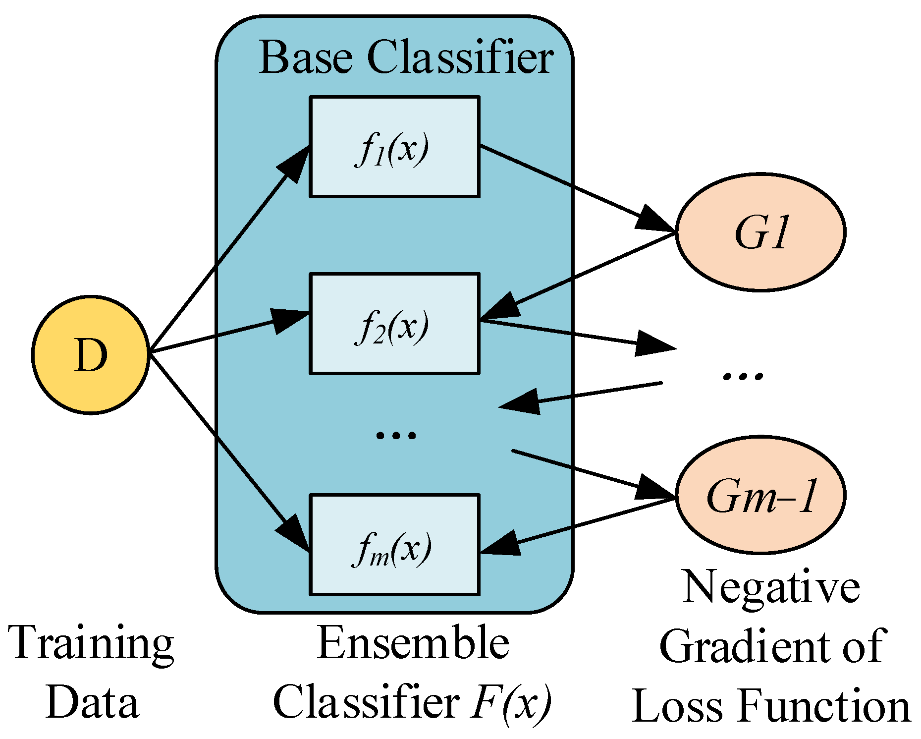
The LightGBM algorithm is an ensemble learning model based on a decision tree (DT), with the DT serving as its foundational classifier model. LightGBM utilizes gradient boosting technology. Boosting is an ensemble learning algorithm that involves linearly combining multiple sequentially generated base classifiers to integrate training and obtain a more powerful model. Its framework can be described as follows:

$$F(x)={\displaystyle \sum _{i=1}^m{\alpha }_i{f}_i(x)}$$

(24)

where F(x) represents the ensemble classification model obtained through training, m denotes the number of base classifiers f_i(x), and α_i represents the weight of the base classifier.

Each time a new base classifier is generated, gradient boosting follows the direction of gradient descent based on the loss function of the previous base classifier. Assuming the loss function of the ensemble classification model is L(F(x), y) for gradient boosting, the framework would be as follows:

$$F_i(x)=F_{i-1}(x)-{\alpha }_i\frac{\partial L(F_{i-1}(x),y)}{\partial F_{i-1}(x)}$$

(25)

$$f_i(x)\approx -\frac{\partial L(F_{i-1}(x),y)}{\partial F_{i-1}(x)}$$

(26)

In other words, each newly generated base classifier f_i(x) fits the negative gradient of the loss function of the previous ensemble classifier F_i−1(x). Through continuous iterations, the ensemble classifier F(x) systematically reduces errors, ultimately resulting in a classifier with higher accuracy. Its fundamental principle is depicted in Figure 7.

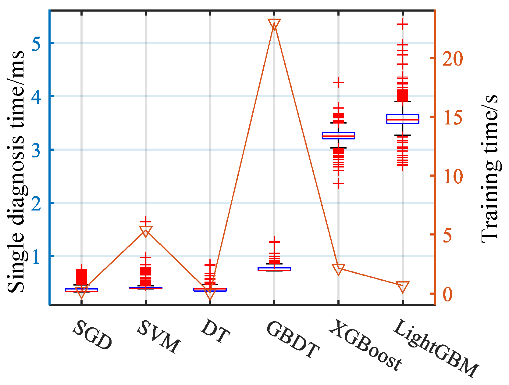
LightGBM is a lightweight gradient boosting model developed to cater to the needs of handling massive datasets, building upon the foundation of XGBoost. Addressing the challenges posed by XGBoost, such as high memory requirements and computational time, LightGBM optimizes various aspects. This includes reducing the computational load of splitting points, minimizing the quantity of training data, managing the number of feature values, and optimizing decision tree construction strategies.

With these enhancements and optimizations, LightGBM achieves faster data processing speed and lower memory usage without compromising accuracy. It demonstrates the capability to swiftly handle massive datasets.

3.4. LightGBM Diagnosis Model and Process

Based on the aforementioned content, this section employs the LightGBM diagnosis model to diagnose open-circuit faults in electric vehicle DC charging piles. The overall process of obtaining the diagnosis model is illustrated in Figure 8.

As illustrated in the flowchart, the original dataset undergoes S-transforms such as the improved S-transform and PCA to generate a feature dataset. The training section of the LightGBM diagnostic model utilizes this feature dataset for training and testing adjustments, enabling the diagnostic model to develop the ability to diagnose faults based on features.

During the diagnosis process, this diagnostic model employs improved S-transform and PCA algorithms to extract fault features from the fault signals i_a, i_b, i_c, and i_T in the charging module circuit of the electric vehicle charging pile. Subsequently, the LightGBM algorithm is used to recognize and diagnose the extracted fault features.

4. Simulation and Experimental Analysis

In this section, the dataset is established through the Simulink simulation model, the diagnostic model is trained and tested by Python, and finally, a charging module fault diagnosis experimental platform is built based on RT-Lab to experimentally verify the diagnostic model. The software/hardware environment used for simulation verification is shown in

Table 3. Simulation test environment.

Software/Hardware	Model/Version	Software/Hardware	Model/Version
OS	Win10 64 bit	RAM	DDR4 8 GB
CPU	i5 9300H	HDD	SSD 500 GB
GPU	GTX 1650 4 GB	Python	3.6

.

4.1. Create the Dataset

A simulation model was built based on the charging module circuit topology in Section 2.1. The circuit design parameters are shown in

Table 4. Table of circuit parameters.

Parameters	Value
Three-phase line voltage of front stage	380 V ± 5%
Output voltage of front-stage VIENNA rectifier	750 V ± 10%
Switching frequency of front-stage VIENNA rectifier	50 kHz
Output voltage of back-stage phase-shifted full-bridge converter	375 V ± 5%
Switching frequency of back-stage phase-shifted full-bridge converter	20 kHz
Rated output power of charging module	15 kW
Front-stage inductor	1.5 mH
Flat capacitor of front-stage VIENNA rectifier	3 mF
Inductor of back-stage output filter	100 µH
Capacitor of back-stage output filter	100 µF
Load resistance of back stage	20 Ω

.

During each simulation, the capacitance component parameters in the circuit fluctuate by ±20%, the inductance parameters fluctuate by ±10%, the load fluctuation range is 10~200%, and the set fault occurs randomly within 0.1~0.2 s after reaching the steady state. The operating data are collected within 0.2 s after the fault occurs. The signal sampling frequency is 8 kHz, and a total of 4 × 1600 data of i_a, i_b, i_c, and i_T are collected each time. Each fault type is simulated 1000 times, and a total of 11,000 sets of noise-free fault data are generated to form the dataset.

Since LightGBM can obtain good diagnostic results using a small amount of data training, this article randomly intercepts 1/5 of the data of each fault type in the dataset, and intercepts the data 0.02 s after the fault occurs. Each set of data is 4 × 160 points long. Finally, the dataset D_o is obtained.

The feature dataset D_o is divided into a noise-free training set Tr and a noise-free test set Te according to 1:1. Different levels of noise are added to Tr and Te to obtain the signal dataset, as shown in

Table 5. Fault signal dataset composition.

Dataset	SNR/dB	Dataset	SNR/dB
Tr_0	noise-free	Te_2	15
Tr_1	15	Te_3	20
Tr_2	20	Te_4	25
Tr_3	30	Te_5	30
Te_0	noise-free	Te_6	35
Te_1	10	Te_7	40

.

The improved S transform is used to extract the front-stage features M₁, M₃, M₅, and S_M from the data in the signal dataset Tr_0. In order to reflect the characteristics of four-dimensional data, Figure 9a shows the scatterplot of M₁, M₃, and M₅ feature spaces, and Figure 9b shows the scatterplot of M₁, M₃, and S_M feature spaces.

From Figure 9a, we can see that E0, E1, E2, E3, and E6 have good separation from other faults in the M₁, M₃, and M₅ feature spaces, but E4, E5, and E7~E10 E4, E5 and E7~E10 have poor separation in the feature space. From Figure 9b, we can see that E0, E1, E4, E5, and E6 all have good separation in the feature spaces of M₁, M₃, and S_M, but back-stage faults E7~E10 have poor separation in the feature space. Fault types with good separation in the feature space are easier to classify. Therefore, the features M₁, M₃, M₅, and S_M extracted based on the improved S transform can differentiate and diagnose faults E0~E5 and fault E6.

As shown in the Figure 8, the improved S-transform is used to extract the features M₁, M₃, M₅, and S_M of all signal datasets i_a, i_b, and i_c in Table 5 to form the feature datasets P_tr and P_te.

The high-frequency transformer current i_T data of the downstream circuit in the signal dataset Tr_0 are processed by PCA, and the extracted principal components y₁~y₄ are drawn into a feature space scatter diagram, as shown in Figure 10. As can be seen in Figure 10, the back-stage faults E7, E8, E9, and E10 have good separation in the feature spaces of Figure 10a,b,d. There is also a certain degree of separation between E7 and E8, and E9 and E10. Therefore, selecting the top six features y₁~y₆ in the contribution rate of the principal component analysis results as the back-stage features can identify the back-stage faults E7~E10.

As shown in the Figure 8, PCA is used to extract the top six principal component features y₁~y₆ of iT contribution rate in all signal datasets in

Table 6. Simulation test environment.

Dataset	Feature Set	Original Signal Set	Dataset	Feature Set	Original Signal Set
Train	Ptr0, Btr0	Tr_0	Test_3	Pte2, Bte2	Te_2
	Ptr1, Btr1	Tr_1	Test_4	Pte3, Bte3	Te_3
	Ptr2, Btr2	Tr_2	Test_5	Pte4, Bte4	Te_4
	Ptr3, Btr3	Tr_3	Test_6	Pte5, Bte5	Te_5
Test_1	Pte0, Bte0	Te_0	Test_7	Pte6, Bte6	Te_6
Test_2	Pte1, Bte1	Te_1	Test_8	Pte7, Bte7	Te_7

to form the feature datasets B_tr and B_te.

The training set Train and test set Test 1~8 of the diagnostic model are combined with the extracted front and back stages feature datasets, as shown in the table below.

4.2. Fault Diagnosis Model Training

The LightGBM diagnostic model training flowchart in Section 3.4 is followed to train the diagnostic model. The initial parameters are set as: N = 5, N_br = 3000, L_r = 0.01, ES = 5, and the parameters N_le and M_dl are optimized. The N_le value range [2, 100] is set with a step size of 1, and the M_dl value range [100, 1010] with a step size of 100, and the training parameters of the model are optimized.

Diagnostic accuracy Acc is used to evaluate model performance, and its expression is:

$$Acc=\frac{1}{m}{\displaystyle \sum _{i=1}^{N}T{P}_i}$$

(27)

In the formula, m represents the number of all samples, N represents the number of sample types, and TP_i represents the number of correct diagnoses in the i-th type of samples.

The relationship between model Acc and N_le and M_dl parameters is obtained as shown in Figure 11.

As can be seen in Figure 11, when the values of N_le and M_dl are small, the change of model diagnosis accuracy Acc is related to the two values. When N_le is greater than 40 and M_dl is greater than 200, Acc and the value are only related to the change of M_dl. This shows that when the M_dl number of LightGBM is constant, N_le is set to a larger value. In the actual model, the number of decision tree leaves will also be maintained at a relatively small optimal value through training and optimization. When N_le is constant, the model diagnostic performance is related to the M_dl setting. Taking the minimum N_le value and M_dl value when Acc is the highest in the Figure 11 as training parameters, and their values are 25 and 400, respectively.

After selecting the parameters, the training data are used to train the model, and the importance score of each feature for classification is obtained, as shown in Figure 12 below. The feature importance score reflects the contribution of the feature to the classification gain during classification, and is calculated using the Gini coefficient in LightGBM. It can be seen that each feature value extracted through S-transform and PCA plays a certain role in classification. Among them, the subsequent feature y2 extracted through PCA makes the greatest contribution to classification.

The change results of the multi-classification loss value of the training set are as follows.

As can be seen in Figure 13, the classification loss of LightGBM continues to decrease during training, until ES is triggered to converge at 437 generations, and the model training is completed.

4.3. Diagnostic Model Comparison Test

In order to further test the effectiveness, noise resistance, generalization ability, and real-time performance of the algorithm proposed in this section, this section compares the trained diagnostic model with the traditional diagnostic model. The diagnostic algorithms compared include stochastic gradient descent (SGD), SVM, DT, GBDT, and XGBoost.

All algorithms are trained using the training set Train obtained before. The anti-noise test set Test 1~8 is used for accuracy testing. The test results are shown in

Table 7. Comparison of diagnostic algorithm noise immunity test results.

Algorithm	Accuracy/%
	10 dB	15 dB	20 dB	25 dB	30 dB	35 dB	40 dB	Noise-Free
SGD	70.90	71.18	72.64	71.54	71.09	71.63	72.45	72.18
SVM	86.36	92.00	92.00	93.18	93.18	93.27	93.18	93.63
DT	75.09	81.27	90.36	91.90	93.27	94.45	95.45	96.00
GBDT	92.45	96.54	97.45	97.45	98.18	97.72	97.72	97.45
XGBoost	90.00	96.72	97.00	97.90	98.18	98.27	98.09	98.27
LightGBM	90.81	97.18	97.18	97.90	98.18	98.27	98.36	98.45

.

The accuracy of each algorithm in diagnosing the features extracted by the method proposed is above 70%, in Table 7, with the highest diagnostic accuracy reaching 98.45%. This indicates that the features extracted by the method proposed in this paper can achieve fault diagnosis for electric vehicle charging stations.

The training set and verification set used by the diagnostic algorithm only contain 15 dB, 20 dB, 30 dB, 40 dB, and noise-free data. The diagnostic accuracy of each algorithm in the 10 dB, 25 dB, and 35 dB test set is not significantly lower than other results, which means that the algorithms tested and compared all have certain generalization capabilities. In Table 7, The accuracy of each algorithm increases as the noise intensity in the test dataset decreases. Compared with other decision tree-related algorithms, SGD and SVM have overall lower diagnostic accuracy and poorer diagnostic performance, which shows that the decision tree related algorithm is more suitable for classifying and diagnosing the characteristics of electric vehicle charging piles. Among the decision tree-related algorithms, the diagnostic accuracy of DT drops by 14.73% when the SNR is 15 dB, and its noise immunity is poorer than other algorithms.

The diagnostic accuracy of the GBDT, XGBoost, and LightGBM algorithms in the noisy test set with SNR greater than 15 dB is no more than 2% different from the accuracy in the noise-free test set. Even in the case of high noise with SNR 10 dB, the three algorithms still have an accuracy of more than 90%. It shows good noise immunity. In particular, LightGBM has the highest diagnostic accuracy in the test set, with SNR greater than 25 dB.

The comparison content of the real-time comparison test is the training time and single diagnosis time of each algorithm. The algorithm’s single diagnosis time consumption is recorded as the diagnosis time of each group of data when the algorithm diagnoses 1000 groups of data. The training time is drawn as a line chart, and the 1000 groups of single diagnosis time is drawn as a box plot for comparison. The results are shown in Figure 14 below.

In Figure 14, it can be observed that the single-diagnosis time of the SGD, SVM, and DT algorithms is at a relatively low level, with an average single-diagnosis time of less than 0.5 ms. This is because these three algorithms have relatively simple principles and require lower computational effort for diagnosis. However, the simplicity of their algorithmic principles also leads to poorer performance in noise resistance testing.

Among the remaining three algorithms, LightGBM has the shortest training time due to lightweight improvements in reducing split point computation, optimizing decision tree construction strategies, reducing the amount of training data, and decreasing the number of feature values. It only takes 0.67 s to complete the training of the diagnostic model. The training times are 31.3% and 2.9% of the training times for XGBoost (2.14 s) and GBDT (22.96 s), respectively.

However, the leaf-wise growth strategy and histogram algorithm make LightGBM build deeper trees, resulting in longer single-diagnosis times compared with GBDT and XGBoost, which directly classify feature values. The diagnostic model proposed in this section requires only 0.67 s for training in the simulation platform’s software and hardware environment, and the single-signal processing and classification diagnosis time is only 3.91 ms. This indicates that the proposed method requires lower computational effort for training and diagnosis, making it suitable for deployment on low-cost and low-performance computing platforms on a large scale.

The average time consumption for each stage of single-fault diagnosis, considering 1000 instances of single-feature extraction time for front and back stages signals, combined with the single-diagnosis time and signal sampling time of LightGBM, is presented in

Table 8. The average time consumption for each stage of single-fault diagnosis.

Stage	Average Time Consumption/ms
Signal sampling	20
Front-stage feature extraction based on S-transform	0.27
Back-stage feature extraction based on PCA	0.049
LightGBM feature classification diagnosis	3.59
Total time for single diagnosis	23.91

.

From the results in Table 8, it can be observed that in a single diagnosis, the average time consumption for the feature extraction and classification diagnosis processes on the simulation platform is 3.91 ms. Moreover, the signal processing time is much lower than the signal sampling time, enabling real-time signal processing. The comparison of the single-diagnosis time of the proposed diagnostic method in this section with the diagnostic time data from literature on open-circuit fault diagnosis in some power electronic devices is shown in

Table 9. Real-time performance comparison of diagnostic methods.

Algorithm	Sampling Time/ms	Diagnostic Computation Time/ms	Total Time for Single Diagnosis/ms
MB	-	3.45–113	-
MVP	-	12–14	-
RVFL	20	22	42
WPT-LSTM	10	15–33	25–43
LSTM	166	16	182
1DCNN-LSTM	20	-	-
Proposed method	20	3.91	23.91

Note: “-” indicates that the data are not mentioned.

below.

From Table 9, the total time for single diagnosis of 23.91 ms is excellent for open-circuit fault diagnosis in power electronic devices, meeting the requirements for electric vehicle charging station fault diagnosis.

In summary, the proposed method for open-circuit fault diagnosis in electric vehicle DC charging stations based on S-transform and LightGBM is effective in extracting fault features and achieving accurate diagnosis. Its average diagnostic accuracy reaches up to 97.04%, the highest among the compared algorithms. The method demonstrates excellent generalization, noise resistance, and real-time performance.

4.4. Experimental Diagnostic Effect Verification

To further validate the effectiveness of the proposed fault diagnosis technology, this paper constructs a semi-physical simulation experimental platform, as shown in Figure 15.

RT-LAB consists primarily of an upper computer, communication module, power module, and OP5700 simulator. Among these, the OP5700 simulator stands as the core for real-time simulation. The simulator houses multiple I/O boards internally, supporting up to 128 channels of analog signals or 256 channels of digital signals for input and output. During RT-LAB operation, models are transmitted to the OP5700 simulator via the communication module. The OP5700 compiles the simulation model and initiates real-time simulation. Real-time signal interaction is accomplished through integrated I/O boards. Within the simulation platform, a signal acquisition card collects fault signals outputted in real time by RT-LAB. These signals are simultaneously transmitted to the signal diagnostic upper computer for diagnosis. The signal acquisition card utilized is the USB DAQ-7606I produced by AUMANYU. It supports synchronized sampling of eight channels of analog signals, bidirectional input functionality, and has a range of −10 V to +10 V, a 16-bit AD resolution, and a multi-channel continuous sampling speed of 100 Hz to 20 kHz. This meets the 8 kHz data sampling frequency requirements for the diagnostic method proposed in this paper. In this experimental platform, RT-LAB is capable of compiling and running power electronics simulation models built in Simulink. It can interact with external hardware circuits through the onboard IO card and FPGA, enabling semi-physical simulation. The platform can simulate fault scenarios in the charging module under different circuit parameters and test the fault diagnosis capability of the proposed diagnostic model.

During the experiment, RT-LAB simulates faults in the charging module and generates fault signals. These signals, including i_La, i_Lb, i_Lc, and i_T, are then collected by the signal acquisition card. The collected data are transmitted to the signal analysis host computer, where the host computer utilizes the trained diagnostic model for fault diagnosis.

The waveforms of faults E1 to E6 obtained under rated power conditions are shown in Figure 16. In the oscilloscope display, the upper half shows the waveforms of i_a, i_b, and i_c, while the lower half displays the waveform of i_T.

The oscilloscope current waveforms for the back-stage faults E7 to E10 obtained under rated power conditions are shown in Figure 17.

In Figure 17, it can be observed that under rated power conditions, the measured input current waveforms for front-stage faults and the input current waveforms for back-stage high-frequency transformer faults are generally consistent with the simulated current waveforms. This indicates that the experimental platform operates stably, and the collected experimental fault data can be used to test the diagnostic algorithms.

To adapt to the range of the data acquisition card, the current data output has been scaled down by a factor of 10. Therefore, the experimental fault data collected by the data acquisition card need to be amplified by a factor of 10 first. Then, based on the set data size of 160 for each type of fault and the sampling frequency of 8 kHz of the data acquisition card, fault data are extracted for 0.02 s after each type of fault occurs. Since there is no specific fault occurrence time in the normal state, data for 0.02 s before each type of fault occurrence are randomly selected as the normal state type. After processing the data for each type of fault, the final experimental dataset De is established.

For fault diagnosis, it is necessary to extract features from the fault data in De. Therefore, the improved S-transform and PCA are first used to extract the front-stage features P for all i_a, i_b, i_c data in the experimental fault dataset and the back-stage features B for all i_T data. The feature data P and B are then combined into the feature dataset T and input into LightGBM for diagnosis.

The confusion matrix obtained from diagnosing the experimental fault data using the diagnostic model is shown in Figure 18.

In Figure 18, it can be observed that the recall rates for diagnosing various faults are above 80%, with a recall rate of 100% for front-stage faults. The diagnostic model achieves an accuracy of 96.36% for the experimental data, slightly lower than the performance of 98.45% for the simulated noise-free test set. This discrepancy is speculated to be due to the smaller sample size in the experimental test dataset, leading to a greater impact of misdiagnosis. In Figure 18, the diagnostic algorithm primarily exhibits diagnostic errors for back-stage faults. Some fault experimental waveforms collected by the acquisition card, along with the misdiagnosed waveforms, are shown in Figure 18.

Figure 19a shows the waveform of the normal state at 20% load. Figure 19b displays the waveform of the E6 fault misdiagnosed under the same power, indicating a small difference in waveforms between E6 and the normal state at lower loads. Figure 19c presents the waveforms of E7 and E8 faults at 200% load, where E8 is misdiagnosed. Similarly, the small difference in waveforms between E7 and E8 can lead to misdiagnosis, especially when the load approaches 200%. This is because the waveforms of back-stage faults (E7, E8) and faults (E9, E10) in the symmetrical bridge arm exhibit small differences. When the load is close to 200%, the relative differences between fault signals become even smaller, contributing to diagnostic errors. Training the proposed method with measured fault waveforms theoretically leads to better diagnostic results.

Based on the confusion matrix, the model’s average precision, average recall, and accuracy, along with the average single-diagnosis time, are presented in

Table 10. Diagnostic performance of the improved S-transform and LightGBM model.

Indicators	Value
Average precision Pr	96.82%
Average recall Re	96.36%
Accuracy Acc	96.36%
Average diagnosis time t	23.88ms

.

From the results in Table 10, it can be observed that the diagnostic precision (Pr), recall (Re), and accuracy (Acc) of the model are all above 96%. This indicates that the fault diagnosis method for open-circuit faults in electric vehicle charging stations based on the improved S-transform and LightGBM can effectively diagnose fault data collected in the experiment.

5. Conclusions

The objective of this paper is to investigate a two-stage structure for the diagnosis of open-circuit faults in DC charging stations and propose a fault diagnosis method based on an improved S-transform and LightGBM. The method utilizes the optimal window width incomplete S-transform algorithm for feature extraction from the front-stage signals, improving feature extraction speed by reducing redundant calculations. Subsequently, the PCA algorithm is employed to analyze the principal component features of the back-stage signals, and the top six principal components with the highest contribution rates are selected as features for back-stage faults. Then, the extracted fault features are used to train and fine-tune a LightGBM classification model, selecting the model trained with optimal parameters as the fault diagnosis model. Finally, the proposed diagnostic model is verified on a semi-physical simulation platform. The results demonstrate the method’s effectiveness in extracting fault features, accurately diagnosing circuit faults in charging stations, and exhibiting excellent noise resistance and real-time performance. With the popularity of cloud interaction technology and edge computing devices, the promotion and application of this method in the industry have become possible and have positive significance.