


Combined Physics- and Data-Driven Modeling for the Design and Operation Optimization of an Energy Concept Including a Storage System †

Abstract
1. Introduction
2. Methods
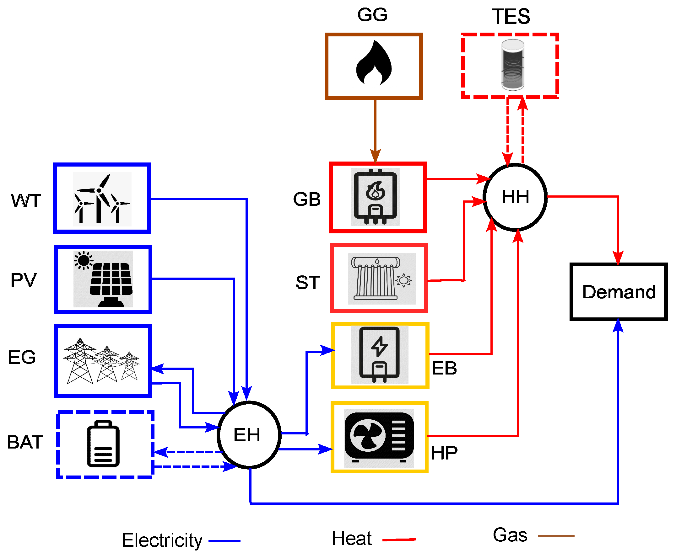
2.1. Problem Formulation
2.2. Modeling of Components
2.2.1. Photovoltaic
2.2.2. Wind Turbine
2.2.3. Gas Boiler
2.2.4. Electric Boiler
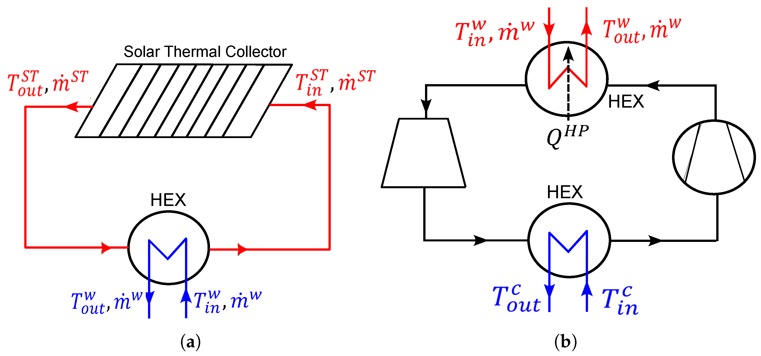
2.2.5. Solar Thermal Collector
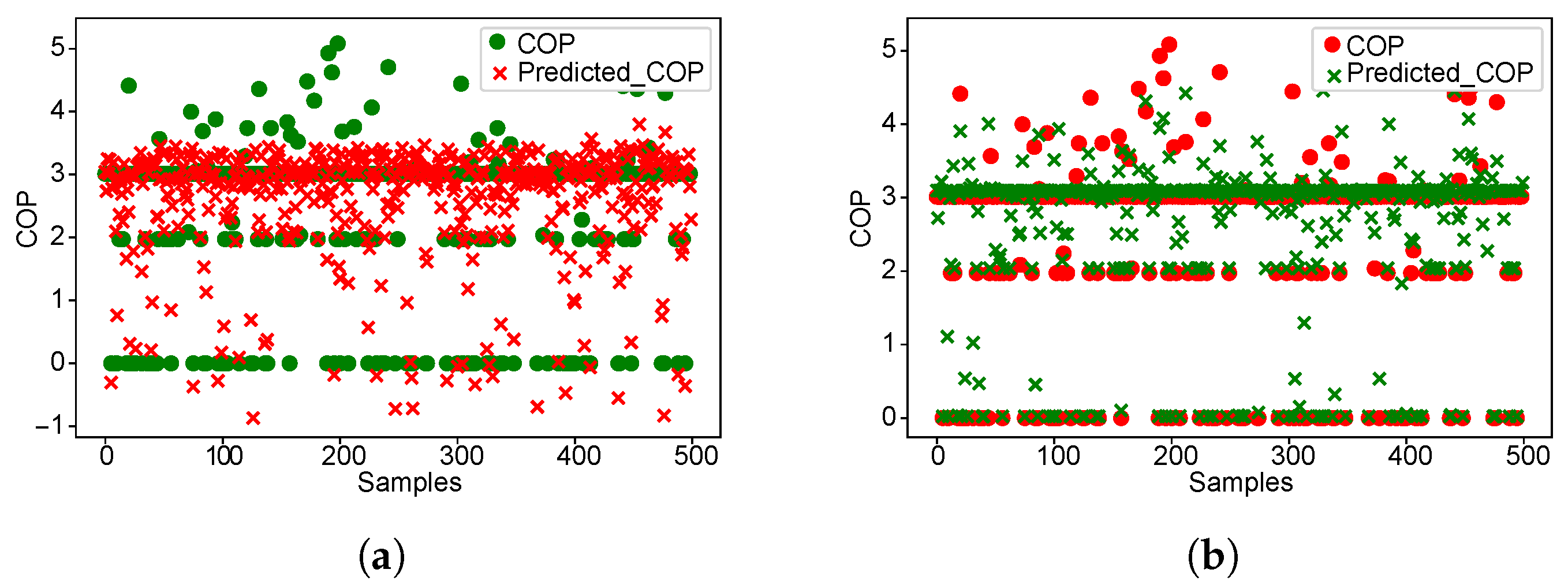
2.2.6. Heat Pump
2.2.7. Thermal Energy Storage
3. Results
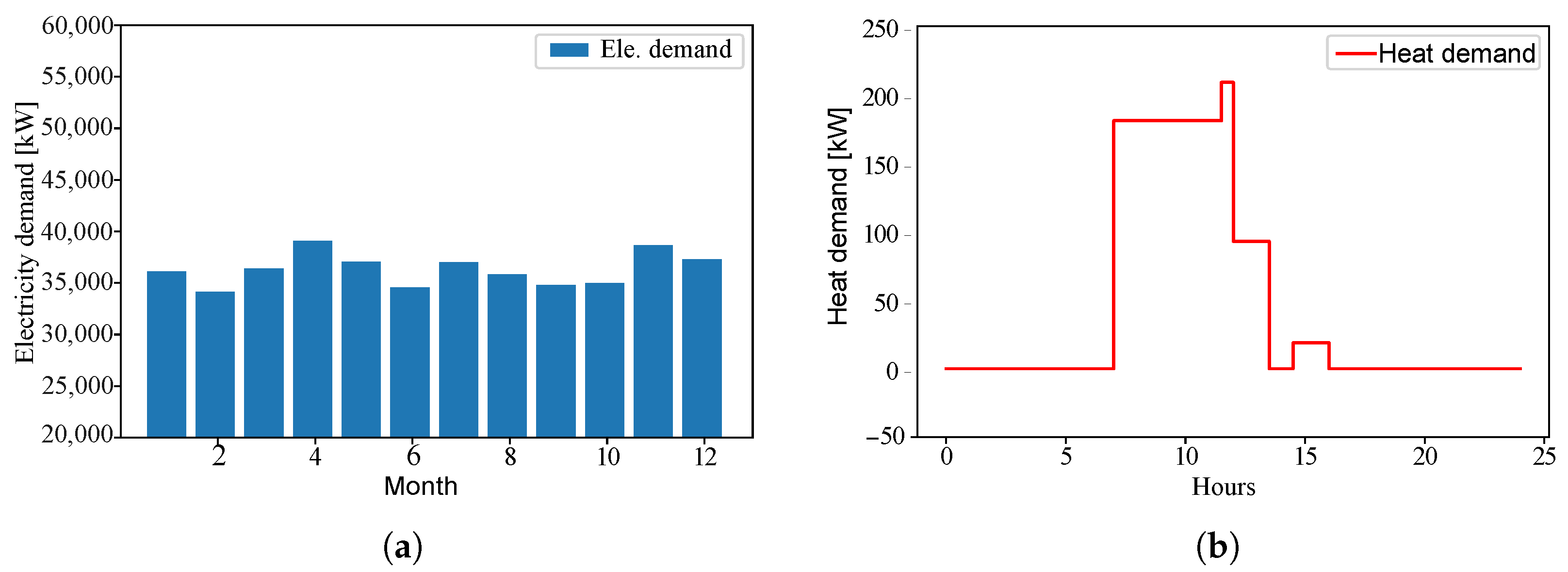
3.1. Data Analysis
3.2. Optimization Results
3.2.1. Without Tes
3.2.2. With TES
4. Conclusions and Outlook
Author Contributions
Funding
Institutional Review Board Statement
Informed Consent Statement
Data Availability Statement
Acknowledgments
Conflicts of Interest
Abbreviations
| DES | District Energy Systems |
| IES | Integrated Energy Systems |
| RES | Renewable Energy Sources |
| TES | Thermal Energy Storage |
| PV | Photovoltaic |
| WT | Wind Turbine |
| ST | Solar Thermal |
| GB | Gas Boiler |
| GG | Gas Grid |
| EG | Gas Grid |
| EB | Electric Boiler |
| EH | Electric Hub |
| HH | Heat Hub |
| HP | Heat Pump |
| MINLP | Mixed-Integer Nonlinear Programming |
| MILP | Mixed-Integer Linear Programming |
| TAC | Total Annualized Cost |
| GWI | Gloabl Warming Impact |
| OC | Operational Cost |
| CAPEX | Capital Expenditure |
| Nomenclature | |
| Letter symbols | |
| x | design variables |
| y | operational variables |
| massflow, kg/s | |
| A | area, m |
| a | annum |
| C | investment cost |
| c | specific heat capacity, kJ/kgK |
| E | energy, kWh |
| g | emission factor, g-COeq/kWh |
| global warming impact, g/kWh | |
| I | solar irradiance, kW/m |
| M | set of months |
| operational cost | |
| P | power, kW |
| p | price |
| Q | thermal capacity, kW |
| S | set of components |
| s | seconds |
| T | temperature, K |
| total annualized cost | |
| z | binary variables |
| Greek symbols | |
| maintenance cost factor | |
| interest rate | |
| numerical limit | |
| efficiency | |
| scaling exponent | |
| part load | |
| time horizon | |
| Subscripts and superscripts | |
| 0 | reference |
| ambient | |
| electric boiler | |
| electricity grid | |
| electricity | |
| gas | |
| gas boiler | |
| gas grid | |
| heat pump | |
| i | index for components |
| inlet | |
| L | loss |
| nominal | |
| outlet | |
| photovoltaic | |
| selling | |
| solar thermal | |
| u | useful |
| w | water |
| wind turbine |
References
- Voll, P.; Klaffke, C.; Hennen, M.; Bardow, A. Automated superstructure-based synthesis and optimization of distributed energy supply systems. Energy 2013, 50, 374–388. [Google Scholar] [CrossRef]
- Mayer, M.J.; Szilagyi, A.; Grof, G. Ecodesign of ground-mounted photovoltaic power plants: Economic and environmental multi-objective optimization. J. Clean. Prod. 2021, 278, 123934. [Google Scholar] [CrossRef]
- Aguilar, O.; Perry, S.J.; Kim, J.-K.; Smith, R. Design and optimization of flexible utility systems subject to variable conditions. Chem. Eng. Res. Des. 2007, 85, 1149–1168. [Google Scholar] [CrossRef]
- Velasco-Garcia, P.; Varbanov, P.S.; Arellano-Garcia, H.; Wozny, G. Utility systems operation: Optimisation based decision making. Appl. Therm. Eng. 2011, 31, 3196–3205. [Google Scholar] [CrossRef]
- Tina, G.M.; Passarello, G. Short-term scheduling of industrial co-generation systems for annual revenue maximisation. Energy 2012, 42, 46–56. [Google Scholar] [CrossRef]
- Bouvy, C.; Lucas, K. Multicriterial optimisation of communal energy supply concepts. Energy Convers. Manag. 2007, 48, 2827–2835. [Google Scholar] [CrossRef]
- Weber, C.; Shah, N. Optimisation based design of a district energy system for an eco-town in the united kingdom. Energy 2011, 36, 1292–1308. [Google Scholar] [CrossRef]
- Keirstead, J.; Shah, N. Calculating minimum energy urban layouts with mathematical programming and monte carlo analysis techniques. Comput. Environ. Urban Syst. 2011, 35, 368–377. [Google Scholar] [CrossRef]
- Lozano, M.A.; Ramos, J.C.; Carvalho, M.; Serra, L.M. Structure optimization of energy supply systems intertiary sector buildings. Energy Build. 2009, 41, 1063–1075. [Google Scholar] [CrossRef]
- Liu, P.; Pistikopoulos, E.N.; Li, Z. An energy systems engineering approach to the optimal design of energy systems in commercial buildings. Energy Policy 2010, 38, 4224–4231. [Google Scholar] [CrossRef]
- Barton, P.; Li, X. Optimal design and operation of energy systems under uncertainty. In Proceedings of the IFAC International Symposium on Dynamics and Control of Process Systems, Mumbai, India, 18–20 December 2013; Volume 46, pp. 105–110. [Google Scholar]
- Li, J.; Zhao, H. Multi-objective optimization and performance assessments of an integrated energy system based on fuel, wind and solar energies. Entropy 2021, 23, 431. [Google Scholar] [CrossRef] [PubMed]
- Patwal, R.S.; Narang, N. Multi-objective generation scheduling of integrated energy system using fuzzy based surrogate worth trade-off approach. Renew. Energy 2020, 156, 864–882. [Google Scholar] [CrossRef]
- Fazlollahi, S.; Becker, G.; Ashouri, A.; Marechal, F. Multi-objective, multi-period optimization of district energy systems: Iv–A case study. Energy 2015, 84, 365–381. [Google Scholar] [CrossRef]
- Morvaj, B.; Evins, R.; Carmeliet, J. Optimising urban energy systems: Simultaneous system sizing, operationand district heating network layout. Energy 2016, 116, 619–636. [Google Scholar] [CrossRef]
- Söderman, J.; Pettersson, F. Structural and operational optimisation of distributed energy systems. Appl. Therm. Eng. 2006, 26, 1400–1408. [Google Scholar] [CrossRef]
- Zhang, C. Data Driven Modeling and Optimization of Energy Systems. Ph.D Thesis, Nanyang Technological University, Singapore, 2019. [Google Scholar]
- Zhang, C.; Cao, L.; Romagnoli, A. On the feature engineering of building energy data mining. Sustain. Soc. 2018, 39, 508–518. [Google Scholar] [CrossRef]
- Ekonomou, L. Greek long-term energy consumption prediction using artificial neural networks. Energy 2010, 2, 512–517. [Google Scholar] [CrossRef]
- Ahmad, A.S.; Hassan, M.Y.; Abdullah, M.P.; Rahman, H.A.; Hussin, F.; Abdullah, H.; Saidur, R. A review on applications of ANN and SVM for building electrical energy consumption forecasting. Renew. Sustain. Energy Rev. 2014, 33, 102–109. [Google Scholar] [CrossRef]
- Liang, J.; Du, R. Thermal comfort control based on neural network for HVAC application. In Proceedings of the 2005 IEEE Conference on Control Applications, CCA 2005, Toronto, ON, Canada, 28–31 August 2005; pp. 819–824. [Google Scholar] [CrossRef]
- Koch, V.; Kuge, S.; Geissbauer, R.; Schrauf, S. Industry 4.0-Opportunities and Challenges of the Industrial Internet; Strategy Former Booz Company, PwC: Berlin, Germany, 2014; Volume 13, pp. 1–51. [Google Scholar]
- Caylar, P.L.; Oliver, N.; Kedar, N. Digital in Industry: From Buzzword to Value Creation; McKinsey Digit: Berlin, Germany, 2016; pp. 1–9. [Google Scholar]
- Dimopoulos, G.G.; Kougioufas, A.V.; Frangopoulos, C.A. Synthesis, design and operation optimization of a marine energy system. Energy 2008, 33, 180–188. [Google Scholar] [CrossRef]
- Sass, S.; Faulwasser, T.; Hollermann, D.E.; Kappatou, C.D.; Sauer, D.; Schutz, T.; Shu, D.Y.; Bardow, A.; Groll, L.; Hagenmeyer, V.; et al. Model compendium, data, and optimization benchmarks for sector-coupled energy systems. Comput. Chem. Eng. 2020, 135, 106760. [Google Scholar] [CrossRef]
- Umweltbundesamt Kohlendioxid-Emissionen. 2020. Available online: https://www.umweltbundesamt.de/daten/klima/treibhausgas-emissionen-in-deutschland/kohlendioxid-emissionen#herkunft-und-minderung-von-kohlendioxid-emissionen (accessed on 7 May 2023).
- Langiu, M.; Shu, D.Y.; Baader, F.J.; Hering, D.; Bau, U.; Xhonneux, A.; Müller, D.; Bardow, A.; Mitsos, A.; Dahmen, M. Comando: A next-generation open-source framework for energy systems optimization. Comput. Chem. Eng. 2021, 152, 107366. [Google Scholar] [CrossRef]
- Grahovac, M.; Liedl, P.; Frisch, J.; Tzscheutschler, P. Simplified Solar Collector Model: Hourly Simulation of Solar Boundary Condition for Multi-Energy Optimization. In Proceedings of the International Congress on Heating, Refrigerating and Air-Conditioning, Belgrade, Serbia, 1–3 December 2010; Volume 41, pp. 21–23. [Google Scholar]
- Duffie, J.; Beckman, W.A. Solar Engineering of Thermal Processes; John Wiley and Sons Inc.: Hoboken, NJ, USA, 1991. [Google Scholar]
- DIN EN 12975; Thermische Solaranlagen und Ihre Bauteile–Kollektoren–Teil 2: Prüfverfahren. DIN: Weimar, Germany, 2006.
- EU-Science-Hub Photovoltaic Geographical Information System 2020. Available online: https://joint-research-centre.ec.europa.eu/pvgis-online-tool/pvgis-tools/hourly-radiation_en (accessed on 20 January 2023).
- SPF Research. Research and Development for Sustainable Energy Systems: Flat Plate Collectors. Available online: https://www.ost.ch/ (accessed on 2 February 2023).
- Schlosser, F.; Jesper, M.; Vogelsang, J.; Walmsley, T.G.; Arpagaus, C.; Hesselbach, J. Large-scale heat pumps: Applications, performance, economic feasibility and industrial integration. Renew. Sustain. Energy Rev. 2020, 133, 110219. [Google Scholar] [CrossRef]
- Farkas, I.; Toth, J. Mathematical modelling of solar thermal collectorsand storages. Acta Technol. Agric. 2019, 22, 128–133. [Google Scholar] [CrossRef]
- Model Selection Using R-Squared (R²) Measure. Available online: https://towardsdatascience.com/the-complete-guide-to-r-squared-adjusted-r-squared-and-pseudo-r-squared-4136650fc06c (accessed on 7 March 2023).
- Ahmed, F.Y.H.; Ali, Y.H.; Shamsuddin, S.M. Using K-Fold Cross Validation Proposed Models for Spikeprop Learning Enhancements. Int. J. Eng. Technol. 2018, 7, 145–151. [Google Scholar] [CrossRef]
- Non-Convex Quadratic Optimization. Available online: https://www.gurobi.com/events/non-convex-quadratic-optimization/ (accessed on 27 February 2023).
- Mavrotas, G. Effective implementation of the e-constraint method in Multi-Objective Mathematical Programming problems. Appl. Math. Comput. 2009, 213, 455–465. [Google Scholar] [CrossRef]
- Slowik, A.; Kwasnicka, H. Evolutionary algorithms and their applications to engineering problems. Neural Comput. Appl. 2020, 2, 12363–12379. [Google Scholar] [CrossRef]


| Name | Parameter | Value |
|---|---|---|
| electricity buying price | 0.31 [€] | |
| electricity selling price | 0.06 [€] | |
| gas buying price | 0.15 [€] | |
| CO factor for net consumed electricity | 0.349 [kg-COeq/kWh] | |
| CO factor for consumed gas | 0.244 [kg-COeq/kWh] |
| Components | Reference Capacity | [€] | |||||
|---|---|---|---|---|---|---|---|
| PV | [m] | 1400 | 0.95 | 0.01 | 0.03 | 10 | 0 |
| WT | [kW] | 5000 | 0.95 | 0.03 | 0.03 | 10 | 0.33 |
| ST | [m] | 400 | 0.95 | 0.02 | 0.03 | 10 | 0 |
| GB | [kW] | 2700 | 0.45 | 0.02 | 0.03 | 10 | 0.2 |
| EB | [kW] | 70 | 0.95 | 0.01 | 0.03 | 10 | 0 |
| HP | [kW] | 1655 | 0.66 | 0.02 | 0.03 | 10 | 0 |
| TES | [kWh] | 200 | 0.86 | 0.01 | 0.03 | 10 | 0 |
| Components | Design Variables x | Operational Variables y | Constant Parameters c | Input Parameters in Each Time-Step | Total Number of Variables |
|---|---|---|---|---|---|
| PV | , | I | 3 | ||
| WT | , | - | v | 4 | |
| GB | , | - | 4 | ||
| EB | , | - | 4 | ||
| ST | , , | I, , | 5 | ||
| HP | a, b, c, d, , | 6 | |||
| TES | , | - | 4 | ||
| Electric grid | - | - | - | 2 | |
| Gas grid | - | - | - | 1 |
| Collector | [W/(mK)] | [W/(mK)] | ||
|---|---|---|---|---|
| Flat plate | 0.79 | 4.03 | 0.0078 | 0.86 |
| ST | HP | Total Number of Variables | Total Number of Constraints |
|---|---|---|---|
| Physics-driven | Physics-driven | 1741 | 2748 |
| Data-driven | Data-driven | 1353 | 2244 |
| Data-driven | Physics-driven | 1525 | 2316 |
| Physics-driven | Data-driven | 1669 | 2676 |
| Component | Inputs | Output | Number of Data Samples |
|---|---|---|---|
| ST | , , I, A | 439,199 | |
| HP | , , , | 206,054 |
| Model | Specification | Training Time for ST [s] | Training Time for HP [s] | for ST | for HP |
|---|---|---|---|---|---|
| LR | degree 1 | 2.12 | 1.82 | 0.96 | 0.45 |
| PR-1 | degree 2 | 5.33 | 4.31 | 0.972 | 0.68 |
| PR-2 | degree 3 | 11.26 | 9.25 | 0.986 | 0.825 |
| ANN-1 | 2 hidden layers 5 neurons each | 1254 | 1008 | 0.999 | 0.862 |
| ANN-2 | 3 hidden layers 7 neurons each | 1852 | 1369 | 0.845 | 0.982 |
| ST | HP | Total Number of Variables | Total Number of Constraints | Computational Time [s] | Accuracy [%] |
|---|---|---|---|---|---|
| Physics-driven | Physics-driven | 2175 | 3325 | 18,025 | 100 |
| PR-2 | Physics-driven | 1959 | 2893 | 12,671 | 90.3 |
Disclaimer/Publisher’s Note: The statements, opinions and data contained in all publications are solely those of the individual author(s) and contributor(s) and not of MDPI and/or the editor(s). MDPI and/or the editor(s) disclaim responsibility for any injury to people or property resulting from any ideas, methods, instructions or products referred to in the content. |
© 2024 by the authors. Licensee MDPI, Basel, Switzerland. This article is an open access article distributed under the terms and conditions of the Creative Commons Attribution (CC BY) license (https://creativecommons.org/licenses/by/4.0/).
Share and Cite
Kansara, R.; Lockan, M.; Roldán Serrano, M.I. Combined Physics- and Data-Driven Modeling for the Design and Operation Optimization of an Energy Concept Including a Storage System. Energies 2024, 17, 350. https://doi.org/10.3390/en17020350
Kansara R, Lockan M, Roldán Serrano MI. Combined Physics- and Data-Driven Modeling for the Design and Operation Optimization of an Energy Concept Including a Storage System. Energies. 2024; 17(2):350. https://doi.org/10.3390/en17020350
Chicago/Turabian StyleKansara, Rushit, Michael Lockan, and María Isabel Roldán Serrano. 2024. "Combined Physics- and Data-Driven Modeling for the Design and Operation Optimization of an Energy Concept Including a Storage System" Energies 17, no. 2: 350. https://doi.org/10.3390/en17020350
APA StyleKansara, R., Lockan, M., & Roldán Serrano, M. I. (2024). Combined Physics- and Data-Driven Modeling for the Design and Operation Optimization of an Energy Concept Including a Storage System. Energies, 17(2), 350. https://doi.org/10.3390/en17020350